Complexity of colouring problems restricted to unichord-free and $\{$square,unichord$\}$-free graphst1

Abstract

A unichord in a graph is an edge that is the unique chord of a cycle. A square is an induced cycle on four vertices. A graph is unichord-free if none of its edges is a unichord. We give a slight restatement of a known structure theorem for unichord-free graphs and use it to show that, with the only exception of the complete graph $K_{4}$, every square-free, unichord-free graph of maximum degree 3 can be total-coloured with four colours. Our proof can be turned into a polynomial time algorithm that actually outputs the colouring. This settles the class of square-free, unichord-free graphs as a class for which edge-colouring is NP-complete but total-colouring is polynomial.

pfProof

[t1]February 3, 2012. An extended abstract of this paper was presented at ISCO 2010, the International Symposium on Combinatorial Optimization, and appeared in Electronic Notes in Discrete Mathematics 36 (2010) 671–678.

1 Introduction

In the present paper, we deal with simple connected graphs. A graph $G$ has vertex set $V(G)$ and edge set $E(G)$. An element of $G$ is one of its vertices or edges and the set of elements of $G$ is denoted by $S(G):=V(G)\cup E(G)$. Two vertices $u,v\in V(G)$ are adjacent if $uv\in E(G)$; two edges $e_{1},e_{2}\in E(G)$ are adjacent if they share a common endvertex; a vertex $u$ and an edge $e$ are incident if $u$ is an endvertex of $e$. For a graph $G=(V,E)$ and $V^{\prime}\subseteq V$, $G[V^{\prime}]$ denotes the subgraph of $G$ induced by $V^{\prime}$. The degree of a vertex $v$ in $G$ is the number of edges of $G$ incident to $v$. We use the standard notation of $K_{n}$, $K_{m,n}$ and $C_{n}$ for complete graphs, complete bipartite graphs and cycle-graphs, respectively.

An edge-colouring is an association of colours to the edges of a graph in such a way that no adjacent edges receive the same colour. The chromatic index of a graph $G$, denoted $\chi^{\prime}(G)$, is the least number of colours sufficient to edge-colour this graph. Clearly, $\chi^{\prime}(G)\geq\Delta(G)$, where $\Delta(G)$ denotes the maximum degree of a vertex in $G$. Vizing’s theorem Vizing states that every graph $G$ can be edge-coloured with $\Delta(G)+1$ colours. By Vizing’s theorem only two values are possible for the chromatic index of a graph: $\chi^{\prime}(G)=\Delta(G)$ or $\Delta(G)+1$. If a graph $G$ has chromatic index $\Delta(G)$, then $G$ is said to be Class 1; if $G$ has chromatic index $\Delta(G)+1$, then $G$ is said to be Class 2.

A total-colouring is an association of colours to the elements of a graph in such a way that no adjacent or incident elements receive the same colour. The total chromatic number of a graph $G$, denoted $\chi_{T}(G)$, is the least number of colours sufficient to total-colour this graph. Clearly, $\chi_{T}(G)\geq\Delta(G)+1$. The Total Colouring Conjecture (TCC) states that every graph $G$ can be total-coloured with $\Delta(G)+2$ colours. By the TCC only two values would be possible for the total chromatic number of a graph: $\chi_{T}(G)=\Delta(G)+1$ or $\Delta(G)+2$. If a graph $G$ has total chromatic number $\Delta(G)+1$, then $G$ is said to be Type 1; if $G$ has total chromatic number $\Delta(G)+2$, then $G$ is said to be Type 2. The TCC has been verified in restricted cases, such as graphs with maximum degree $\Delta\leq 5$ Kostochka1 ; Kostochka2 ; Rosenfeld ; Vijayaditya , but the general problem is open since 1964, exposing how challenging the problem of total-colouring is.

It is NP-complete to determine whether the total chromatic number of a graph $G$ is $\Delta(G)+1$ SanchezArroyo1 ; SanchezArroyo . Remark that the original NP-completeness proof was a reduction from the edge-colouring problem, suggesting that, for most graph classes, total-colouring would be harder than edge-colouring. The present paper presents the first example of an unexpected graph class for which edge-colouring is NP-complete while total-colouring is polynomial. For a discussion on the search of complexity separating classes for edge-colouring and total-colouring please refer to BipJBCS .

A square is an induced cycle on four vertices. A unichord is an edge that is the unique chord of a cycle in the graph. In the present work, we consider total-colouring restricted to $\{$square,unichord$\}$-free graphs — that is, graphs that do not contain (as an induced subgraph) a cycle with a unique chord nor a square. The class of unichord-free graphs was studied by Trotignon and Vušković tv . They give a structure theorem for the class, and use it to develop algorithms for recognition and vertex-colouring. Basically, this structure result states that every unichord-free graph can be built starting from a restricted set of basic graphs and applying a series of known “gluing” operations. The following results are obtained in tv for unichord-free graphs: an $O(nm)$ recognition algorithm, an $O(nm)$ algorithm for optimal vertex-colouring, an $O(n+m)$ algorithm for maximum clique, and the NP-completeness of the maximum stable set problem.

Machado, Figueiredo and Vušković Edge-tv investigated whether the structure results of tv could be applied to obtain a polynomial-time algorithm for the edge-colouring problem restricted to unichord-free graphs. The authors obtained a negative answer by establishing the NP-completeness of the edge-colouring problem restricted to unichord-free graphs. The authors investigated also the complexity of the edge-colouring in the subclass of $\{$square,unichord$\}$-free graphs. The class of $\{$square,unichord$\}$-free graphs can be viewed as the class of graphs that can be constructed from the same set of basic graphs, but using one less operation (the so-called 1-join operation is forbidden). For $\{$square,unichord$\}$-free graphs, an interesting dichotomy is proved in Edge-tv : if the maximum degree is not 3, the edge-colouring problem is polynomial, while for inputs with maximum degree 3, the problem is NP-complete.

It is a natural step to investigate the complexity of total-colouring restricted to classes for which the complexity of edge-colouring is already established. This approach is observed, for example, in the classes of outerplanar graphs Zhang , series-parallel graphs WangPang , and some subclasses of planar graphs WeifanWang and join graphs OneKindJoin ; OutroJoin . One important motivation for this approach is the search for “separating” classes, that are classes for which the complexities of edge-colouring and total-colouring differ. We must mention that all previously known separating classes, in this sense, are classes for which edge-colouring is polynomial and total-colouring is NP-complete, such as the case of bipartite graphs. In other words, there is no known example of a class for which edge-colouring is NP-complete and total-colouring is polynomial, an evidence that total-colouring might be “harder” than edge-colouring.

Considering the recent interest in colouring problems restricted to unichord-free and $\{$square,unichord$\}$-free graphs, specially the results Total-tv on total-colouring $\{$square,unichord$\}$-free graphs of maximum degree at least 4, it is natural to investigate the remaining case of total-colouring restricted to $\{$square,unichord$\}$-free graphs of maximum degree 3. In the present work, we prove that, except for the complete graph $K_{4}$, every $\{$square,unichord$\}$-free graph of maximum degree 3 is Type 1. Our proof can easily be turned into a polynomial time algorithm that outputs the colouring whose existence is proved (we omit the details of the implementation). Table 1 summarizes the current status of colouring problems restricted to unichord-free and $\{$square,unichord$\}$-free graphs.

Problem $\setminus$ Class	unichord-free	$\{$sq.,un.$\}$-free, $\Delta\geq 4$	$\{$sq.,un.$\}$-free, $\Delta=3$
vertex-colouring	Polynomial tv	Polynomial tv	Polynomial tv
edge-colouring	NP-complete Edge-tv	Polynomial Edge-tv	NP-complete Edge-tv
total-colouring	NP-complete Total-tv	Polynomial Total-tv	Polynomial∗

Table 1: Computational complexity of colouring problems restricted to unichord-free and to $\{$square,unichord$\}$-free graphs — star indicates result established in the present paper.

Observe in Table 1 the interesting degree dichotomy with respect to edge-colouring $\{$square,unichord$\}$-free graphs. Since the technique used in Total-tv to total-colour $\{$square,unichord$\}$-free graphs could only be applied to the case of maximum degree at least 4, a similar dichotomy could be expected for the total-colouring problem. Surprisingly, we establish in the present work that such dichotomy does not exist. It is additionally interesting to note that different approaches were needed to solve the total-colouring problem in the cases $\Delta\geq 4$ and $\Delta=3$. Note that a natural subclass of unichord-free graphs is the class of chordless graphs, that are the graphs where all cycles are chordless. For these graphs, we have proved that edge- and total-colouring are all polynomially solvable, with no restriction on the degree and the presence of squares Chordless .

In Section 2, we recall the structure theorem for unichord-free graphs. We restate it in a slightly different form that is well-fit to our goal of total-colouring. In Section 3, we prove the main result of the paper that non-complete $\{$square, unichord$\}$-free graphs with maximum degree 3 are Type 1.

2 Decomposing unichord-free graphs

We revisit the decomposition result for unichord-free tv graphs, stating it in a new form that will be suitable for total-colouring.

2.1 Decomposition theorem

The Petersen graph is the cubic graph on vertices $\{a_{1},\dots,a_{5},b_{1},\dots,b_{5}\}$ so that both $a_{1}a_{2}a_{3}a_{4}a_{5}a_{1}$ and $b_{1}b_{2}b_{3}b_{4}b_{5}b_{1}$ are chordless cycles, and such that the only edges between some $a_{i}$ and some $b_{i}$ are $a_{1}b_{1}$, $a_{2}b_{4}$, $a_{3}b_{2}$, $a_{4}b_{5}$, $a_{5}b_{3}$. Figure 1(a) exhibits a (total-coloured) graph isomorphic to the Petersen graph. We denote by $P$ the Petersen graph and by $P^{*}$ the graph obtained from $P$ by the removal of one vertex. Observe that $P$ is unichord-free.

The Heawood graph is the cubic bipartite graph on vertices $\{a_{1},\dots,a_{14}\}$ so that $a_{1}a_{2}\dots a_{14}a_{1}$ is a cycle, and such that the only other edges are $a_{1}a_{10}$, $a_{2}a_{7}$, $a_{3}a_{12}$, $a_{4}a_{9}$, $a_{5}a_{14}$, $a_{6}a_{11}$, $a_{8}a_{13}$. Figure 1(b) exhibits a (total-coloured) graph isomorphic to the Heawood graph. The Hamiltonian cycle from the definition is shown in bold edges. We denote by $H$ the Heawood graph and by $H^{*}$ the graph obtained from $H$ by the removal of one vertex. Observe that $H$ is unichord-free.

It essential for understanding what follows to notice that the Petersen and Heawood graphs are both vertex-transitive. It is also helpful to know their most classical embeddings, as shown for instance in tv .

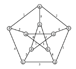
(a) Petersen graph.

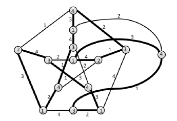
(b) Heawood graph.

Figure 1: 4-total-colourings of the Petersen graph and of the Heawood graph.

A graph is strongly 2-bipartite if it is square-free and bipartite with bipartition $(X,Y)$ where every vertex in $X$ has degree 2 and every vertex in $Y$ has degree at least 3. A strongly 2-bipartite graph is unichord-free because any chord of a cycle is an edge between two vertices of degree at least three, so every cycle in a strongly 2-bipartite graph is chordless.

A cutset $S$ of a connected graph $G$ is a set of vertices or a set of edges whose removal disconnects $G$. A decomposition of a graph is the systematic removal of cutsets to obtain smaller graphs (by adding vertices and edges to connected components of $G\setminus S$), called the blocks of decomposition, repeating this until a set of basic (undecomposable) graphs is obtained. The goal of decomposing a graph is trying to solve a problem on the original graph by combining the solutions on the blocks. The following cutsets are used in the decomposition theorem of Trotignon and Vušković for unichord-free graphs tv :

• A 1-cutset of a connected graph $G=(V,E)$ is a vertex $v$ such that $V$ can be partitioned into sets $X$, $Y$ and $\{v\}$, so that there is no edge between $X$ and $Y$. We say that $(X,Y,v)$ is a split of this 1-cutset.

• A special 2-cutset of a connected graph $G=(V,E)$ is a pair of non-adjacent vertices $a,b$, both of degree at least three, such that $V$ can be partitioned into sets $X$, $Y$ and $\{a,b\}$ so that: $|X|\geq 2$, $|Y|\geq 2$; there is no edge between $X$ and $Y$, and both $G[X\cup\{a,b\}]$ and $G[Y\cup\{a,b\}]$ contain an $ab$-path. We say that $(X,Y,a,b)$ is a split of this special 2-cutset. Note that in tv , special 2-cutsets are called proper 2-cutsets. We apologize for changing the terminology, but we find it more convenient to keep the “proper 2-cutset” for the restatement given in Section 2.2.

• A proper 1-join of a graph $G=(V,E)$ is a partition of $V$ into sets $X$ and $Y$ such that there exist sets $A\subseteq X$ and $B\subseteq Y$ so that: $|A|\geq 2$, $|B|\geq 2$; $A$ and $B$ are stable sets; there are all possible edges between $A$ and $B$; there is no other edge between $X$ and $Y$. We say that $(X,Y,A,B)$ is a split of this proper 1-join.

We are now ready to state a decomposition result for unichord-free graphs.

Theorem 1.

(Trotignon and  Vušković tv ) If $G$ is a connected unichord-free graph, then either $G$ is a complete graph, or a cycle, or a strongly 2-bipartite graph, or an induced subgraph of the Petersen graph, or an induced subgraph of the Heawood graph, or $G$ has a 1-cutset, a special 2-cutset, or a proper 1-join.

The decomposition blocks with respect to 1-cutsets and special 2-cutsets are defined below (we do not use here the blocks with respect to proper 1-joins).

The block $G_{X}$ (resp. $G_{Y}$) of a graph $G$ with respect to a 1-cutset with split $(X,Y,v)$ is $G[X\cup\{v\}]$ (resp. $G[Y\cup\{v\}]$).

The blocks $G_{X}$ and $G_{Y}$ of a graph $G$ with respect to a special 2-cutset with split $(X,Y,a,b)$ are defined as follows. If there exists a vertex $c$ of $G$ such that $N_{G}(c)=\{a,b\}$, then let $G_{X}=G[X\cup\{a,b,c\}]$ and $G_{Y}=G[Y\cup\{a,b,c\}]$. Otherwise, block $G_{X}$ (resp. $G_{Y}$) is the graph obtained by taking $G[X\cup\{a,b\}]$ (resp. $G[Y\cup\{a,b\}]$) and adding a new vertex $c$ adjacent to $a,b$. Vertex $c$ is called the marker of the block $G_{X}$ (resp. $G_{Y}$).

The decomposition blocks of a unichord-free graph with respect to 1-cutsets and special 2-cutsets are constructed in such a way that they remain unichord-free tv . Additionally, the decomposition blocks of a $\{$square,unichord$\}$-free graph are themselves $\{$square,unichord$\}$-free Edge-tv .

2.2 Restated decomposition theorem

We derive a restatement of the decomposition result for unichord-free graphs that fits better to our total-colouring purposes (possibly for other purposes as well). The proposed restatement needs the following notion of proper 2-cutset.

A proper 2-cutset of a graph $G=(V,E)$ is a pair of non-adjacent vertices $a,b$ such that $V$ can be partitioned into sets $X$, $Y$ and $\{a,b\}$ so that: $|X|\geq 2$, $|Y|\geq 2$; there is no edge between $X$ and $Y$; and both $G[X\cup\{a,b\}]$ and $G[Y\cup\{a,b\}]$ contain an $ab$-path but none of them is an $ab$-path. We say that $(X,Y,a,b)$ is a split of this proper 2-cutset. Note that a proper 2-cutset is a particular kind of special 2-cutset (so we may still use the notion of block of decomposition as defined previously).

A branch vertex of a graph is any vertex of degree at least 3, and we call branch any path whose endvertices are branch vertices and whose internal vertices are not. Observe that a 2-connected graph that is not a cycle can be edge-wise partitioned into its branches. A graph is sparse if its branch vertices form a stable set (so every edge is incident to at least one vertex of degree at most 2). Note that every strongly 2-bipartite graph is sparse. The reduced graph of a 2-connected graph $G$ that is not a cycle is the graph obtained from $G$ by contracting every branch of length at least 3 into a branch of length 2.

A 2-extension of a graph $G$ is any graph obtained by (first) deleting vertices from $G$ and (second) subdividing edges incident to at least one vertex of degree 2. Note that the unichord-free class is closed under taking 2-extensions.

We can now restate the decomposition theorem of Trotignon and Vušković for unichord-free graphs. The difference with the original theorem is that we use the more precise “proper” 2-cutset instead of the “special” 2-cutset. The price to pay for that is an extension of the basic classes: instead of the strongly 2-bipartite graphs, induced subgraphs of Petersen and induced subgraphs of Heawood, we have to use the less precise sparse graphs, 2-extensions of Petersen and 2-extensions of Heawood respectively. Another small difference is that cycles do not form a separate basic class anymore since they are sparse.

Theorem 2.

If $G$ is a connected unichord-free graph, then either $G$ is a complete graph, or a sparse graph, or a 2-extension of Petersen or Heawood graph, or $G$ has a 1-cutset, a proper 2-cutset, or a proper 1-join.

Proof: We may assume that $G$ is not a cycle and is 2-connected (for otherwise, it is sparse or has a 1-cutset). Let $G^{\prime}$ be the reduced graph of $G$. Observe that $G$ can be obtained from $G^{\prime}$ by subdividing edges incident to at least one vertex of degree 2, that $G^{\prime}$ is not a cycle, and that $G^{\prime}$ is 2-connected. Also, $G^{\prime}$ is unichord-free, since contracting a path of length at least 3 into a path of length 2 does not create nor destroy chords of cycles.

We apply the decomposition Theorem 1 to $G^{\prime}$. If $G^{\prime}$ is a complete graph on at least 4 vertices, then in fact $G=G^{\prime}$, so we are done. If $G^{\prime}$ is a strongly 2-bipartite graph then $G$ is sparse. If $G^{\prime}$ is an induced subgraph of the Petersen graph or of the Heawood graph, then $G$ is a 2-extension of Petersen or Heawood graph. If $G^{\prime}$ has a special 2-cutset $\{a,b\}$ with split $(X,Y,a,b)$, then $\{a,b\}$ is a proper 2-cutset of $G$ (since $G^{\prime}$ is reduced, no side $G[X\cup\{a,b\}]$ or $G[Y\cup\{a,b\}]$ of a special 2-cutset in $G^{\prime}$ can be a path, because this would imply that $|X|=1$ or $|Y|=1$).

Finally consider the case where $G^{\prime}$ has a proper 1-join with split $(X,Y,A,B)$. Suppose that $(X,Y,A,B)$ is chosen so that the number $k$ of vertices of degree 2 in $A\cup B$ is minimal. If $k=0$, then all vertices in $A\cup B$ have degree at least 3, so $G$ is obtained from $G^{\prime}$ by subdividing edges with both ends in $X$ or both ends in $Y$, so that the edges between $A$ and $B$ still form a proper 1-join in $G$. Hence, we may assume that in $G^{\prime}$, there is a vertex $u\in A$ (up to symmetry) of degree 2. It follows that $|B|=2$, say $B=\{v,w\}$ and $B$ is the neighborhood of $u$ in $G^{\prime}$. If $A\geq 3$, then $(X\setminus\{u\},Y\cup\{u\},A\setminus\{u\},B)$ is a split of a proper 1-join of $G^{\prime}$ that contradicts the minimality of $k$. So, $|A|=2$, say $A=\{u,u^{\prime}\}$. Since $G$ is 2-connected, $u^{\prime}$ cannot be a 1-cutset, so in fact $X=A=\{u,u^{\prime}\}$. If $|Y|\geq 4$, then $(X,Y\setminus\{v,w\},v,w)$ is a split of a special 2-cuset of $G^{\prime}$, so we are done as in the previous paragraph. Hence, $|Y|\leq 3$. Now, all vertices in $G^{\prime}$ have degree at most 2, except possibly $v$ and $w$ that are non-adjacent. It follows that $G^{\prime}$ is sparse, and so is $G$ (in fact, $4\leq|V(G^{\prime})|\leq 5$, and $G^{\prime}$ is isomorphic to the square or to $K_{2,3}$).  

A more precise theorem is obtained for 2-connected square-free graphs.

Theorem 3.

If $G$ is a 2-connected {square, unichord}-free graph, then either $G$ is a complete graph, or a sparse graph, or a 2-extension of Petersen or Heawood graph, or has a proper 2-cutset.

Proof: Follows directly from Theorem 2 because a 1-join cannot occur in a square-free graph (if a graph has a 1-join, it must contain a square, formed by any two vertices from $A$ and two vertices from $B$).  

The following lemma restates the extremal decomposition of tv .

Lemma 4.

Let $G$ be a 2-connected $\{$square,unichord$\}$-free graph and let $(X,Y,a,b)$ be a split of a proper 2-cutset of $G$ such that $|X|$ is minimum among all possible such splits. Then $a$ and $b$ both have at least two neighbors in $X$, and $G_{X}$ is a sparse graph or is a 2-extension of Petersen or Heawood graph.

Proof: First, we show that $a$ and $b$ both have at least two neighbors in $X$. Suppose that one of $a,b$, say $a$, has a unique neighbor $a^{\prime}\in X$. We claim that $a^{\prime}$ is not adjacent to $b$. For otherwise, since $G[X\cup\{a,b\}]$ does not induce a path and $G$ is 2-connected, there is a path in $X$ from $b$ to $a^{\prime}$, that together with a path from $a$ to $b$ with interior in $Y$ form a cycle with a unique chord: $a^{\prime}b$. So, $a^{\prime}$ is not adjacent to $b$. Hence, by replacing $a$ by $a^{\prime}$, we obtain a proper 2-cutset that contradicts the minimality of $X$.

Denote by $m$ the marker of $G_{X}$. One can easily check that the block $G_{X}$ is a 2-connected unichord-free graph. Also, $G_{X}$ is square-free. Indeed, since $G$ is square-free, a square in $G_{X}$ must be formed by $m,a,b$ and a vertex $x\in X$ adjacent to $a$ and $b$. If $x$ has degree 2, there is a contradiction, because from the definition of a block of decomposition, $x$ should have been used as the marker vertex. So, $x$ has a neighbor $x^{\prime}\in X$. Since $G_{X}$ is 2-connected, in $G_{X}\setminus x$, there is a path $P=x^{\prime}\dots y$ such that $y$ has a neighbor in $\{a,b\}$. We choose such a path of minimum length. Since $G$ is square-free, $y$ has in fact a unique neighbor in $\{a,b\}$. Hence, $V(P)\cup\{a,b,x,m\}$ is a cycle with a unique chord in $G_{X}$, a contradiction.

Suppose $G_{X}$ has a proper 2-cutset with split $(X_{1},X_{2},u,v)$. Choose it so that $u$ and $v$ both have degree at least 3 (this is possible as explained at the beginning of the proof). Note that $m\notin\{u,v\}$. Observe that, if $\{a,b\}=\{u,v\}$, then $(X_{1},Y\cup X_{2},a,b)$ would be a split of a proper 2-cutset of $G$, contradicting the minimality of $|X|$. So $\{a,b\}\neq\{u,v\}$. Assume w.l.o.g. $b\not\in\{u,v\}$.

Suppose $a\not\in\{u,v\}$. Then w.l.o.g. $\{a,b\}\subseteq X_{1}$, and hence $(X_{1}\cup Y,X_{2},u,v)$ — with $m$ removed if $m$ is not an original vertex of $G$ — is a split of a proper 2-cutset of $G$, contradicting the minimality of $|X|$. Therefore $a\in\{u,v\}$. Then w.l.o.g. $m\in X_{1}$, and hence $(X_{1}\cup Y,X_{2},u,v)$ — with $m$ removed if $m$ is not an original vertex of $G$ — is a proper 2-cutset of $G$ whose block of decomposition $G_{X_{2}}$ is smaller than $G_{X}$, contradicting the minimality of $|X|$.

In any case, we reach a contradiction which means that $G_{X}$ has no proper 2-cutset. Since $a$ and $b$ are not adjacent, $G_{X}$ is not a complete graph. Hence, by Theorem 3, $G_{X}$ must be sparse or a 2-extension of Petersen or Heawood graph.  

3 Total-colouring $\{$square,unichord$\}$-free graphs with maximum degree 3

In the present section, we prove that the only Type 2 $\{$square,unichord$\}$-free graph of maximum degree 3 is $K_{4}$.

Theorem 5.

Every $\{$square,unichord$\}$-free graph with maximum degree at most 3 different from $K_{4}$ is 4-total-colourable.

For the proof of Theorem 5, we need three lemmas — Lemmas 6, 7 and 8 — that give sufficient conditions to extend a partial 4-total-colouring of a graph to a 4-total-colouring of this graph. Lemmas 6 and 7 are proved in Chordless ; for the sake of completeness, all proofs are included here.

Lemma 6.

Let $k\geq 3$ be an integer, and let $P=p_{1}\dots p_{k}$ be a path. Suppose that $p_{1},p_{1}p_{2},p_{k-1}p_{k},p_{k}$ are coloured with 2 or 3 colours, respectively $c_{1}$, $c_{2}$, $c_{2k-2}$ and $c_{2k-1}$, such that adjacent elements receive different colours and we do not have

$$c_{1}=c_{2k-2}\text{ and }c_{2}=c_{2k-1}.$$

This can be extended to a 4-total-colouring of $P$.

Proof: We view a total-colouring of $P$ as a sequence $c_{1},\dots,c_{2k-1}$ of integers from $\{1,2,3,4\}$, that are the colours of the elements of $P$ as they appear when walking along $P$ from $p_{1}$ to $p_{k}$. The sequence is proper when any two numbers at distance at most 2 along the sequence have different values (this corresponds exactly to a total-colouring of the path). What we need to prove is that when $c_{1},c_{2},c_{2k-2},c_{2k-1}$ receive values among $1,2,3$, and these values are different for distinct elements at distance at most 2, and we do not have $c_{1}=c_{2k-2}\text{ and }c_{2}=c_{2k-1}$, then this can be extended to a proper sequence $c_{1},\dots,c_{2k-1}$.

We proceed by induction on $k$. If $k=3$ then only $c_{3}$ has no value, and the fourth number 4 is available for it. So suppose $k\geq 4$. Among colours 1, 2, 3, at least one, say 3, is used at most once for $c_{1},c_{2},c_{2k-2},c_{2k-1}$. Up to symmetry we may assume that colour 3 is not used for $c_{1},c_{2}$. We put $c_{3}=3$. Now we consider two cases.

If $\{c_{2},c_{2k-2}\}=\{1,2\}$, say $c_{2}=2,c_{2k-2}=1$, then we must have $c_{1}=1$ because 3 is not used for $c_{1}$, so $c_{2k-1}=3$ because otherwise we have $c_{2k-1}=2$ implying $c_{1}=c_{2k-2}\text{ and }c_{2}=c_{2k-1}$ which is forbidden by assumption. So, we put $c_{2k-3}=2$. By the induction hypothesis, we complete the sequence $c_{2},\dots,c_{2k-2}$.

If $\{c_{2},c_{2k-2}\}\neq\{1,2\}$, then we put $c_{2k-3}=4$. We claim that $|\{c_{2},c_{3},c_{2k-3},c_{2k-2}\}|\leq 3$. Indeed, since $\{c_{2},c_{2k-2}\}\neq\{1,2\}$, either $c_{2}=c_{2k-2}$ (which proves the claim), or $c_{2k-2}=3$ (which also proves the claim because $c_{3}=3$). Also, $c_{2}\neq c_{2k-3}=4$. Hence, by the induction hypothesis, we complete the sequence $c_{2},\dots,c_{2k-2}$.  

Lemma 7.

Let $G$ be a 2-connected sparse graph of maximum degree 3. Graph $G$ is 4-total-colourable. Moreover suppose that $u$ is a vertex of degree 2 that has two neighbors $a,b$ of degree 3 and suppose that $a$, $b$, $au$, $ub$ receive respectively colours 1, 1, 2, 3. This can be extended to a total-colouring of $G$ using $4$ colours.

Proof: Note that, because of its maximum degree, $G$ is not a cycle. Let $G^{\prime}$ be the reduced graph of $G$. We first total-colour several elements of $G^{\prime}$. We give to all branch vertices of $G^{\prime}$ colour 1. We edge-colour $G^{\prime}$ with colours $2,3,4$ (up to a relabeling, it is possible to give colour $2,3$ to $au$, $ub$ respectively). This is possible, because $G^{\prime}$ is bipartite and a classical theorem due to König says that any bipartite graph $H$ is $\Delta(H)$-edge colourable. We extend this to a total-colouring of $G$ by considering one by one the branches of $G$ (that edge-wise partition $G$ and vertex-wise cover $G$). Let $P=p_{1}\dots p_{k}$, ($k\geq 3$ since $G$ is sparse) be such a branch. The following elements are precoloured: $p_{1},p_{1}p_{2},p_{k-1}p_{k},p_{k}$. The precolouring satisfies the requirement of Lemma 6, so we can extend it to $P$.  

Lemma 8.

Let $G$ be a 2-connected 2-extension of Petersen or Heawood graph. Then $G$ is 4-total-colourable. Moreover suppose that $u$ is a vertex of degree 2 that has two neighbors $a,b$ of degree 3 and suppose that $a$, $b$, $au$, $ub$ receive respectively colours 1, 1, 2, 3. This can be extended to a total-colouring of $G$ using $4$ colours.

Proof: If $G$ is the Petersen or the Heawood graph, the total-colouring is shown on Fig. 1(a).

Suppose first that $G$ is obtained from the Petersen graph by deleting exactly one vertex (and then subdividing edges incident to at least one degree-2 vertex). This means that the reduced graph of $G$ is $P^{*}$. On Figure 2, a 4-total-colouring of $P^{*}$ is shown. Note that, for all paths of length 2 of $P^{*}$, say $xyz$, the colors of $x,xy,yz,z$ never have the pattern $ABAB$. This means that Lemma 6 allows to extend this 4-total-colouring of $P^{*}$ to a 4-total-colouring of $G$. In fact, the total-coloring shown in Figure 2 can be used for any 2-extension of the Petersen graph (where more than one vertex is deleted), because not only the branches of length 2, but all paths of length 2 in $P^{*}$ are coloured without using the patern $ABAB$.

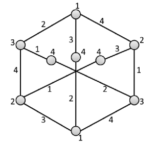
Figure 2: 4-total-colouring of the Petersen graph minus one vertex.

Now, suppose that $G$ is obtained from the Heawood graph by deleting one vertex (and then subdividing edges incident to at least one degree-2 vertex). This means that the reduced graph of $G$ is $H^{*}$. On Figure 3, a 4-total-coloring of $H^{*}$ is shown. Here, all branches of length 2 have a “good patern” (that is not ABAB), so Lemma 6 handles their subdivisions. But unfortunately, some paths of length 2 have a bad pattern. So, we are done when exactly one vertex is deleted, but we have to study what happens when 2 vertices are deleted.

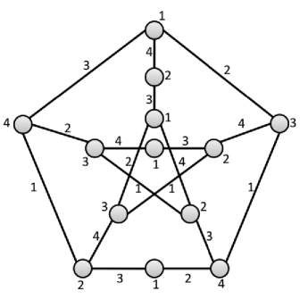
Figure 3: 4-total-colouring of the Heawood graph minus one vertex.

So, suppose that $G$ is obtained from the Heawood graph by deleting two vertices (and then subdividing edges incident to at least one degree-2 vertex). Figures 4 and 5 show the only two reduced graphs that may happen. All other cases are either isomorphic to these, or have a cutvertex. In the graph of Figure 4, a 2-extension of the Petersen graph is obtained, so we are done (to see this, consider the reduced graph, and add a vertex adjacent to the three vertices of degree 2, this gives a classical embedding of Petersen). In the graph of Figure 5, a coloring is shown.

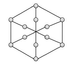
Figure 4: Heawood graph minus two vertices — a 2-extension of the Petersen graph.

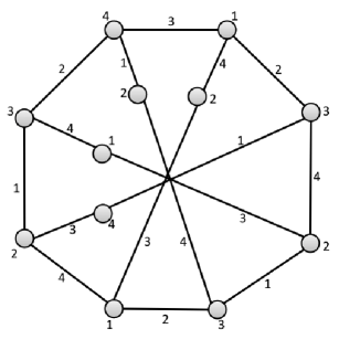
Figure 5: 4-total-colouring of the Heawood graph minus two vertices.

Now suppose that $G$ is obtained by deleting 3 vertices from the Heawood graph (and then subdividing edges incident to at least one degree-2 vertex). Since we are done in graph of Figure 4 (because all 2-extensions of the Petersen graph are already handled), we may assume that one vertex is deleted from graph of Figure 5, and up to symmetry, there is only one way to do so. This leads us to the graph of Figure 6 where a coloring is shown. Here, up to symmetries, there are two possible places for $u$ (highlighted in the figure) but the coloring handles both. Note that it is essential that all branches of length 2 have a good pattern (not ABAB). If more vertices are deleted, a 2-extension of the Petersen graph or a sparse graph is obtained.  

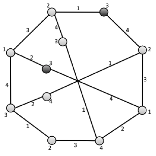
Figure 6: 4-total-colouring of the Heawood graph minus three vertices.

Proof of Theorem 5

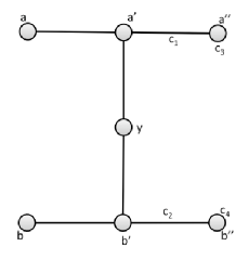
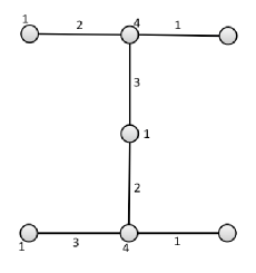
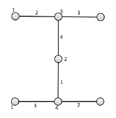
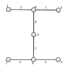
Figure 7: Several 4-colourings.

Proof: If the maximum degree of a graph is at most 2, then the graph is a disjoint union of paths and cycles, so the conclusion holds. So, let $G$ be a $\{$square,unichord$\}$-free graph of maximum degree 3 that is not a complete graph on four vertices. We shall prove that $G$ is 4-total-colourable by induction on $|V(G)|$. By Lemmas 7 and 8 this holds for sparse graphs and for 2-connected 2-extensions of the Petersen graph and the Heawood graph (in particular for the claw=$K_{1,3}$, the smallest $\{$square,unichord$\}$-free graph of maximum degree at least 3).

If $G$ has a 1-cutset with split $(X,Y,v)$, a 4-total-colouring of $G$ can be recovered from 4-total-colourings of its blocks. Hence, we suppose that $G$ is 2-connected, and we apply Theorem 3. The only outcome not handled so far is that $G$ has a proper 2-cutset with split $(X,Y,a,b)$, and we choose such a 2-cutset subject to the minimality of $|X|$. By Lemma 4, $a$ and $b$ both have two neighbors in $X$ and the block of decomposition $G_{X}$ is sparse or is a 2-extension of Petersen or Heawood graph.

Since $G$ has maximum degree 3, by Lemma 4, vertices $a,b$ both have a unique neighbor in $Y$, say $a^{\prime},b^{\prime}$ respectively. Note that $a^{\prime}\neq b^{\prime}$, for otherwise, $a^{\prime}=b^{\prime}$ would be a cutvertex of the graph (since $|Y|\geq 2$ and $a,b$ have degree 3). We claim that there exists a total-colouring of $G[Y\cup\{a,b\}]$ such that $a$ and $b$ both receive colour 1, $aa^{\prime}$ receive colour 2 and $bb^{\prime}$ receive colour 3. To prove the claim, we consider two cases.

Case 1: $Y$ contains no vertex adjacent to $a^{\prime}$ and $b^{\prime}$. This property allows us to build the block of decomposition $G_{Y}$ in a slightly unusual way: block $G_{Y}$ is obtained from $G[Y\cup\{a,b\}]$ by contracting $a$ and $b$ into a new vertex $u_{ab}$. Since $a^{\prime}\neq b^{\prime}$, this does not create a double edge. Let us check that $G_{Y}$ is $\{$square,unichord$\}$-free. Since $a$ and $b$ have each a unique neighbor in $Y$, it is easily seen that $G_{Y}$ is unichord-free. Since $G$ is square-free, a square in $G_{Y}$ must be formed by $u_{ab},a^{\prime},b^{\prime}$ and a common neighbor $a^{\prime}$ and $b^{\prime}$, a contradiction to the assumption of Case 1. Now, by the induction hypothesis, we total-colour $G_{Y}$. Up to symmetry, $u_{ab}$ receives colour 1, $u_{ab}a^{\prime}$ receive colour 2, and $u_{ab}b^{\prime}$ receive colour 3. This 4-total-colouring is also a 4-total-colouring of $G[Y\cup\{a,b\}]$ (we give colour 1 to $a$ and $b$, color 2 to $aa^{\prime}$, color 3 to $bb^{\prime}$, and the color of any other element in $G[Y\cup\{a,b\}]$ is the same as in $G_{Y}$). This completes the proof of the claim in Case 1.

Case 2: $Y$ contains a vertex $y$ adjacent to $a^{\prime}$ and $b^{\prime}$. If both $a^{\prime}$ and $b^{\prime}$ have degree 2 then $G$ is sparse. If one of $a^{\prime}$ or $b^{\prime}$ has degree 2 then this vertex is a 1-cutset of $G$. Hence we may assume that both $a^{\prime}$ and $b^{\prime}$ have degree 3. We total-colour $G[Y\setminus\{y\}]$ by the induction hypothesis, and check that vertices $a^{\prime}$ and $b^{\prime}$ can be recoloured so that the 4-total-colouring can be extended to a 4-total-colouring of $G[Y\cup\{a,b\}]$ that satisfies our constraints. We call $a^{\prime\prime}$ (resp. $b^{\prime\prime}$) the unique neighbour of $a^{\prime}$ in $Y$ that is not $y$ or $a$ (resp. $b$). We suppose that $a^{\prime}a^{\prime\prime}$, $b^{\prime}b^{\prime\prime}$, $a^{\prime\prime}$ and $b^{\prime\prime}$ receive colours $c_{1}$, $c_{2}$, $c_{3}$, $c_{4}$ respectively, see Figure 7.

If $c_{1}=c_{2}$, say $c_{1}=c_{2}=1$, then $|\{c_{1},c_{2},c_{3},c_{4}\}|\leq 3$, so at least one colour, say 4, is in $\{1,2,3,4\}\setminus\{c_{1},c_{2},c_{3},c_{4}\}$. We may use this colour to recolour $a^{\prime}$ and $b^{\prime}$, and the 4-total-colouring can be extended as in Figure 7. So, from here on, we suppose $c_{1}\neq c_{2}$, say $c_{1}=1$ and $c_{2}=2$.

If $c_{3}\neq c_{4}$, then up to a relabelling of the colours, we may recolour $a^{\prime}$ and $b^{\prime}$ with colours $3$ and $4$ respectively. Indeed, this can be checked when $\{c_{3},c_{4}\}$ is any of $\{1,2\}$, $\{1,3\}$, …, $\{3,4\}$. Then the 4-total-colouring can be extended as in Figure 7.

Finally, we may assume $c_{3}=c_{4}$, say $c_{3}=c_{4}=3$. In this case, the 4-total-colouring can be extended as in Figure 7. This completes the proof of the claim in Case 2.

Now, let $G_{X}$ be defined by adding to $G[X\cup\{a,b\}]$ a vertex $u$ adjacent to $a,b$ even if $a$ and $b$ have a common neighbor (so this is not the block as defined after Theorem 1). If there is a node of $X$ whose neighborhood in $G$ is $\{a,b\}$ then $G[X\cup\{a,b\}]$ is a cycle (because of the minimality of $X$) and $G_{X}$ is sparse, and contains a square. Otherwise, $G_{X}^{\prime}=G_{X}$, so by Lemma 4, $G_{X}$ is sparse or a 2-extension of Petersen or Heawood graph. In $G_{X}$, precolour $a$ and $b$ with colour 1, $ua$ with colour 2, and $ub$ with colour 3. Apply Lemma 7 (if $G_{X}$ is sparse) or Lemma 8 (if $G_{X}$ is a 2-extension of Petersen or Heawood graph) to $G_{X}$. This gives a 4-total-colouring of $G_{X}$. A 4-total-colouring of $G$ is obtained as follows: elements of $G$ that are in $G_{X}$ receive the colour they have in $G_{X}$, and elements that are in $G[Y\cup\{a,b\}]$ receive colours as in the claim above.

References

- (1) G. Li, L. Zhang. Total chromatic number of one kind of join graphs. Discrete Math. 306 (2006) 1895–1905.
- (2) G. Li, L. Zhang. Total chromatic number of the join of and . Chinese Quart. J. Math. 21 (2006) 264–270.
- (3) A. V. Kostochka. The total coloring of a multigraph with maximal degree 4. Discrete Math. 17 (1977) 161–163.
- (4) A. V. Kostochka. The total chromatic number of any multigraph with maximum degree five is at most seven. Discrete Math. 162 (1996) 199–214.
- (5) R. C. S. Machado and C. M. H. de Figueiredo. Total chromatic number of unichord-free graphs. Discrete Appl. Math. 159 (2011) 1851–1864.
- (6) R. C. S. Machado and C. M. H. de Figueiredo. Complexity separating classes for edge-colouring and total-colouring. J. Braz. Comput. Soc. 17 DOI: 10.1007/s13173-011-0040-8.
- (7) R. C. S. Machado, C. M. H. de Figueiredo, and N. Trotignon. Edge-colouring and total-colouring chordless graphs. Available at http://perso.ens-lyon.fr/nicolas.trotignon/articles/chordless.pdf.
- (8) R. C. S. Machado, C. M. H. de Figueiredo, and K. Vušković. Chromatic index of graphs with no cycle with unique chord. Theoret. Comput. Sci. 411 (2010) 1221–1234.
- (9) C. J. H. McDiarmid, A. Sánchez-Arroyo. Total colouring regular bipartite graphs is NP-hard. Discrete Math. 124 (1994) 155–162.
- (10) M. Rosenfeld. On the total coloring of certain graphs. Israel J. Math. 9 (1971) 396–402.
- (11) A. Sánchez-Arroyo. Determining the total colouring number is NP-hard. Discrete Math. 78 (1989) 315–319.
- (12) N. Trotignon and K. Vušković. A structure theorem for graphs with no cycle with a unique chord and its consequences. J. Graph Theory 63 (2010) 31–67.
- (13) V. G. Vizing. On an estimate of the chromatic class of a -graph (in Russian). Diskret. Analiz 3 (1964) 25–30.
- (14) N. Vijayaditya. On the total chromatic number of a graph. J. London Math. Soc. (2) 3 (1971) 405–408.
- (15) W. Wang. Total chromatic number of planar graphs with maximum degree ten. J. Graph Theory 54 (2007) 91–102.
- (16) S.-D. Wang and S.-C. Pang. The determination of the total-chromatic number of series-parallel graphs. Graphs Combin. 21 (2005) 531–540.
- (17) Z. Zhang, J. Zhang, and J. Wang. Total chromatic number of some graphs. Sci. Sinica Ser. A 31 (1988) 1434–1441.