Approximate Counting CSP
Solutions Using Partition Function

Abstract

We propose a new approximate method for counting the number of the solutions for constraint satisfaction problem (CSP). The method derives from the partition function based on introducing the free energy and capturing the relationship of probabilities of variables and constraints, which requires the marginal probabilities. It firstly obtains the marginal probabilities using the belief propagation, and then computes the number of solutions according to the partition function. This allows us to directly plug the marginal probabilities into the partition function and efficiently count the number of solutions for CSP. The experimental results show that our method can solve both random problems and structural problems efficiently.

1 Introduction

Counting the number of solutions for constraint satisfaction problem, denoted by #CSP, is a very important problem in Artificial Intelligence (AI). In theory, #CSP is a #P-complete problem even if the constraints are binary, which has played a key role in complexity theory. In practice, effective counters have opened up a range of applications, involving various probabilistic inferences, approximate reasoning, diagnosis, and belief revision.

In recent years, many attentions have been focused on counting a specific case of #CSP, called #SAT. By counting components, Bayardo and Pehoushek presented an exact counter for SAT, called Relsat [1]. By combining component caching with clause learning together, Sang et al. created an exact counter cachet [2]. Based on converting the given CNF formula into d-DNNF form, which makes the counting easily, Darwiche introduced an exact counter c2d [3]. By introducing an entirely new approach of coding components, Thurley addressed an exact counter sharpSAT [4]. By using more reasoning, Davies and Bacchus addressed an exact counter #2clseq [5]. Besides the emerging exact #SAT solvers, Wei and Selman presented an approximate counter ApproxCount for SAT by using Markov Chain Monte Carlo (MCMC) sampling [6]. Building upon ApproxCount, Gomes et al. used sampling with a modified strategy and proposed an approximate counter SampleCount [7]. Relying on the properties of random XOR constraints, an approximate counter MBound was introduced in [8]. Using sampling of the backtrack-free search space of systematic SAT solver, SampleMinisat was addressed in [9]. Building on the framework of SampleCount, Kroc et al. exploited the belief propagation method and presented an approximate counter BPCount [10]. By performing multiple runs of the MiniSat SAT solver, Kroc et al. introduced an approximate counter, called MiniCount [10].

Recently, more efforts have been made on the general #CSP problems. For example, Angelsmark et al. presented upper bounds of the #CSP problems [11]. Bulatov and Dalmau discussed the dichotomy theorem for the counting CSP [12]. Pesant exploited the structure of the CSP models and addressed an algorithm for solving #CSP [13]. Dyer et al. considered the trichotomy theorem for the complexity of approximately counting the number of satisfying assignments of a Boolean CSP [14]. Yamakami studied the dichotomy theorem of approximate counting for complex-weighted Boolean CSP [15]. Though great many studies had been made on the algorithms for the #CSP problems, only a few of them related to the #CSP solvers. Gomes et al. proposed a new generic counting technique for CSPs building upon on the XOR constraint [16]. By adapting backtracking with tree-decomposition, Favier et al. introduced an exact #CSP solver, called #BTD [17]. In addition, by relaxing the original CSP problems, they presented an approximate method Approx #BTD [17].

In this paper, we propose a new type of method for solving #CSP problems. The method derives from the partition function based on introducing the free energy and capturing the relationship of probabilities of variables and constraints. When computing the number of the solutions of a given CSP formula according to the partition function, we require the marginal probabilities of each variable and each constraint to plug into the partition function. In order to obtain the marginal probabilities, we employ the belief propagation (BP) because it can organize a computation that makes the marginal probabilities computing tractable and eventually returns the marginal probabilities. In addition, unlike the counter BPCount using the belief propagation method for obtaining the information deduced from solution samples in SampleCount, we employ the belief propagation method for acquiring information for partition function. This leads to two differences between BPCount and our counter. The first one is the counter BPCount requires to iteratively perform the belief propagation method and repeatedly obtain the marginal probabilities of each variable on the simplified SAT formulae; while our counter carries out the belief propagation method only once, which spends less cost. The second one is that the two counters obtaining the exact number of solutions depending on different circumstances. The counter BPCount needs the corresponding factor graphs of the simplified SAT formulae all have no cycles; while our counter only needs the factor graph of the given CSP formula has no cycle, which meets easily.

Our experiments reveal that our counter for CSP, called PFCount, works quite well. We consider various hard instances, including the random instances and the structural instances. For the random instances, we consider the instances based on the model RB close to the phase transition point, which has been proved the existence of satisfiability phase transition and identified the phase transition points exactly. With regard to the random instances, our counter PFCount improves the efficiency tremendously especially for instances with more variables. Moreover, PFCount presents a good estimate to the number of solutions for instances based on model RB, even if the instances scales are relatively large. Therefore, the effectiveness of PFCount is much more evident especially for random instances. For the structural instances, we focus on the counting problem based on graph coloring. The performance of PFCount for solving structural instances is in general comparing with the random instances because PFCount sometimes can’t converge. However, once PFCount can converge, it can estimate the number of the solutions of instances efficiently. As a whole, PFCount is a quite competitive #CSP solver.

2 Preliminaries

A constraint satisfaction problem (CSP) $\mathcal{P}$ is defined as a pair $\mathcal{P}=\langle V,C\rangle$, where $V=\{x_{1},x_{2},...,x_{n}\}$ is a set of variables and $C=\{c_{1},c_{2},...,c_{m}\}$ is a set of constraints defined on V. For each variable $x_{i}$ in V, the domain $D_{i}$ of $x_{i}$ is a set with $|D_{i}|$ values; the variable $x_{i}$ can be only assigned a value from $D_{i}$. A constraint c, called a k-ary constraint, consists of k variables $x_{c_{1}},x_{c_{2}},...,x_{c_{k}}$ and a relation $R\subseteq D_{c_{1}}\times D_{c_{2}}\times...\times D_{c_{k}}$, where $c_{1}$, $c_{2}$, …, $c_{k}$ are distinct. The relation $R$ specifies all the allowed tuples of values for the variables $x_{c_{1}},x_{c_{2}},...,x_{c_{k}}$ which are compatible with each other. The variable configuration of a CSP $\mathcal{P}$ is $X=\{x_{1}=d_{1},x_{2}=d_{2},...,x_{n}=d_{n}\}$ that assigns each variable a value from its domain. A solution to a constraint $c_{i}$ is a variable configuration $X_{c_{i}}=\{x_{c_{1}}=d_{c_{1}},x_{c_{2}}=d_{c_{2}},...,x_{c_{k}}=d_{c_{k}}\}$ that sets values to each variable in the constraint $c_{i}$ such that $X_{c_{i}}\in R_{i}$. We also say that the variable configuration $X_{c_{i}}$ satisfies the constraint $c_{i}$. A solution to a CSP $\mathcal{P}$ is a variable configuration such that all the constraints in C are satisfied. Given a CSP $\mathcal{P}$, the decision problem is to determine whether the CSP $\mathcal{P}$ has a solution. The corresponding counting problem (#CSP) is to determine how many solutions the CSP $\mathcal{P}$ has.

A CSP $\mathcal{P}$ can be expressed as a bipartite graph called factor graph (see Fig. 1). The factor graph has two kinds of nodes, one is variable node (which we draw as circles) representing the variables, and the other is function node (which we draw as squares) representing the constraints. A function node is connected to a variable node by an edge if and only if the variable appeares in the constraint. In the rest of this paper, we will always index variable nodes with letters starting with i, and factor nodes with letters starting with $c_{i}$. In addition, for every variable node i, we will use V(i) to denote the set of function nodes which it connects to, and V(i)$\setminus c_{i}$ to denote the set V(i) without function node $c_{i}$. Similarly, for each function node $c_{i}$, we will use V($c_{i}$) to denote the set of variable nodes which it connects to, and V($c_{i}$)$\setminus$ i to denote the set V($c_{i}$) without variable node i.

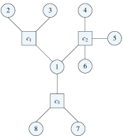
Figure 1: An example of a factor graph with 8 variable nodes i=1, 2, …, 8 and 3 function nodes $c_{1},c_{2},c_{3}$. The CSP $\mathcal{P}$ is encoded as $\mathcal{P}=\langle\{x_{1},x_{2},...,x_{8}\},\{c_{1}=(x_{1}<x_{2}<x_{3}),c_{2}=(x_{1}\neq x_{4}\neq x_{5}\neq x_{6}),c_{3}=(x_{1}+x_{7}+x_{8}<10)\}\rangle$, where V($c_{1}$) = {1, 2, 3}, V($c_{2}$) = {1, 4, 5, 6}, V($c_{3}$) = {1, 7, 8}.

3 Partition Function for Solving #CSP

In this section, we present a new approximate approach, called PFCount, for counting the number of solutions for constraint satisfaction problem. The approach derives from the partition function based on introducing the free energy and capturing the relationship of probabilities of variables and constraints. In the following, we will describe the partition function in details.

3.1 Partition Function for Counting

In this subsection, we present a partition function for counting the number of solutions for CSP. The partition function is an important quantity in statistical physics, which describes the statistical properties of a system. Most of the aggregate thermodynamic variables of the system, such as the total energy, free energy, entropy, and pressure, can be expressed in terms of the partition function. To facilitate the understanding, we first describe the notion of the partition function. Given a system of n particles, each of which can be in one of a discrete number of states, i.e., $d_{1},d_{2},...,d_{n}$, and a state of the system X denoted by $X=\{x_{1}=d_{1},x_{2}=d_{2},...,x_{n}=d_{n}\}$, i.e., the ith particle $x_{i}$ is in the state $d_{i}$, the partition function in statistical physics is defined as

$$Z(T)={1\over p(X)}e^{-E(X)/T}$$ (1)

where T is the temperature, E(X) is the energy of the state X, and p(X) is the probability of the state X. In this paper, we focus on the partition function that the temperature T is assigned to 1.

Since the partition function is also used in probability theory, in the following we will learn the partition function from the probability theory. Given a CSP $\mathcal{P}$ and a variable configuration $X=\{x_{1}=d_{1},x_{2}=d_{2},...,x_{n}=d_{n}\}$ of $\mathcal{P}$, the partition function in probability theory is defined in Equation (2).

$$Z={1\over p(X)}\prod_{i=1}^{m}f_{c_{i}}(X)$$ (2)

where p(X) is the the joint probability distribution, function $f_{c_{i}}(X)$ is a Boolean function range {0, 1}, which evaluates to 1 if and only if the constraint $c_{i}$ is satisfied, evaluates to 0 otherwise; and m is the number of constraints. Based on Equation (2), the joint probability distribution p(X) over the n variables can be expressed as the follows.

$$p(X)={1\over Z}\prod_{i=1}^{m}f_{c_{i}}(X)$$ (3)

Because the construction of the joint probability distribution is uniform over all variable configurations, Z is the number of solutions of the given CSP $\mathcal{P}$. Therefore, #CSP can be solved by computing a partition function. In the following, we will propose the derivation of the partition function.

In order to present a calculation method to compute the partition function, we introduce the variational free energy defined by

$$F(b(X))=\sum_{X}b(X)E(X)+\sum_{X}b(X)\ln b(X)$$ (4)

where E(X) is the energy of the state X and b(X) is a trial probability distribution. Simplifying the Equation (4), we draw up the following equation.

$$F(b(X)) = \sum_{X}b(X)E(X)+\sum_{X}b(X)\ln b(X)$$ (5)

$$= \sum_{X}b(X)\ln(e^{E(X)}b(X))$$

$$= \sum_{X}b(X)\ln{b(X)\over e^{-E(X)}}$$

By setting T to 1 in Equation (1), we can obtain:

$$e^{-E(X)}=p(X)Z$$ (6)

Then we take the Equation (6) into (5) and acquire:

$$F(b(X)) = \sum_{X}b(X)\ln{b(X)\over p(X)Z}$$ (7)

$$= \sum_{X}b(X)(\ln{b(X)\over p(X)}-\ln Z)$$

$$= -\ln Z\sum_{X}b(X)+\sum_{X}b(X)\ln{b(X)\over p(X)}$$

Since b(X) is a trial probability distribution, the sum of the probability distribution should be 1, i.e. $\sum_{X}b(X)=1$. Then the Equation (7) can be expressed as the follows.

$$F(b(X))=-\ln Z+\sum_{X}b(X)\ln{b(X)\over p(X)}$$ (8)

By analyzing the Equation (8), we know that the second term is equal to zero if b(X) is equal to p(X). So when b(X) is equal to p(X), the partition function can be written as

$$Z=\exp(-F(p(X)))$$ (9)

Then by taking the Equation (4) into the above equation, we obtain

$$Z=\exp(-\sum_{X}p(X)E(X)-\sum_{X}p(X)\ln p(X))$$ (10)

For a factor graph with no cycles, p(X) can be easily expressed in terms of the marginal probabilities of variables and constraints as the follows.

$$p(X)=\prod_{i=1}^{m}p_{c_{i}}(X_{c_{i}})\prod_{j=1}^{n}p_{j}(d_{j})^{1-\sigma_{j}}$$ (11)

where $\sigma_{j}$ is the number of times that the variable $x_{j}$ occurs in the constraints, m and n are the number of constraints and variables respectively, $p_{c_{i}}(X_{c_{i}})$ and $p_{j}(d_{j})$ are the marginal probabilities of constraints and variables respectively.

In addition, by analyzing the two partition functions presented in equations (1) and (2), we can see that p(X) and Z are equal when T is set to 1. Thus, we can obtain the following equation from Equation (1) and Equation (2) on account of the equivalents Z and p(X).

$$E(X)=-\ln\prod_{i=1}^{m}f_{c_{i}}(X)=-\sum_{i=1}^{m}\ln f_{c_{i}}(X)$$ (12)

Then the partition function can be expressed as the follows by plugging the Equation (11) and Equation (12) into Equation (10).

$$Z=\exp (-\sum_{X}(\prod_{i=1}^{m}p_{c_{i}}(X_{c_{i}})(\prod_{j=1}^{n}p_{j}(d_{j})^{1-\sigma_{j}})(-\sum_{i=1}^{m}\ln f_{c_{i}}(X_{c_{i}})))$$ (13)

$$-\sum_{X}(\prod_{i=1}^{m}p_{c_{i}}(X_{c_{i}})\prod_{j=1}^{n}p_{j}(d_{j})^{1-\sigma_{j}})\ln(\prod_{i=1}^{m}p_{c_{i}}(X_{c_{i}})\prod_{j=1}^{n}p_{j}(d_{j})^{1-\sigma_{j}}))$$

In Equation (13), when the variable configuration X is a solution to a CSP $\mathcal{P}$, the function $f_{c_{i}}(X_{c_{i}})$ is assigned 1, which means that the term $-\sum_{i=1}^{m}\ln f_{c_{i}}(X_{c_{i}})$ evaluates to 0. On the other hand, when the variable configuration X is not a solution to a CSP $\mathcal{P}$, the term $\prod_{i=1}^{m}p_{c_{i}}(X_{c_{i}})$ evaluates to 0. Therefore, whether or not the variable configuration X is a solution to a CSP $\mathcal{P}$, the first term in the exponential function must evaluate to 0. Then Equation (13) can be expressed as the follows.

$$Z= \exp(-\sum_{X}(\prod_{i=1}^{m}p_{c_{i}}(X_{c_{i}})\prod_{j=1}^{n}p_{j}(d_{j})^{1-\sigma_{j}})\ln(\prod_{i=1}^{m}p_{c_{i}}(X_{c_{i}})\prod_{j=1}^{n}p_{j}(d_{j})^{1-\sigma_{j}}))$$ (14)

$$= \exp(-\sum_{i=1}^{m}\sum_{X_{c_{i}}}p_{c_{i}}(X_{c_{i}})\ln p_{c_{i}}(X_{c_{i}})-\sum_{j=1}^{n}(1-\sigma_{j})\sum_{d_{j}}p_{j}(d_{j})\ln p_{j}(d_{j}))$$

From the above equation, we can learn that the number of solutions of a given CSP $\mathcal{P}$ can be calculated according to the partition function if the marginal probability of variable $p_{j}(d_{j})$ and the marginal probability of constraint $p_{c_{i}}(X_{c_{i}})$ can be obtained. In the following, we will present an approach to compute the marginal probabilities.

3.2 Marginal Probabilities Estimate Using BP

In this subsection, we address a method BP to calculate the marginal probabilities. The belief propagation, BP for short, is a message passing procedure, which is a method for computing marginal probabilities [18]. The BP procedure obtains exact marginal probabilities if the factor graph of the given CSP $\mathcal{P}$ has no cycles, and it can still empirically provide good approximate results even when the corresponding factor graph does have cycles.

Figure 2: The BP procedure.

To describe the BP procedure, we first introduce messages between function nodes and their neighboring variable nodes and vice versa. The message $p_{c_{i}\rightarrow i}(d_{i})$ passed from a function node $c_{i}$ to one of its neighboring variable nodes i can be interpreted as the probability of constraint $c_{i}$ being satisfied if the variable $x_{i}$ takes the value $d_{i}\in D_{i}$; while the message $p_{i\rightarrow c_{i}}(d_{i})$ passed from a variable node i to one of its neighboring function nodes $c_{i}$ can be interpreted as the probability that the variable $x_{i}$ takes the special value $d_{i}\in D_{i}$ in the absence of constraint $c_{i}$. Next we concentrate on presenting the details of the BP procedure (see Fig. 2). At first, the message $p_{c_{i}\rightarrow i}(d_{i})\in[0,1]$ is initialized for every edge ($c_{i}$, i) and every value $d_{i}\in D_{i}$. Then the messages are updated with the following equations.

$$p_{i\rightarrow c_{i}}^{(t)}(d_{i})=C_{i\rightarrow c_{i}}\prod_{c_{j}\in V(i)\setminus c_{i}}p_{c_{j}\rightarrow i}^{(t-1)}(d_{i})$$ (15)

$$p_{c_{i}\rightarrow i}^{(t)}(d_{i})=\sum_{d_{j}\in D_{j},j\in V(c_{i})\setminus i}f_{c_{i}}(X_{c_{i}})\prod_{j\in V(c_{i})\setminus i}p_{j\rightarrow c_{i}}^{(t-1)}(d_{i})$$ (16)

where $C_{i\rightarrow c_{i}}$ is a normalization constant ensuring that $p_{i\rightarrow c_{i}}(d_{i})$ is a probability, and $f_{c_{i}}(X_{c_{i}})$ is a characteristic function taking the value 1 if the variable configuration $X_{c_{i}}$ satisfies the constraint $c_{i}$, taking the value 0 otherwise. The BP procedure runs the equations (15) and (16) iteratively until the message $p_{c_{i}\rightarrow i}(d_{i})$ converges for every edge ($c_{i}$, i) and every value $d_{i}\in D_{i}$. When they have converged, we can then calculate the marginal probabilities of each variable and each constraint in the following equations.

$$p_{i}(d_{i})=C^{\prime}\prod_{c_{i}\in V(i)}p_{c_{i}\rightarrow i}(d_{i})$$ (17)

$$p_{c_{i}}(X_{c_{i}})=C\texttt{"}\prod_{i\in V(c_{i})}\prod_{c_{j}\in V(i)\setminus c_{i}}p_{c_{j}\rightarrow i}(d_{i})$$ (18)

where C’ and C" are normalization constants ensuring that $p_{i}(d_{i})$ and $p_{c_{i}}(X_{c_{i}})$ are probabilities, and $f_{c_{i}}(X_{c_{i}})$ is a characteristic function taking the value 1 if the variable configuration $X_{c_{i}}$ satisfies the constraint $c_{i}$, taking the value 0 otherwise.

As a whole, the BP procedure organizes a computation that makes the marginal probabilities computing tractable and eventually returns the marginal probabilities of each variable and each constraint which can be used in the partition function. As we know, the BP procedure can present exact marginal probabilities if the factor graph of the given CSP $\mathcal{P}$ has no cycle. And from the whole derivation of the partition function, we understand that all equations address exact results if the factor graph is a tree. Thus, we obtain the following theorem.

3.2.1 Theorem 1

The method PFCount provides an exact number of solutions for a CSP $\mathcal{P}$ if the factor graph of the given CSP $\mathcal{P}$ has no cycle.

The above theorem illustrates that PFCount can present an exact number of solutions if the corresponding factor graph of the given CSP $\mathcal{P}$ has no cycle. In addition, even when the factor graph does have cycles, our method still empirically presents good approximate number of solutions for CSP.

4 Experimental Results

In this section, we perform two experiments on a cluster of 2.4 GHz Intel Xeon machines with 2 GB memory running Linux CentOS 5.4. The purpose of the first experiment is to demonstrate the performance of our method on random instances; the second experiment is to compare our method with two other methods on structural instances. Our #CSP solver is implemented in C++, which we also call PFCount. For each instance, the run-time is in seconds and the timeout limit is 7200s.

4.1 Evaluation on the Random Instances

In this subsection, we conduct experiments on CSP benchmarks of model RB, which can provide a framework for generating asymptotically hard instances so as to give a challenge for experimental evaluation of the #CSP solvers [19]. The benchmarks of model RB is determined by parameters (k, n, $\alpha$, r, p), where k denotes the arity of each constraint; n denotes the number of variables; $\alpha$ determines the domain size $d=n^{\alpha}$ of each variable; r determines the number $m=rn\ln n$ of constraints; p determines the number $t=pd^{k}$ of disallowed tuples of each relation.

4.1.1 Comparing PFCount with State-of-the-Art Counters

Table 1: Comparison of counters on CSP benchmarks of model RB (- represents out of time and times are in seconds).

Table 1 illustrates the comparison of PFCount with state-of-the-art exact #SAT solvers sharpSAT, c2d, cachet, and approximate solvers ApproxCount, BPCount on CSP benchmarks of model RB close to the phase transition point. In the experiment, we choose random instances $\mathcal{P}\in$ (2, n, 0.8, 3, p) with n $\in$ {10, 20, 30, 40}. Moreover, since the theoretical phase transition point $p\approx$ 0.23 for k = 2, $\alpha$ = 0.8, r = 3, n $\in$ {10, 20, 30, 40}, we set p = 0.20. In Table 1, the instance frba-b-c represents the instance containing a variables, owning a domain with b values for each variable, and indexing c; ExactS represents the exact number of solutions of each instance; AppS represents the approximate number of solutions of each instance. Note that the exact number of solutions of each instance is obtained by the exact #SAT solvers and the CSP instances solved by these #SAT solvers are translated into SAT instances using the direct encoding method. The results reported in Table 1 suggest that the effectiveness of PFCount is much more evident especially for larger instances. For example, the efficiency of solving instances with 30 variables has been raised at least 74 times (instance frb30-15-1). And the instances with 40 variables can be solved by PFCount in a few seconds. Furthermore, PFCount presents a good estimate to the number of solutions for CSP benchmarks of model RB. Even if the instances scales are relatively large, the estimates are found to be over 63.129% correct except the instance frb20-11-3. Therefore, this experiment shows that PFCount is quite competitive compared with the other counters.

4.1.2 Evaluation the Performance of PFCount on Hard Instances

Table 2: Evaluation the performance of PFCount on hard CSP instances (all times are in seconds).

Table 2 presents the performance of our counter PFCount on hard instances based on model RB. These instances provide a challenge for experimental evaluation of the CSP solvers. In the 1st international CSP solver competition in 2005, these instances can’t be solved by all the participating CSP solvers in 10 minutes. In the recent CSP solver competition, only one solver can solve the instances frb50-23-1, frb50-23-4, frb50-23-5, frb53-24-5, frb56-25-5, and frb59-26-5; only two solvers can solve the instance frb53-24-3; four solvers can solve the instance frb53-24-1; and the rest of instances still can’t be solved in 10 minutes. In Table 2, AppS represents the approximate number of solutions of each instance; ExpectedS represents the expected number of solutions of each instance, which can be calculated as the following according to the definition of model RB [19].

$$ExpectedS=n^{\alpha n}(1-p)^{rn\ln n}$$ (19)

where n denotes the number of variables; $\alpha$ determines the domain size $d=n^{\alpha}$ of each variable; r determines the number $m=rn\ln n$ of constraints; p determines the number $t=pd^{k}$ of disallowed tuples of each relation. When n tends to infinite, ExpectedS is the number of solutions of the instances based on model RB. Empirically, when n is not very large, ExpectedS and the exact number of solutions are in the same order of magnitude. Therefore, ExpectedS precisely estimates the number of solutions of the instances based on model RB. By analyzing the results in Table 2, we can see that PFCount efficiently estimates the number of solutions of these hard CSP instances. It should be pointed out that our PFCount is only capable of estimating the numbers of solutions rather enumerating the solutions.

4.2 Evaluation on the Structural Instances

In this subsection, we carry out experiments on graph coloring instances from the DIMACS benchmark set. The #CSP solvers compared with PFCount are ILOG Solver 6.3 [20] and CSP+XORs. Table 3 illustrates the results of the comparison of the #CSP solvers on graph coloring instances. In this table, AppS is the approximate number of solutions of each instance; ExactS is the exact number of solutions of each instance calculated by the exact counters. Note that the results presented by the ILOG Solver and CSP+XORs are based on [16] for lack of the binary codes. As can be seen from Table 3, PFCount doesn’t give good estimate on these structural instances in contrast with the random instances. However, the run-time of PFCount clearly outperforms other #CSP solvers greatly.

Table 3: Comparison of #CSP solvers on graph coloring instances (- represents out of time and times are in seconds).

5 Conclusion

This paper addresses a new approximate method for counting the number of solutions for constraint satisfaction problem. It first obtains the marginal probabilities of each variable and constraint by the belief propagation approach, and then computes the number of the solutions of a given CSP formula according to a partition function, which obtained by introducing the free energy and capturing the relationship between the probabilities of the variables and the constraints. The experimental results also show that the effectiveness of our method is much more evident especially for larger instances close to the phase transition point.

References

- [1] Bayardo, R. J., and Pehoushek, J. D.: Counting models using connected components. In: 17th National Conference on Artificial Intelligence, pp. 157–162. AAAI Press, U.S. (2000)
- [2] Sang, T., Bacchus, F., Beame, P., Kautz, H. A., and Pitassi, T.: Combining component caching and clause learning for effective model counting.In: 7th Theory and Applications of Satisfiability Testing. Springer, Heidelberg (2004)
- [3] Darwiche, A.: New advances in compiling CNF into decomposable negation normal form. In: 16th European Conference on Artificial Intelligence, pp. 328–332. IOS Press, Washington (2004)
- [4] Thurley, M.: sharpSAT - counting models with advanced component caching and implicit BCP. In: 9th Theory and Applications of Satisfiability Testing, pp. 424–429. Springer, Heidelberg (2006)
- [5] Davies, J., and Bacchus, F.: Using more reasoning to improve #SAT solving. In: 22nd National Conference on Artificial Intelligence, pp. 185–190. AAAI Press, U.S. (2007)
- [6] Wei, W., and Selman, B.: A new approach to model counting. In: 8th Theory and Applications of Satisfiability Testing, pp. 324–339. Springer, Heidelberg (2005)
- [7] Gomes, C. P., Hoffmann, J., Sabharwal, A., and Selman, B.: From sampling to model counting. In: 20th International Joint Conference on Artificial Intelligence, pp. 2293–2299. Springer, Heidelberg (2007)
- [8] Gomes, C. P., Sabharwal, A., and Selman, B.: Model counting: A new strategy for obtaining good bounds. In: 21st National Conference on Artificial Intelligence, pp. 54–61. AAAI Press, U.S. (2006)
- [9] Gogate, V., and Dechter, R.: Approximate counting by sampling the backtrackfree search space. In: 22nd National Conference on Artificial Intelligence, pp. 198–203. AAAI Press, U.S. (2007)
- [10] Kroc, L., Sabharwal, A., and Selman, B.: Leveraging belief propagation, backtrack search, and statistics for model counting. In: 5th Integration of AI and OR Techniques in Contraint Programming for Combinatorial Optimzation Problems, pp. 127–141. Springer, Heidelberg (2008)
- [11] Angelsmark, O., Jonsson, P., Linusson, S., and Thapper J.: Determining the number of solutions to binary CSP instances. In: 8th Principles and Practice of Constraint Programming, pp. 327–340. Springer, Heidelberg (2002)
- [12] Bulatov, A., Dalmau, V.: Towards a dichotomy theorem for the counting constraint satisfaction problem. In: 44th Annual IEEE Symposium on Foundations of Computer Science, pp. 562–571. IEEE Computer Society, Los Alamitos, CA (2003)
- [13] Pesant, G.: Counting solutions of CSPs: a structural approach. In: International Joint Conference on Artificial Intelligence, pp. 260–266. Springer, Heidelberg (2005)
- [14] Dyera, M., Goldbergb, L. A., Jerrum, M.: An approximation trichotomy for Boolean #CSP. J. Comput. Syst. Sci. 76(3-4), 267–277 (2010)
- [15] Yamakami, T.: Approximate counting for complex-weighted Boolean constraint satisfaction problems. Inf. Comput. 219, 17–38 (2012)
- [16] Gomes, C. P., Hoeve, W. J., Sabharwal, A., and Selman, B.: Counting CSP Solutions Using Generalized XOR Constraints. In: National Conference on Artificial Intelligence, pp. 204–209. AAAI Press, U.S. (2007)
- [17] Favier, A., Givry, S., Jegou, P.: Exploiting problem structure for solution Counting. In: Principles and Practice of Constraint Programming, pp. 335–343. Springer, Heidelberg (2009)
- [18] Zhang, P., Ramezanpour, A., Zdeborova, L., and Zecchina, R.: Message passing for quantified Boolean formulas. J. Stat. Mech-Theory E. pp. 05025 (2012)
- [19] Xu, K., Boussemart, F., Hemery, F., and Lecoutre C.: Random constraint satisfaction: Easy generation of hard (satisfiable) instances. Artif. Intell. 171(8-9), 514–534 (2007)
- [20] ILOG, SA. 2006. ILOG Solver6.3 reference manual.