Construction of KP solitons from wave patterns

Abstract

We often observe that waves on the surface of shallow water form complex web-like patterns. They are examples of nonlinear waves, and these patterns are generated by nonlinear interactions among several obliquely propagating waves. In this note, we discuss how to construct an exact soliton solution of the KP equation from such web-pattern of shallow water wave. This can be regarded as an “inverse problem” in the sense that by measuring certain metric data of the solitary waves in the given pattern, it is possible to construct an exact KP soliton solution which can describe the non-stationary dynamics of the pattern.

1 Introduction

At any beach with flat or nearly flat bottom, one often observes interesting wave patterns as shown in Figure 1.1. In this paper, we provide a mathematical analysis for those patterns (non-stationary in general) based on the Kadomtsev-Petviashvili (KP) equation [9] which is given by

$$(4u_{t}+6uu_{x}+u_{xxx})_{x}+3u_{yy}=0.$$ (1.1)

Here $u=u(x,y,t)$ represents the normalized wave amplitude at the point $(x,y)$ in the $xy$-plane for fixed time $t$.

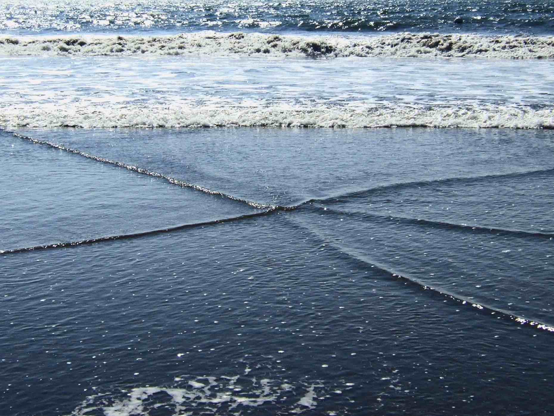
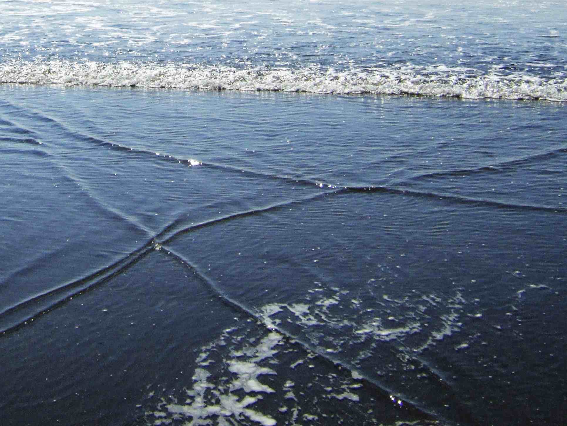
Figure 1.1: Wave patterns on a beach at Nuevo Vallarta, Mexico. Photographs by M. J. Ablowitz

From a physical perspective, the KP equation is derived from the three-dimensional Euler equations for an irrotational and incompressible fluid under the assumptions that it describes the propagation of small amplitude, long wavelength, uni-directional waves with small transverse variation (i.e., quasi-two-dimensional waves). An example of such wave phenomena observed in nature is the surface wave patterns in shallow water on long, flat beaches as shown in Figure 1.1. On a smaller scale, such wave patterns can be easily demonstrated in table-top experiments [13] (see also movies available at the website http://www.needs-conferences.net/2009/), as well as recreated in more accurate water tank experiments in the laboratory [16, 23].

The KP equation admits an important class of solitary wave solutions that are regular, non-decaying and localized along distinct lines in the $xy$-plane. These are known as the line-soliton solutions which have been studied extensively in recent years by the authors who have provided a complete classification of these solutions using geometric and combinatorial techniques [5, 6, 7, 11]. In principle, these solutions may have arbitrary number of asymptotic line solitons in the far-field and a complex interaction pattern of intermediate solitons resembling a web-like structure in the near-field region. Because of this, we sometimes call the line-soliton solutions the web-solitons. Several simple yet exact web-solitons, for example, the Y-shape soliton and several other solutions with two asymptotic solitons for $|y|\gg 0$, have been experimentally demonstrated. Indeed, in recent laboratory wave tank experiments by Harry Yeh’s group at Oregon State University surface wave patterns generated by solitary wave interactions which are very good approximations of the exact KP solutions, have been observed [16, 23].

The purpose of this note is to study the inverse problem, i.e., to construct an exact line-soliton solution of the KP equation that approximates an observed wave pattern. Specifically, we consider the wave patterns observed in shallow water such as in Figure 1.1. We assume that these patterns satisfy the assumptions stated above, necessary to derive the KP equation from the Euler equations. Then the inverse problem determines the information required to construct the exact line-soliton solution from the wave pattern data consisting of the amplitude and slopes of the solitary waves, and the locations of those waves on the $xy$-plane for fixed $t$. We emphasize at the very outset that in this note we limit our considerations only to the comparison between the wave patterns and the exact KP theory, that is, we do not take into account any higher order corrections to the KP equation due to large amplitude, finite angle (departure from quasi-two-dimensionality), uneven bottom or any such physical perturbations. In this sense, the inverse problem considered here should be regarded as a leading order approximation.

Recent interest in the study of line-soliton solutions of the KP equation has generated a data bank of photographs and video recordings of patterns formed by interacting small amplitude solitary waves in shallow water on flat beaches, see for example, a recent article by Ablowitz and Baldwin [1] and additional resources at the authors’ websites [2]. In this paper we propose an algorithm to construct the line-soliton solutions approximating those given wave patterns. Modeling of shallow water wave patterns by the line-soliton solutions are carried out in a “qualitative” fashion in the current literature (see e.g. [1, 20, 21, 22]), and at times, using ad hoc methods. Most such studies consider the KP $N$-soliton solutions given by the well-known Hirota formula [8]. But even for $N=2$, this formula is not adequate to describe the rich variety of similar interaction patterns revealed by the KP theory [5, 7] since the 2-soliton solution obtained from the Hirota formula only gives a stationary X-shape pattern. In contrast, our algorithm makes concrete quantitative use of the measurements from a given wave pattern to obtain the explicit analytical form of the KP line-soliton solution which can describe the non-stationary dynamics of the pattern.

It is important to recognize that the resonant interaction among solitary waves plays a fundamental role in the formation of surface wave patterns that can be approximated by the KP solitons. It was Miles [17, 18] who first identified the resonant interaction in KP solitons when two asymptotic line solitons of an X-shape 2-soliton solution, referred here as the X-soliton, interact obliquely at a certain critical angle, and a third soliton is created to make a Y-shape pattern. It turns out that such Y-shape wave-form is an exact solution of the KP equation, and is referred to as Y-soliton (see also [19]). Subsequently, more general type of resonant and partially-resonant line-soliton solutions have been discovered (see e.g., [4, 10, 3]). In this paper, we demonstrate using explicit examples of shallow water wave patterns that the resonant line-soliton solutions of the KP equation can be used to approximate such patterns and their dynamics fairly well.

The paper is organized as follows: In Section 2, we provide some basic background for the one-soliton solution of the KP equation, as well as the resonant Y-soliton and the non-resonant X-soliton solutions. Then in Section 3 we describe an algorithmic method to construct an exact KP soliton solution from a given wave pattern. In Section 4, we illustrate our algorithm via several explicit examples of actual shallow water wave patterns, and demonstrate that the dynamics given by the exact solutions are in good agreement with the observations. We finally give some concluding remarks in Section 5.

2 The KP solitons

Here we briefly give the background information on the KP solitons necessary to this paper and a remark on some particular solutions (see [5, 7, 11] for the details).

It is customary to prescribe the solutions of the KP equation (1.1) as

$$u(x,y,t)=2(\ln\tau)_{xx}\,,$$ (2.1)

in terms of the $\tau$-function $\tau(x,y,t)$ (see e.g. [8]). For the soliton solutions, the $\tau$-function is defined via

• $M$ distinct real parameters $\{k_{1},k_{2},\ldots,k_{M}\}$ with the ordering $k_{1}<k_{2}<\cdots<k_{M}$, and

• an $N\times M$ real matrix $A$ of full rank with $N<M$.

The explicit form of the $\tau$-function is as follows:

$$\tau(x,y,t)=\mathop{\textstyle\sum}\limits_{I}\Delta_{I}(A)\,E_{I}(x,y,t)\,,$$ (2.2)

where the sum is over all (ordered) $N$-element subsets of $[M]:=\{1,\ldots,M\}$, denoted by $\binom{[M]}{N}$ and $|I|=N$ denotes the number of elements of $I$, i.e., $I=\{i_{1}<\cdots<i_{N}\}\in\binom{[M]}{N}$. The coefficient $\Delta_{I}(A)$ is the $N\times N$ minor of the matrix $A$ with the column set $I$, and $E_{I}(x,y,t):=K_{I}\exp\Theta_{I}(x,y,t)$ where

$$K_{I}=\prod_{l>m}(k_{i_{l}}-k_{i_{m}}),\qquad\quad\Theta_{I}(x,y,t)=\mathop{\textstyle\sum}\limits_{m=1}^{N}(k_{i_{m}}x+k_{i_{m}}^{2}y-k_{i_{m}}^{3}t).$$ (2.3)

The soliton solution $u(x,y,t)$ is regular if and only if $\Delta_{I}(A)\geq 0$ for all $I\in\binom{[M]}{N}$ [14, 15]. In this case, the matrix $A$ is called a totally non-negative matrix.

In our previous works [5, 7], it was shown that the general soliton solution given by equations (2.1) and (2.2) consists of $N$ line-solitons as $y\gg 0$ and $M-N$ line-solitons as $y\ll 0$. Each of those asymptotic solitons is uniquely parametrized by a pair of distinct $k$-parameters $\{k_{i},k_{j}\}$ for $i<j$. We let $[i,j]$ denote the index pair for this soliton. Furthermore, the index pair $[i,j]$ is uniquely characterized by a map $\pi$ such that $\pi(i)=j$ if $[i,j]$ labels an asymptotic soliton for $y\gg 0$, and $\pi(j)=i$ if $[i,j]$ labels an asymptotic soliton for $y\ll 0$. The map $\pi$ turns out to be fixed-point free permutation of the index set $[M]$ known as derangement which is conveniently represented by a chord diagram as shown in examples below. Thus the soliton solution generated by the $\tau$-function (2.2) is represented by the chord diagram associated to the derangement $\pi$.

We briefly describe below some details of the one-solitons, the Y-solitons and the X-solitons which form the building blocks of a web-soliton solution of the KP equation. Those One-, Y- and X-solitons are stationary solutions of the KP equation. We emphasize that the web-solitons consisting of those solutions are no longer stationary.

2.1 One soliton solution

Asymptotic analysis of the $\tau$-function in (2.2) reveals that the solution $u(x,y,t)$ is exponentially vanishing in regions of the $xy$-plane where a single exponential $E_{I}$ is dominant over all other exponentials in (2.2) while it is localized along certain lines where a pair of dominant exponentials $E_{I},E_{J}$ are in balance. Each such line is labeled by an index pair $[i,j]$ as explained below. The solution $u(x,y,t)$ along this line is approximated by a one-soliton solution, and will be referred to as the $[i,j]$-soliton throughout this note. Along this line $[i,j]$, the $\tau$-function can be locally approximated by

$$\tau~{}\approx~{}\Delta_{I}(A)E_{I}+\Delta_{J}(A)E_{J}\,,$$

where $I=I_{0}\cup\{i\}$ and $J=I_{0}\cup\{j\}$ with $|I_{0}|=N-1$ (see [7]). Then near the line $[i,j]$, the solution $u=2(\ln\tau)_{xx}$ has the form of a one-soliton,

$$u\,\approx\,A_{[i,j]}\,\mathrm{sech}^{2}\,\Theta_{[i,j]}\,,$$ (2.4)

localized along the line $[i,j]$ given by $\Theta_{[i,j]}=0$ where

$$\Theta_{[i,j]}:=\frac{1}{2}(\Theta_{I}-\Theta_{J}) =\frac{1}{2}(k_{i}-k_{j})\left(x+\tan\Psi_{[i,j]}y-C_{[i,j]}t+x_{[i,j]}\right)$$ (2.5)

$$x_{[i,j]} =\frac{1}{k_{i}-k_{j}}\ln\frac{\Delta_{I}(A)K_{I}}{\Delta_{J}(A)K_{J}}\,.$$

(recall (2.3) for the formulae $K_{I}$ and $\Theta_{I}$). The soliton amplitude $A_{[i,j]}$, slope $\Psi_{[i,j]}$ and velocity in the positive $x$-direction $C_{[i,j]}$, are defined respectively by

$$A_{[i,j]}=\frac{1}{2}(k_{i}-k_{j})^{2},\qquad\tan\Psi_{[i,j]}={k_{i}+k_{j}},$$ (2.6)

$$C_{[i,j]}=k_{i}^{2}+k_{j}^{2}+k_{i}k_{j}>0.$$

A contour plot of this one-soliton solution is shown in Figure 2.1. Note that the angle $\Psi_{[i,j]}$ is measured counterclockwise from the $y$-axis, and $-{\textstyle\frac{\pi}{2}}<\Psi_{[i,j]}<{\textstyle\frac{\pi}{2}}$. Since the parameter $k_{i}$ appears only in the phase $\Theta_{I}$ of the exponential $E_{I}$ while $k_{j}$ appears only in $\Theta_{J}$ of the exponential $E_{J}$, the line $[i,j]$ can be viewed as representing a permutation of the index set $\{i,j\}$. That is, the parameters $k_{i}$ and $k_{j}$ are exchanged during the transition from one dominant exponential to the other by crossing the $[i,j]$-soliton. The chord diagram in Figure 2.1 depicting the exchange $k_{i}\leftrightarrow k_{j}$ represents the permutation $\pi=\left(\begin{smallmatrix}i&j\\ j&i\end{smallmatrix}\right)$ of the index set $\{i,j\}$.

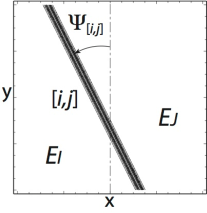
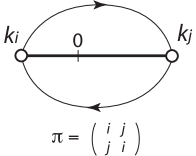
Figure 2.1: Contour plot and the chord diagram representation of the $[i,j]$-soliton

2.2 Y-soliton solution

Here we briefly describe the Y-soliton which is a system of three line solitons labeled $[i,j]$, $[j,l]$ and $[i,l]$ with $i<j<l$, interacting at a trivalent vertex. Writing each of the solitons in the form of a traveling wave $u=\Phi(\mathbf{K}_{[a,b]}\cdot\mathbf{r}-\Omega_{[a,b]}t)$ with $\mathbf{r}=(x,y)$, the wave-vector $\mathbf{K}_{[a,b]}={\textstyle\frac{1}{2}}(k_{b}-k_{a},k_{b}^{2}-k_{a}^{2})$ and the frequency $\Omega_{[a,b]}={\textstyle\frac{1}{2}}(k_{b}^{3}-k_{a}^{3})$, the soliton triplet satisfy the resonant conditions

$$\mathbf{K}_{[i,j]}+\mathbf{K}_{[j,l]}=\mathbf{K}_{[i,l]}\,,\quad\qquad\Omega_{[i,j]}+\Omega_{[j,l]}=\Omega_{[i,l]}\,.$$

Near the trivalent vertex, the $\tau$-function has the form

$$\tau\approx~{}\Delta_{I}(A)E_{I}+\Delta_{J}(A)E_{J}+\Delta_{L}(A)E_{L}\,.$$

There are two cases for the index sets $\{I,J,L\}$ leading to the contour plots in Figures 2.2.

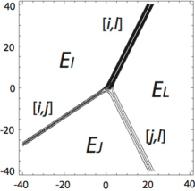
(a)                    (b) 

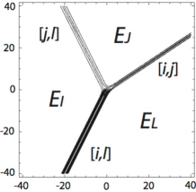
Figure 2.2: Contour plots of the Y-solitons. Resonant soliton triplet $[i,j],[j,l]$ and $[i,l]$.

• The index sets are given by $I=I_{0}\cup\{i\},J=I_{0}\cup\{j\}$ and $L=I_{0}\cup\{l\}$. In this case the $[i,l]$-soliton is above the trivalent vertex while the solitons $[i,j]$ and $[j,l]$ appear below it to form a Y -shape as shown in Figure 2.2(a). Following the transitions of the dominant exponentials clockwise in Figure 2.2(a), one recovers the permutation $\pi=\left(\begin{smallmatrix}i&j&l\\ l&j&i\end{smallmatrix}\right)$ given by the three line solitons $[i,j],\,[j,l],\,[i,l]$. The chord diagram corresponding to this permutation is shown in Figure 2.3(a).

• The index sets are $I=J_{0}\cup\{i,j\},J=J_{0}\cup\{i,l\}$ and $L=J_{0}\cup\{j,l\}$. The solution in this case is related to that of Case (a) by an inversion $(x,y,t)\to(-x,-y,-t)$ so that the solitons $[i,j]$ and $[j,l]$ appear above the trivalent vertex and the $[i,l]$-soliton appears below it. The line solitons for this Y shape represent the permutation $\pi=\left(\begin{smallmatrix}i&j&l\\ j&l&i\end{smallmatrix}\right)$ as shown by the chord diagram in Figure 2.3(b).

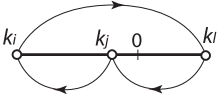
(a)                    (b) 

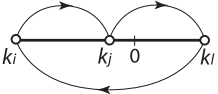
Figure 2.3: Chord diagrams for the Y-solitons in Figure 2.2. The horizontal line gives the coordinate of the $k$-parameters, i.e. $k_{i}<k_{j}<0<k_{l}$ in those diagrams.

Due to the ordering $k_{i}<k_{j}<k_{l}$, the $[i,l]$-soliton has the largest amplitude $A_{[i,l]}={\textstyle\frac{1}{2}}(k_{l}^{2}-k_{j}^{2})$, and the $[j,l]$-soliton has the largest slope $\tan\Psi_{[j,l]}=k_{j}+k_{l}$, while the $[i,j]$-soliton has the smallest slope. Note that all these information can be gathered directly from the chord diagrams presented in Figure 2.3, which is one of the main reasons we use the chord diagrams in our analysis. One should also note that the $k$-parameters in the Y-soliton are uniquely determined only from the slopes of the three solitons. Recall that the slopes of the solitons $[i,j],\,[j,l],\,[i,l]$ are respectively given by

$$\tan\Psi_{[i,j]}=k_{i}+k_{j},\quad\tan\Psi_{[j,l]}=k_{j}+k_{l},\quad\tan\Psi_{[i,l]}=k_{i}+k_{l}\,.$$

Then one can compute the values of the $k$-parameters as

$$k_{i} ={\textstyle\frac{1}{2}}\left(\tan\Psi_{[i,l]}+\tan\Psi_{[i,j]}-\tan\Psi_{[j,l]}\right),$$

$$k_{j} =\tan\Psi_{[i,j]}-k_{i},$$ (2.7)

$$k_{l} =\tan\Psi_{[i,l]}-k_{i}\,.$$

2.3 X-soliton solution and the phase shift

Two line-solitons can form an X-vertex as a result of interaction. In this case, the interaction is non-resonant, i.e. those two solitons do not generate a third soliton with the resonant condition, and the wave pattern is stationary. The pair of line solitons can either be labeled as $[i,j]$- and $[k,l]$-solitons or, $[i,l]$- and $[j,k]$-solitons with $i<j<k<l$. In terms of the chord diagram, those are described by two non-crossing closed chords (loops) connecting the index pairs $\{[i,j],[k,l]\}$ or $\{[i,l],[j,k]\}$ (see the example in Figure 2.4). Near the X-vertex, the $\tau$-function has the following form containing four exponential terms,

$$\tau~{}\approx~{}\Delta_{I}(A)E_{I}+\Delta_{J}(A)E_{J}+\Delta_{L}(A)E_{L}+\Delta_{M}(A)E_{M},$$

where $I,J,L$ and $M$ have $N-2$ common indices (see [7] for the details). Notice that those four exponentials are the dominant exponentials in the regions around the X-vertex.

An important feature of X-soliton solution is the existence of the constant phase shift which appears as a shift of the crest-line of each line-soliton at the interaction region. For example, in the case of two solitons $[1,2]$ and $[3,4]$ in Figure 2.4, each soliton has a negative phase shift $\Delta x_{[i,j]}$ which is determined only by the $k$-parameters, equivalently, by the amplitudes and slopes of the solitons forming X-soliton. In particular, for two solitons with equal amplitude $A_{[1,2]}=A_{[3,4]}=:A_{0}$ and slope $-\Psi_{[1,2]}=\Psi_{[3,4]}=:\Psi_{0}>0$, the phase shift is given by [7]

$$\Delta x_{[1,2]}=\Delta x_{[3,4]}=\frac{1}{\sqrt{2A_{0}}}\ln\left(1-\frac{2A_{0}}{\tan^{2}\Psi_{0}}\right)$$ (2.8)

Figure 2.4 illustrates the interaction with phase shifts $\Delta x_{[i,j]}$ with the chord diagram of $\pi=(2143)$ expressing two line-solitons $[1,2]$ and $[3,4]$.

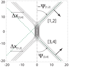
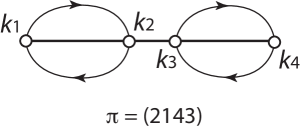
Figure 2.4: X-type soliton interaction with phase shifts $\Delta x_{[i,j]}$ and the chord diagram.

It is quite important to note that in a real physical situation, the phase shift determined by the amplitudes and slopes of solitary waves forming X-shape pattern should be of the same order of scaling as used in the derivation of the KP equation from the Euler equations. The scaling for the KP equation is given by the parameter $\epsilon\sim a_{0}/h_{0}\sim(h_{0}/\lambda_{0})^{2}\sim\tan^{2}\psi_{0}$ where $a_{0}$ is the wave amplitude, $h_{0}$ is the water depth, $\lambda_{0}$ is the wavelength and $\psi_{0}$ is the slope of the soliton. The typical value of $\epsilon$ in real physical situation ranges from $10^{-2}$ to $10^{-1}$. If we take $\epsilon\approx 10^{-2}$, then the phase shift can be at most twice the soliton wavelength. In Figure 2.4, we take $2A_{0}=\epsilon$ and $\tan^{2}\Psi_{0}=(1+2\cdot 10^{-4})\epsilon$ i.e., $\tan^{2}\Psi_{0}-A_{0}=\epsilon 10^{-4}$ in (2.8), in order to demonstrate a large phase shift ($\sim$ 4 times the the soliton wavelength). Such large phase shifts are highly atypical since a small difference of $\epsilon 10^{-4}\approx\epsilon^{3}$ between physical quantities which are of order $\epsilon$ can be easily destroyed by small external perturbations or even by the higher order effects. (If $\epsilon\approx 10^{-1}$, then we need the accuracy of order $\epsilon^{5}=10^{-4}\epsilon$). In this sense, a long stem observed in a real wave pattern cannot be due to the phase shift. In other words, the wave pattern having a long stem does not correspond to an X-soliton of the KP equation. For example, the wave pattern in Figure 2.5(a) shows an X-type interaction, while the wave pattern in Figure 2.5(b) is not of X-type, and the stem appearing in the middle of Figure 2.5(b) is an intermediate solitary wave which interact resonantly with other two solitons at the trivalent vertices. In fact, we expect the wave pattern shown in Figure 2.5(b) to be non-stationary (although records of its time evolution is not available to us). In the framework of KP theory, the wave patterns in Figures 2.5 approximate two entirely different soliton solutions of the KP equation.

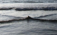
(a)               (b) 

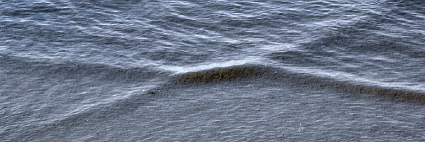
Figure 2.5: Photographs by M. J. Ablowitz (left panel) and D. E. Baldwin (right panel) [2]

Remark 2.1

From (2.8), one can see that this type of X-soliton solution exists only if $2A_{0}<\tan^{2}\Psi_{0}$. The formula (2.8) breaks down at the critical slope $\tan^{2}\Psi_{c}:=2A_{0}$, whence a new soliton solution of KP emerges at this limit. In this case, the X-vertex degenerates to a Y-vertex as the two solitons interact resonantly and generate a third soliton, called the Mach stem [18]. One can also compute the maximum amplitude occurring at the mid-point of the interaction, and it is given by [7]

$$u_{\text{max}}=\frac{4A_{0}}{1+\sqrt{\Delta_{0}}}\quad\text{with}\quad\Delta_{0}:=1-\frac{2A_{0}}{\tan^{2}\Psi_{0}}.$$

Then at the critical angle $\Psi_{c}$, the maximum amplitude can reach four times of the solitons. This interaction phenomena is referred to as the Mach reflection which has important application in the study of rogue waves. A recent study on the Mach reflection for KP solitons can be found in [16]. In particular, it was found in [13] that the line-soliton solution of type $\pi=(3142)$ can be used to describe the non-stationary wave patterns generated by the Mach reflection for the cases with $2A_{0}>\tan^{2}\Psi_{0}$, where the X-soliton becomes singular (see [18]).

A general line-soliton solution of the KP equation can be regarded as a collection of one-solitons and Y-solitons which fit together to form a web-structure with X- and Y-vertices in the interaction region as shown in Figure 2.6. An alternate combinatorial description of this solution can be obtained by gluing the local chord diagrams corresponding to those component one-solitons and Y-solitons and to form the complete chord diagram for the derangement $\pi$ associated with the general soliton solution. We will implement this technique of “gluing” of chords in the next section in order to reconstruct a KP soliton solution from a real wave pattern and will illustrate this method with explicit examples.

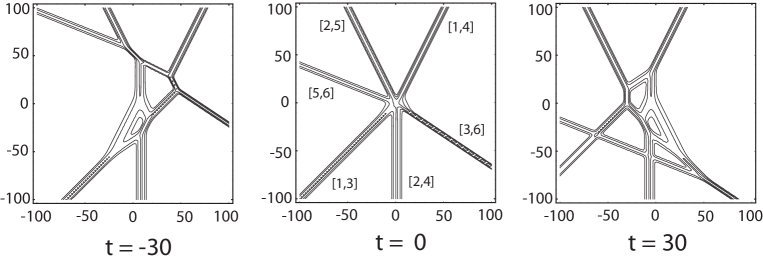
Figure 2.6: Example of web-soliton solution with $\pi=\binom{1~{}2~{}3~{}4~{}5~{}6}{4~{}5~{}1~{}2~{}6~{}3}$.

3 Inverse problem

In this section we discuss the problem of constructing an exact soliton solution of the KP equation from a given wave pattern satisfying the assumptions required to derive the KP equation. In other words, the pattern should describe interactions of small amplitude, quasi-two-dimensional waves of long wavelength traveling in one direction. Here we consider the surface wave patterns on shallow water observed in long, flat stretches of ocean beaches. Provided that the wave pattern approximates a KP soliton solution, we assume that each component wave in the pattern approximates a $[i,j]$-soliton for some index pair $i<j$. Then the construction procedure consists of the following steps:

1. Set the $xy$-coordinates, so that all solitary waves in the pattern are traveling almost in the positive $x$-direction (towards the shore).

2. Using (2.6) and (2.7), find the $k$-parameters by measuring the amplitudes and slopes of the solitary waves in the pattern.

3. Define the derangement $\pi$ and its chord-diagram from the $k$-parameters obtained in the step 2.

4. Determine the form of the totally non-negative matrix $A$ from the derangement $\pi$ using combinatorial techniques [15].

5. Using (2.5), find the matrix elements of $A$ from the minors $\Delta_{I}(A)$ by measuring the locations of the solitary waves in the pattern.

We remark that if there are resonances in the wave pattern, it is sufficient to measure the amplitudes, or slopes or locations of only a subset of the solitary wave forms in the pattern, rather than the entire set.

The wave patterns that we consider for the inverse problem are assumed to be generic in the sense that the topological structure of the pattern remains the same over a finite period of time. That is, the number of X- and Y-vertices in the pattern remains the same over a certain time period. If a generic wave pattern contains a line soliton which interacts non-resonantly with all other waves (i.e. the interactions make only X-vertices), then it can be treated as a separate $[i,j]$-soliton in the sense that its chord-diagram (see Figure 2.1) is disjoint (non-crossing) from the chord diagram of the remaining pattern. It is for this reason we only consider wave patterns where each line soliton is incident on at least one trivalent vertex. That is, each line soliton interacts resonantly with two other line solitons forming a Y-vertex.

In this note, we primarily consider wave patterns with only two trivalent vertices consisting of two Y-type (one Y-shape and other Y -shape) waves which have a common intermediate solitary wave. We distinguish the Y-type waves by marking their trivalent vertices, in particular, we assign a white vertex for the Y -shape wave, and a black vertex for the Y-shape wave. Identifying the common intermediate wave from each Y-shape wave, one can see that there are 5 distinct cases for such wave pattern as shown in Figure 3.1.

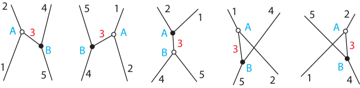
Figure 3.1: Five distinct wave patterns obtained by gluing two Y-shape waves.

The resonant vertices in each of these patterns are labeled $\mathsf{A}$ (upper vertex) and $\mathsf{B}$ (lower vertex). The solitary waves incident at the vertex $\mathsf{A}$ are numbered as 1, 2 and 3, while the solitary waves numbered as 3, 4 and 5 are incident at the vertex $\mathsf{B}$. Thus each pattern consists of two Y-type waves glued together by the common solitary wave 3 joining vertices $\mathsf{A}$ and $\mathsf{B}$. Besides serving as simple examples to illustrate our method, these patterns are observed fairly regularly in flat ocean beaches. However, such wave patterns cannot be modeled by Hirota’s 2-soliton formula which gives a stationary pattern, and contains only one free parameter determining the phase shift due to non-resonant interaction of the $X$-soliton described in Section 2.3. The exact line-soliton solutions corresponding to these resonant wave patterns are non-stationary and contain more than one free parameters (a complete classification of the line-soliton solutions corresponding to those patterns in Figure 3.1 is given in [7]).

In order to construct KP solitons from those patterns, we first identify each solitary wave with an $[i,j]$-soliton for some parameters $k_{i}<k_{j}$. Let us assign $\{k_{a},k_{b},k_{c}\}$ at the vertex $\mathsf{A}$, and $\{k_{a^{\prime}},k_{b^{\prime}},k_{c^{\prime}}\}$ at the vertex $\mathsf{B}$. Thus each one-soliton can be parametrized as follows:

Soliton 1	Soliton 2	Soliton 3	Soliton 4	Soliton 5
$\{k_{a},k_{b}\}$	$\{k_{a},k_{c}\}$	$\{k_{b},k_{c}\},\{k_{b^{\prime}},k_{c^{\prime}}\}$	$\{k_{a^{\prime}},k_{b^{\prime}}\}$	$\{k_{a^{\prime}},k_{c^{\prime}}\}$

Note that there are two parametrizations (with respect to the two vertices A and B) for the intermediate soliton 3 which is common to the Y-solitons. Let $\tan\Psi_{i},\,i=1,2,\ldots,5$ denote the slope of each one-soliton. In particular, the slope of soliton 3 is given as $\tan\Psi_{3}=k_{b}+k_{c}=k_{b^{\prime}}+k_{c^{\prime}}$. Then the $k$-values can be solved uniquely from the slope measurements at the vertices $\mathsf{A}$ and $\mathsf{B}$ for each Y-soliton as given by (2.7), i.e.

$$\left\{\begin{array}[]{lll}k_{a}={\textstyle\frac{1}{2}}(\tan\Psi_{1}+\tan\Psi_{2}-\tan\Psi_{3})\,,\\[2.15277pt] k_{b}=\tan\Psi_{1}-k_{a}\,,\quad k_{c}=\tan\Psi_{2}-k_{a},\end{array}\right.$$ (3.1c)

$$\left\{\begin{array}[]{lll}k_{a^{\prime}}={\textstyle\frac{1}{2}}(\tan\Psi_{4}+\tan\Psi_{5}-\tan\Psi_{3})\,,\\[2.15277pt] k_{b^{\prime}}=\tan\Psi_{4}-k_{a^{\prime}}\,,\quad k_{c^{\prime}}=\tan\Psi_{5}-k_{a^{\prime}}\end{array}\right.$$ (3.1f)

Without loss of generality, the two sets of $k$-parameters for soliton 3 can be ordered as $k_{b}<k_{c}$ and $k_{b^{\prime}}<k_{c^{\prime}}$. If the given wave pattern is an exact KP soliton, then one should have $k_{b}=k_{b^{\prime}}$ and $k_{c}=k_{c^{\prime}}$. But from equations (3.1c) and (3.1f) we have

$$k_{b}-k_{b^{\prime}}=-(k_{c}-k_{c^{\prime}})={\textstyle\frac{1}{2}}[(\tan\Psi_{1}-\tan\Psi_{2})-(\tan\Psi_{4}-\tan\Psi_{5})].$$

This has a non-zero value which measures the deviation from the KP soliton and is also due to the error in the measurement. To approximate a real wave pattern by a KP soliton, it is reasonable to prescribe the $k$-parameters of soliton 3 by taking the average of the two sets of $k$-values. Therefore, we define the $k$-parameters of soliton 3 as

$$\tilde{k}_{b}={\textstyle\frac{1}{2}}(k_{b}+k_{b^{\prime}}),\qquad\quad\tilde{k}_{c}={\textstyle\frac{1}{2}}(k_{c}+k_{c^{\prime}})\,,$$

which preserves the slope of soliton 3, i.e., $\tan\Psi_{3}=\tilde{k}_{b}+\tilde{k}_{c}$, and leads to the following re-parametrization of the line solitons:

Soliton 1	Soliton 2	Soliton 3	Soliton 4	Soliton 5
$\{k_{a},\tilde{k}_{b}\}$	$\{k_{a},\tilde{k}_{c}\}$	$\{\tilde{k}_{b},\tilde{k}_{c}\}$	$\{k_{a^{\prime}},\tilde{k}_{b}\}$	$\{k_{a^{\prime}},\tilde{k}_{c}\}$

We remark here that the conditions $k_{b}=k_{b^{\prime}}$ and $k_{c}=k_{c^{\prime}}$, are consequences of the fact that the amplitudes $A_{[b,c]}=A_{[b^{\prime},c^{\prime}]}$ in the exact KP theory. In fact, from the amplitude formula in (2.6), we have

$$k_{b}-k_{b^{\prime}}=-(k_{c}-k_{c^{\prime}})=\frac{1}{2}\left(\sqrt{2A_{[b,c]}}-\sqrt{2A_{[b^{\prime},c^{\prime}]}}\right)\,,$$

which vanishes when $A_{[b,c]}=A_{[b^{\prime},c^{\prime}]}$. One should however note that the amplitude along a solitary wave in the pattern may not be uniform giving rise to different measurements at the vertices A and B. Moreover, the amplitude formula $A_{[i,j]}={\textstyle\frac{1}{2}}(k_{i}-k_{j})^{2}$ is only correct up to first order, and one needs higher order corrections to obtain the corresponding KP amplitude [16] (see also Lecture 1 in [12]). On the other hand, the slope of each solitary wave in the observation is the same as that used in the KP equation. For this reason, we determine the $k$-parameters from the slope measurements only.

In what follows, we provide a step by step algorithm to reconstruct the exact KP soliton solution from a given wave pattern with two trivalent resonant vertices.

3.1 Algorithm for the inverse problem

For specificity, we use a real example of the wave pattern in Figure 3.2 which corresponds to the first pattern in Figure 3.1.

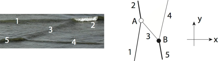
Figure 3.2: A real example of the wave pattern corresponding to the first pattern in Figure 3.1. Photograph of the wave pattern taken by D. E. Baldwin [2]

Step 1: Finding the $k$-parameters

We first set the $xy$-coordinates, so that the wave is propagating along almost $x$-direction. We choose the origin as the vertex $\mathsf{A}$ in Figure 3.2. Then we trace the wave crests as a graph, and measure the angles of all the line solitons with respect to the positive $y$-axis. For this example, we estimate the angles for the line solitons to be

$$\Psi_{1}=-15^{\circ},\quad\Psi_{2}=3^{\circ},\quad\Psi_{3}=25^{\circ},\quad\Psi_{4}=-13^{\circ},\quad\Psi_{5}=~{}5^{\circ}.$$

Next from (3.1c) and (3.1f), one obtains $k_{a}=-0.341,k_{b}=0.073$ and $k_{c}=0.393$ at the vertex $\mathsf{A}$, and $k_{a^{\prime}}=-0.305,k_{b^{\prime}}=0.074$ and $k_{c^{\prime}}=0.392$ at the vertex $\mathsf{B}$. After averaging to get $\tilde{k}_{b},\tilde{k}_{c}$ and then arranging the $k$-parameters in increasing order gives

$$(k_{a},k_{a^{\prime}},\tilde{k}_{b},\tilde{k}_{c})=(k_{1},k_{2},k_{3},k_{4})=(-0.341,-0.305,0.0735,0.3925)\,.$$

Note that the slope data at the resonant vertices is sufficient to obtain the $k$-parameters, the amplitude data for the solitons, which is difficult to measure from a photograph, is not necessary in this case. Note that the amplitude of each one-soliton can be calculated from the $k$-values using (2.6). Here we see that the soliton 2 has the maximum amplitude, $A_{[1,4]}={\textstyle\frac{1}{2}}(k_{4}-k_{1})^{2}=0.269$, and the soliton 3 has the maximum slope, $\tan\Psi_{[3,4]}=k_{3}+k_{4}=0.466$. These are rather large values for the KP approximation, and we may need higher order corrections to obtain a better result (see Lecture 1 in [12]).

From this set of $k$-parameters, the procedure to find the derangement $\pi$ for the data may be illustrated as a process of gluing the chord diagrams of the two Y-solitons with vertices $\mathsf{A}$ and $\mathsf{B}$ through the common chord as illustrated in Figure 3.3. At the vertex $\mathsf{A}$, one has a Y -soliton of the type formed by line solitons labeled 1,2 and 3, and the corresponding chord diagram is indicated by the top diagram in the middle of Figure 3.3. The dots in this diagram denote the $k$-parameters $k_{a}<k_{b}<k_{c}$. Similarly, the bottom chord diagram corresponds to the Y-soliton at the vertex $\mathsf{B}$ formed by solitons 3,4 and 5 with the dots marking the $k$-parameters $k_{a^{\prime}}<k_{b^{\prime}}<k_{c^{\prime}}$. Notice that the common chord (labeled 3) in these two diagrams correspond to soliton 3 joining the vertices $\mathsf{A}$ and $\mathsf{B}$. We then superpose the top and bottom diagrams and ignore the common chord for the intermediate soliton 3 and recover the complete chord diagram of the asymptotic solitons shown by the rightmost diagram in Figure 3.3. In this diagram the $k$-parameters are marked (by the 4 dots) as $k_{a}=k_{1},k_{a^{\prime}}=k_{2}$ and the average values $\tilde{k}_{b}=k_{3},\tilde{k}_{c}=k_{4}$ with $k_{1}<k_{2}<k_{3}<k_{4}$. This diagram corresponds to the derangement $\pi=\left(\begin{smallmatrix}1&2&3&4\\ 4&3&1&2\end{smallmatrix}\right)$, or simply as $\pi=(4312)$ which is the one-line notation of permutation. The top chords in this diagram are associated to the asymptotic solitons 2 and 4 for $y\gg 0$ which are identified as $[1,4]$- and $[2,3]$-soliton. Similarly, the bottom chords in this diagram are associated to the $[1,3]$- and $[2,4]$- asymptotic line solitons for $y\ll 0$. This is summarized in Figure 3.3.

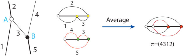
Figure 3.3: Chord gluing algorithm for the wave pattern in Figure 3.2

Step 2: Finding the form of the $A$-matrix

Recall that in order to construct the $\tau$-function in (2.2) for the soliton solutions, one needs the $N\times M$ totally nonnegative matrix $A$ in addition to the $k$-parameters. The $A$-matrix can derived from the derangement $\pi$ obtained in Step 1 by employing combinatorial methods based on Deodhar decomposition of Grassmann varieties. This has been developed in a recent paper by Kodama and Williams [15], we refer the interested readers to that article and omit the details in this short note. Alternatively, the interested reader may also consult the work of Chakravarty and Kodama [5, 7] where in particular, the $A$-matrices for those patterns in Figure 3.1 were explicitly given in reduced row echelon form for the corresponding derangements $\pi$. For the current example with $\pi=(4312)$, the $A$-matrix is given by either

$$A=\begin{pmatrix}p_{3}p_{4}&p_{4}&0&-1\\ 0&p_{1}&1&0\end{pmatrix}\quad\text{or}\quad\begin{pmatrix}1&0&-b&-c\\ 0&1&a&0\end{pmatrix},$$

with three real parameters $\{p_{1},p_{3},p_{4}\}$ or $\{a,b,c\}$. The second matrix (given in [7]) is the reduced row echelon form of the first one. Note that $A$ is a totally nonnegative matrix, i.e., $\Delta_{I}(A)\geq 0$ for all $I\in\binom{[M]}{N}$, if all $p_{1},p_{3},p_{4}>0$ (or all $a,b,c>0$). In this case, the corresponding exact soliton solution of KP is non-singular for all $x,y$ and $t$. We also remark that the $\tau$-function generated by the matrix $A$ contains five exponential terms, i.e.

$$\tau=\mathop{\textstyle\sum}\limits_{1\leq i<j\leq 4}\Delta_{i,j}(A)E_{i,j}\qquad\text{with}\quad\Delta_{i,j}(A)\neq 0~{}~{}\text{except}~{}~{}\Delta_{1,4}(A)=0.$$

One should compare this with the case of X-soliton where the $\tau$-function has four exponential terms. Notice that if $p_{4}=0$ (or $b=0$) with keeping $p_{3}p_{4}=a$ and $p_{1}=c$, then the corresponding X-soliton consists of $[1,4]$- and $[2,3]$-solitons with the phase shift, i.e. the X-soliton is of the type $\pi=(4321)$.

Step 3: Determining the values of the $A$-matrix

The last step is to explicitly find the entries of the $A$-matrix. This is accomplished by evaluating the $p$-parameters from the given wave pattern.

Figure 3.4 shows the wave pattern of our example with all the $[i,j]$ asymptotic solitons labeled. The index set $I=\{i,j\},\,i<j$ indicates each region in the $xy$-plane where the exponential $E_{I}$ is dominant. The corresponding minor $\Delta_{I}(A)$ of the matrix $A$ with column set $I$ is given in terms of the $p$-parameters. Recall from the previous section that the equation of the line corresponding to the $[i,j]$-soliton is given by $\Theta_{[i,j]}=0$ for a fixed value of $t$, where $\Theta_{[i,j]}$ is given by (2.5). Notice that the expression for $\Theta_{[i,j]}$ contains the constant $x_{[i,j]}$ which involves the ratios of the minors $\Delta_{I}(A)$ and $\Delta_{J}(A)$ where $I$ and $J$ label the adjacent regions in the $xy$-plane whose common boundary is the line corresponding to the $[i,j]$-soliton.

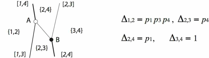
Figure 3.4: Dominant exponentials and the minors of the matrix $A$ for the wave pattern in Figure 3.2

We pick a point $(x_{0},y_{0})$ on the line corresponding to the $[2,4]$-soliton in Figure 3.4. Setting the time $t=0$, we have the equation of this line,

$$x+(k_{2}+k_{4})y+\frac{1}{k_{2}-k_{4}}\ln\frac{\Delta_{2,3}(A)(k_{3}-k_{2})}{\Delta_{3,4}(A)(k_{4}-k_{3})}=0\,.$$

Using the facts that $\Delta_{3,4}(A)=1$ and the point $(x_{0},y_{0})$ is on the line, one obtains

$$\Delta_{2,3}(A)=p_{4}=\frac{k_{4}-k_{3}}{k_{3}-k_{2}}\exp\left((k_{4}-k_{2})x_{0}+(k_{4}^{2}-k_{2}^{2})y_{0}\right)\,.$$

Similarly, selecting a point $(x_{0},y_{0})$ on line corresponding to the $[2,3]$-soliton, yields

$$\Delta_{2,4}(A)=p_{1}=\frac{k_{4}-k_{3}}{k_{4}-k_{2}}\exp\left((k_{3}-k_{2})x_{0}+(k_{3}^{2}-k_{2}^{2})y_{0}\right)\,,$$

and finally, by choosing a point on either the $[1,4]$- or the $[1,3]$-line, one can get $\Delta_{1,2}(A)$, which in turn, yields $p_{3}$. In this way, we can evaluate the $p$-parameters (hence the $A$-matrix) from the graph corresponding to a photograph of the wave pattern after we have identified all the $[i,j]$-solitons in the pattern.

For this example, we chose the origin as the vertex $\mathsf{A}$ common to lines corresponding to the $[1,3]$- and $[1,4]$-solitons, and estimate the location of the vertex $\mathsf{B}$ as $(50,-107.2)$ which lie on the $[2,3]$- and $[2,4]$-soliton lines. Taking $(x_{0},y_{0})$ as those points, we obtain the values $p_{1}=9.1\times 10^{11},\,p_{3}=1.1\times 10^{-11},\,p_{4}=16.9\times 10^{11}$ which gives the exact $A$-matrix in Step 2. From this $A$-matrix and the $k$-parameters already found in Step 1, one can now construct the $\tau$-function and the KP soliton solution using (2.1). Plots of the exact solution, $u=2(\ln\tau)_{xx}$, which approximates the snapshot of the original wave pattern (Figure 3.2), are shown in Figure 3.5. The middle plot at $t=0$ corresponds to the photograph of the wave pattern in Figure 3.2, the left and right plots are for $t<0$ and $t>0$, respectively. Notice that the wave pattern is not stationary, and the stem (soliton 3) is getting shorter which means it is a an intermediate soliton rather than a stationary phase shift.

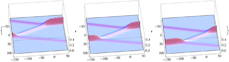
Figure 3.5: Evolution of the KP soliton constructed from the wave pattern in Figure 3.2.

4 Examples

Here we present a few more examples to illustrate our method. In these examples we consider a succession of photographs of an evolving wave pattern and compare the dynamics with the time evolution of the exact solution reconstructed by the algorithm described in Section 3.1.

4.1 Example 1: An Estonian beach

The top panel in Figure 4.1 shows a snapshot of a wave pattern observed on a beach of Lake Peipsi, Estonia. This photograph is part of a video footage capturing the dynamics of the wave pattern over a period of time. This corresponds to the wave pattern of the fourth case in Figure 3.1 with two Y-vertices and an X-vertex. We then apply our inverse problem algorithm to this snapshot, which is chosen to be $t=0$, to construct the exact solution $u(x,y,0)$, then compare $u(x,y,t)$ for $t\neq 0$ with other snapshots taken from the video footage. The middle picture of the top panel in Figure 4.1 shows the graph traced from the wave crests in the pattern. The solitary waveforms in the pattern are not straight lines, we first locate the vertices and join them to obtain the lines marked 2,3 and 4. The lines 1 and 5 are traced by using the slopes computed at each of their respective vertices. From the trace the angles of the line solitons are estimated to be $\Psi_{1}=14^{\circ},\,\Psi_{2}=37^{\circ},\,\Psi_{3}=0^{\circ},\,\Psi_{4}=-42^{\circ},\Psi_{5}=-20^{\circ}$. Following Step 1 in Section 3.1, we obtain the $k$-parameters as $(k_{1},k_{2},k_{3},k_{4})=(-0.632,-0.268,0.268,0.517)$. Then we have the derangement $\pi=(2413)$ as shown in the top right panel of Figure 4.1. Here solitons 2 and 5 correspond to the $[3,4]$- and $[1,3]$-solitons respectively, for $y\ll 0$, whereas solitons 1 and 4 correspond to $[2,4]$- and $[1,2]$-solitons for $y\gg 0$. Finally, we construct the exact solution following the prescription in Steps 2 and 3. The bottom two panels of Figure 4.1 exhibit the comparison between the time evolutions of the exact solution and the actual wave pattern. The last snapshot in the middle panel is the snapshot corresponding to $t=0$ from which the exact KP solution was constructed, the previous snapshots in the middle panel correspond to $t<0$. Also note that the leftmost snapshot corresponds to the wave pattern of the third case in Figure 3.1 indicating that the evolving solution can coincide with more than one configuration shown in Figure 3.1.

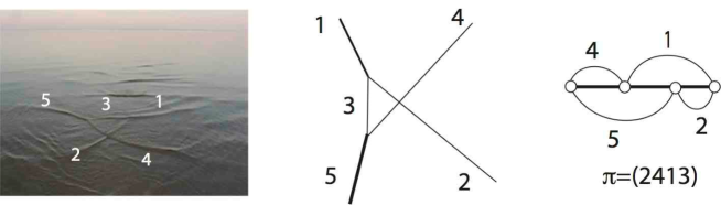
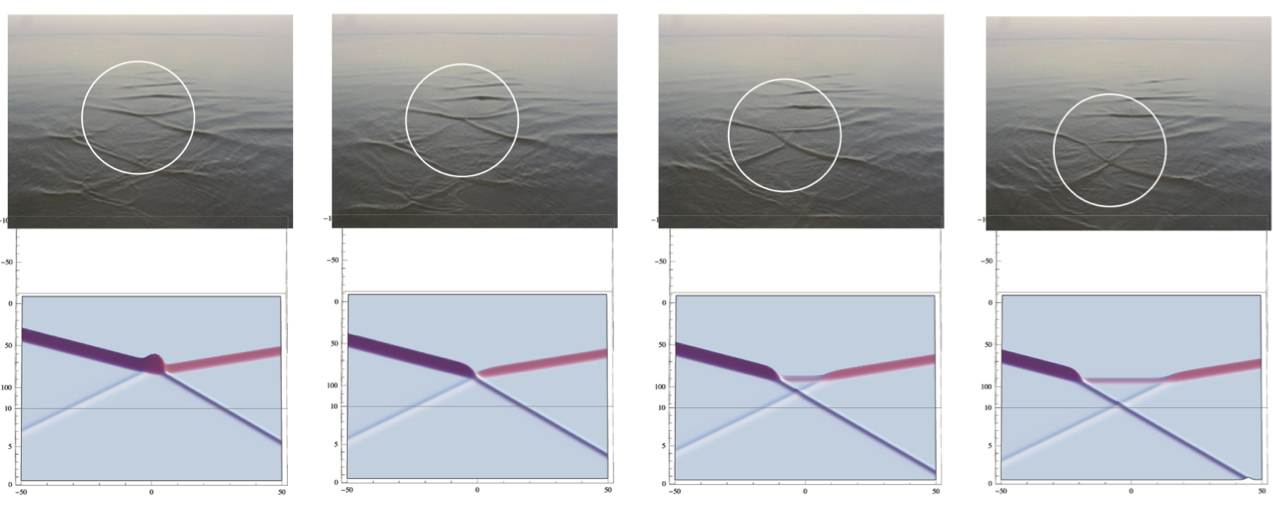
Figure 4.1: Waves in Lake Peipsi, Estonia. Snapshots from a video courtesy Ira Didenkulova.

4.2 Example 2: An Mexican beach

Our next example is from Figure 1.1 in Section 1 showing a wave pattern with three line solitons for $y\gg 0$ and two line solitons for $y\ll 0$. The left photograph in the figure was used to reconstruct the exact solution at $t=0$, the right photograph is of the same wave pattern taken at some $t>0$. Without giving the details we simply point out that in this case our algorithm identifies the solitons (from right to left) $[1,2]$, $[2,4]$ and $[4,5]$ for $y\gg 0$, and solitons $[1,3]$ and $[3,5]$ for $y\ll 0$, from which we have the derangement $\pi=(24153)$. Let us describe the evolution of the exact solution in Figure 4.2 in more details. There are several things to notice here. This solution has three Y-vertices and one X-vertex (these are more clear in the second and third frames). The solitons $[2,4]$ and $[4,5]$ interact at the rightmost ($y>0$) Y-vertex to form a large amplitude stem $[2,5]$-soliton which is visible in both photographs in Figure 1.1 but more pronounced in the right photograph. This clearly suggests that the $[2,5]$-soliton is not a phase shift since it is a non-stationary stem arising from a resonant interaction of the solitons $[2,4]$ and $[4,5]$ from the right ($y\gg 0$).

This $[2,5]$-soliton interacts resonantly with the $[3,5]$-soliton coming from the left ($y\ll 0$) at the second Y-vertex to form a small amplitude $[2,3]$-soliton which is barely discernible in the first frame as well as the wave pattern photograph in Figure 1.1. But as the pattern evolves the $[2,3]$-soliton is clearly visible in the second, third and fourth frames in Figure 4.2 as well as the right photograph of the wave pattern in Figure 1.1 taken at $t>0$. Again, this clearly shows that the length of the $[2,3]$-soliton grows with time. The $[2,3]$-soliton intersects with the $[1,2]$-soliton on the right ($y\gg 0$) and the large amplitude asymptotic $[1,3]$-soliton on the left ($y\ll 0$) at the third Y-junction (seen on the left, in the second and third frames) to form a resonant triplet.

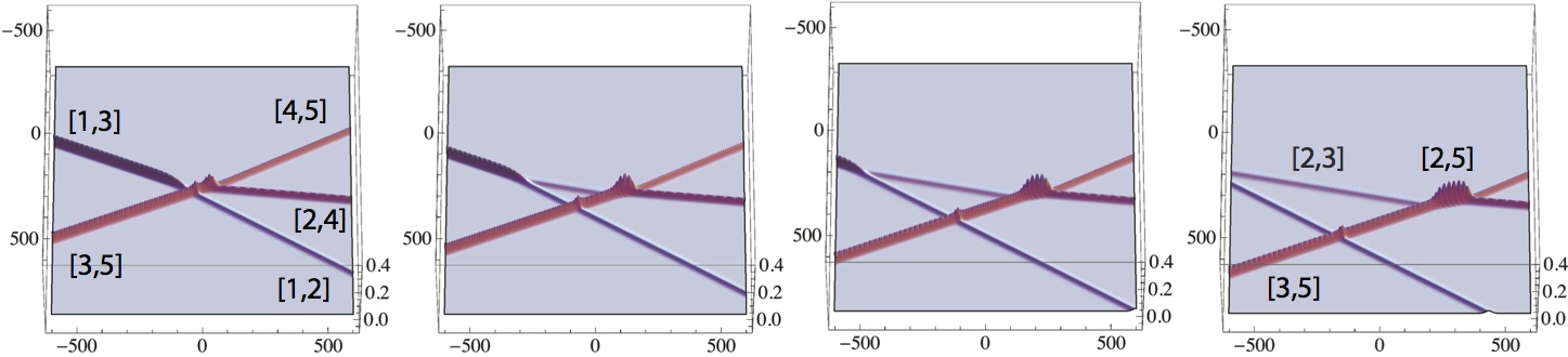
Figure 4.2: Evolution of the KP soliton constructed from the wave pattern in Figure 1.1

5 Conclusion

In this note we described an explicit algorithm to construct an exact solution of the KP equation approximating a given pattern of small amplitude, long wavelength and primarily unidirectional shallow water waves. This can be regarded as an “inverse problem” in the sense that by measuring some metric data such as the angles and locations of the solitary waves in the given pattern with respect to a fixed reference frame, it is possible to determine the data necessary to construct the $\tau$-function associated with a KP line-soliton solution. We have illustrated our method by applying it to photographs and videos of real wave patterns. The constructed exact solutions compare fairly well with the snapshots (at a fixed $t$) but more importantly we have shown that their time evolution is also in good agreement with the dynamics of these non-stationary patterns. These exact solutions of the KP equation found in Sections 3 and 4 were derived and classified in previous works by the authors, and they cannot be obtained from a simple Hirota $N$-soliton formula.

An important feature of this algorithm is that one can directly read off the parameters for the exact soliton solution from the wave pattern data without resorting to any ad hoc techniques to “guess” the soliton parameters from the wave pattern. One could also incorporate the measurement of amplitudes of the wave forms in the algorithm although the measurement of the slopes are generally more accurate than that of the amplitudes of the wave forms in the pattern. The possible inaccuracies in amplitude measurement are due to, for example, the breaking of the waves and the higher order corrections to the leading order KP equation. Moreover, it is difficult (if not impossible) to measure the amplitudes if one were to use a photograph (or a video) of the wave pattern. The slopes of the line solitons should be measured at a vertex (intersection points of the interacting solitons), since the solitary wave form may not be exactly a straight-line e.g., due to non-constant depth of water on a beach. Our algorithm can be extended in principle to a wave pattern with arbitrary number of solitary waves for $y\gg 0$ and $y\ll 0$ although such patterns may be unstable and break up shortly after it is formed due to external perturbations.

References

- [1] M. J. Ablowitz and D. E. Baldwin, Nonlinear shallow ocean-wave soliton interactions on flat beaches, Phys. Rev. E, 86 (2012) 036305 (5pp).
- [2] M. J. Ablowitz and D. E. Baldwin, Photographs and videos at http://www.markablowitz.com/line-solitons and http://www.douglasbaldwin.com/nl-waves.html.
- [3] G. Biondini and S. Chakravarty, Soliton solutions of the Kadomtsev-Petviashvili II equation, J. Math. Phys., 47 (2006) 033514.
- [4] G. Biondini and Y. Kodama, On a family of solutions of the Kadomtsev-Petviashvili equation which also satisfy the Toda lattice hierarchy, J. Phys. A: Math. Gen. 36 (2003) 10519-10536.
- [5] S. Chakravarty and Y. Kodama, Classification of the line-solitons of KPII, J. Phys. A: Math. Theor., 41 (2008) 275209 (33pp).
- [6] S. Chakravarty and Y. Kodama, A generating function for the -soliton solutions of the Kadomtsev-Petviashvili II equation, Contemp. Math., 471 (2008) 47-67.
- [7] S. Chakravarty and Y. Kodama, Soliton Solutions of the KP Equation and Application to Shallow Water Waves, Stud. Appl. Math., 123 (2009) 83–151.
- [8] R Hirota, The Direct Method in Soliton Theory (Cambridge University Press, Cambridge, 2004).
- [9] B. B. Kadomtsev and V. I. Petviashvili, On the stability of solitary waves in weakly dispersive media, Sov. Phys. - Dokl. 15 (1970) 539-541.
- [10] Y. Kodama, Young diagrams and N-soliton solutions of the KP equation, J. Phys. A: Math. Gen. 37 (2004) 11169-90.
- [11] Y. Kodama, KP solitons in shallow water, J. Phys. A: Math. Theor., 43 (2010) 434004 (54pp).
- [12] Y. Kodama, Lectures delivered at the NSF/CBMS Regional Conference in the Mathematical Sciences “Solitons in Two-Dimensional Water Waves and Applications to Tsunami”, UTPA, May 20–24, 2013 (Lecture slides are available at http://faculty.utpa.edu/kmaruno/nsfcbms-tsunami.html).
- [13] Y. Kodama, M. Oikawa and H. Tsuji, Soliton solutions of the KP equation with V-shape initial waves, J. Phys. A:Math. Theor., 42 (2009) 312001 (9pp).
- [14] Y. Kodama and L. Williams, KP solitons and total positivity for the Grassmannian, (arXiv:1106.0023).
- [15] Y. Kodama and L. Williams, The Deodhar decomposition of the Grassmannian and the regularity of KP solitons, Adv. Math., 244 (2013) 979-1032.
- [16] W. Li, H. Yeh and Y. Kodama, On the Mach reflection of a solitary wave: revisited, J. Fluid Mech. 672 (2011) 326-357.
- [17] J. W. Miles, Obliquely interacting solitary waves, J. Fluid Mech., 79 (1977) 157-169.
- [18] J. W. Miles, Resonantly interacting solitary waves, J. Fluid Mech., 79 (1977) 171-179.
- [19] A. C. Newell and L. G. Redekopp, Breakdown of Zakharov-Shabat theory and soliton creation, Phys. Rev. Lett. 38 (1977) 377-380.
- [20] P. Peterson and E van Groesen, A direct and inverse problem for wave crests modeled by intersections of two solitons, Physica D 141 (2000) 316-332.
- [21] P. Peterson, Reconstruction of multi-soliton interactions using crest data for (2+1)-dimensional KdV type equations, Physica D 171 (2002) 221-235.
- [22] T. Soomere and J. Engelbrecht, Weakly two-dimensional interaction of solitons in shallow water, Eur. J. Mech. B Fluids, 25 (2006) 636-648.
- [23] H. Yeh, Laboratory Realization of Kodama’s KP-Solitons, Lecture delivered at the NSF/CBMS Regional Conference in the Mathematical Sciences “Solitons in Two-Dimensional Water Waves and Applications to Tsunami”, UTPA, May 20–24, 2013 (Lecture slides are available at http://faculty.utpa.edu/kmaruno/nsfcbms-tsunami.html).