UNDERSTANDING THE UNUSUAL X-RAY EMISSION PROPERTIES OF THE MASSIVE, CLOSE BINARY WR 20A: A HIGH ENERGY WINDOW INTO THE STELLAR WIND INITIATION REGION

Abstract

The problem of explaining the X-ray emission properties of the massive, close binary WR 20a is discussed. Located near the cluster core of Westerlund 2, WR 20a is composed of two nearly identical Wolf- Rayet stars of 82 and 83 solar masses orbiting with a period of only 3.7 days. Although Chandra observations were taken during the secondary optical eclipse, the X-ray light curve shows no signs of a flux decrement. In fact, WR 20a appears slightly more X-ray luminous and softer during the optical eclipse, opposite to what has been observed in other binary systems. To aid in our interpretation of the data, we compare with the results of hydrodynamical simulations using the adaptive mesh refinement code Mezcal that includes radiative cooling and a radiative acceleration force term. It is shown that the X-ray emission can be successfully explained in models where the wind-wind collision interface in this system occurs while the outflowing material is still being accelerated. Consequently, WR 20a serves as a critical test-case for how radiatively-driven stellar winds initiate and interact. Our models not only procure a robust description of current Chandra data, which cover the orbital phases between 0.3 to 0.6, but provide detailed predictions over the entire orbit.

1. Introduction

Among the most massive stars, which tend also to be the hottest and most luminous, the emanating stellar winds can be very strong, with important consequences for both the star’s own evolution as well as for the character of the emitting radiation. There is extensive evidence that hot-star winds are not the smooth, steady outflows idealized in the simple CAK theory (Castor et al., 1975) but rather have extensive substructure (Lucy & White, 1980; Owocki, 2011). Massive O-type and Wolf-Rayet (WR) stars commonly show soft X-ray emission (Nazé, 2009; Skinner et al., 2012) and sometimes also non-thermal radio emission (Abbott et al., 1986; Cappa et al., 2004; Montes et al., 2009), both of which are thought to originate from embedded wind shocks. In binary systems, the kinetic energy of the winds can be efficiently reconverted into radiation by shocks which form when the stellar winds collide (Usov, 1992). The resultant hard ($\mathrel{\hbox to0.0pt{\lower 4.0pt\hbox{\hskip 1.0pt$\sim$}\hss}\raise 1.0pt\hbox{$>$}}2$ keV) X-ray component (e.g., Stevens et al., 1992) usually dominates the total X-ray luminosity, greatly exceeding the empirical relation log($L_{x}/L_{\rm bol})\sim-6.9$ found for single hot massive stars (Chlebowski et al., 1989; Sana et al., 2006). The study of the X-ray emission from colliding binaries represents an indirect way of studying the properties of the stellar wind itself (e.g., Pittard & Corcoran, 2002). The hardness of the emission is related to the shock temperature which in turns depends on the pre-shock velocity of the wind. The X-ray brightness, on the other hand, is sensitive to the pre-shock density of the wind, and hence on the mass loss rate.

The theory for winds emanating from hot stars is mature enough that it is now finding application in many more complex circumstances. One example is colliding winds of close, massive star binaries. In several cases these involve massive O-type and WR members with separations of only a few stellar radii. In these systems, a wind-wind interface can occur while material is still being accelerated (Antokhin et al., 2004; Pittard, 2009). This suggests that observations of very close massive binaries could help understand how massive stars drive winds. However, most of the X-ray studies in massive binaries have been performed for systems with orbital periods of months to years (e.g., WR 140, Pollock et al., 2005), and the relationship between the X-ray emission and the wind properties in short-period systems has been difficult to determine because of a variety of added complications such as wind absorption and strong radiative interactions.

WR 20a is a close massive binary system well-suited to study how radiatively-driven stellar winds initiate and interact. This eclipsing binary system is composed of two almost identical stars (82+83 $M_{\odot}$; WN6ha+WN6ha) in a circular orbital with a period of $\sim 3.7$ days (Bonanos et al., 2004; Rauw et al., 2005). X-ray emission has been detected for this system (Nazé et al., 2008) with a $L_{x}/L_{\rm bol}$ ratio greatly exceeding that observed for single WN stars (Skinner et al., 2012). What is more, the X-ray spectrum shows evidence of a hot component around 1.3-2.0 keV, supporting the idea that the X-ray emission arises from the wind-wind interaction region.

An intriguing characteristic of the X-ray lightcurve resulting from WR 20a is the lack of observed eclipses at both soft and hard X-ray energies, which are, however, evident in the optical lightcurve. Interestingly, the X-ray emission shows an increase in brightness, which is slightly more pronounced at softer energies (10-20%), when the wind-wind interaction region is seen face-on. As a result, WR 20a appears to be brighter and somewhat softer during the secondary optical eclipse (Nazé et al., 2008). These features are very different from the X-ray lightcurves that have been observed and predicted in other systems (e.g. Pittard & Parkin, 2010), where a clear X-ray luminosity decrement is seen when the wind-wind interaction region gets occulted by the stars. One possible explanation for this unique behavior could be the orbital modulation of the absorbing wind column density, although its exact temporal dependence will be determined by the structure of the flow near the complex wind-wind interaction region.

In this paper we present two-dimensional, axisymmetric hydrodynamical simulations of the wind-wind interaction region in WR 20a and test two possible scenarios: one in which the emanating winds are assumed to have achieved their terminal velocities before interacting and another one in which the winds are still accelerating. The results of the simulations are then used to compute the X-ray emission, which are in turn compared with Chandra observations in order to help answer key remaining questions about the size and structure of the shocked and unshocked regions. Our accelerating wind model for the close interacting binary WR 20a not only provides an accurate description of current X-ray observations, which cover the orbital phases between 0.3 to 0.6, but also give detailed predictions of the expected lightcurve over the entire orbital period.

2. Modeling Wind-Wind Interactions in WR20A

Table 1Properties of WR20A as derived by 1: Bonanos et al. (2004), 2: Rauw et al. (2005), and 3: Nazé et al. (2008)

Parameter	Value	Reference
Spectral Type	WN6ha+WN6ha	1
$M$ (M⊙)	82.7 $\pm$5.5 + 81.9$\pm$5.5	1
$R_{\star}$ (R⊙)	19.3$\pm$0.5	1
$T_{\rm eff}$ (K)	43 000$\pm$2000	1
$\dot{M}$ (M⊙ yr-1)	8.5$\times\,10^{-6}$	1
$v_{\infty}$ (km s-1)	2800	1
$L_{\rm bol}$ ($L_{\odot}$)	1.91$\times 10^{6}(d/8~{}{\rm kpc})^{2}$	3
$L_{X}$ (erg s-1)	5.17$\times 10^{33}(d/8~{}{\rm kpc})^{2}$	3
$P$ (days)	3.686$\pm$0.01	2
$a$ (R⊙)	53.0$\pm$0.7	2
$i$	74∘.5$\pm$2∘.0	2
$d$ (kpc)	2-8	2

2.1. Hydrodynamical Models

The modeling of stellar wind interactions in massive binaries is challenging because the geometry of the interacting region is highly dependent on the ratio of the momentum of the emanating winds and the eccentricity of the orbit (e.g. Parkin et al., 2009; Okazaki et al., 2008; Corcoran et al., 2011, 2010; Parkin & Gosset, 2011). The high degree of symmetry in WR 20a, which is composed of two almost identical stars in a near circular orbit, allows for major simplifications to be made in both the hydrodynamical formalism and the modeling of the observed radiation (see Table 1).

To study the properties of the resultant X-ray lightcurves, we carried out two dimensional simulations of the wind interacting region using the hydrodynamics code Mezcal (De Colle & Raga, 2006; De Colle et al., 2008, 2012) including radiative cooling and a simplified radiative acceleration force term. We solve the following set of equations:

$$\frac{\partial\rho}{\partial t}+\nabla\cdot(\rho\vec{v})=0\;,$$

$$\frac{\partial\rho\vec{v}}{\partial t}+\nabla\cdot(\rho\vec{v}\vec{v}+p\mathbb{I})=f\;,$$ (1)

$$\frac{\partial e}{\partial t}+\nabla\cdot(e+p)\vec{v}=\rho\vec{f}\cdot\vec{v}-n^{2}\Lambda(T)\;,$$ (2)

where $\rho$ is the mass density, $\vec{v}$ is the velocity vector, $p$ is the thermal total pressure, $\mathbb{I}$ is the identity matrix, $e$ is the total energy defined as $e=\frac{1}{\gamma-1}p_{\rm gas}+\frac{1}{2}\rho v^{2}$ (being $\gamma=5/3$ the adiabatic index), and $\Lambda(T)$ is the coronal ionization equilibrium cooling function (Dalgarno & McCray, 1972) adapted to the abundance ratios of WN6ha stars (Antokhin et al., 2004).

In the acceleration region, the wind density is given by

$$\rho_{\rm w}(r)={\dot{M}\over 4\pi r^{2}v(r)},$$ (3)

while the wind velocity law is characterized here using a phenomenological $\beta$-law form:

$$v(r)=v_{0}+\left(v_{\infty}-v_{0}\right)\left(1-{R_{\ast}\over r}\right)^{\beta},$$ (4)

where $R_{\ast}$ is the stellar radius, $\beta$ is the velocity exponent, and $v_{0}$ is the velocity at the stellar surface, here taken for numerical convenience to be $v_{\infty}/10$.

The density and velocity radial profiles described above are introduced in the simulation by adding a force term $f$ to the momentum equation:

$$f=\frac{\dot{M}R_{\ast}\beta}{4\pi r^{4}}\left(v_{\infty}-v_{0}\right)\left(1-\frac{R_{\ast}}{r}\right)^{\beta-1}$$ (5)

In our simulations, we use a uniform grid of axial/radial size of $2\times 10^{13}$ cm, with $640$ cells along both axis, corresponding to a resolution of $\approx 3\times 10^{10}$ cm. We impose reflecting boundary conditions at $z=0$ and the wind is injected from a spherical boundary located at both stellar surfaces.

We run two models using the binary and wind stellar parameters listed in Table 1. In the first one an instantaneous wind acceleration is imposed at the stellar boundary (instant acceleration) resulting in a constant wind velocity $v=v_{\infty}$ (i.e., setting $f=0$ in equation 5). In the second one (velocity profile) we include a wind accelerating region with a $\beta$-law profile (equation 4) with $\beta=1$ (Rauw et al., 2005), resulting in a velocity $v(x=a/2)\approx 965$ km/s in the wind-wind interaction region.

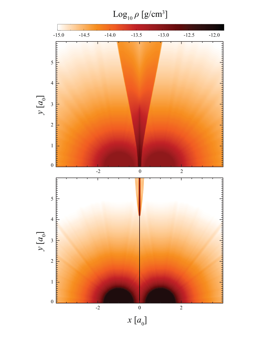
Figure 1.— Density structures resulting from the instantaneous acceleration model (top), and from the accelerating wind model (bottom) with a $\beta$-law profile ($\beta=1$). $x$-$y$ axis are in units of $a_{0}=a/2$, which is the distance from one star to the contact discontinuity along the orbital plane. Following Stevens et al. (1992) we calculate the cooling parameter $\chi=t_{\rm cool}/t_{\rm dyn}$ as function of $y$, with $t_{\rm cool}=kT_{s}/4n_{w}\Lambda(T_{s})$, where $n_{w}$ and $T_{s}$ are the pre-shock density and shock temperature respectively (both functions of $r$), and $t_{\rm dyn}=x_{0}/c_{s}$, with $x_{0}=a/2$ being the distance from one star to the contact discontinuity and $c_{s}$ the sound speed. The cooling appears to be efficient ($\chi<1$) up to $y/x_{0}\approx 4$, which is reflected in the structure of the wind-wind interaction region shown in the bottom panel

.

2.2. X-ray Lightcurves

The results from the hydrodynamic simulations are used to construct both density and temperature profiles for the X-ray emitting material along the $y$-axis by averaging over the width of the shocked region ($x$-axis). The thermodynamical profiles are then used as initial conditions for the radiative transfer code Cloudy 13.00 (Ferland et al., 2013) to determine emissivity and opacity profiles for the shocked wind gas in the 0.1 - 10 keV energy range with 240 logarithmically spaced energy bins. Assuming cylindrical symmetry we are able to construct three-dimensional maps of the shocked and unshocked gas.

The opacity for the unshocked material is calculated using Cloudy under the assumption that the outflowing wind from each star is irradiated by a stellar blackbody chosen to match the observed properties of the binary (Table1). In addition to the stellar radiation field, a central X-ray source characterized by a thermal bremsstrahlung spectrum with $T_{\rm ff}$ and $L_{\rm ff}$ was also included. The values of $T_{\rm ff}$ and $L_{\rm ff}$ are chosen to closely match the total unabsorbed radiation emitted by the shocked region, although as shown by Antokhin et al. (2004), the opacity of the cold wind material at the energy ranges where the X-ray lightcurves are constructed is not sensitive to the properties of the X-ray emission. Finally, X-ray lightcurves for the entire orbit are constructed by ray-tracing the emitted radiation from the shocked region over the three-dimensional wind gas maps, which are assumed to be inclined with respect to the observer at an angle $i$ (see Table 1).

3. The Gas and X-ray Emission Properties

3.1. The Wind-Wind Interaction Region

The results of our simulations are shown in Figure 1 for the two different models. In the velocity profile model, the lower pre-shock velocities and the corresponding larger pre-shock densities result in a sizable increase in the post-shock densities (with respect to the instant acceleration model) which, together with the accompanying lower post-shock temperatures lead to efficient radiative cooling in the inner regions. As shown in Figure 1, this sizable increase in energy loss causes the shocked wind material to compress into a thin layer up to a height of about $y/x_{0}\approx 4$ where cooling becomes less efficient.

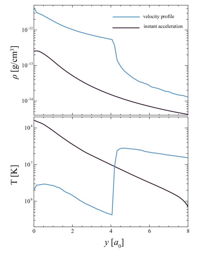
Figure 2.— Density and temperature profiles within the shocked material, obtained by averaging over the width of the shocked region ($x$-axis), for the instant acceleration (black line) and velocity profile (blue line) models, respectively. At $y/x_{0}<4$, a clear temperature inversion layer is produced in the velocity profile model as a result of the corresponding larger post-shock densities and lower post-shock temperatures, which lead to more efficient radiative cooling with respect to the instant acceleration model.

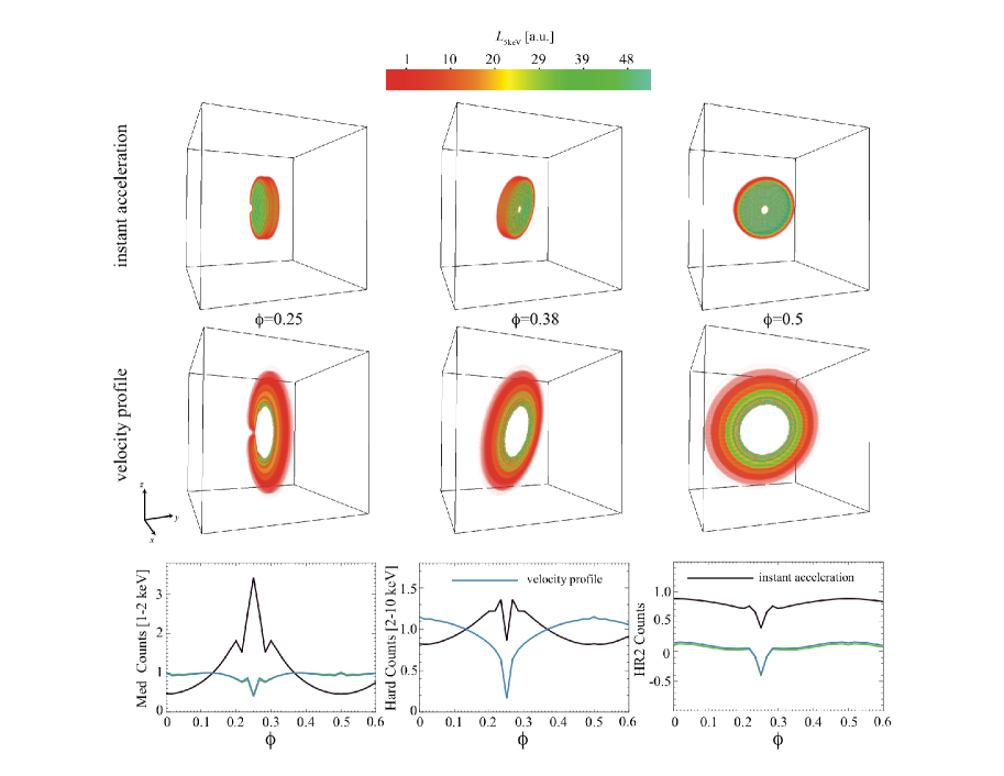
Figure 3.— Intensity maps (in arbitrary units) at 5 keV for model the instant acceleration and velocity profile models at orbital phases $\phi=$ 0.25, 0.38, and 0.5 (from left to right). Bottom Panels: Lightcurves at medium (left) and hard (middle) bands, and for the hardness ratio (right) as predicted from the instant acceleration and velocity profile models. Counts are 5 ks bins. Lightcurves are normalized to $\phi=0.37$, between eclipsing and conjunction phases. The green lines shows the lightcurves for the case in which the opacity of the unshocked wind material was calculated using the stellar blackbodies as illuminating sources. To examine how X-ray radiation affects the absorption cross section, the bottom panels also includes a model (blue lines) with an added bremsstrahlung component ($T_{\rm ff}=3\times 10^{7}$ K and $L_{\rm ff}=10^{34}$ erg s^-1). Here $T_{\rm ff}$ and $L_{\rm ff}$ were chosen to closely match the total unabsorbed X-ray radiation, although we found that the opacity of the wind at the energy ranges where the lightcurves are constructed is not appreciably altered by the specific spectrum and intensity of the illuminating X-ray source. As can be clearly seen, there is no discernible differences between the green and blue lines in the hard band and only minute differences in the medium band.

In this way, in the central regions of the shocked wind ($y/x_{0}<4$), the temperature in the velocity profile model remains below $\sim 10^{6}$ K (Figure 2), such that this material does not contribute to the X-ray emission at energies above 0.1 keV. The main contribution to the X-ray luminosity in the velocity profile model thus arises from layers within the shocked wind region located at distances that are significantly larger than the binary separation and, as a result, are not eclipsed by the stars. What is more, due to the clear temperature inversion in the velocity profile model, emission at softer X-ray energies (which is more readily absorbed by the stellar wind gas) is produced in layers that are located deeper within the shocked wind region that those emitting higher energy X-rays. As we will discuss in Section 3.2, both of these effects have important consequences on the resulting X-ray lightcurves.

3.2. X-ray Lightcurves

The behavior of the lightcurves depends on the thermodynamical structure of the shocked region and the opacity of the unshocked wind material. The lightcurves for the medium ($M$: 1-2 keV) and hard ($H$: 2-10 keV) bands, and for the hardness ratio $HR_{2}=(H-M)/(H+M)$ are calculated by ray-tracing the emission from the shocked wind region over the three-dimensional gas maps. In Figure 3 we compare the intensity of the emitting regions contributing to the observed luminosity at 5 keV for the two different wind initiation models. In the case of the velocity profile model, the hot gas contributing with the bulk of the X-ray luminosity is no longer confined midway between the stars (top row) but it is located in an extended, ring-like structure (middle row) and, as a result, the emission is not drastically absorbed by the stars and their close-by winds. In the instant acceleration model, on the other hand, the confinement of the emitting region midway between the stars causes the X-ray lightcurve to show prominent eclipses ($\phi=0,0.5$).

In the velocity profile model, the majority of the soft X-ray emission arises in layers that are deeper within the shocked region than in the instant acceleration model (Figure 2). This causes more efficiently absorption at all orbital phases, which is reflected in the shape of the resulting lightcurve, which in the medium X-ray band, becomes much flatter than in the instant acceleration model (Figure 3). In addition, the density in the shocked region is significantly increased in the velocity profile model, causing a sizable increase in the total column density along the contact discontinuity. This increase in optical depth causes a sharp decrease in the X-ray luminosity when $\phi=0.25$ at both hard and medium energies. This decrement is then followed by a steady increase in X-ray luminosity as the optical eclipses are taken place ($\phi=0,0.5$) and is more pronounced at medium X-ray energies (Figure 3).

It is important to note that in the instant acceleration model, because the softer X-ray emission arises from more distant (and less opaque) layers within the shocked region (Figure 2), the medium X-ray band light curve shows a sizable increase in luminosity at $\phi=0.25$ when softer photons emitted from the shocked wind region can reach the observer without transversing the cold, more opaque wind. As a consequence of both the decrease in temperature and increase in absorption within the shock wind region, the global emission becomes softer in the velocity profile model as can be seen in the comparison of the hardness ratio depicted in Figure 3. The total observed luminosities in the 1-10 keV energy range for the instant acceleration and velocity profile models are $L_{X}=1.13\times 10^{35}(d/8~{}{\rm kpc})^{2}\;$erg s^-1 and $L_{X}=1.86\times 10^{34}(d/8~{}{\rm kpc})^{2}\;$erg s^-1, respectively. Having laid the foundation for how the size and structure of the shocked and unshocked regions are shaped by the wind initiation properties, we now turn our attention to whether the simulated flow properties can robustly explain salient X-ray observational features of WR 20a.

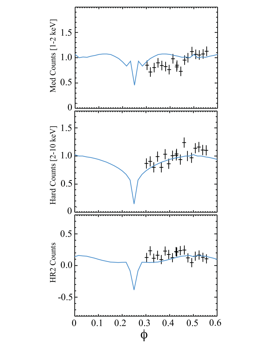
Figure 4.— Comparison between lightcurve predicted by the velocity profile model (black line) and the observed X-ray lightcurve reported by Nazé et al. (2008). Medium, hard and hardness ratio (from top to bottom) are displayed. Counts are 5 ks bins. Lightcurves are normalized to the $\phi=0.47$, the intermediate phase at which observations were taken. The total observed luminosity in the 1-10 keV energy range predicted for this model is $L_{X}=1.8\times 10^{34}(d/8~{}{\rm kpc})^{2}\;$erg s^-1. This should be compared to $L_{X}=5.17=\times 10^{33}(d/8~{}{\rm kpc})^{2}$ erg s^-1, the unabsorbed luminosity derived by Nazé et al. (2008), although caution must be taken as this estimate was derived assuming only Galactic absorption.

4. Discussion

In this work, we have presented a simplified formalism for modeling the relative complexity of the stellar wind initiation and interaction in the massive, close binary WR 20a. Despite its simplicity, this model can successfully reproduce the observations. In Figure 4, we compare our velocity profile model predictions to the Chandra lightcurves of WR 20a obtained by Nazé et al. (2008). Overall, the predicted X-ray lightcurves show no significant flux decrement during secondary optical eclipse but instead appear more luminous and softer as the shock-wind region is observed face on. Notably, such features are only present in models when the emanating wind is assumed to be accelerated (Figure 3). This system provides a direct diagnostic of the stellar wind initiation and suggests that more detailed observations of WR 20a could help to constrain answers related to the currently unsolved problem of how WR stars can drive such strong winds (Owocki, 2011).

As observed in Figure 4, our models not only explain current Chandra observations but provide detailed predictions over the entire orbital phase. With a more precise estimate of $d$ (the distance to the source) and a better orbital phase monitoring characterization, the approach presented here may be extended to explore several interesting questions. In particular, we have considered the idealized case in which the structure of the shocked wind region is not affected by the orbital motion, we have assumed that the wind profile is characterized by $\beta=1$ (Rauw et al., 2005) and have neglected the additional pressure provided by the WR-star light, which is expected to lead to a radiative braking of the impacting WR wind. As observations improve, three-dimensional simulations of WR 20a with different velocity profiles will be needed to test two-dimensional results and analyze how projection effects can alter our interpretation of both structures and lightcurves.

While it is important to investigate the behavior of individual objects, we should not lose sight of the common physical processes involved. There has been detailed hydrodynamical models aimed at understanding the X-ray lightcurves of WR+O stars: $\eta$ Carinae (Parkin et al., 2009; Okazaki et al., 2008; Corcoran et al., 2010), WR 140 (Corcoran et al., 2011) and WR 22 (Parkin & Gosset, 2011), which in some case have separations of only a few O-star radii. Generally the WR wind in these systems is so much stronger that it is expected to overwhelm its companion’s outflow. Orbital phase monitoring of such systems suggests that contrary to what a simple hydrodynamic ram balance between the two stars might suggest the wind-wind interface is generally kept away from the O-star surface, possibly due to the additional pressure provided by the O-star light impacting the WR wind (Gayley et al., 1997; Parkin et al., 2009). It is of course interesting to study these systems as they appear to be rather common, but it would be better to use simpler systems like WR 20a as proving grounds of the relative complexity of WR wind initiation.

References

- Abbott et al. (1986) Abbott, D. C., Beiging, J. H., Churchwell, E., & Torres, A. V. 1986, ApJ, 303, 239
- Antokhin et al. (2004) Antokhin, I. I., Owocki, S. P., & Brown, J. C. 2004, ApJ, 611, 434
- Bonanos et al. (2004) Bonanos, A. Z., Stanek, K. Z., Udalski, A., et al. 2004, ApJ, 611, L33
- Cappa et al. (2004) Cappa, C., Goss, W. M., & van der Hucht, K. A. 2004, AJ, 127, 2885
- Castor et al. (1975) Castor, J. I., Abbott, D. C., & Klein, R. I. 1975, ApJ, 195, 157
- Chlebowski et al. (1989) Chlebowski, T., Harnden, F. R., Jr., & Sciortino, S. 1989, ApJ, 341, 427
- Corcoran et al. (2010) Corcoran, M. F., Hamaguchi, K., Pittard, J. M., et al. 2010, ApJ, 725, 1528
- Corcoran et al. (2011) Corcoran, M. F., Pollock, A. M. T., Hamaguchi, K., & Russell, C. 2011, arXiv:1101.1422
- De Colle & Raga (2006) De Colle, F., & Raga, A. C. 2006, A&A, 449, 1061
- De Colle et al. (2008) De Colle, F., Raga, A. C., & Esquivel, A. 2008, ApJ, 689, 302
- De Colle et al. (2012) De Colle, F., Granot, J., López-Cámara, D., & Ramirez-Ruiz, E. 2012, ApJ, 746, 122
- Dalgarno & McCray (1972) Dalgarno, A., & McCray, R. A. 1972, ARA&A, 10, 375
- Ferland et al. (2013) Ferland, G. J., Porter, R. L., van Hoof, P. A. M., et al. 2013, RMxAA, 49, 137
- Gräfener & Hamann (2005) Gräfener, G., & Hamann, W.-R. 2005, A&A, 432, 633
- Gayley et al. (1997) Gayley, K. G., Owocki, S. P., & Cranmer, S. R. 1997, ApJ, 475, 786
- Lucy & White (1980) Lucy, L. B., & White, R. L. 1980, ApJ, 241, 300
- Montes et al. (2009) Montes, G., Pérez-Torres, M. A., Alberdi, A., & González, R. F. 2009, ApJ, 705, 899
- Nazé et al. (2008) Nazé, Y., Rauw, G., & Manfroid, J. 2008, A&A, 483, 171
- Nazé (2009) Nazé, Y. 2009, A&A, 506, 1055
- Okazaki et al. (2008) Okazaki, A. T., Owocki, S. P., Russell, C. M. P., & Corcoran, M. F. 2008, MNRAS, 388, L39
- Owocki (2011) Owocki, S. 2011, Bulletin de la Societe Royale des Sciences de Liege, 80, 16
- Pittard & Corcoran (2002) Pittard, J. M., & Corcoran, M. F. 2002, A&A, 383, 636
- Pittard & Parkin (2010) Pittard, J. M., & Parkin, E. R. 2010, MNRAS, 403, 1657
- Parkin et al. (2009) Parkin, E. R., Pittard, J. M., Hoare, M. G., Wright, N. J., & Drake, J. J. 2009, MNRAS, 400, 629
- Parkin & Gosset (2011) Parkin, E. R., & Gosset, E. 2011, A&A, 530, A119
- Pittard (2009) Pittard, J. M. 2009, MNRAS, 396, 1743
- Pollock et al. (2005) Pollock, A. M. T., Corcoran, M. F., Stevens, I. R., & Williams, P. M. 2005, ApJ, 629, 482
- Rauw et al. (2005) Rauw, G., Crowther, P. A., De Becker, M., et al. 2005, A&A, 432, 985
- Sana et al. (2006) Sana, H., Gosset, E., & Rauw, G. 2006, MNRAS, 371, 67
- Skinner et al. (2012) Skinner, S. L., Zhekov, S. A., Güdel, M., Schmutz, W., & Sokal, K. R. 2012, AJ, 143, 116
- Stevens et al. (1992) Stevens, I. R., Blondin, J. M., & Pollock, A. M. T. 1992, ApJ, 386, 265
- Usov (1992) Usov, V. V. 1992, ApJ, 389, 635