Exploring the Milky Way stellar disk

Abstract

Aims. The aim of this paper is to explore and map the age and abundance structure of the stars in the nearby Galactic disk.

Methods. We have conducted a high-resolution spectroscopic study of 714 F and G dwarf and subgiant stars in the Solar neighbourhood. The star sample has been kinematically selected to trace the Galactic thin and thick disks to their extremes, the metal-rich stellar halo, sub-structures in velocity space such as the Hercules stream and the Arcturus moving group, as well as stars that cannot (kinematically) be associated with either the thin disk or the thick disk. The determination of stellar parameters and elemental abundances is based on a standard 1-D LTE analysis using equivalent width measurements in high-resolution ($R=40\,000-110\,000$) and high signal-to-noise ($S/N=150-300$) spectra obtained with FEROS on the ESO 1.5-m and 2.2-m telescopes, SOFIN and FIES on the Nordic Optical Telescope, UVES on the ESO Very Large Telescope, HARPS on the ESO 3.6-m telescope, and MIKE on the Magellan Clay telescope. NLTE corrections for individual Fe i lines were employed in every step of the analysis.

Results. We present stellar parameters, stellar ages, kinematical parameters, orbital parameters, and detailed elemental abundances for O, Na, Mg, Al, Si, Ca, Ti, Cr, Fe, Ni, Zn, Y, and Ba for 714 nearby F and G dwarf stars. Our data show that there is an old and $\alpha$-enhanced disk population, and a younger and less $\alpha$-enhanced disk population. While they overlap greatly in metallicity between $\rm-0.7<[Fe/H]\lesssim+0.1$, they show a bimodal distribution in $\rm[\alpha/Fe]$. This bimodality becomes even clearer if stars where stellar parameters and abundances show larger uncertainties ($T_{\rm eff}\lesssim 5400$ K) are discarded, showing that it is important to constrain the data set to a narrow range in the stellar parameters if small differences between stellar populations are to be revealed. We furthermore find that the $\alpha$-enhanced population has orbital parameters placing the stellar birthplaces in the inner Galactic disk while the low-$\alpha$ stars mainly come from the outer Galactic disk, fully consistent with the recent claims of a short scale-length for the $\alpha$-enhanced Galactic thick disk. We have also investigated the properties of the Hercules stream and the Arcturus moving group and find that neither of them present chemical or age signatures that could point to that they are disrupted clusters or extragalactic accretion remnants from ancient merger events. Instead, they are most likely dynamical features originating within the Galaxy. We furthermore have discovered that a standard 1-D, LTE analysis, utilising ionisation and excitation balance of Fe i and Fe ii lines produces a flat lower main sequence. As the exact cause for this effect is unclear we chose to apply an empirical correction. Turn-off, and more evolved, stars, appears to be un-affected.

1 Introduction

How galaxies form and evolve is a vast subject that has in the last decades rapidly developed into one of the most exciting areas in contemporary astrophysics. The goal has been to unveil the mysteries of the formation, assembly and chemical history of galaxies, and our own galaxy, the Milky Way, in particular. As the Milky Way currently is the only galaxy whose stellar populations can be studied in great detail with high-resolution spectrographs, and may serve as a “benchmark galaxy” for extra-galactic studies, it is essential to establish the properties of the different Milky Way stellar populations.

Major pieces to the puzzle of galaxy formation are held by the atmospheres of stars which may remain intact over time and act as time capsules showing the mixture of chemical elements that were present in the gas cloud out of which the stars formed billions of years ago (e.g., Lambert 1989; Freeman & Bland-Hawthorn 2002). F and G dwarf stars are especially reliable tracers as their expected lifetimes on the main sequence, burning hydrogen to helium in their centres, are similar to, or possibly even longer than, the current age of the Galaxy. For instance, a solar-type star will spend around 10 Gyr on the main sequence (e.g., Sackmann et al. 1993). During this time its atmosphere is untouched by internal nuclear processes. By obtaining high-resolution spectra of such stars it is possible to determine their detailed chemical compositions and ages, which allow us to trace the histories of different stellar populations. In the last 20 years, several studies have aimed at characterising the Galactic stellar disk using nearby F and G dwarf stars (e.g., Edvardsson et al. 1993; Feltzing & Gustafsson 1998; Fuhrmann 1998, 2000, 2004, 2008, 2011; Prochaska et al. 2000; Gratton et al. 2000; Chen et al. 2000; Mashonkina & Gehren 2001; Tautvaišienė et al. 2001; Trevisan et al. 2011; Bensby et al. 2003, 2004b, 2005, 2007b; Bensby & Feltzing 2006; Feltzing et al. 2007; Soubiran et al. 2003; Reddy et al. 2003, 2006). The evidence from these high-resolution spectroscopic studies have so far shown that the Milky Way appears to contain two disk populations, with different chemical and age properties, indicating different origins and different chemical histories.

However, after more than two decades of observational efforts, we are still lacking much information about the complex abundance structure of the Galactic stellar disk. For instance, the Geneva-Copenhagen Survey (hereafter GCS) by Nordström et al. (2004) contains approximately 14 000 dwarf stars in the Solar neighbourhood, all of which have full three-dimensional kinematic information available, as well as ages and metallicities estimated from Strömgren photometry. It is evident from the GCS data that there are substantial kinematical sub-structures present in the Solar neighbourhood that can be associated with various stellar streams and moving groups (e.g., Nordström et al. 2004; Navarro et al. 2004; Famaey et al. 2005; Soubiran & Girard 2005; Arifyanto & Fuchs 2006; Helmi et al. 2006). These kinematical substructures, seen in the immediate Solar neighbourhood, have recently been confirmed to persist to distances of at least 1 kpc from the Sun, although with slightly shifted velocity components (Antoja et al. 2012). It is unclear whether such structures are of Galactic or extragalactic origin. The GCS also contains many stars with typical thick-disk kinematics, and with very high metallicities, well above solar (cf. Figs. 1 and 3). The question is whether these stars are true thick disk stars. It is also unclear what the lowest metallicities are in the thin disk, and whether the thin and thick disks show distinct abundance trends.

In addition, recent studies of the SDSS Segue G and K dwarf stellar sample by Abazajian et al. (2009); Yanny et al. (2009) of more than 5000 stars at larger distances add a new dimension to this discussion. From this data (but treated in different ways) Bovy et al. (2012) finds that there is no distinct thick disk, whilst Lee et al. (2011) and Liu & van de Ven (2012) find two or perhaps even three components in the stellar disk. Furthermore, other recent studies actually show that many, if not all, edge-on spiral galaxies appear to host dual disk systems (e.g., Yoachim & Dalcanton 2006; Comerón et al. 2011).

Distinct and different multiple stellar disks are an important component in galaxy formation models, and the signature of a unique thick disk in such models depends on the formation scenario. For example, if radial migration is the responsible mechanism, then it is a continuous process and the result could very well be that the thick and thin disks form a smooth transition. On the other hand, if the formation of the thick disk is fast, e.g., through kinematical heating of an old disk due to an ancient merger event, it is more likely that the two disks are distinct components in chemistry and phase-space (Minchev et al. 2012). It is therefore extra important that the dichotomy of the Milky Way stellar disk is well-understood, helping us to better understand galaxy formation in general.

On larger scales, there are several ongoing and upcoming large spectroscopic surveys that will probe the abundance structure of the Milky Way and its stellar populations on much larger scales. Examples are the SDSS Segue (Yanny et al. 2009), APOGEE (Allende Prieto et al. 2008), the Gaia-ESO Survey (Gilmore et al. 2012), the GALAH survey (e.g., Zucker et al. 2012) which together will gather spectra and determine stellar parameters and chemical abundances for several hundreds of thousands of dwarf and red giant stars in the Galactic thin disk, thick disk, stellar halo, and bulge. However, these surveys are based on low- or medium-resolution spectra that often have very limited wavelength coverages and sometimes lower signal-to-noise ratios. Hence, they will need to anchor their results to studies that present detailed elemental abundances that have been homogeneously determined from high-resolution and high signal-to-noise spectra.

Figure 1: The kinematical thick disk-to-thin disk probability ratio ($TD/D$) versus metallicity for the $\sim 14000$ stars in the GCS. Stars with $TD/D>2$ are, to a first approximation, classified as potential thick disk stars, and stars with $TD/D<0.5$ are, to a first approximation, classified as potential thin disk stars. Stars with probability ratios between these two limits are here classified as “in-between stars”. Note that all metallicities, [M/H], are from the Strömgren calibration by Casagrande et al. (2011).

The stellar sample presented in this study aims at mapping and exploring the age and abundance structure of the Milky Way stellar disk in a consistent and homogeneous way based on high-resolution and high signal-to-noise spectra of nearby F and G dwarf stars. In this paper we describe the star sample and the elemental abundance analysis, as well as presenting the observed properties of the Galactic disk. In particular, the extent and variation of elemental abundances and stellar ages with galactocentric radius is explored.

First results based on the current sample have been published in Bensby et al. (2007a, b); Feltzing & Bensby (2008); Bensby & Feltzing (2010), and the sample has also been part of the recalibration of the Geneva-Copenhagen Survey (Casagrande et al. 2010), characterisation of planet signatures in solar-type stars (Ramírez et al. 2010), and most recently in the chemical tagging experiment by Mitschang et al. (2013). Further investigations into the dichotomy of the Galactic stellar disk are conducted in a parallel paper (Feltzing et al. 2013, in preparation), while work on odd iron peak elements will be presented in Battastini & Bensby (in preparation), and results for a larger range of $r-$ and $s-$process elements in Battistini et al., (in preparation).

2 Sample selection

Figure 2: (a) The $TD/D$ distribution of our sample of 714 stars. The solid vertical lines mark the $TD/D=0.5$ and $TD/D=2$ ratios. Panels (b)–(d) show the metallicity distributions of 239 potential thick disk stars with $TD/D>2$, out of which 36 stars have $TD/H<1$, i.e. most likely halo stars; 88 stars with kinematics “in between”; and the 387 potential thin disk stars with $TD/D<0.5$. In (a) and (b) the likely halo stars ($TD/H<1$) are marked by solid black histograms. The metallicities are from our spectroscopic analysis.

Figure 3: 690 out of 714 stars in our sample are also present in the GCS. The figure shows $U_{\rm LSR},\,V_{\rm LSR},\,W_{\rm LSR}$ velocities versus [M/H] for the $\sim 14000$ stars in the GCS (grey dots), and open circles show our stars (those with $\rm[M/H]>-2$). Note that all metallicities, [M/H], are from the Strömgren calibration by Casagrande et al. (2011).

The star sample presented here results from the joint effort of several observing campaigns with different aims. In particular, we wanted to trace the metal-poor limit of the thin disk, the metal-rich limit of the thick disk, the metal-poor limit of the thick disk, the metal-rich limit of the stellar halo, structures in velocity space such as the Hercules stream and the Arcturus moving group, and stars that have kinematical properties placing them in between those of the thin and thick disks. Hence, our selection function is very complex and the sample should not be used to determine the distributions of their properties such as velocity, age, and metallicity.

For the selections of candidate members of the different stellar populations, we used the kinematical criteria defined in Bensby et al. (2003), i.e. assuming that they have Gaussian velocity distributions, different rotation velocities around the Galactic centre, and occupy certain fractions of the stellar content of the Solar neighbourhood. A shortcoming of this kinematical approach is the assumption that the distributions follow normal distributions. As noted in Ruchti et al. (2010) these are first order approximations and the real functions may be more complex, which can also be seen in the GCS (Nordström et al. 2004), where the velocity distributions are clearly not Gaussian. A better understanding of the distribution functions may lead to a better decomposition of the stellar disk into sub-components (Binney 2010). However, for our purposes, these kinematical criteria are, together with the metallicities [M/H] from the GCS, a sufficient starting point to probe the thin and thick disks to their extremes.

Figure 4: Toomre diagram of our program stars. (a) shows the full range of velocities while (b) zooms in on the region where a majority of the sample is located. Dotted lines show constant values of the total space velocity, $v_{tot}=(U_{\rm LSR}^{2}+V_{\rm LSR}^{2}+W_{\rm LSR}^{2})^{1/2}$, in steps of 100 ${\rm\,km\,s^{-1}}$ and $50\,{\rm\,km\,s^{-1}}$, respectively, in the two plots.

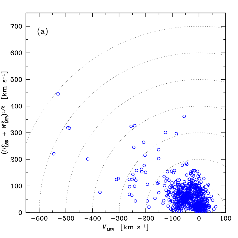
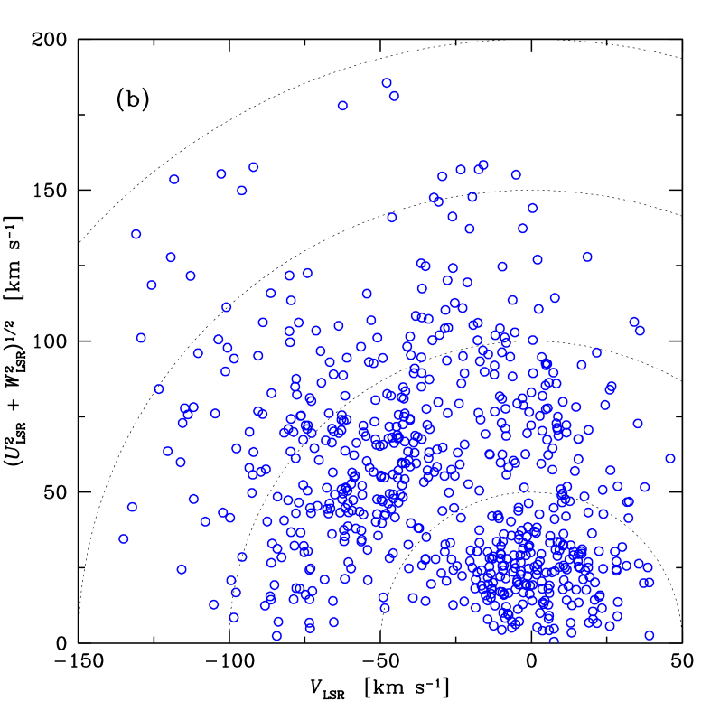
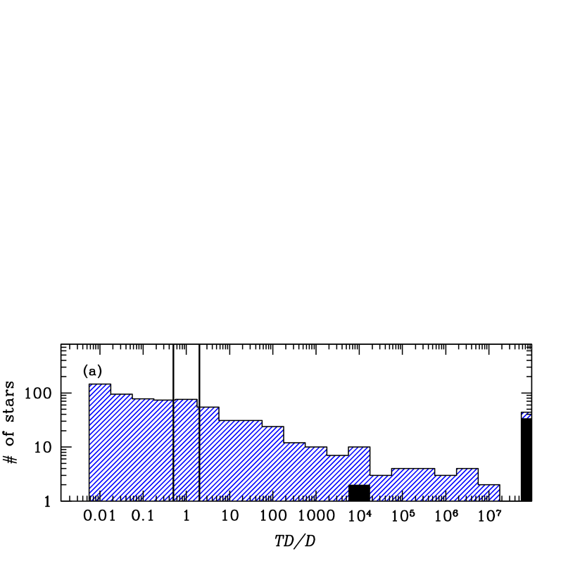
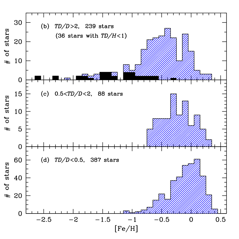
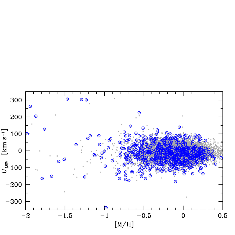
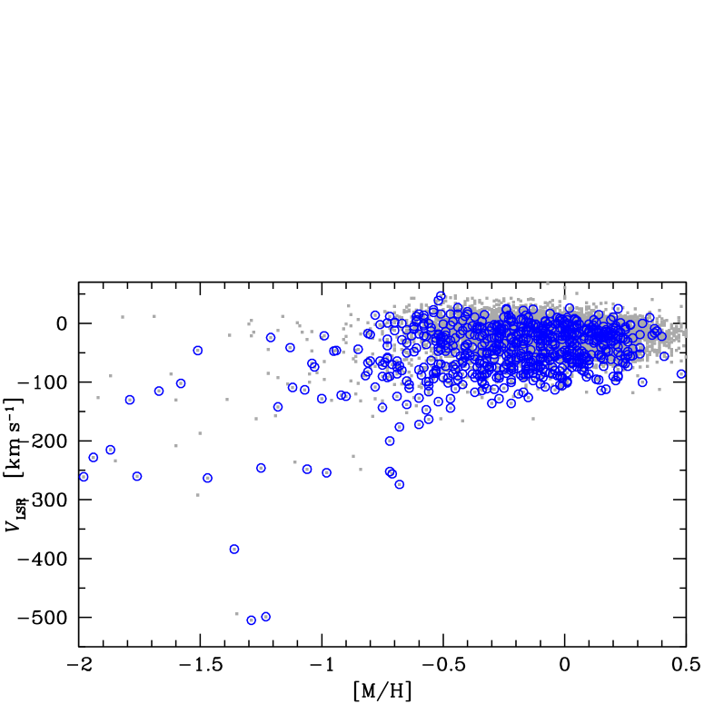
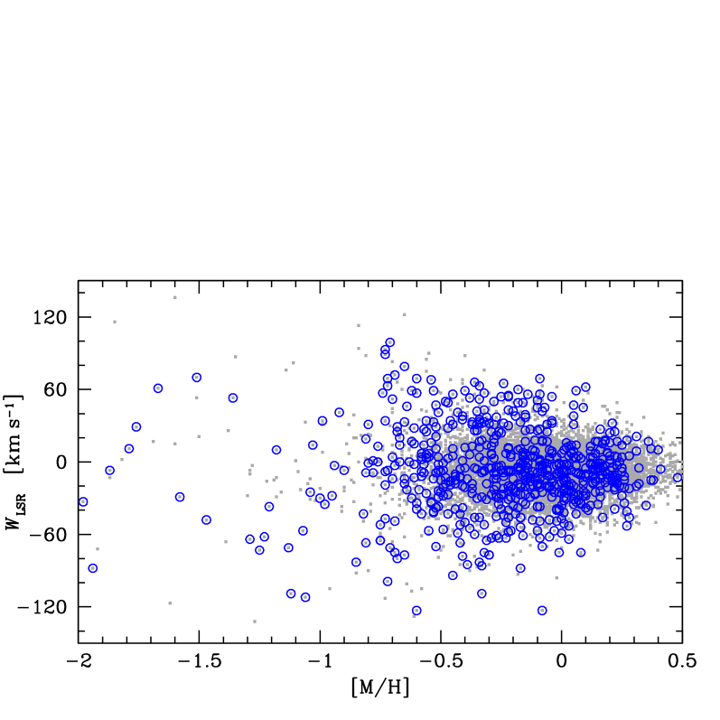
Figure 1 shows the thick-to-thin disk probability ratios ($TD/D$) versus the photometric metallicity, [M/H], from Casagrande et al. (2011) for the $\sim$14 000 stars in the GCS. For a star to be a candidate thick disk star, we require it to have a probability at least two times that of being a thin disk star ($TD/D>2$), and vice versa for a candidate thin disk star $TD/D<0.5$. These probability ratios are marked by the two horizontal lines in Fig. 1. This plot is typical for how the candidate thin and thick disk stellar samples were selected. The $TD/D$ distribution of our sample of 714 stars is shown in Fig. 2a, and according to these kinematical criteria we have 387 stars with thin disk kinematics ($TD/D<0.5$), 203 stars with thick disk kinematics ($TD/D>2$), 36 stars with halo kinematics ($TD/H<1$), and 89 stars with kinematics in between those of the two disks. Note that the probability ratios presented here are based on the thin and thick disk normalisations and velocity dispersions given in Table 4. As these numbers change, the $TD/D$ probability ratios will also change. For instance, the recent models by Binney (2012) show that the thick disk might be kinematically hotter vertically than radially, which is opposite to expectation from the numbers given in Table 4. The numbers given here merely reflect the way our sample was selected. The metallicity distributions of the three $TD/D$ samples are shown in Fig. 2b–d. There is a large overlap in metallicity between them. The full sample of 714 stars is further shown in Fig. 3 where the $U_{\rm LSR}$, $V_{\rm LSR}$, and $W_{\rm LSR}$ velocities are plotted versus metallicity, with all the GCS stars as grey dots in the background. From these plots it is evident that our sample probes the whole GCS, and that we sample the extreme kinematics/metallicities; the sample contains many stars with hot kinematics at high metallicities and many stars with cold kinematics at low metallicities. Please note that the very highest metallicities in the plots in Fig. 3 in fact may not correspond to high iron abundance but may result from a limitation of photometric metallicity calibrations.

Another way of displaying the sample is by a Toomre diagram, which is a representation of the combined vertical and radial kinetic energies versus the rotational energy. This is shown for the 714 stars in Fig. 4. Low-velocity stars, within a total velocity $v_{\rm tot}\equiv(U_{\rm LSR}^{2}+V_{\rm LSR}^{2}+W_{\rm LSR}^{2})^{1/2}$ of $50\,{\rm\,km\,s^{-1}}$ are, to a first approximation, mainly thin disk stars, and stars with $70\lesssim v_{\rm tot}\lesssim 180\,{\rm\,km\,s^{-1}}$ are likely to be thick disk stars (e.g., Nissen 2004). Stars with $v_{\rm tot}>200\,{\rm\,km\,s^{-1}}$ are likely halo stars. The slight excess of stars in Fig. 4 with $V_{\rm LSR}\approx-50\,{\rm\,km\,s^{-1}}$ and $(U^{2}+W^{2})^{1/2}\approx 50-70\,{\rm\,km\,s^{-1}}$ is present because we have deliberately targeted stars that can be associated with the Hercules stream (e.g., Famaey et al. 2005; Bensby et al. 2007a)

Please note that first results based on the current sample of 714 stars were published in Bensby et al. (2007a) about the Hercules stream (60 stars) and in Bensby et al. (2007b) about the metal-rich limit of the thick disk (169 stars). The 102 stars from Bensby et al. (2003, 2005) are also present in the current sample. No tables or results for individual stars have been published in the two letters in 2007, that only referred to the upcoming full publication (which is this paper). Hence we consider the data for all stars (except the 102 stars from Bensby et al. 2003, 2005, but those have been re-analysed here) as new.

3 Space velocities and galactic orbits

Space velocities, $U_{\rm LSR}$, $V_{\rm LSR}$, and $W_{\rm LSR}$, were calculated using positions from the Hipparcos catalogue (ESA 1997), parallaxes from the new reduction of the Hipparcos data by van Leeuwen (2007), proper motions from the Tycho-2 catalogue (Høg et al. 2000), and radial velocities from Nordström et al. (2004) and, if not available in the GCS, from Barbier-Brossat et al. (1994) or Barbier-Brossat & Figon (2000). To relate the space velocities to the Local Standard of Rest (LSR), the Sun’s velocity components relative to the LSR $(U_{\sun},\,V_{\sun},\,W_{\sun})=(11.10,\,12.24,\,7.25)\,{\rm\,km\,s^{-1}}$ from Schönrich et al. (2010) were added.

Galactic orbits were then calculated with the grinton integrator (Carraro et al. 2002; Bedin et al. 2006) which uses the Milky Way potential model by Allen & Santillan (1991). The model is time-independent, axisymmetric, fully analytic, and consists of a spherical central bulge, a disk, a massive spherical halo, and has a total mass of $9\times 10^{11}$ solar masses. When calculating $X,\,Y,\,{\rm and}\,Z$ for the stars, 8.5 kpc was adopted as the Sun’s distance to the Galactic centre, and 20 pc for the Sun’s distance above the Galactic plane (Humphreys & Larsen 1995; Joshi 2007). Output parameters from grinton are: the minimum and maximum distances from the Galactic centre $R_{\rm min}$ and $R_{\rm max}$ (i.e., the peri- and apocentric values); the maximum distance from the Galactic plane $Z_{\rm max}$; the eccentricity, $e=(R_{\rm max}-R_{\rm min})/(R_{\rm max}+R_{\rm min})$; the total energy $E_{\rm tot}$; and the angular momentum $L_{z}$. Figure 5 shows the total energy - angular momentum plot (also commonly referred to as a Lindblad plot) for the sample. As the value of $E_{\rm tot}$ is dependent on how the Galactic potential is normalised, and may be difficult to compare between studies, we chose to normalise $E_{\rm tot}$ to the LSR, giving $E/E_{\rm LSR}$. The parameters are listed for all stars in Table 7 in the Appendix.

Figure 5: Energy versus angular momentum $L_{Z}$. The energy has been normalised to the local standard of rest (LSR), which is marked by the white circle and the dotted lines.

Table 1: Observing runs.^†

Telescope	Instrument	$R$	Obs. mode	Date	# of stars	Sun
ESO 1.5-m	FEROS	48 000	visitor	2000 Sep	3100	-
”	”	48 000	visitor	2001 Aug.	3100	Sky
ESO 2.2-m	FEROS	48 000	service	2005/2006	2900	-
ESO 3.6-m	HARPS	120 000	visitor	2009 March	500
VLT	UVES	110 000	visitor	2002 Jul	400	-
”	”	110 000	service	2003/2004	2300	-
”	”	80 000	archive	UVES POP	3100	Sky‡
NOT	SOFIN	80 000	visitor	2002 Aug	1100	-
”	”	80 000	visitor	2002 Nov.	1600	Moon
”	”	80 000	service	2003 June	900	-
”	”	80 000	service	2004 Feb.	500	-
”	”	80 000	service	2006 March	1100	-
NOT	FIES	67 000	visitor	2008 July, Nov.	600
Magellan	MIKE	65 000	visitor	2005 Aug.	6100	-
”	”	65 000	visitor	2006 Jan.	7400	Vesta
”	”	65 000	visitor	2006 April	8100	Ganymede
”	”	65 000	visitor	2006 Aug.	15800	Ceres
”	”	42 000	visitor	2007 April	4900	Ganymede
”	”	55 000	visitor	2007 May	600	-
”	”	55 000	visitor	2007 July	1300	-
”	”	55 000	visitor	2007 Nov.	6000	-

4 Observations

High-resolution and high signal-to-noise spectra of 848 nearby F and G dwarf and subgiant stars in the Solar neighbourhood were obtained during several observing runs between 2000 and 2009. Another 48 spectra were gathered from the ESO UVES POP database, giving a sample of, in total, 885 stars. A significant number (198) of the stars turned out to be spectroscopic binaries and/or had too wide spectral lines due to too high projected rotational velocities ($v\sin i$), making them unsuitable for detailed elemental abundance analysis based on equivalent width measurements. The final stellar sample we analyse, and for which stellar parameters, elemental abundances and stellar ages were determined, consists of 714 F and G dwarf stars. Table 5 in the Appendix lists the rejected stars and the reasons for which they were rejected.

For the first observing runs, between 2000 and 2002 with FEROS and SOFIN, the stars were selected from the catalogue by Feltzing et al. (2001). Those 102 stars were published in Bensby et al. (2003, 2005). The stars from observing runs in 2003 and onwards were selected from the GCS. Except for 16 stars (from the first FEROS and SOFIN runs), all stars in the current sample of 714 stars are present in the GCS.

Table 1 lists the different observing runs and additional details regarding the spectrographs and data reductions are given below:

FEROS:

The Fibre-fed Extended Range Optical Spectrograph (FEROS, Kaufer et al. 1999) was used in visitor mode during two nights in 2000 and 2001 on the ESO 1.52-m telescope on La Silla, and in service mode 2005-2006 when the spectrograph had been moved to the ESO 2.2-m telescope, also on La Silla. The data were reduced with the FEROS pipeline available at the time (based on MIDAS routines). For a detailed description of the data reduction procedure we direct the reader to the FEROS-DRS manual and for a short outline to Bensby et al. (2003). The final products are complete optical spectra (3800-9200 Å) with a resolving power of $R\approx 48\,000$. The signal-to-noise ratios vary from about 150 in the 2000/2001 data to about 250 in the 2005/2006 data.

SOFIN:

Several observing runs were carried out with the SOFIN spectrograph (Ilyin 2000) on the Nordic Optical Telescope (NOT) on La Palma from 2002 to 2006. The same two settings were used for all these runs, giving high-resolution spectra with a resolving power of $R\approx 80\,000$ and a spectral coverage of the region between 4500–8800 Å, with small gaps between orders (see Table 2 in Bensby et al. 2005 for exact wavelength coverage). Signal-to-noise ratios are generally around 250. Full details regarding data reductions can be found in Ilyin (2000) and a brief outline in Bensby et al. (2005).

FIES:

The FIES (Fiber feed Echelle Spectrograph) spectrograph on the NOT telescope on La Palma has a fixed wavelength coverage between 365.0 and 730.0 nm. The resolution of FIES is $R=67000$. FIES is structurally isolated from the telescope dome and thermally isolated from the outside world. This means that the instrument is extremely stable which allows for precise and non-complicated measurements. On each night, calibration frames were taken before and after the observations. These calibrations consist of bias and flat-field images and Thorium-Argon (ThAr) spectra. We also observed a number of fast rotating B-stars during each night. These spectra were used to identify telluric lines in the spectra. The spectra were reduced using FIEStool which is built on top of existing tasks from the echelle package in IRAF and provides a simple GUI to organise the data. Signal-to-noise ratios are around $S/N\approx 400$.

HARPS:

The HARPS (High Accuracy Radial velocity Planet Searcher) spectrograph (Mayor et al. 2003) on the ESO 3.6-m telescope on La Silla has a fixed wavelength coverage between 378.0 and 691.0 nm. It has two CCDs and there is therefore a gap between 530.4 and 534.3 nm. The resolution is $R\approx 120\,000$. As for FIES, the HARPS spectrograph is structurally isolated from the telescope dome and thermally isolated from the outside world. A number of fast rotating B-stars was observed each night.

The HARPS data were reduced using the dedicated pipeline at the telescope during the observations. These reductions should be good enough for data-analysis, however, we found a persistent, semi-regular pattern in the extracted spectra. On first inspection it was thought that the pattern might be very regular, but attempts to remove it using fast fourier transforms (FFT) (by cutting out high frequency features and transfer the spectrum back to the wavelength) did not work even when higher order features were removed. The division with a B-star spectrum, that was obtained each night, did remove these features completely. Signal-to-noise ratios are $S/N\approx 300-400$.

MIKE:

Observations were carried out with the Magellan Inamori Kyocera Echelle (MIKE) spectrograph (Bernstein et al. 2003) during eight observing runs in 2005-2007. A complete optical spectrum is captured on two CCD:s (Blue CCD 3600-4800 Å and red CCD 4500-9300 Å). Different slit widths of 0.35”, 0.5”, and 0.7” were used during the different runs, giving resolving powers of $R=65\,000$, 55 000, and 42 000 on the red CCD, and $R=80\,000$, 70 000, and 53 000 on the blue CCD, respectively. All data were reduced with the MIKE IDL pipeline by Burles, Prochaska, and Bernstein. During each observing night with MIKE, we always obtained spectra of rapidly rotating B stars. These were used in the last stages of the data reduction to divide out telluric lines and residuals from the fringing pattern in the near infrared parts of the spectrum. Signal-to-noise ratios are around or above 250.

UVES:

Two observing runs were carried out with the Ultraviolet-Visual Echelle Spectrograph (UVES, Dekker et al. 2000) on the ESO Very Large Telescope (VLT) UT2 at the Paranal observatory.

First, four stars were observed as back-up targets during an observing run in 2002. Using image slicer #3, and a rather red setting we got a resolution of $R\approx 110\,000$, and a wavelength coverage between $5500-7500$ Å with a 100 Å gap around 6000 Å. These data were reduced with the UVES pipeline available at the time (based on MIDAS routines). Second, 23 stars were observed in service mode in 2003/2004, using the same setup as for the 2002 run. These data were reduced with the reduce package (Piskunov & Valenti 2002).

Finally we obtained reduced spectra for 31 stars from the UVES Paranal Observatory Project, Bagnulo et al. 2003 (UVES POP). The UVES POP stars were observed with two instrument modes in order to cover almost completely the wavelength interval from 300 to 1000 nm. The spectral resolution is about $R\approx 80\,000$, and for most of the spectra, the typical $S/N$ ratio is 300 to 500 in the $V$ band.

5 Abundance analysis

Figure 6: The effects on the stellar parameters when including Fe i NLTE corrections from Lind et al. (2012) in the analysis. The differences are given as NLTE values minus LTE values.

Figure 7: The effects of the O and Na NLTE corrections. The differences are given as NLTE values minus LTE values.

5.1 Methodology

The methodology to determine stellar parameters and elemental abundances is essentially the same as in Bensby et al. (2003, 2005). Briefly, it is based on equivalent width measurements and one-dimensional, plane-parallel, local thermodynamical equilibrium (LTE) model stellar atmospheres calculated with the Uppsala MARCS code (Gustafsson et al. 1975; Edvardsson et al. 1993; Asplund et al. 1997). For F and G dwarf stars, these models are satisfactory, and show little deviation from other models such as those calculated with the ATLAS code by R. Kurucz and collaborators or the new version of the MARCS code (Gustafsson et al. 2008). A common way to determine stellar parameters is by requiring excitation balance of abundances from Fe i lines to get the effective temperature $(T_{\rm eff}$), and by requiring that abundances from Fe i lines are independent of reduced line strength to get the microturbulence parameter ($\xi_{\rm t}$). The surface gravity ($\log g$) can be determined from ionisation balance between abundances from Fe i and Fe ii lines, in which case the analysis is strictly spectroscopic, or, if the stars have accurate distances, through the formula that relates effective temperature and bolometric flux. As the stars in the sample have parallaxes from the Hipparcos satellite (as determined by van Leeuwen 2007), we will in this paper investigate both methods to determine $\log g$, and in Sect. 5.3 we show that the two ways both have their strengths and weaknesses.

In total, for the sample of 714 stars, more than 300 000 equivalent widths were measured by (the first author’s right) hand using the IRAF task SPLOT by fitting Gaussian profiles to the observed line profiles. For some elements that often have quite strong lines (e.g., Mg, Ca, Na, and Ba), and if a Gaussian profile did not satisfactorily match the observed line profile, a Voigt profile was fitted to ensure that the wide wings and narrower cores of those lines were properly accounted for. The continuum was set locally for each line. To avoid saturation effects and non-linearities, only Fe i and Fe ii lines with measured equivalent widths less than 90 mÅ were used in the determination of the stellar parameters. The same effects mentioned can of course also affect other abundances. But since the absolute Fe abundances were used in the determination of stellar parameters it is extra important not to include too strong Fe lines. For other elements, such as e.g., Mg and Ba that often have strong lines, we have no other option than to use the few available lines, and they often happen to be quite strong. The effects might not be so severe in the end for these elements as the final abundances are normalised to the Sun, on a line-by-line basis.

Compared to our analysis in Bensby et al. (2003, 2005) the current analysis contains the following changes and improvements:

• The chemical compositions of the model atmospheres used in Bensby et al. (2003, 2005) were scaled with metallicity relative to the standard solar abundances as given in Asplund et al. (2005). To better reflect the actual compositions of the stars, the models are now enhanced in the $\alpha$-elements (e.g., O, Mg, Si, Ca, Ti) at sub-solar metallicities: $\rm[\alpha/Fe]=+0.4$ dex for $\rm[Fe/H]\leq-1.0$; $\rm[\alpha/Fe]$ linearly decreasing from $+0.4$ to 0 in the interval $\rm-1.0<[Fe/H]<0.0$.

• Corrections for non-LTE effects for the Fe i lines, based on the calculations by Lind et al. (2012), are included on a line-by-line basis in each iterative step of the analysis. The effects on the stellar parameters is investigated in Sect. 5.2.

• The atomic line list used in Bensby et al. (2003, 2005) has been expanded with another $\sim$50 Fe i lines from Nave et al. (1994). These lines were selected on the basis that the derived abundances for the Sun should agree within 0.05 dex of the average abundance from the $\sim 150$ original Fe i lines. The atomic data for the additional lines were sourced from the VALD database (Piskunov et al. 1995; Ryabchikova et al. 1999; Kupka et al. 1999).

• We use several solar spectra, obtained from different observing runs and different spectral resolutions (see Table 1). This led us to revise some of the astrophysical $\log gf$ values given in Bensby et al. (2003) so that the abundance from each line matches the solar abundances given by Asplund et al. (2009). Exceptions are Fe i, Fe ii, Ti i, Ti ii, and O i, for which laboratory $\log gf$ values are used. (More details regarding the choice of $\log gf$ values can be found in Bensby et al. 2003.) The full line list totalling 498 lines for 13 elements with updated atomic data is given in Table 6, together with the measured solar equivalent widths.

• The atomic collisional broadening constants by Barklem & O’Mara (2001); Barklem & Aspelund-Johansson (2005) have been included in the analysis.

Furthermore, the analysis is strictly differential relative to the Sun. For this we used solar spectra that were obtained, reduced, and analysed using exactly the same instruments and methods as were used for the stars in the sample. The spectra were obtained through observations of scattered solar light from the afternoon sky, the Moon, Jupiter’s moon Ganymede, and the asteroids Vesta and Ceres (see Table 1).

The equivalent widths measured in these different solar spectra agree well, with differences below 1-2 %. Using the equivalent widths from each of the different solar spectra, the atmospheric parameters for the Sun were determined and we find very good agreement. $T_{\rm eff}$ varies between 5750 K to 5798 K, $\log g$ between 4.42 and 4.45, and the Fe abundance between 7.56 and 7.59. As the different solar spectra have been obtained during a period of six years, during which they also were measured, this indicates that the the way we have measured the equivalent widths has been consistent throughout the years.

Given the good agreement of the measured equivalent widths and of the stellar parameters from the different solar spectra, we find it unnecessary to use different solar spectra to normalise the different sets of observations. Instead we will use the average values of the measured equivalent widths from all seven solar spectra. Stellar parameters for the Sun based on the average equivalent widths are: $T_{\rm eff}=5773$ K, $\log g=4.42$, $\xi_{\rm t}=0.88\,{\rm\,km\,s^{-1}}$, and $\log\epsilon(\rm Fe)=7.58$.

The final abundances are normalised relative to our solar values on a line-by-line basis. In Bensby et al. (2003, 2005) we used the mean abundance from all spectral lines to represent the abundance for a given element. Now we have chosen to use the median instead. The median is less sensitive to outliers, and especially for elements for which only a few lines were measured, the influence of one erroneously measured (or blended) line will be smaller. For Ti and Cr, abundances from both neutral and ionised lines were used in the calculation of the median value.

The final abundance ratios are given in Table 7 which also gives the standard deviation from the median value (line-to-line scatter) and the number of lines used when computing the median value. To avoid systematic errors due to the updates and changes listed above, the 102 stars in Bensby et al. (2003, 2005) have been re-analysed.

Figure 8: The fractional uncertainty in parallax versus the parallax from van Leeuwen (2007) for the 714 stars in the sample. 339 stars have errors larger than 5 % and 95 stars have errors larger than 10 %.

5.2 NLTE corrections

Figure 9: HR diagram for the sample when (a) $\log g$ is based on Fe i-Fe ii ionisation equilibrium, and (b) when $\log g$ is based on Hipparcos parallaxes. In (b) the sizes of the circles are scaled with the difference between Fe i and Fe ii abundances. Red circles mark those stars where the Fe i abundances are lower than the Fe ii abundances, and vice versa for the blue circles. The $\alpha$-enhanced Yonsei-Yale (Y2) isochrones by Demarque et al. (2004) have metallicities of $\rm[Fe/H]=-1$ and $+0.3$ dex, respectively, and are shown from 1 to 15 Gyr in steps of 1 Gyr.

Fe i:

Abundances based on Fe i lines are sensitive to departures from the assumption of LTE, while abundances from Fe ii lines generally are not (e.g., Thévenin & Idiart 1999; Meléndez & Barbuy 2009; Lind et al. 2012). As Fe i lines play a key role in our analysis and the determination of stellar parameters, it is important to investigate this and if possible, to make corrections accounting for the effects. We have done that by using the NLTE calculations for Fe i lines by Lind et al. (2012). Using an IDL script kindly provided by K. Lind, the corrections were applied in real-time on a line-by-line basis in the process of determining the stellar parameters.

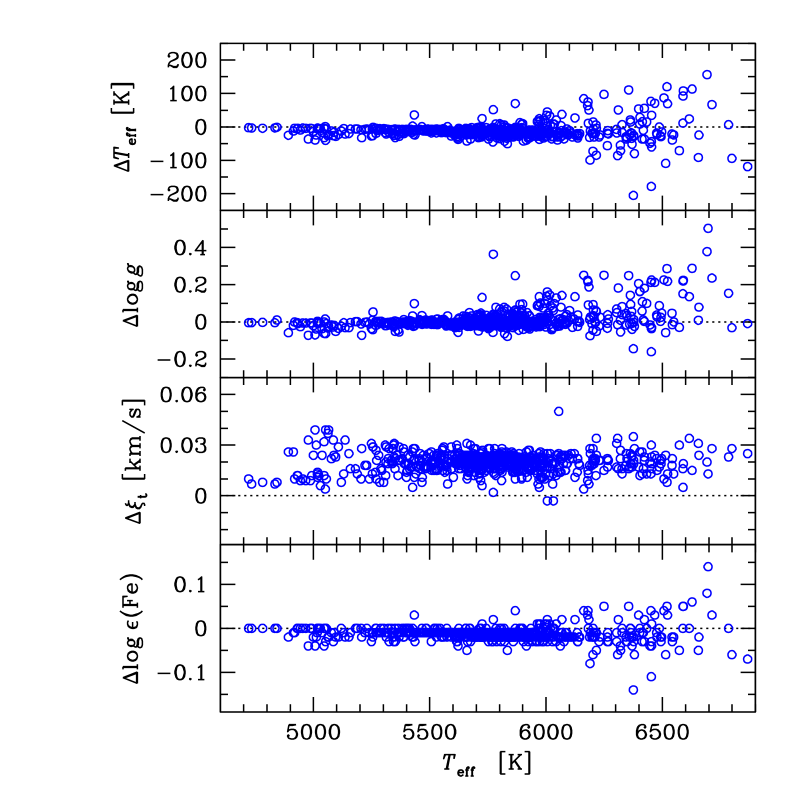
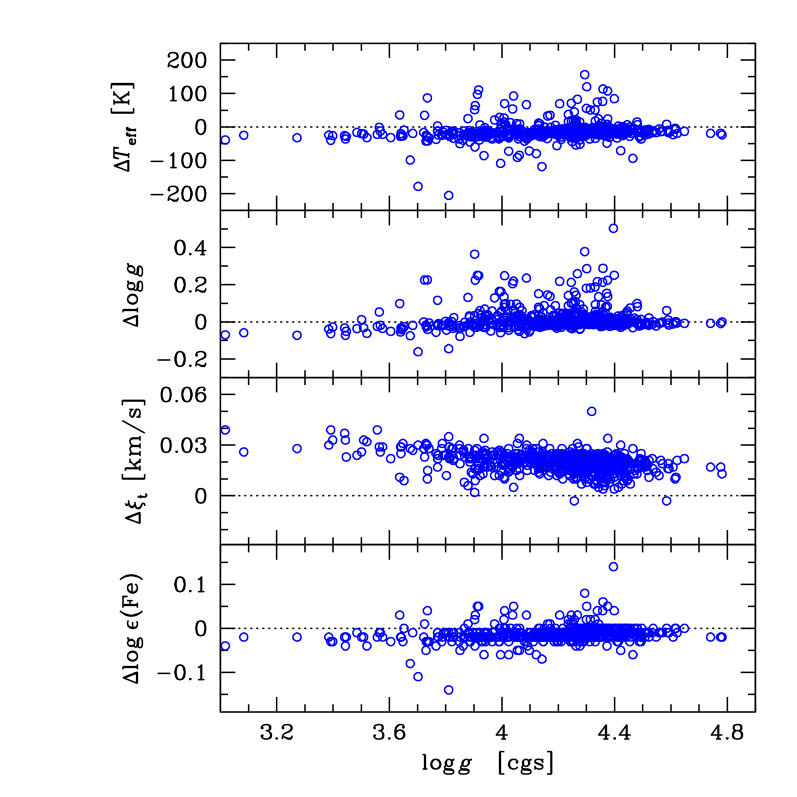
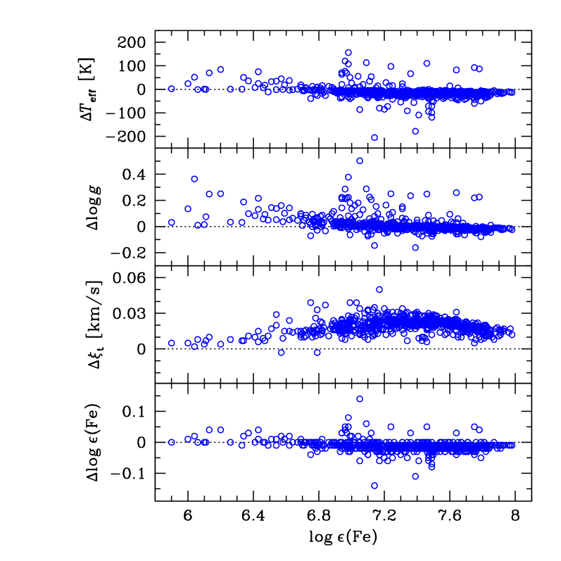
Stellar parameters were also determined without applying the Fe i NLTE corrections and Fig. 6 shows how the stellar parameters change. The differences are usually very small, but we do see a larger scatter in $T_{\rm eff}$, log $g$, and Fe abundance for stars with effective temperatures above approximately 6100 K. There might also be slight systematic trends with surface gravity, however, too small to be statistically significant.

The average effects on the stellar parameters are (NLTE values minus LTE values, and excluding stars with $T_{\rm eff}>6100$ K in parentheses): $\Delta T_{\rm eff}=-12\,(-14)\pm 28\,(12)$ K, $\Delta\log g=+0.012\,(+0.002)\pm 0.059\,(0.035)$, $\Delta\log\,({\rm Fe})=-0.013\,(-0.013)\pm 0.016\,(0.008)$, and $\Delta\xi_{\rm t}=+0.019\,(+0.020)\pm 0.006\,(0.006)$. For the Sun, the effect on the Fe abundance when applying the NLTE corrections is $-0.01$ dex. This means that for the whole sample of 714 stars the average metallicity becomes $-0.003$ dex lower after including the Fe i NLTE corrections in the analysis. While this is a truly minuscule effect, the effects on temperatures and surface gravities could have some impact on stellar ages, and possibly also when determining abundances for elements like Li, which is very temperature-sensitive. The stars for which we see significant effects are those that are warmer than about 6100 K.

Oxygen and sodium:

The oxygen abundances have been determined from the infrared triplet lines at 777 nm. These lines are known to be strongly affected by deviations from LTE (e.g., Kiselman 1993; Asplund et al. 2009). To correct our oxygen abundances for NLTE effects, we apply the empirical formula from Bensby et al. (2004b), who analysed the forbidden oxygen line at 630 nm, which is a very robust indicator of the oxygen abundance, unaffected by departures from LTE (e.g., Kiselman 1993; Asplund et al. 2009).

For sodium we applied the NLTE corrections from Lind et al. (2011), using an IDL script that was kindly provided by Karin Lind.

How the NLTE corrections affect the [O/Fe] and [Na/Fe] abundance ratios is shown in Fig. 7.

5.3 Surface gravity

Two widely used methods to determine the surface gravity are derived from ionisation balance between Fe i and Fe ii, and from basic principles through the relationship between bolometric flux, temperature, and gravity (see, e.g., Eq. 4 in Bensby et al. 2003). The latter requires that the distance to the star is known, and in our case all stars have distances based on Hipparcos parallaxes from the new reduction by van Leeuwen (2007).

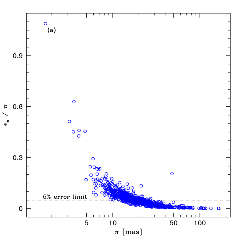
There are some indications that by using parallaxes to determine $\log g$ from basic principles, one introduces an external source of uncertainty, independent of the spectra. For instance, studies of solar analogs have shown that a purely spectroscopic approach (i.e. $T_{\rm eff}$ from excitation balance of abundances from Fe i lines and $\log g$ from ionisation balance of abundances from Fe i and Fe ii lines) has better precision than when using $\log g$ based on parallaxes (e.g., Ramírez et al. 2009). Another advantage of using a purely spectroscopic approach in our case is that the uncertainties will be essentially distance-independent. This is so because the sample contains relatively bright stars ($V<9$), and as a majority have been observed with large, 6-8 m class telescopes, the exposure times are short and the spectra have high signal-to-noise independent of the magnitude (or distance) of the star. If the parallax method is used, the uncertainties increase with distance, as is seen in Fig. 8, which shows the fractional parallax errors versus the parallaxes for our stars: there is a clear increase in the parallax error with distance. The sample contains 329 stars that have fractional errors in the parallax larger than 5 % and 89 stars larger the 10 %. Furthermore, for stars with large parallax uncertainties the Lutz-Kelker bias can be severe and is impossible to correct for on an individual basis.

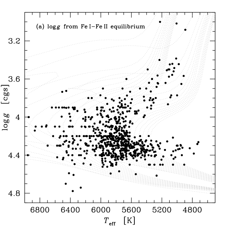
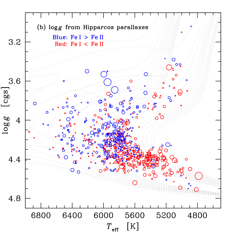
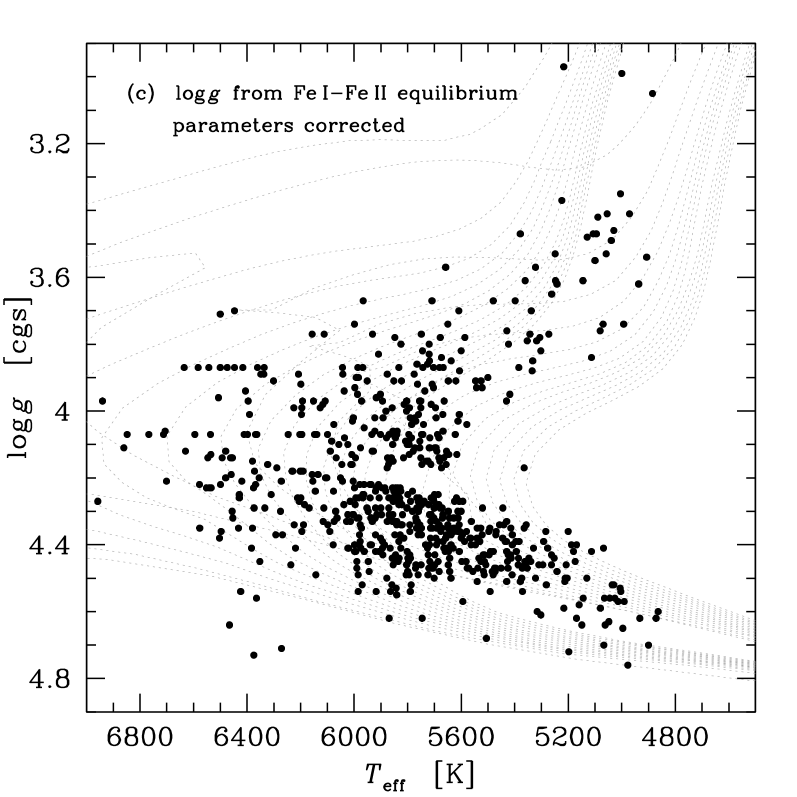
Therefore, we start by analysing our sample using ionisation balance to get the surface gravity. Figure 9a shows the resulting HR diagram, and at a first glance, it appears peculiar in the sense that the lower main sequence is horizontal rather than declining. As there are many stars that fall in regions unoccupied by isochrones, and as the whole appearance is somewhat “uncomfortable”, we redetermine the stellar parameters, but this time using the Hipparcos parallaxes to get the surface gravity. The resulting HR diagram, in Fig. 9b, having gravities based on Hipparcos parallaxes, shows a declining main sequence (as expected). It should be noted that the inclusion of the Fe i NLTE corrections are far too small to have an effect on the gravities of the magnitude to produce the flat lower main sequence.

Figure 10: The difference in abundances from Fe i and Fe ii lines versus effective temperature (a and b,), and versus surface gravity (c). Only stars with relative errors in their parallaxes smaller than 5 % are included, and the parameters are the ones when $\log g$ is determined from the Hipparcos parallax.

Figure 11: The difference in effective temperature (upper panels) and surface gravity (lower panels) from the ionisation balance and Hipparcos parallax methods for stars with a relative parallax uncertainty less than 5 %.

5.4 Investigating the flat lower main sequence

To further investigate the difference in the two methods for determining the surface gravity, the stars in Fig. 9b have been encoded in red if the resulting Fe i abundances are lower than the Fe ii abundances, and blue if the opposite is true. The sizes of the circles are scaled with the magnitude of the difference between Fe i and Fe ii abundances. What we see is that on the lower main sequence essentially all stars appear to be red, i.e. the Fe i abundances are lower than the Fe ii abundances. In other parts of the HR diagram, there is a mixture of red and blue circles. This is further illustrated in Fig. 10, where we plot the difference between Fe i and Fe ii abundances versus $T_{\rm eff}$ and $\log g$ for all stars that have relative parallax uncertainties less than 5 %. The stars above the turn-off ($\log g<4.2$) show perfectly flat trends with both $T_{\rm eff}$ and $\log g$, while many stars below the turn-off with $T_{\rm eff}\lesssim 5600$ K show large discrepancies between Fe i and Fe ii. There is also a declining trend in Fe i–Fe ii with $\log g$ that also increases in dispersion with $\log g$. In summary, it appears that essentially all stars with $\log g>4.2$ and $T_{\rm eff}<5650$ do not show ionisation equilibrium between Fe i and Fe ii when determining the surface gravity from Hipparcos parallaxes.

Figure 12: HR diagrams for the Reddy et al. (2003, 2006) sample, the Valenti & Fischer (2005) sample, and the Adibekyan et al. (2012) sample. Overlapping stars from this study are marked by red solid circles. The $\alpha$-enhanced Yonsei-Yale (Y2) isochrones by Demarque et al. (2004) have metallicities of $\rm[Fe/H]=-1$ and $+0.3$ dex, respectively, and are shown from 1 to 15 Gyr in steps of 1 Gyr.

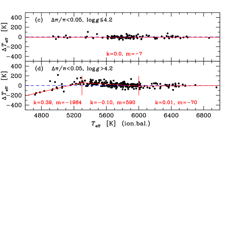
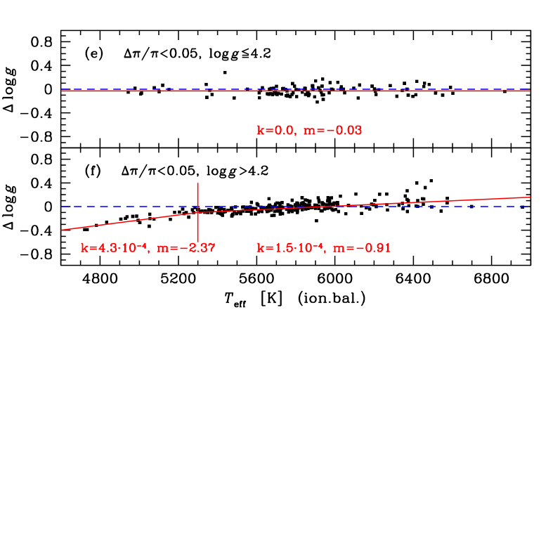
The question is now which method to use to get a consistent analysis. As a significant fraction of the stars in the sample have parallax uncertainties larger than 5 % (see Fig. 8), the best way would be to use ionisation balance. Ionisation balance also has a large advantage over the parallax method as it is based on the stellar spectrum only, and can be utilised even when the distance to the star is not known to high precision, such as in the case of microlensed dwarf stars in the Galactic bulge. On the other hand, from the analysis of nearby stars with very good Hipparcos parallaxes, it is evident that ionisation balance has its limitations, and mainly on the lower main sequence for stars with $\log g\gtrsim 4.2$ and $T_{\rm eff}\lesssim 5600$ K. Figures 11a and b shows the differences between the effective temperatures and surface gravities that the two methods generate as a function of the surface gravity. For $\log g\lesssim 4.2$ there appears to be a slight constant offset, while for higher $\log g$ there might be a rising trend, although it is difficult to say as the dispersion also increases. The differences as a function of effective temperature shown in Figs. 11c-f have a clearer appearance. The sample is split at $\log g=4.2$, which is roughly in the turn-off region. For stars above the turn-off ($\log g\lesssim 4.2$) there appears to be a constant small offset in both $T_{\rm eff}$ and $\log g$; $-7$ K and $-0.03$ dex, respectively. Below the turn-off the situation appears more complicated and we make linear regressions to the regions defined in Figs. 11d and f. The corrections $\Delta T$ and $\Delta G$ to be applied (subtracted) to the ionisation balance parameters are given in Table 2.

Table 2: Corrections to be applied to the parameters from ionisation balance. $T_{\rm eff}(corr)=T_{\rm eff}-\Delta T$ and $\log g(corr)=\log g-\Delta G$ where $\Delta T=k_{T}*T_{\rm eff}+m_{T}$ and $\Delta G=k_{G}*T_{\rm eff}+m_{G}$ with the parameters given in the table below. Relationships are illustrated in Figs. 11c-f.

$T_{\rm eff}$ interval	$\log g$ interval	$k_{T}$	$m_{T}$	$k_{G}$	$m_{G}$
$4600-7000$	$3.0-4.2$	0.00	$-$7	0.00	-0.03
$4600-5300$	$4.2-4.8$	0.39	$-$1984	$4.3\cdot 10^{-4}$	$-$2.4
$5300-6000$	$4.2-4.8$	$-$0.11	590	$1.5\cdot 10^{-4}$	$-$0.91
$6000-7000$	$4.2-4.8$	0.025	$-$70	$1.5\cdot 10^{-4}$	$-$0.91

The HR diagram based on the corrected ionisation balance parameters is shown in Fig. 9c. The gap that can be seen at $\log g\approx 4.2$ is an artefact due to that the corrections are different for stars below and above the turn-off.

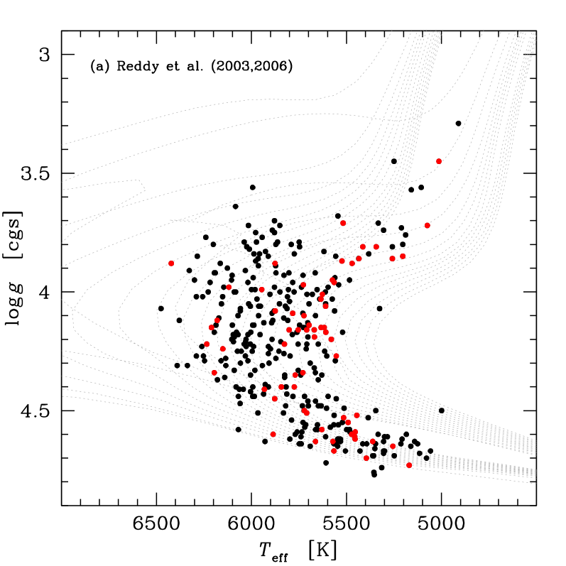
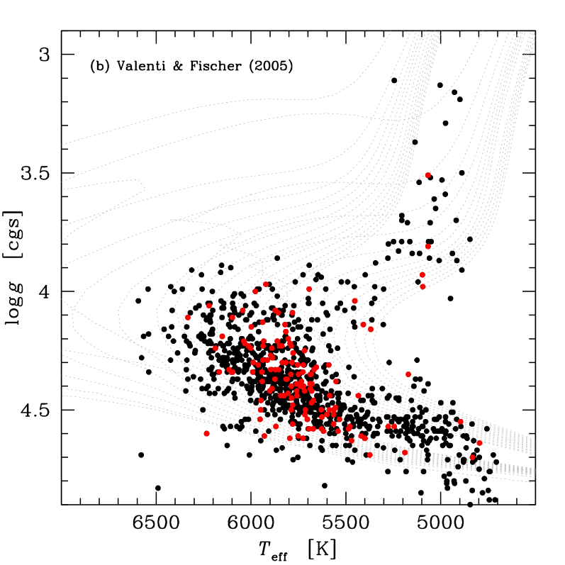
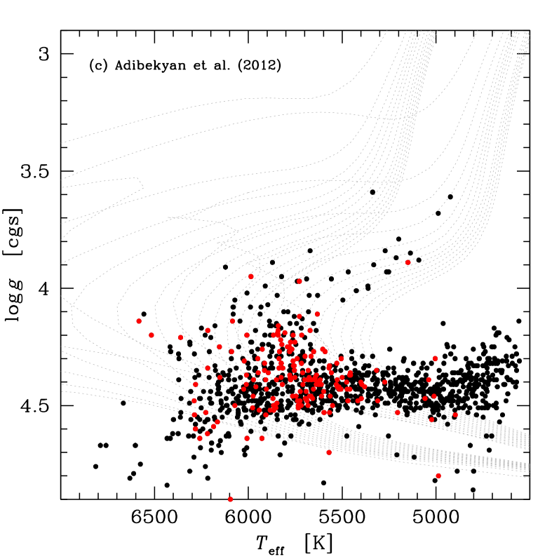
After having identified these ionisation balance issues on the lower main sequence for our sample, it is interesting to see whether flat main sequences are present in other similar high-resolution spectroscopic studies of the Galactic disk. For that, we choose three studies: first, the sample of 355 dwarf stars from Reddy et al. (2003, 2006) where stellar parameters are determined from the infrared IRFM flux method and Hipparcos parallaxes; second, the sample of 1040 dwarf stars from Valenti & Fischer (2005) where stellar parameters are determined through $\chi^{2}$-minimisation between observed spectrum and synthesised spectrum in selected wavelength bands using the SME software; and third, the sample of 1111 dwarf stars from Adibekyan et al. (2012) who, like us, use ionisation and excitation balance to determine stellar parameters. The HR diagrams for these studies are shown in Fig. 12. For the Reddy et al. (2003, 2006) and Valenti & Fischer (2005) studies, which do not utilise ionisation balance, the HR diagrams appear normal, with declining main sequences. The HR diagram for the Adibekyan et al. (2012) sample, on the other hand, shows an extremely flat relation, where $\log g$ is even slightly rising with decreasing temperature.

What the causes are for the flat main sequence is not all clear. It is possible that they arise due to limitations of the models that cannot properly handle excitation balance and/or ionisation balance. Or it could be that NLTE effects and/or 3D effects play roles, or a combination of all of these. It is beyond the scope of the current paper to further investigate this, and we will for now settle with the empirical corrections in Table 2. We will report stellar parameters for all three varieties (ionisation balance, parallaxes, corrected ionisation balance), but elemental abundances and stellar ages will only be reported for the corrected ionisation balance values, which is also what will be used in the remainder of the paper. All parameters are reported in Table 7.

5.5 Systematic errors

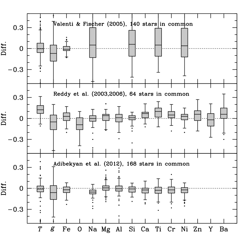
As the analysis is strictly differential relative to the Sun, systematic errors should largely cancel out and the internal precision should be good. This is seen through the good agreement between equivalent width measurements and stellar parameters that we derive for the Sun based on the spectra from the different spectrographs and observing runs. Systematic shifts relative to other studies are more difficult, as methods, model atmospheres, atomic data, and methods for normalisation to the Sun, might differ. To check and compare our results we have made a detailed comparison of our stellar parameters and elemental abundances to three recent and large studies of the Galactic stellar disk. First we have chosen the studies by Reddy et al. (2003, 2006), consisting of stars observed from the Northern hemisphere at the MacDonald Observatory. In total this sample consists of 355 kinematically selected F and G dwarf stars that nicely would complement our sample, which mainly has been observed from the Southern hemisphere. With Reddy et al. (2003, 2006) we have 64 stars in common. Next, we have chosen the study by Adibekyan et al. (2012) who have done a detailed abundance analysis of 1111 stars observed with the HARPS spectrograph on the ESO 3.6-m telescope on La Silla. With Adibekyan et al. (2012) we have 168 stars in common. And finally, we have chosen the Valenti & Fischer (2005) study of 1040 F, G, and K dwarfs from the Keck, Lick, and AAT planet search programs, with which we have 140 stars in common. The stars in common with each of these studies are marked in red in the HR diagrams in Fig. 12.

Figure 13: Comparison of abundances ($[X/{\rm H}]$) for stars in common between this study and those of Valenti & Fischer (2005), Reddy et al. (2003, 2006), and Adibekyan et al. (2012). The elements ($X$) are indicated on the abscissa. The two left-most boxes in each panel show the $T_{\rm eff}$ (denoted by $T$) and $\log g$ (denoted by $g$) comparisons. Please note that the scale on the ordinate for the temperature should be multiplied by a factor 100. The differences are given as our values minus their values, and the differences are also listed in Table 3. In the boxplots the central horizontal line represents the median value. The lower and upper quartiles are represented by the outer edges of the boxes, i.e., the box encloses 50 % of the sample. The whiskers extend to the farthest data point that lies within 1.5 times the inter-quartile distance. Those stars that do not fall within the reach of the whiskers are regarded as outliers and are marked by dots.

Table 3: Comparisons of stars in common with Reddy et al. (2003, 2006), Adibekyan et al. (2012), and Valenti & Fischer (2005). The differences are given as values from this work minus the other studies. The values given are the median value as well as the 1-$\sigma$ dispersion around the median.

	R03/06	A12	VF05
# of stars	355	1111	1040
overlap	64	168	140
$\Delta T_{\rm eff}$	$+124\pm 57$	$-10\pm 42$	$-2\pm 67$
$\Delta\log g$	$-0.05\pm 0.10$	$-0.06\pm 0.10$	$-0.07\pm 0.12$
$\rm\Delta[Fe/H]$	$+0.03\pm 0.05$	$-0.02\pm 0.04$	$-0.01\pm 0.03$
$\rm\Delta[O/H]$	$-0.09\pm 0.08$
$\rm\Delta[Na/H]$	0$0.00\pm 0.04$	$-0.05\pm 0.03$	$+0.05\pm 0.21$
$\rm\Delta[Mg/H]$	$+0.04\pm 0.04$	$+0.01\pm 0.03$
$\rm\Delta[Al/H]$	$+0.01\pm 0.05$	$-0.01\pm 0.04$
$\rm\Delta[Si/H]$	$+0.01\pm 0.03$	$-0.01\pm 0.04$	$+0.06\pm 0.18$
$\rm\Delta[Ca/H]$	$+0.07\pm 0.04$	$-0.02\pm 0.03$
$\rm\Delta[Ti/H]$	$+0.10\pm 0.06$	$-0.03\pm 0.04$	$+0.05\pm 0.20$
$\rm\Delta[Cr/H]$	$+0.05\pm 0.04$	$-0.02\pm 0.04$
$\rm\Delta[Ni/H]$	$+0.03\pm 0.04$	$-0.02\pm 0.04$	$+0.04\pm 0.20$
$\rm\Delta[Zn/H]$	$+0.06\pm 0.07$
$\rm\Delta[Y/H]$	$-0.02\pm 0.09$
$\rm\Delta[Ba/H]$	$+0.06\pm 0.07$

Figure 13 and Table 3 show the comparisons to the Reddy et al. (2003, 2006), Adibekyan et al. (2012), and Valenti & Fischer (2005) studies. The comparisons are very favourable and we see that our results compare reasonably well. With a few exceptions, the median difference in the abundance ratios are well below 0.1 dex. The main difference lies in the comparison of the Na, Si, Ti, and Ni abundances from Valenti & Fischer (2005) where the dispersion is much larger than in the comparisons to Reddy et al. (2003, 2006) and Adibekyan et al. (2012). Note that most stars in common with Adibekyan et al. (2012) are located in the turn-off region and not on the lower main sequence (see Fig. 12), so systematics due to the flat main sequence issue should not be significant.

5.6 Random errors

An error analysis, as outlined in Epstein et al. (2010), has been performed for all stars. The method accounts for abundance spreads (line-to-line scatter) as well as how the abundances for each element react to changes in the stellar parameters. The details of the method are given in Appendix B.

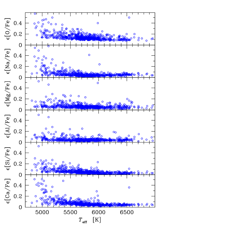
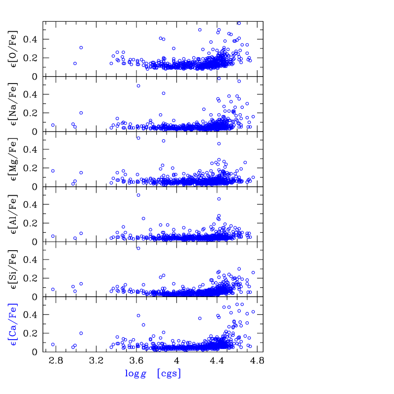
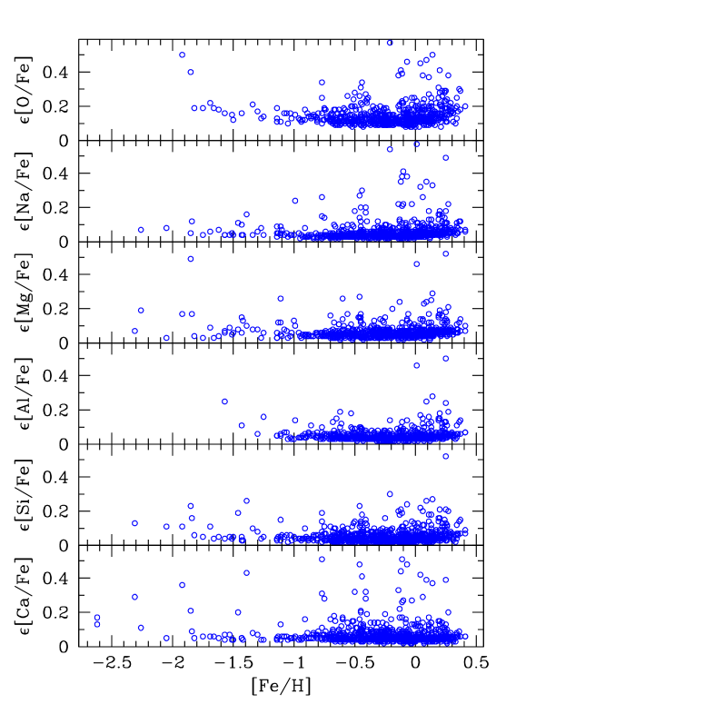
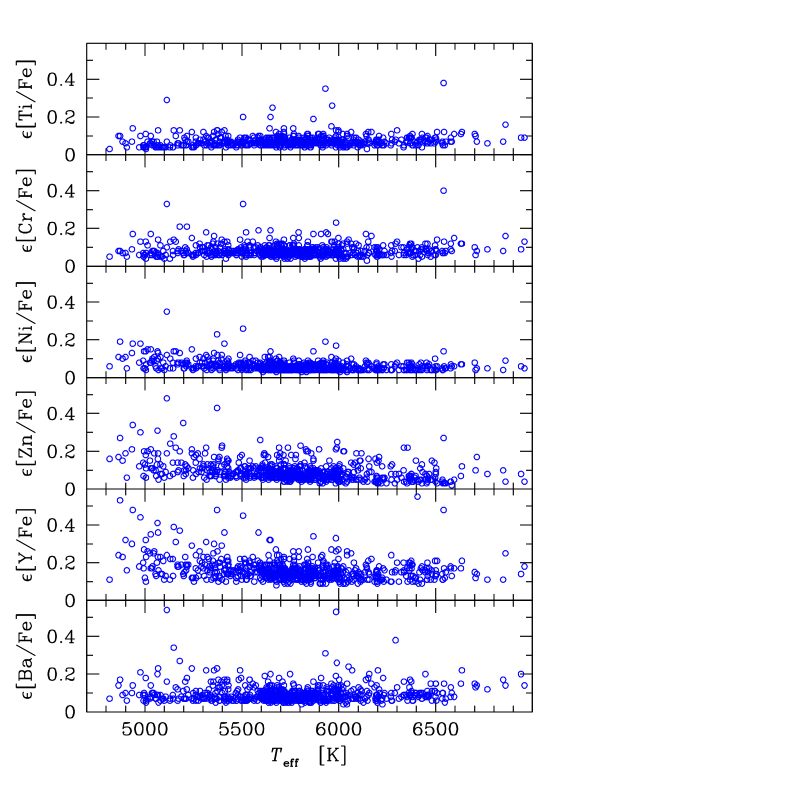
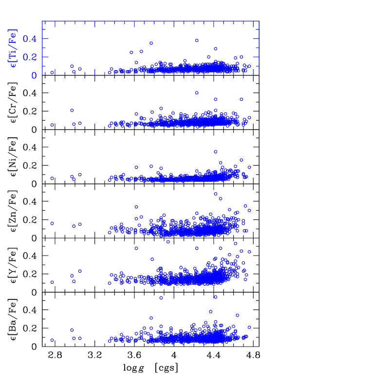
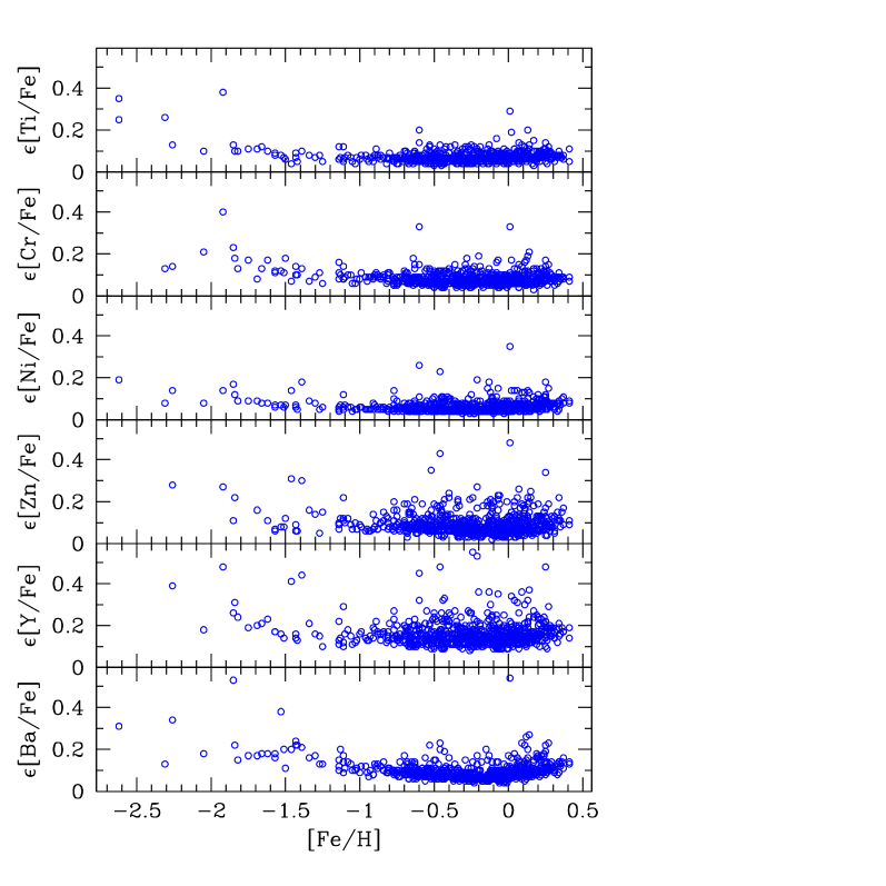
Figure 14 shows the uncertainties for the stellar parameters and the abundance ratios as a function of temperature, gravity, and metallicity. The uncertainties are reasonably small and it is only for low effective temperatures (below about 5400 K), higher gravities, and at the highest [Fe/H] where they start to become substantial. Interestingly, contrary to the other $\alpha$-elements, the uncertainty in [Ti/Fe] stays low and flat for essentially all parameters. In the upcoming sections (from Sect. 6.3 and onwards) where we investigate different properties of the Galactic disk we will therefore mainly utilise the Ti results.

Uncertainties in the stellar parameters and in the abundance ratios ([$X$/Fe] and [$X$/Ti]) are given in Table 7.

Figure 14: Uncertainties in stellar parameters and abundance ratios as a function of $T_{\rm eff}$, $\log g$, and [Fe/H].

Figure 15: [$X$/Fe] versus [Fe/H] plots for the $\alpha$-elements (O, Mg, Si, Ca and Ti) and the light element Al. The full sample of 714 stars is shown and black dots show the 604 stars with $T_{\rm eff}>5400$ K and grey dots the stars with $T_{\rm eff}<5400$ K. A typical error bar is shown in each plot.

Figure 16: [$X$/Fe] versus [Fe/H] plots for the light element Na, the iron-peak elements Cr, Ni, and Zn, and the s-process elements Y and Ba. The full sample of 714 stars is shown and black dots show the 604 stars with $T_{\rm eff}>5400$ K and grey dots the stars with $T_{\rm eff}<5400$ K. For Ba, stars with $T_{\rm eff}>6100$ K have been identified by red circles. A typical error bar is shown in each plot.

5.7 Age determination

Stellar ages were determined from a fine grid of $\alpha$-enhanced Yonsei-Yale (Y2) isochrones by Demarque et al. (2004), adopting $\rm[\alpha/Fe]=0$ for $\rm[Fe/H]>0$, $\rm[\alpha/Fe]=-0.3\times[Fe/H$] for $\rm-1\leq[Fe/H]\leq 0$, and $\rm[\alpha/Fe]=+0.3$ for $\rm[Fe/H]<-1$. Taking the errors in effective temperature, surface gravity, and metallicity into account, an age probability distribution (APD) was constructed for each star. The most likely age, as well as lower and upper age estimates, was estimated from this APD as described in Meléndez et al. (2012) and a short outline in Bensby et al. (2011a). In a similar manner, stellar masses were determined as well. Ages, masses, and their associated uncertainties are given in Table 7.

6 Elemental abundance results

Studies of elemental abundances in nearby stars are important. Gratton et al. (2000) showed that stars on cold disk orbits have lower [$\alpha$/Fe] than stars that move on halo and thick disk-like orbits. Fuhrmann (1998, 2000, 2004, 2008, 2011) showed that stars very close to the Sun trace two distinct abundance trends. Several recent studies have obtained elemental abundances for stars that have typical thin and thick disk kinematics; these also show distinct trends (e.g., Bensby et al. 2003, 2005, 2007b; Reddy et al. 2003, 2006; Adibekyan et al. 2012). However, recently there has been quite some debate about whether the Milky Way has a distinct thick disk or whether it forms a continuum with the thin disk (see, e.g., Bovy et al. 2012).

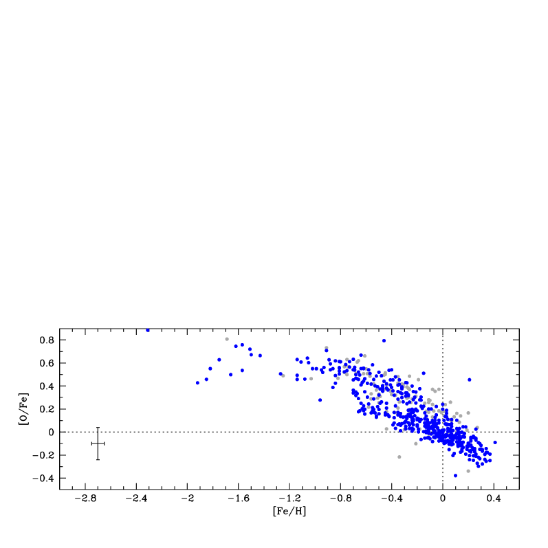
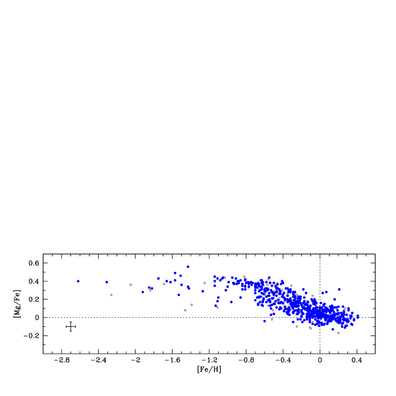
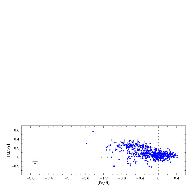
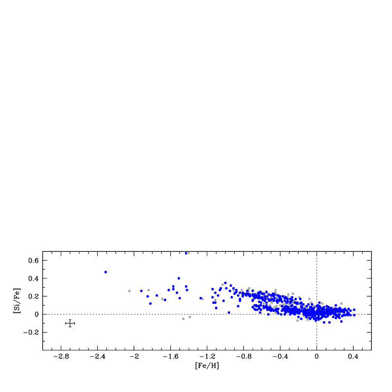
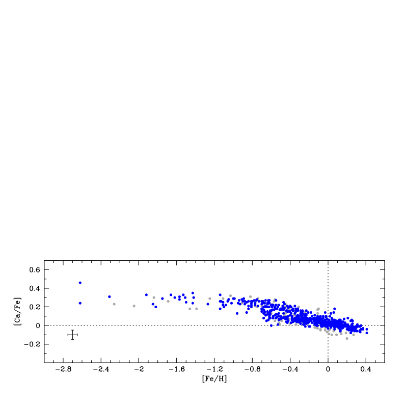
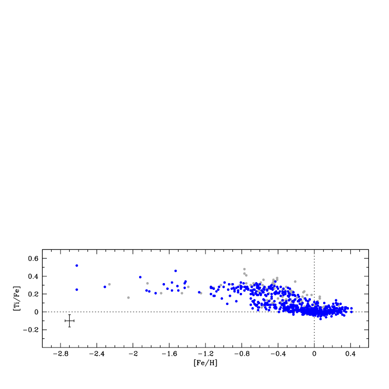
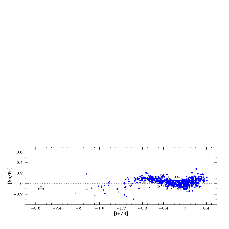
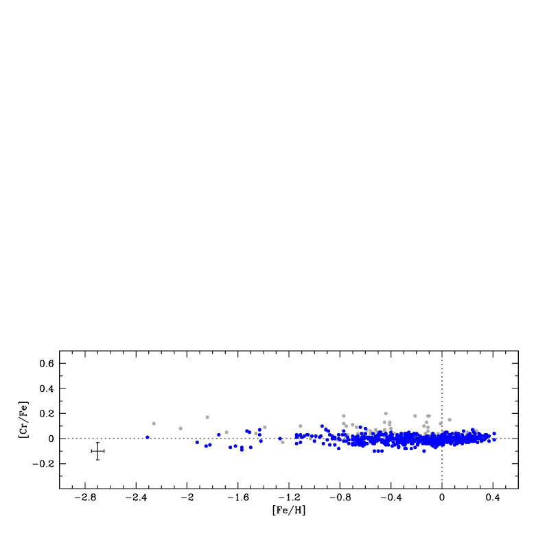
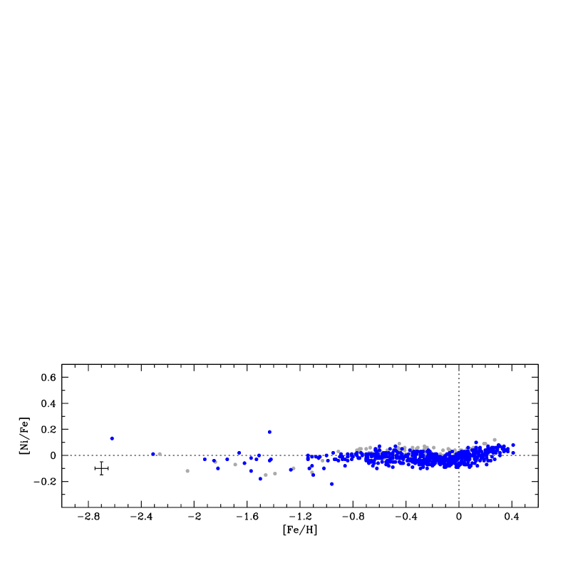
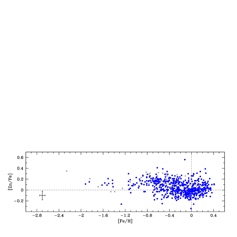
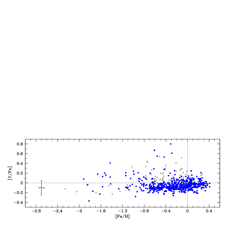
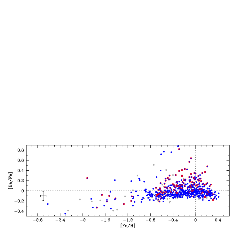
Figures 15 and 16 show the resulting abundance trends for the full sample of 714 stars. In Sect. 5.6 we saw that the uncertainties tend to increase for stars at lower temperatures and higher surface gravities. By restricting the sample to those stars with $T_{\rm eff}>5400$ K many of the stars with high uncertainties will be avoided. 604 of the 714 stars in the sample have $T_{\rm eff}>5400$ K. In the abundance plots in Figs. 15 and 16 we have therefore marked the stars that have temperatures lower than 5400 K by grey dots.

The abundance plots for oxygen, Mg, Si, Ca, and Ti show a flat plateau in [$X$/Fe] for stars more metal-poor than $\rm[Fe/H]\lesssim-0.5$. At higher [Fe/H] there is a general downward trend. From $\rm[Fe/H]\approx-0.7$ and upwards, there appears to be two abundance trends. At super-solar metallicities [O/Fe], and possibly also [Ca/Fe] and [Mg/Fe] show downward trends with [Fe/H], while the [Si/Fe] and [Ti/Fe] trends are practically flat.

Na and Al are light odd-Z elements and we see that Al behaves like an $\alpha$-element, showing all the characteristics that the genuine $\alpha$-elements do, i.e., a flat plateau at lower [Fe/H] that at higher [Fe/H] starts to decline toward solar values. The [Na/Fe] trend shows less dispersion than [Al/Fe] and there is no resemblance with Al or the $\alpha$-elements. Instead [Na/Fe] is almost solar, with a slightly curved appearance, that rises at super-solar [Fe/H].

Figure 17: Generalised abundance ratio histograms for the O, Mg, Si, Ca, and Ti for stars in the interval $\rm-0.7<[Fe/H]<-0.35$. Shaded histograms show stars with $T_{\rm eff}>5400$ K. The red dash-dotted lines show the fraction of rejected stars when selecting stars with $T_{\rm eff}<5400$ K.

Both [Ni/Fe] and [Cr/Fe] show internally extremely small dispersions and vary essentially in lock-step with [Fe/H]. The only discernible pattern is that the [Ni/Fe] ratio is slightly below solar values at $\rm[Fe/H]<0$ and that it then shows a shallow increase at $\rm[Fe/H]>0$. The latter feature turns out to be an important feature when determining oxygen abundances from the forbidden [Oi] line at 6300Å̇ which is blended with Ni i lines (see Bensby et al. 2004b). We note that the few stars in the [Cr/Fe] plot that lie slightly above the very flat trend of the bulk of stars are all stars that fall outside the selected temperature interval (grey coloured).

Zn is the second even-Z element beyond the iron-peak and albeit with a scatter, we find a somewhat declining [Zn/Fe] trend with metallicity, from being slightly elevated at $\rm[Fe/H]\lesssim-0.5$, to being solar at $\rm[Fe/H]\gtrsim 0$. There is also a slight resemblance with the $\alpha$-elements. At lower metallicities $\rm[Fe/H]<-1$, $\rm[Zn/Fe]$ is roughly constant at $\approx 0.1$, meaning that Zn could serve as a good proxy for Fe in metal-poor damped Lyman alpha systems as it can be observed in damped Lyman alpha systems without being depleted by interstellar/galactic dust (e.g., Kobayashi et al. 2006)).

Both Y and Ba are $s$-process elements and we see that are slightly under-abundant relative to Fe. We note that most of the stars in the [Ba/Fe] plot that have high Ba abundances around solar [Fe/H] disappear when discarding stars with $\rm T_{\rm eff}<5400$ temperature range. The same is also true for [Y/Fe]. Furthermore, Ba is known to suffer from NLTE effects at higher $T_{\rm eff}$ (e.g., Korotin et al. 2011) and stars in the [Ba/Fe] plot with $T_{\rm eff}>6100$ K have therefore been marked with red circles. We see that essentially all stars with high [Ba/Fe] around solar metallicities also have high temperatures.

Figure 18: Boxplots showing the distribution of abundance ratios for 16 stars with $T_{\rm eff}>5400$ K and an upper age limit of 7 Gyr, in a narrow metallicity range around that of the Sun ($\pm 0.03$ dex). Due to large NLTE effects for Ba at higher temperatures, the Ba box has been further restricted to $T_{\rm eff}<6000$ K. In the boxplots the central horizontal line represents the median value. The lower and upper quartiles are represented by the outer edges of the boxes, i.e., the box encloses 50 % of the sample. The whiskers extend to the farthest data point that lies within 1.5 times the inter-quartile distance. Those stars that do not fall within the reach of the whiskers are regarded as outliers and are marked by dots.

6.1 The [$\alpha$/Fe] distribution at intermediate [Fe/H]

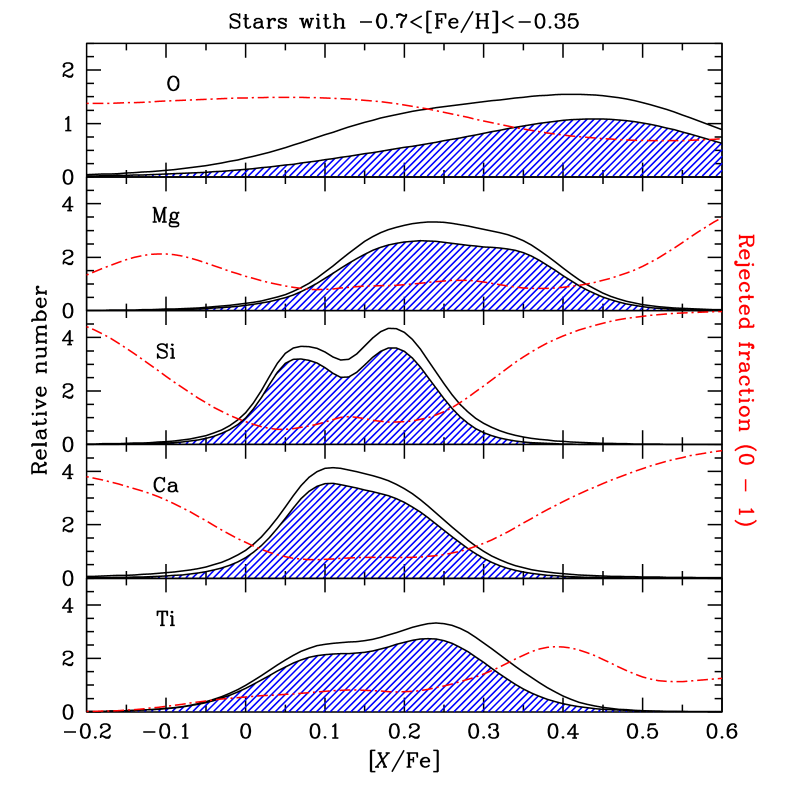
The region where the potential gap, or bimodality, between the thin and thick disk abundance trends is largest is for metallicities in the interval $-0.7\lesssim\rm[Fe/H]\lesssim-0.35$. Due to observational uncertainties and the magnitude of the astrophysical signature, this gap appears clear for some elements and less so for others. From the abundance trend plots in Figs. 15 and 16, it is evident that the scatter decrease and that the abundance trends become more well-defined when only including stars with $T_{\rm eff}>5400$ K. To further highlight the effects, Fig. 17 shows the generalised [$X$/Fe] histograms for O, Mg, Si, Ca, and Ti for stars in the metallicity range $\rm-0.7<[Fe/H]<-0.35$. The empty and shaded histograms show the distributions when including or discarding the stars with $T_{\rm eff}<5400$ K, respectively. The red dash-dotted lines show the fraction of the sample as a function of $[X/{\rm Fe}]$ that gets rejected when selecting stars with $T_{\rm eff}<5400$ K . Especially for Si, and perhaps Mg and Ti, one sees that a higher fraction of the “bad” stars with $T_{\rm eff}<5400$ K are located in the gap area and that the potential bimodality becomes clearer when discarding the stars that are more prone to uncertainties. For all abundance trends there is a large fraction of “bad” stars at the lower and upper limits of the abundance ratios, i.e., these stars increase the dispersion in the plots. This demonstrates that uncertainties potentially can wash out differences between stellar populations (see also Lindegren & Feltzing 2013, for a quantitative analysis).

6.2 The abundance pattern of the Sun

Several studies give opposing results regarding the Sun’s abundance pattern relative to what is seen for the Galactic disk (e.g., Meléndez et al. 2009; Ramírez et al. 2010). In Fig. 18 we show the abundance ratios for young disk stars in a narrow metallicity range around that of the Sun ($\pm 0.05$ dex) that have upper age estimates below 7 Gyr, and discarding stars that are more susceptible to uncertainties (i.e. only keeping stars with $T_{\rm eff}>5400$ K, see 5.6). For most of the abundance ratios the Sun appears to be “normal”, i.e., the lines showing the median values in the boxplots are close to zero. For the few abundance ratios where the central 50 % fall either above or below a value of zero, the median line is still within 0.05 dex of the Sun. Based on this, the Sun appears not to be too different from the bulk of young disk stars in the immediate Solar neighbourhood.

6.3 Statistical definitions of stellar populations based on kinematics

Many recent studies of the stellar disk in the Milky Way have aimed to characterise the elemental abundances for stars that are thought to belong to the thick and thin disks. It thus became important to select stars that likely belong, respectively, to the two disks. An expedient way to do this is to use kinematical criteria such as the one from Bensby et al. (2003, 2005), and which is outlined in Appendix A.

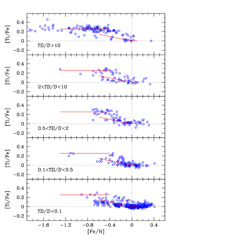
Figure 19 shows the [Ti/Fe]-[Fe/H] abundance trends for five different cuts in the thick disk-to-thin disk probability ratios $(TD/D)$ that indicate how much more likely it is that a star belongs to the thick disk than the thin disk. The top panel shows the stars that are at least ten times more likely to be thick disk stars, while the bottom panel shows stars that are at least ten times more likely to be thin disk stars. The three panels in the middle show probabilities in between, with the middle one containing stars that cannot easily be classified as either thin disk or thick disk. What we see is that even with these very extreme definitions of the samples there is a significant overlap in the sense that there are stars with either classification that fall on the abundance trend normally associated with the other population (see also, e.g., Fuhrmann 1998; Bensby et al. 2003; Reddy et al. 2006). This is an obvious consequence of this kinematical classification, as stars from the low-velocity tail of the thick disk will be classified as thin disk stars, while stars from the high-velocity tail of the thin disk will be classified as thick disk stars (assuming that there are two distinct trends for the elemental abundances).

Figure 19: [Ti/Fe] as a function of [Fe/H] selected on $TD/D$ as indicated in each panel for stars with $T_{\rm eff}>5400$ K. To guide the eye, the red lines outline the thick disk abundance plateau and the decrease in the thin disk abundance ratio, respectively.

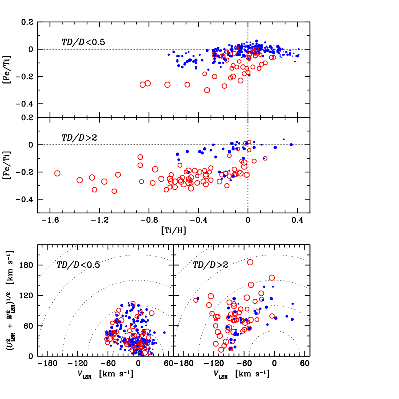
To further investigate the mixing of populations when using kinematical selection criteria we show in the upper panel on the left-hand side of Fig. 20 the [Fe/Ti]-[Ti/H] abundance trends for two kinematically selected samples: one where the probabilities of being a thin disk star are at least twice that of being a thin disk star $(i.e.,TD/D<0.5)$; and one where the probabilities of being a thick disk star are at least twice that of being a thick disk star $(i.e.,TD/D>2)$. This time we have coded the sizes of the markers by the ages of the stars and include only stars with good age estimates ($\rm\Delta Age<4$ Gyr). It is evident that the “second”, weaker, abundance signature in each sample has the same age structure as the main signature in the other sample. The Toomre diagrams for the two subsamples in the bottom panel on the left-hand side of Fig. 20 shows that the two samples are kinematically very different, with little overlap. Hence, it is apparent that there are kinematically cold stars that are old and $\alpha$-enhanced, as well as kinematically hot stars that are young and less $\alpha$-enhanced.

Figure 20: Left-hand side plots show the [Fe/Ti] versus [Ti/H] abundance trends when using the kinematical criteria as defined in Bensby et al. (2003, 2005). Stars have been colour- and size-coded depending on their ages. Right-hand side plots shows the abundance trends when splitting the sample according to their ages (as indicated). For all plots we have only included stars whose ages have been better determined than 4 Gyr (difference between upper and lower age estimates).

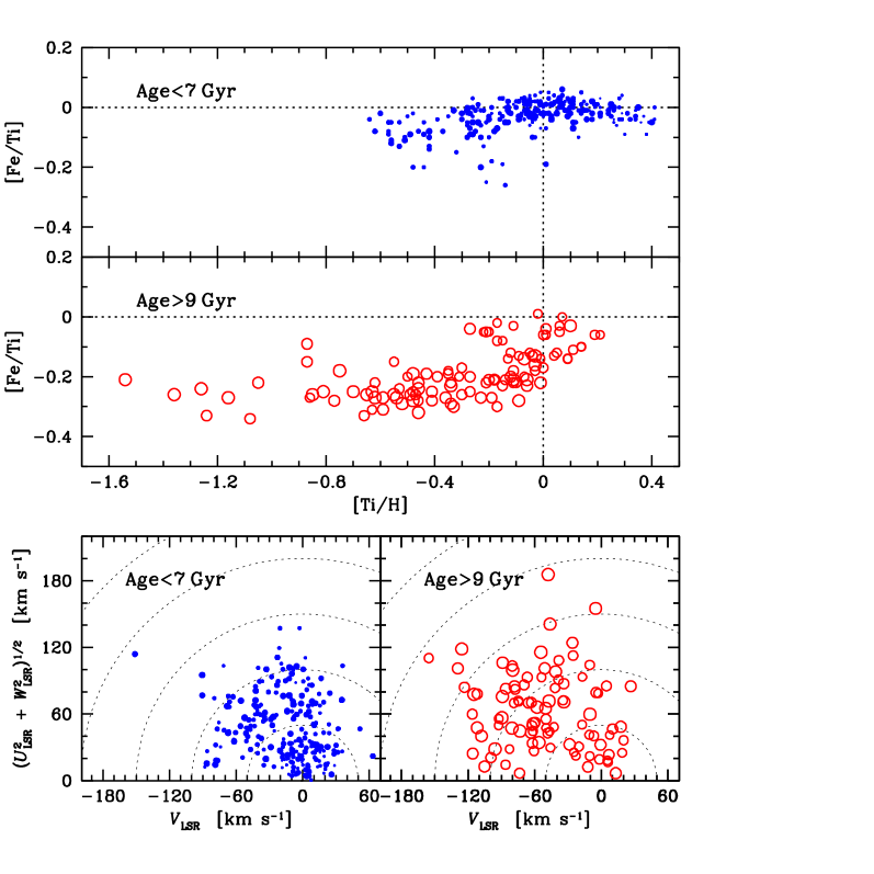
What about stellar age? Could this be a better discriminator between the thin and thick disks? The [Fe/Ti]-[Ti/H] abundance trends for two samples, one old sample with stars that have estimated ages greater than 9 Gyr, and one young sample with stars that have estimated age less than 7 Gyr, are shown in the upper part on the right-hand side of Fig. 20. Once again we see two very different chemical signatures, similar to the ones on the left-hand-side when the selection of the samples was based on kinematics. However, the difference is now that the two abundance trends are somewhat “cleaner”, with less “mirroring” between them. Looking at the Toomre diagrams for these two age-selected subsamples (bottom panel on the right-hand side of Fig. 20), there is a large kinematical overlap, i.e. there are many young stars with hot kinematics and many old stars with cold kinematics.

In summary, we note that there appears to be no perfect way of selecting thin and thick disk stars. While velocities and distances can be pinpointed to rather high accuracies there seem to be a large kinematical overlap between the two populations. Ages on the other hand appear to be better, but as good ages are notoriously difficult to obtain, there is also a significant overlap (due to the errors). However, it appears as if stellar ages might be a somewhat better discriminator when selecting thin and thick disk stars from nearby stellar samples. In kinematically selected thin disk samples we are prone to be contaminated by the low-velocity tail of the thick disk, and especially so at lower metallicities, and for kinematically selected thick disk samples we are prone to be contaminated by the high-velocity tail of the thin disk, and especially so at higher metallicities.

7 Discussions

7.1 Ages and metallicities

7.1.1 Old and metal-rich stars?

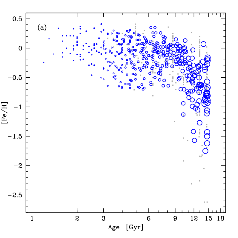
Recent high-resolution spectroscopic studies indicate that most stars with thick disk kinematics are older than those with thin disk kinematics (e.g., Gratton et al. 2000; Feltzing & Gonzalez 2001; Bensby et al. 2005). However, considerably larger samples available in photometric studies such as the GCS indicate the existence of a significant number of stars with thin disk kinematics that have high ages ($>10$ Gyr). Figure 21a shows the age-metallicity relation for our sample, and we also see that our sample possibly contains such old and metal-rich stars. However, the stars that have ages greater than 10 Gyr and metallicities higher than solar, all have large uncertainties (red small dots in Fig. 21). Hence, the parameters for these stars are doubtful and cast doubt on the existence of (very) old and metal-rich (super-solar) stars.

7.1.2 Age-metallicity relations?

In Bensby et al. (2004a) we investigated whether stars with kinematics typical for the thick disk showed any signs of an age-metallicity relation. We found, in accordance with other studies (e.g., Haywood 2006; Schuster et al. 2006), that stars with kinematics typical of the thick disk show an age-metallicity relation such that more metal-rich stars on average are younger than the less metal-poor stars in the sample. The stars older than about 8 Gyr in Fig. 21a show a trend of declining metallicity with age, consistent with the age-metallicity relation seen for thick disk stars in the studies mentioned above. Younger stars do not show this behaviour. Instead there appears to be a rather large scatter in age over the whole metallicity range ($-$0.8 to +0.4 dex), i.e., no apparent age-metallicity relation.

7.1.3 [$\alpha$/Fe] as a proxy for age?

Figure 21: Age-metallicity relation for those stars that have an age difference between upper and lower estimate of less than 4 Gyr. The sizes of the circles have been scaled with the ages of the stars. Stars with larger age uncertainties are shown as small grey dots.

Recently, Navarro et al. (2011) have argued that it is better to identify stars with different populations based on their elemental abundances rather than other properties such as kinematics. That a statistical selection based on kinematics causes overlaps between various abundance trends is evident from the nature of that selection process (see Sect. 6.3), and casts doubt on the reality of distinct trends for different stellar populations. This argument was used, e.g., by Bovy et al. (2012) when they investigated the scale-height of mono-abundance populations (i.e., stars that fall in a narrow range of elemental abundances, e.g., [$\alpha$/Fe] and [Fe/H]) in the SEGUE data set.

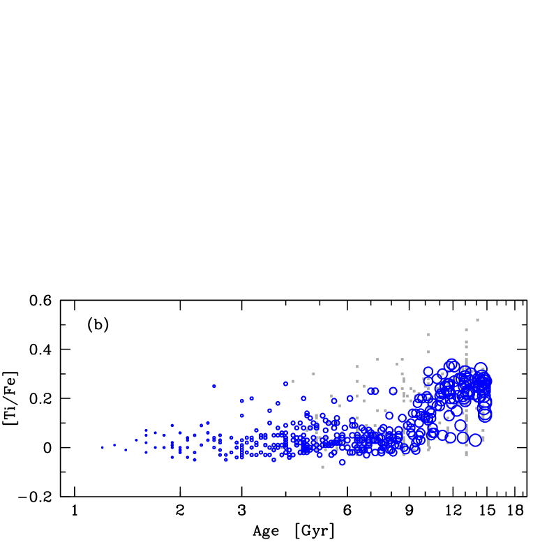
To better understand the formation and evolution of the Milky Way, it is very desirable to have stellar ages as well as elemental abundances. Given the overall structure of the elemental abundance patterns and ages observed in the Milky Way (e.g., Edvardsson et al. 1993), it has been suggested that the amount of $\alpha$-enhancement in a star can be used as a proxy for the age of a star (Liu & van de Ven 2012; Haywood et al. 2013). However, age is a very difficult property to derive for most stars (e.g., Soderblom 2010). As our sample contains a fair portion of turn-off and sub-giant stars we are in a position to investigate whether old ages are a common feature for all stars with enhanced [$\alpha$/Fe] in the Solar neighbourhood. Figure 21b shows that this is indeed the case for stars older than about 8 Gyr and thus that [Ti/Fe] can be used as a proxy for age for stars, in the sense that young and old stellar populations can be distinguished. Other studies are also finding that various $\alpha$-elements correlate with ages in this sense. For example Ramírez et al. (2013), in their Fig. 17, show the same results as our Fig. 21b, but for [O/Fe] as a function of age.

However, this result is only valid for dwarf stars in the immediate Solar neighbourhood. We do not know if the same is true elsewhere in the Galaxy or indeed recoverable for other stellar evolutionary stages. Bensby et al. (2013) provides data for 58 microlensed dwarf and turn-off stars in the Galactic bulge. These stars, tentatively, show the same trend as the stars in the Solar neighbourhood, making it plausible that the connection between $\alpha$-enhancement and age is a property shared by many stellar populations in the Galaxy.

7.1.4 A lower metallicity limit for thin disk

Thin disk stars with metallicities below $\rm[Fe/H]<-0.7$ are apparently not found in spectroscopic studies in the literature (see, e.g. Fuhrmann 2004; Reddy et al. 2003; Soubiran & Girard 2005). One of the few studies that does claim to have thin disk stars at lower metallicities, reaching $\rm[Fe/H]\approx-1$, is Mishenina et al. (2004). It is clear, however, that those few stars have chemical compositions similar to what is found in the thick disk, even though the kinematic properties place them as thin disk stars. Hence their thin disk status is ambiguous.

Out of the $>14\,000$ stars in the GCS, there are 11 010 stars that are potential thin disk stars according to their kinematics. 1378 of those stars have ages estimated to be older than 7 Gyr, and 156 stars have $\rm[M/H]<-0.7$. Our sample originally contained 27 thin disk stars with metallicity estimates in the GCS less than $\rm[Fe/H]<-0.7$. However, nine of these stars could not be analysed due to the fact that they were binaries or rotated too fast. Out of the remaining 18 stars, only one remained below $\rm[Fe/H]<-0.7$ after the spectroscopic analysis. Therefore, we believe that $\rm[Fe/H]\approx-0.7$ could be interpreted as a lower metallicity limit for the Galactic thin disk.

7.2 Metal-rich and $\alpha$-enhanced stars

Figure 22: [Ti/Fe] versus [Fe/H] for stars that have low age uncertainties (the differences between upper and lower age estimates are less than 4 Gyr). The the sizes of the circles are scaled with the ages of the stars as indicated in the figure.

Figure 23: The solid black circles mark stars that are $\alpha$-enhanced and metal-rich (HAMR stars); the empty black circles mark stars that are $\alpha$-enhanced at lower [Fe/H] (a.k.a. potential thick disk); and the small blue circles mark stars with low or moderate $\alpha$-enhancement (a.k.a. potential thin disk stars).

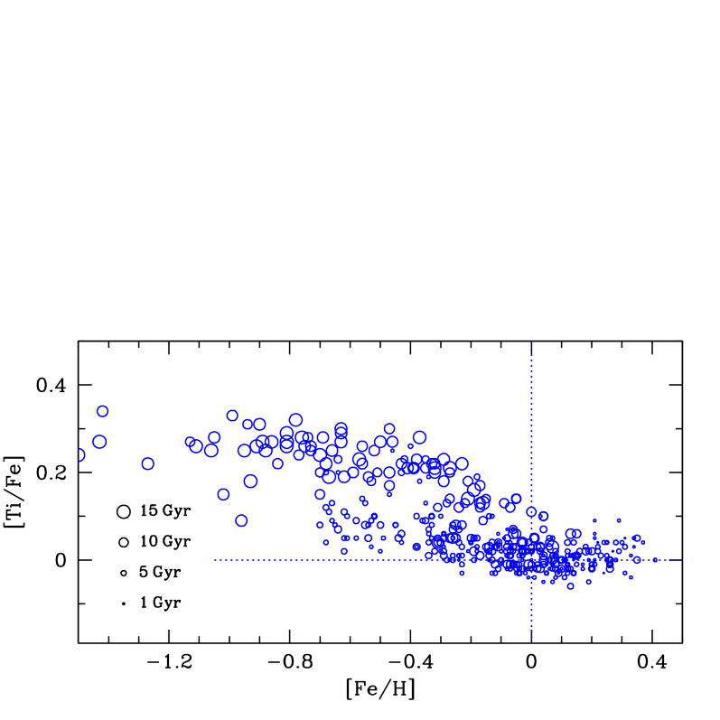
In Fig. 22 we show the [Ti/Fe] abundances trends for all stars in our sample where the upper and lower age estimates differ by at most 4 Gyr. We find a similar division of the stellar sample as seen by Fuhrmann (1998, 2000, 2004, 2008, 2011), but now in Ti. We see that the Ti-enhanced stars are the oldest stars. However, a major difference is that we have deliberately searched for metal-rich stars with hot kinematics. As a result, we have stars that could be associated with the thick disk (high $\rm[\alpha/Fe]$ ratios and high ages) that are more metal-rich than can be found in Fuhrmann’s sample (which is volume complete for $d<25$ pc and thus rarer types of stars may be missing). There are not many of them, and most of them in our sample are found outside the 25 pc sphere within which Fuhrmann’s stars are located. Hence, our sample has the potential to trace the thick disk to higher metallicities (Bensby et al. 2007b).

Figure 24: Cumulative histograms for the eccentricity, $z_{\rm max}$, and age distributions for the three different samples in Fig. 23a. HAMR stars are marked by solid black lines, potential thick disk stars by dashed black lines, and potential thin disk stars by dotted blue lines.

Figure 25: Median values of the eccentricity, $z_{\rm max}$, and age for the stars in the boxes in Fig. 23a. HAMR stars are marked by solid black circles, potential thick disk stars by open black circles, and potential thin disk stars by solid blue circles.

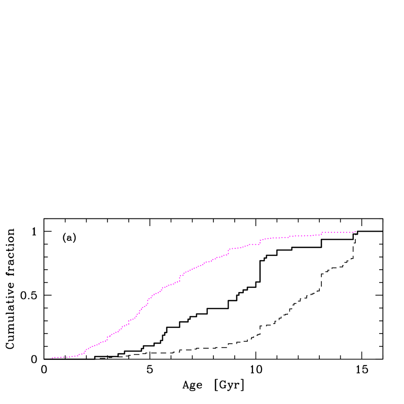
A different aspect of metal-rich and $\alpha$-enhanced stars was put forward by Adibekyan et al. (2011) who claimed a new $\alpha$-enhanced and metal-rich population (high-$\alpha$ and metal-rich stars, hereafter HAMR stars), distinct from both the thin disk and the thick disk. This HAMR population showed up as stars with [Fe/H] around solar values that have $\alpha$-enhancement greater than what is seen for the bulk of the stars at $\rm[Fe/H]\approx 0$. These stars were also separated from the thick disk by a “gap” in metallicity at $\rm[Fe/H]=-0.2$ and $\alpha$-enhancement at $\rm[\alpha/Fe]=+0.17$. The kinematical properties resembled those of the thin disk population, i.e., circular orbits confined to the Galactic plane.

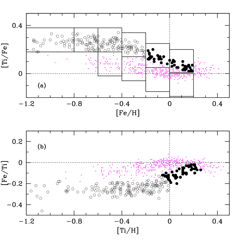
In our sample we have several stars around solar [Fe/H] that have higher $\alpha$-enhancements than the bulk of disk stars at similar metallicities (see, e.g., Figs. 15 and 22). In Fig. 23 we show the abundance trends for Ti with our HAMR stars marked by larger solid black circles, [Ti/Fe]-enhanced stars at lower [Fe/H] (typical thick disk stars) by open circles, and low-[Ti/Fe] stars (typical thin disk stars) by magenta coloured dots. The approximate separation in Fig. 23 has been done by eye. Figures 24a-c then show cumulative histograms of the age, eccentricity, and $z_{\rm max}$ distributions for these three different groups of stars. First we see that the HAMR stars have an age distribution in between those of the two disks, and that there might be “bumps” around 6-7 Gyr and 10-12 Gyr, which are the typical ages for stars of the thin and thick disks. Looking at the eccentricity and $z_{\rm max}$ distributions, it is clear that the HAMR stars are very similar to the low-$\alpha$ stars associated with the thin disk.

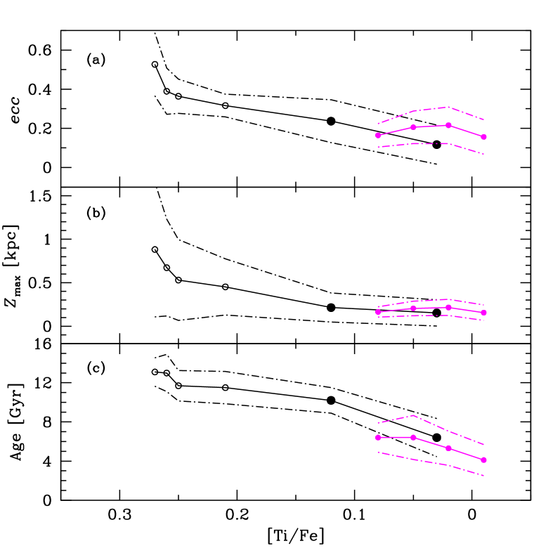
So, what are these HAMR stars, where do they come from, and should they be classified as a stellar population of their own? And if so, is there a metallicity gap between the thick disk and this newly found HAMR population? To further investigate this, we will divide the sample into “mono-abundance” populations according to the boxes in Fig. 23a. Figure 23b shows the sample but with [Ti/H] as the reference element. In Figs. 25a-c we then show how the median eccentricity, median $z_{\rm max}$, and median age varies with [Ti/Fe] for the stars in the boxes in Fig. 23a. The plots also show the 1-$\sigma$ dispersions around the median. It is evident that the eccentricity, $z_{\rm max}$, and age for the HAMR stars (black filled circles) follow smoothly upon the downward trend with [Ti/Fe] set by the “thick disk” stars (open circles). We also see that the “thin disk” stars (magenta coloured filled circles) more or less follow upon the trend set by the thick disk and HAMR stars regarding eccentricity and $z_{\rm max}$. For the ages, there could be a potential gap around 7-8 Gyr, indicating that the most metal-rich, thick disk/HAMR stars are older than the most metal-poor, thin disk stars.

In summary, we cannot claim that the HAMR stars form unique population as claimed by Adibekyan et al. (2011). More likely, it may just be the metal-rich extension of the thick disk. This implies that the thick disk potentially reaches metallicities as high as $\rm[Fe/H]\approx+0.2$, somewhat higher than what we found in Bensby et al. (2007b). The disparate results between our study and the Adibekyan et al. (2012) study could be due to that both we and them have complex selection functions. Larger samples with a controlled and well-defined selection function, such as for instance the sample from the Gaia-ESO survey (Gilmore et al. 2012), will reveal the existence or non-existence of a unique HAMR stellar population.

Figure 26: [Ti/Fe]-[Fe/H] abundance trends for stars with different $R_{\rm mean}$. Only stars for which he difference between the upper and lower age estimates is less than 4 Gyr are included. The sizes of the circles have been scaled with the ages of the stars.

7.3 Radial variation

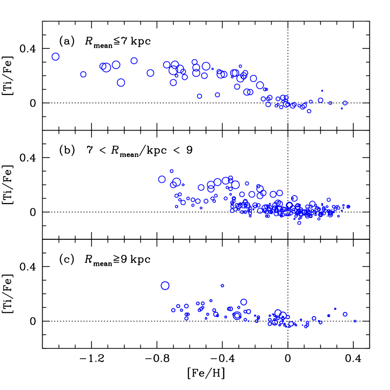
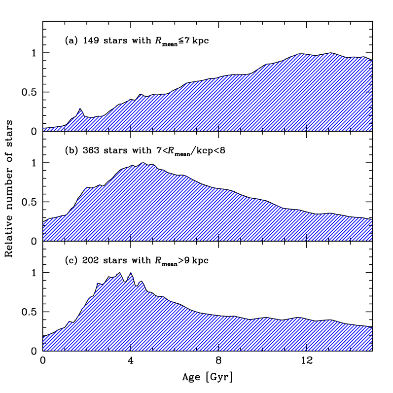
The mean of the apo- and pericentric distances of the stellar orbit, $R_{\rm mean}$, can be used as a proxy for the galactocentric radius of the birth place for a star (e.g., Grenon 1987; Edvardsson et al. 1993). However, with the recent advancement of the theory of radial migration, rearranging the orbits of stars through processes such as churning and blurring throughout the history of the Galaxy (e.g., Sellwood & Binney 2002; Schönrich & Binney 2009a, b), the usage of $R_{\rm mean}$ as a proxy for the birthplace of a star could be dubious. We will, however, start by using $R_{\rm mean}$ as a first approximation. Figure 26 shows the $\rm[Fe/Ti]-[Ti/Fe]$ trends for stars with different $R_{\rm mean}$, with the sizes of the circles scaled with the ages of the stars. We see that the sample with $R_{\rm mean}<7$ kpc mainly contains old and $\alpha$-enhanced stars with a small fraction of younger and less $\alpha$-enhanced stars. The opposite is true for the sample with $R_{\rm mean}>9$ kpc, which mainly contains young and less $\alpha$-enhanced stars and very few old and $\alpha$-enhanced stars. The sample with orbits that stay close to that of the Sun ($7<R_{\rm mean}<9$ kpc) contain stars that divide into two trends, one with old and $\alpha$-enhanced stars and one with young and less $\alpha$-enhanced stars. The age distributions in Figs. 27 further show that the sample with $R_{\rm mean}<7$ kpc contains stars of all ages with a slight over-representation of old stars; the sample of stars with orbits close to the Sun contains mainly stars with ages less than $\sim 8$ Gyr and only a few older stars; while the sample with $R_{\rm mean}>9$ kpc contains almost only younger stars. These findings indicate that the old and $\alpha$-enhanced stars mainly come from small galactocentric radii while the young and less $\alpha$-enhanced stars mainly come from large galactocentric radii.

Figure 27: Sums of individual age probability distributions for stars with different $R_{\rm mean}$. All stars are included.

Figure 28: (a) [Ni/Fe]-[Na/Fe] for the sample where the solid line marks the approximate separation between the low-$\alpha$ and high-$\alpha$ halo populations discovered by Nissen & Schuster (2010). Stars that have a total space velocity greater than $V_{\rm TOT}>180\,{\rm\,km\,s^{-1}}$ have been marked by open blue circles if located on the upper-right side of the dividing line, and by solid red circles if located on the lower-left side. (b) [Ti/Fe]-[Fe/H] for the sample with the same coding as in (a). (c) Toomre diagram with the same coding as in (a). The curved line marks $V_{\rm TOT}=180\,{\rm\,km\,s^{-1}}$. (d) Cumulative distributions of $V_{\rm TOT}$: dashed red line represents the red stars in (a)-(c), solid blue line the blue stars in (a)-(c), and dotted blue line the blue stars in (a)-(c) but only including stars with $V_{\rm TOT}>200\,{\rm\,km\,s^{-1}}$.

To address the question of whether $R_{\rm mean}$ is a valid proxy for stellar birthplace, we see that the abundance trends for the different $R_{\rm mean}$ bins in Figs. 26a–c are essentially identical to the ones found by Bensby et al. (2010, 2011b), who studied 44 red giants located in situ in the inner disk ($R=4$ to 7 kpc) and 20 red giants located in situ in the outer disk ($R=9$ to 12 kpc). Especially the lack of younger stars with low [Ti/Fe] at $\rm[Fe/H]<-0.2$ in Fig. 26a, and the lack of older $\alpha$-enhanced stars in Fig. 26c, agree very well with the inner and outer disk in situ red giant samples of Bensby et al. (2010, 2011b). These similarities could validate the use of $R_{\rm mean}$.

In Bensby et al. (2011b) the lack of $\alpha$-enhanced stars in the outer disk, even if they were located far ($>1$ kpc) from the plane, was interpreted as being due to the fact that the thick disk had a much shorter scale-length than the thin disk. Shortly thereafter, Cheng et al. (2012) used 5650 stars from the SEGUE survey and confirmed the short scale-length of the thick disk. The local data presented here appears to confirm these conclusions.

7.4 Kinematics groups and star streams

7.4.1 Low-$\alpha$ halo

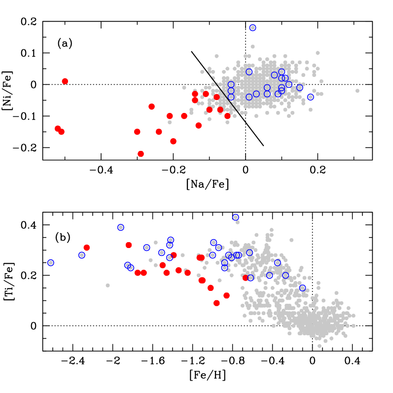
The abundance trend plots in Fig. 15 show a small number of stars with $\rm[Fe/H]\approx-1$ that have lower [Ti/Fe] than the majority of the low metallicity stars in our sample. These stars are of the same type stars as the inner halo stars found in Nissen & Schuster (1997, 2010). The selection criteria applied to their halo sample was that the stars should have $V_{\rm TOT}>180$ km s^-1, plus a metallicity criterion (derived from $uvby$ photometry). To their surprise, they found that the halo stars clearly split into two abundance trends, one with the high constant $\alpha$-enhancement, and one that shows a straight decline from $\rm[Fe/H]\approx-1.6$ to $-0.8$. Although with some overlap, the low-$\alpha$ stars identified by Nissen & Schuster (2010) generally had higher values on their total space velocities than the high-$\alpha$ ones. An even better discriminator turned out to be the [Ni/Fe]-[Na/Fe] abundance space where there was a very clear distinction, essentially without overlap, between high- and low-$\alpha$ stars.

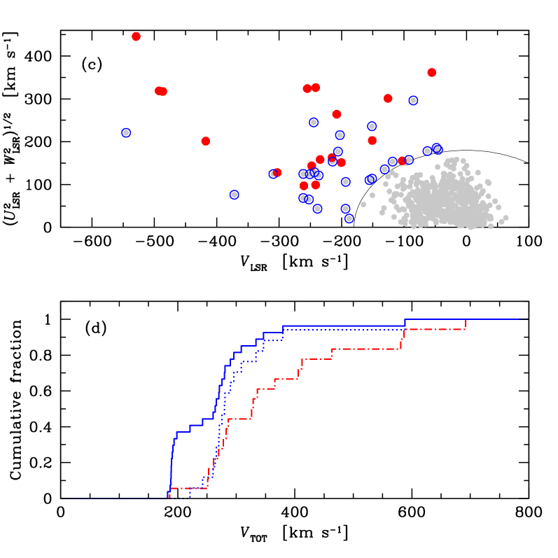
In Fig. 28a we show the [Ni/Fe]-[Na/Fe] abundance space for our stars and the dividing line found Nissen & Schuster (2010) is marked out. The stars that have ${\it V}_{\rm TOT}>180\,{\rm\,km\,s^{-1}}$ and that fall on either side of the dividing line is marked by solid red and open blue circles, respectively. Figure 28b then shows the [Ti/Fe]-[Fe/H] abundance plot with the potential high- and low-$\alpha$ stars marked. It is clear that the abundance pattern observed by Nissen & Schuster (2010) is also present in our sample, a low-$\alpha$ pattern and a high-$\alpha$ pattern the diverge with [Fe/H]. In Fig. 28c we then show the Toomre diagram with the high- and low-$\alpha$ halo stars specially marked. Although they appeared to show more different velocity distributions in the Nissen & Schuster (2010) paper, it appears as if the low-$\alpha$ halo stars in our sample on average have higher total space velocities. This is further illustrated in Fig. 28d that shows the cumulative distributions of the total space velocities for the two samples. As we have quite a few high-$\alpha$ stars (blue circles) in the Toomre diagram just outside the $V_{\rm TOT}=180\,{\rm\,km\,s^{-1}}$ line, we also show the cumulative distributions when restricting to stars with velocities greater than 200 ${\rm\,km\,s^{-1}}$.

Our results show that with our sample we can, at least tentatively, confirm the Nissen & Schuster (2010) finding that in the stellar halo, as sampled in the Solar neighbourhood, there exist two different elemental abundance trends. The different abundance trends are most likely indicative of differing origins for these stars, and should be more extensively explored with larger and complete samples, such as, e.g., the sample from the Gaia-ESO survey (Gilmore et al. 2012).

Figure 29: Stars that have kinematic probabilities of belonging to the Hercules stream ($Her/TD>2$ and $Her/D>2$) are marked by larger circles, and candidate Arcturus stream stars by larger squares. The sizes of the markers have been scaled with the ages of the stars.

Figure 30: (a) and (b) show the [Ti/Fe]-[Fe/H] abundance plots for the candidate Hercules stream and Arcturus group stars, respectively. Same markers as in Fig. 29. (c) and (d) show the cumulative age distributions for the candidate Hercules and Arcturus stars, respectively (coloured as in (a) and (b). In (c) the dotted black line represents stars with $7<R_{\rm mean}<9$ kpc and the dashed blue line stars with $R_{\rm mean}<7$ kpc (compare Fig. 26). In (d) the dashed red line represents stars with $TD/D>10$.

7.4.2 The Hercules stream

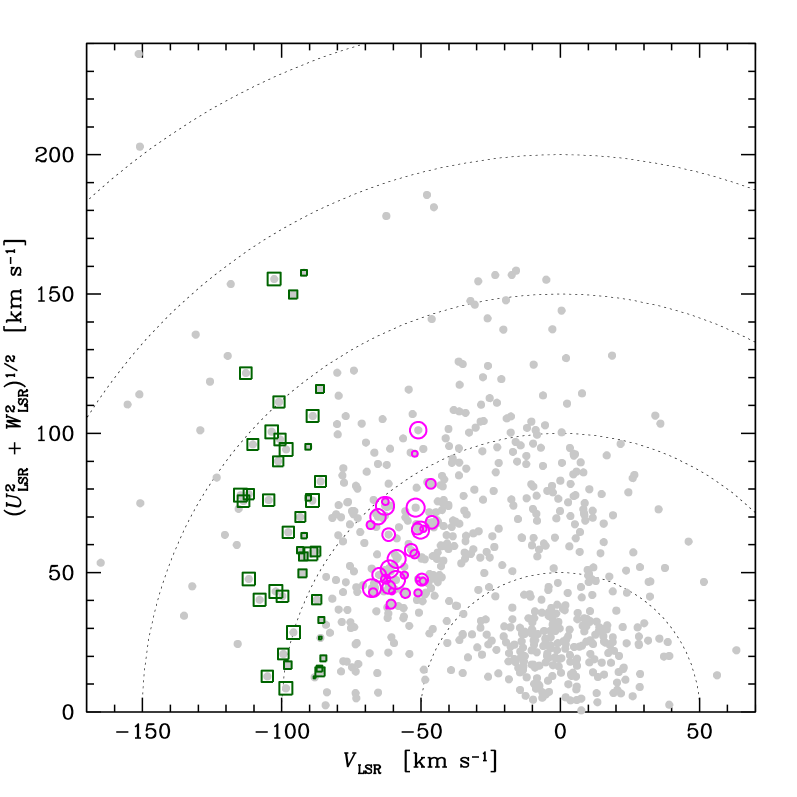
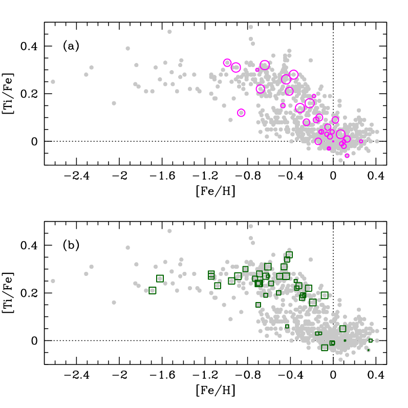
One structure of particular interest is the Hercules stream. As the Hercules stream has a net velocity drift away from the Galactic centre, it has been speculated that the Hercules stream stars have a dynamical origin in the inner parts of the Galaxy where they were kinematically heated by the central bar (e.g., Dehnen 2000; Famaey et al. 2005). In Bensby et al. (2007a) we found that stars that could kinematically be associated with the Hercules stream did not have a distinct chemical signature but showed a mixture of abundances and ages as seen in the thin and thick disks. As our analysis has been updated since the 2007 paper (see Sect. 5), and also since the comparison in Bensby et al. (2007a) was made to the smaller thin and thick disk sample of 102 stars in Bensby et al. (2005) we here reproduce the abundance plot comparison in Fig. 30a. Also, while we in Bensby et al. (2007a) chose to include all stars with kinematical probabilities $Herc/TD$ and $Herc/D$ to be greater than 1 (one), we have here required that these probability ratios should be at least 2.

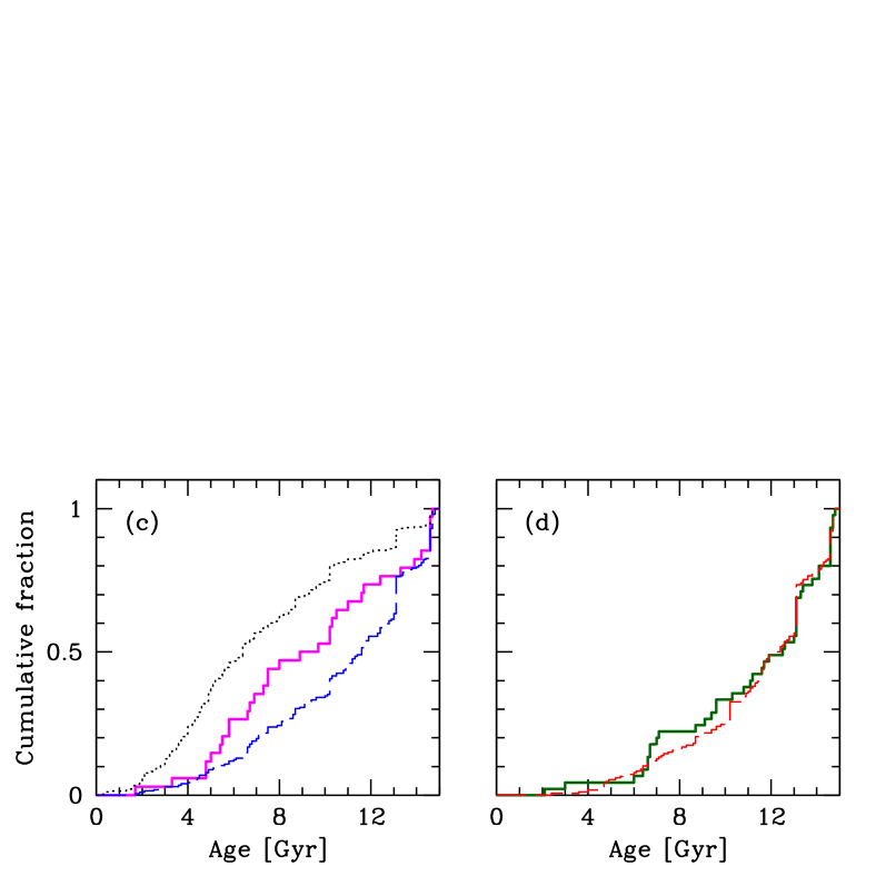
Our candidate Hercules stream stars are marked in Fig. 29a by magenta circles, and also in the corresponding abundance plot in Fig. 30a. We see that the abundance trend resembles very much the trend we see for the inner disk stars in Fig. 26a, i.e., there are $\alpha$-enhanced and old stars, as well as younger and less $\alpha$-enhanced around solar [Fe/H]. There is also a lack of low-$\alpha$ stars at lower [Fe/H], in the same way as for the inner disk sample. Figure 30c shows a comparison between the age distributions of the candidate Hercules stream stars and the “inner disk sample” that have $R_{\rm mean}<7$ kpc (dashed blue line) as well as the stars in our sample that have $7<R_{\rm mean}<9$ kpc (dotted black line). It is clear that the it does not fit either of them, but lies somewhere in between. As the Hercules stream stars have a net velocity component directed radially outwards from the Galactic centre, the resemblance is consistent with origins at slightly smaller Galactocentric radii.

7.4.3 The Arcturus moving group

Gilmore et al. (2002), and later Wyse et al. (2006), identified a group of stars lagging behind the local standard of rest (LSR) by $\sim$100 ${\rm\,km\,s^{-1}}$, that they claim to be associated with a disrupted satellite that merged with the Milky Way 10-12 Gyr ago. Navarro et al. (2004) suggest that these stars are the same group of stars that Eggen (1971) associated with the bright star Arcturus, whose Galactic orbital velocity also lags behind the LSR by $\sim$100 ${\rm\,km\,s^{-1}}$.

Both Williams et al. (2009) and Ramya et al. (2012) observed candidate members of the Arcturus moving group but could find no clear chemical signature of those stars compared to the abundance pattern seen in the Solar neighbourhood, and conclude that it most probably owes its origin to dynamical perturbations within the Galaxy.

The green squares in Fig. 29a with $-115<V_{\rm LSR}<-85\,{\rm\,km\,s^{-1}}$ mark the stars in our sample that could be associated with the Arcturus moving group. The corresponding abundance plot is shown in Fig. 30b. We find that a majority of the stars are $\alpha$-enhanced and older than 10 Gyr, and a few have younger ages and are less $\alpha$-enhanced. The general appearance is very similar to what wee see in the thick disk. The similarities to the thick disk is further demonstrated in Fig. 30d that compares the age distribution of the candidate Arcturus group stars (solid green line) with stars that are likely thick disk stars ($TD/D>10$, dashed red line). The two distributions almost identical. A two-sided $KS$-test gives $D=0.09$ and $p=0.91$, showing that the hypothesis that the two age distributions are the same cannot be rejected at the 91 % level.

The extended range in [Fe/H] and level of $\alpha$-enhancement in the candidate Arcturus group stars is very different to what is seen in dwarf galaxies (Venn et al. 2004). Instead these properties, as well as stellar ages, are very similar to what is seen in the thick disk. Hence, we conclude that there is no clear signature of an extra-galactic origin, nor disrupted cluster, for the Arcturus group, confirming the conclusions by Williams et al. 2009 and Ramya et al. 2012). The structure in velocity space associated with the Arcturus group is more likely a dynamical feature caused within the Milky Way. Actually, Gardner & Flynn (2010), and more recently Monari et al. (2013), showed that the Galactic long bar produces a kinematic feature in velocity space with the same parameters as those of the Arcturus moving group. In contrast, the short bar is believed to be responsible for the kinematic feature associated with the Hercules stream, assuming that there are, in fact, two bars.

8 Summary

We have conducted a homogeneous detailed elemental abundance study of 714 F and G dwarf stars in the Solar neighbourhood. The stars in the sample were selected on basis of their kinematics and metallicities to trace the age and abundance structures of the Galactic thin and thick disks, the stellar halo, as well as kinematic groups such as the Hercules stream and the Arcturus moving group. Hence, the selection function is very complex and the sample should not be used to infer various parameter distributions of the two disks. It is, however, well-suited to probe the properties of kinematic sub-structures in the Galactic disk and the extremes of the thin and thick disks.

The analysis is based on equivalent width measurements in high-resolution and high signal-to-noise spectra, and 1-D, LTE, plane-parallel MARCS model stellar atmospheres. Stellar parameters and abundances were determined following a purely spectroscopic approach, i.e., surface gravity from ionisation balance between Fe i and Fe ii, effective temperature from excitation balance of Fe i, and microturbulence from the balance of Fe i with reduced line strength. All Fe i abundances were corrected for NLTE effects on a line-by-line basis in every step of the analysis. We note that the excitation and ionisation balance method appears to fail for stars on the lower main sequence ($T_{\rm eff}\lesssim 5600$ K and $\log g\gtrsim 4.2$), producing an erroneously horizontal main sequence that is not seen if $\log g$ is determined from Hipparcos parallaxes. As we wanted to keep the analysis strictly spectroscopic, and distance-independent, we applied an empirical correction that was derived through comparisons to stars that have small uncertainties in their parallaxes.

In summary, our main findings and conclusions are:

1. The Solar neighbourhood appears to contain two stellar populations that have distinct, elemental abundance trends with a gap in the $\rm[\alpha/Fe]-[Fe/H]$ plane for metallicities between $\rm-0.7<[Fe/H]<-0.2$. This gap becomes more prominent if stars that are more susceptible to uncertainties ($T_{\rm eff}<5400$ K) are discarded.

2. The $\alpha$-enhanced population is old and reaches at least solar metallicities, if not higher. It also shows an age-metallicity relation, from $\sim$10 Gyr below $\rm[Fe/H]<-0.4$ to around 8 Gyr at $\rm[Fe/H]\approx 0$.

3. The $\alpha$-poor population has a lower metallicity limit around $\rm[Fe/H]\approx-0.7$. It does not show an age-metallicity relation, but a wide spread in ages (between 2-7 Gyr) over the whole metallicity range.

4. The $\alpha$-enhanced and metal-rich stars around solar [Fe/H], claimed by Adibekyan et al. (2011) to possibly be a unique population of its own, cannot be resolved as a unique population in our data set. Instead we find that it most likely is the metal-rich extension of the thick disk. The status of the HAMR stars should be further explored with a sample that has a controlled and well-defined selection function.

5. A majority of the stars that are old and $\alpha$-enhanced have Galactic orbits with $R_{\rm mean}<7$ kpc showing that their birthplaces are located in the Galactic inner disk, significantly closer to the Galactic centre than the Sun. The stars with $R_{\rm mean}>9$ kpc on the other hand, are essentially all young and less $\alpha$-enhanced. This finding is consistent with a short scale-length for the thick disk that was proposed by Bensby et al. (2011b) and later verified by Cheng et al. (2012) using the Segue G dwarf sample.

6. Our solar abundances compare within $\pm 0.05$ dex with those of nearby and young (thin disk) stars in a narrow metallicity range around $\rm[Fe/H]=0$. Hence, we cannot claim that the Sun’s abundances deviate significantly from those of other nearby disk stars.

7. Kinematical criteria to select thin and thick disk stars are significantly biased. Ages appear to be a better discriminator, but as ages with small error bars are notoriously difficult to determine, age criteria also yield samples with overlap between the two populations, although somewhat less than when using kinematical criteria.

8. The Hercules stream does not show any distinct and/or homogeneous age or abundance patterns. Hence we confirm previous findings that it most likely is a feature in velocity space produced by dynamical interactions with the Galactic (short?) bar.

9. The candidate stars of the Arcturus moving group shows an abundance pattern that very much resembles what we see in the thick disk, confirming the conclusion of Ramya et al. (2012) that it most likely is not a disrupted cluster. In addition we show that also the age distribution is very similar to what is seen in the thick disk. Although an extra-galactic origin cannot be excluded, our results most likely points to that also the Arcturus group is a dynamical feature in velocity space produced by the Galactic (long?) bar.

10. We further find that the standard 1-D, LTE, analysis where surface gravity is based on ionisation balance of abundances from Fe i and Fe ii lines, and effective temperature is based on excitation balance of abundances from Fe i lines, produces an HR-diagram with where the lower main sequence stars line up horizontally rather than showing the common steady increase in $\log g$ with decreasing $T_{\rm eff}$ on the lower main sequence. We find that this most likely is an artefact introduced by forcing ionisation balance for these stars. Where the problem lies, if it is NLTE, 3-D, or both, or something else, lies beyond the scope of the current paper. Instead we apply an empirical correction based on a comparison to stellar parameters where $\log g$ is determined from stars that have accurate Hipparcos parallaxes with uncertainties less than 5 %. From that comparison we see that stars in the turn-off, subgiant, and giant regions of the HR diagram does not seem to be affected. We also note that the ”flat main sequence syndrome” appears to be present in several other studies that utilise ionisation balance (e.g., Adibekyan et al. 2012), while other studies that utilise other methods (Hipparcos parallaxes) appears not to be hampered by the ”flat main sequence syndrome” (e.g., Reddy et al. 2003, 2006).

    That $\log g$ cannot be readily determined from ionisation balance for lower main sequence stars may be a problem for studies of distant stars where accurate distances are rarely available. Ages and spectroscopic distances will be severely affected for such stars. On the other side, studies of distant stars usually utilise turn-off or more evolved stars, for which $\log g$:s from ionisation balance appears to be on par with $\log g$:s from stars with accurate Hipparcos parallaxes.
    

The above findings show that the Milky Way indeed appears to have dual stellar populations that are chemically distinct, as well as separated in age. While the Galactic thick disk is more centrally concentrated than previously thought, the thin disk is the clearly dominant population in the outer disk, even at large distances from the Galactic plane. The epoch where we see a separation between the two disks, around 8 Gyr ago, coincides with other observational evidence for mergers between the Milky Way and another, dwarf galaxy. For instance, Gilmore et al. (2002) and Wyse et al. (2006) claim to have detected debris stars from a major merger $\sim$10 Gyr ago, and Deason et al. (2013) find that the density profile of the Milky Way halo is discontinuous, and that this break likely is associated with an early (6-9 Gyr ago) and massive accretion event.

While this paper has presented the stellar sample, the observations, analysis, and results, we are delving into greater detail on the dichotomy of the Milky Way stellar disk, and possible formation scenarios for the thick disk (Feltzing et al., 2013, in preparation).

Appendix A Kinematical selection criteria

The kinematical criteria that we have used as a starting point to select candidate thin and thick disk stars assumes that the Galactic space velocities ($U_{\rm LSR}$, $V_{\rm LSR}$, and $W_{\rm LSR}$ of the stellar populations have Gaussian distributions,

$$f=k\cdot\exp\left({-\frac{(U_{\rm LSR}-U_{\rm asym})^{2}}{2\,\sigma_{\rm U}^{2}}-\frac{(V_{\rm LSR}-V_{\rm asym})^{2}}{2\,\sigma_{\rm V}^{2}}-\frac{W^{2}_{\rm LSR}}{2\,\sigma_{\rm W}^{2}}}\right),$$ (1)

where

$$k=\frac{1}{(2\pi)^{3/2}\,\sigma_{\rm U}\sigma_{\rm V}\sigma_{\rm W}}$$ (2)

normalises the expression. $\sigma_{\rm U}$, $\sigma_{\rm V}$, and $\sigma_{\rm W}$ are the characteristic velocity dispersions, and $V_{\rm asym}$ is the asymmetric drift. The values for the velocity dispersions, rotational lags, and normalisations in the Solar neighbourhood that we used are listed in Table 4.

To get the probability (which we will call D, TD, and H, for the thin disk, thick disk, and stellar halo, respectively) that a given star belongs to a specific population the probabilities from Eq. (1) should be multiplied by the observed fractions ($X$) of each population in the Solar neighbourhood. By then dividing the thick disk probability (TD) with the thin disk (D) and halo (H) probabilities, respectively, we get two relative probabilities for the thick disk-to-thin disk (TD/D) and thick disk-to-halo (TD/H) membership, i.e.

$${\rm TD/D}=\frac{X_{\rm TD}}{X_{\rm D}}\cdot\frac{f_{\rm TD}}{f_{\rm D}},$$ (3)

and likewise for other probability ratios.

Table 4: Characteristics for stellar populations in the Solar neighbourhood.^†

	$\sigma_{\rm U}$	$\sigma_{\rm V}$	$\sigma_{\rm W}$	$U_{\rm asym}$	$V_{\rm asym}$	$X$
	———–  [km s-1]  ———–
Thin disk	35	20	16	0	$-15$	0.85
Thick disk	67	38	35	0	$-46$	0.09
Halo	160	90	90	0	$-220$	0.0015
Hercules	26	9	17	$-40$	$-50$	0.06
Arcturus	?	?	?	?	$-100$	?

Appendix B Description of error analysis method

The method is taken from Epstein et al. (2010) and is based on the fact that the four stellar parameters $m_{j}=(T_{\rm eff},\,\xi_{\rm t},\,\log g,\,\log({\rm Fe}))$ have been determined using four observables, $o_{i}$:

• $o_{1}$: The first observable is the slope from the linear regression when plotting abundances from Fe i lines versus excitation potential. For the best fit of the effective temperature ($T_{\rm eff}$) this slope should be zero;

• $o_{2}$: The second observable is the slope from the linear regression when plotting abundances from Fe i lines versus reduced line strength ($\log(W/\lambda)$). For the best fit of the micro-turbulence parameter ($\xi_{\rm t}$) this slope should be zero;

• $o_{3}$: The third observable is the abundances from Fe i and Fe ii lines. For a correctly determined surface gravity, they should be equal;

• $o_{4}$: The fourth observable is the difference between the output abundance from Fe i lines and the input metallicity of the stellar model that is used. For the best fit this difference should be zero.

Each observable can be written as a linear combination of deviations from the best fit model:

$$o_{i}=o_{i}^{0}+\sum_{j=1}^{4}b_{ij}(m_{j}-m_{j}^{0}),$$ (4)

where $b_{ij}=\partial o_{i}/\partial m_{j}=\Delta o_{i}/\Delta m_{j}$ are the partial derivatives of the observables. The values for $b_{ij}$ are determined by varying each of the stellar parameters one at a time by an amount of $\Delta m_{j}$. We choose to set $\Delta m_{1}=\pm 100$ K, $\Delta m_{2}=\pm 0.1\,{\rm\,km\,s^{-1}}$, $\Delta m_{3}=\pm 0.1$ dex, and $\Delta m_{4}=\pm 0.1$ dex. Applying these changes in the stellar parameters, we then calculate four sets of new abundances for all lines. Compared to the best fit model, we will now see changes in the observables $\Delta o_{i}=o_{i}-o_{i}^{0}$ (where $o_{i}^{0}$ is the value of the observable from the best fit model). Equation 4 gives a system of equations to be solved. Inverting the $4\times 4$ matrix of $b_{ij}$ gives a new $4\times 4$ matrix of elements $c_{ik}$. As each observable $o_{i}$ is associated with an error ($\sigma_{k}$), the uncertainties in the stellar parameters ($m_{i}$) can be then solved as:

$$\sigma(m_{i})=\sqrt{\sum_{k=1}^{4}c_{ik}^{2}\sigma_{k}^{2}}.$$ (5)

For $o_{1}$, which is the slope of the Fe i abundances versus excitation potential that is used for the determination of $T_{\rm eff}$, we take $\sigma_{1}$ as the uncertainty of the linear regression in that plot. For $o_{2}$, which is the slope of the abundances from Fe i lines versus reduced line strength, we take $\sigma_{2}$ as the uncertainty of the linear regression in that plot. For $o_{3}$, $\sigma_{3}$ is connected to the formal errors in the Fe i and Fe ii abundances. $\sigma_{4}$, associated with the observable for the balance between input and output abundances, is similar to $\sigma_{3}$, but since we only use Fe i lines to measure $\rm\log(Fe)$, we use the formal error that we measure for abundances from Fe i lines as $\sigma_{4}$. The final estimates of the uncertainties in the stellar parameters, as calculated by Eq. (5), are given together with the best fit values of the stellar parameters in Table 7.

The measured abundance of an element ($X$) can be written as a linear combination of deviations from the best fit model

$$X=X_{0}+\sum_{j=1}^{4}\kappa_{j}(m_{j}-m_{j}^{0})=X_{0}+\sum_{j=1}^{4}\alpha_{j}(o_{j}-o_{j}^{0}),$$ (6)

where the partial derivatives $\kappa_{j}=\partial X/\partial m{j}=\Delta X/\Delta m_{j}$ are calculated for all elements ($X$) by changing the stellar model atmosphere parameters by the same amounts as when determining $b_{ij}$ above, and $\alpha_{j}$ is given by

$$\alpha_{j}=\sum_{k=1}^{4}\kappa_{k}\cdot c_{kj}.$$ (7)

The error in the measured average abundance for an element then becomes

$$\sigma_{X}=\sqrt{\sigma_{X_{0}}^{2}+\sum_{k=1}^{4}\alpha_{k}^{2}\cdot\sigma_{k}^{2}}$$ (8)

where $\sigma_{k}$ are the uncertainties in the observables as given above, and $\sigma_{X_{0}}$ is the formal error of the measured abundance. The uncertainty in a measured abundance ratio [$X/Y$] is then

$$\sigma_{XY}=\sqrt{\sigma_{X}^{2}+\sigma_{Y}^{2}-2\sum_{k=1}^{4}\alpha_{k,\,X}\cdot\alpha_{k,\,Y}\cdot\sigma_{k}^{2}}$$ (9)

Uncertainties in the stellar parameters and in the abundance ratios ([$X$/Fe] and [$X$/Ti]) are given in Table 7 for all 714 stars.

Appendix C Description of online tables

We are providing three online tables. The first table (Table 5) lists the stars that were rejected from further analysis. The reasons are given in the table but the main causes are that the stars are either spectroscopic binaries and/or rotated too fast to allow for proper measurements of the equivalent widths. The next table (Table 6) gives the atomic data and the equivalent widths and elemental abundances for individual lines in the Sun. The third table (Table 7) gives the results, kinematics, ages, abundance ratios, and uncertainties for the full sample of 714 stars. Details on all three tables are given below.

Table 5: The following stars were observed but rejected from analysis. The table is only available in the online version of the paper and in electronic form at the CDS via anonymous ftp to cdsarc.u-strasbg.fr (130.79.125.5) or via http://cdsweb.u-strasbg.fr/Abstract.html

HIP	Comment
⋮	⋮
6492	Spectroscopic binary
⋮	⋮

Table 6: Atomic line data. The table is only available in the online version of the paper and in electronic form at the CDS via anonymous ftp to cdsarc.u-strasbg.fr (130.79.125.5) or via http://cdsweb.u-strasbg.fr/Abstract.html

Atom	$\lambda$		$\log gf$							Ref.
	[Å]
(1)	(2)	(3)	(4)	(5)	(6)	(7)	(8)	(9)	(10)	(11)
$\vdots$	$\vdots$	$\vdots$	$\vdots$	$\vdots$	$\vdots$	$\vdots$	$\vdots$	$\vdots$	$\vdots$	$\vdots$
Fe i	5242.491	3.634	-0.97	1.40	5.754E+07	86.2	1.00	X X	a1I z1H	BFL03
$\vdots$	$\vdots$	$\vdots$	$\vdots$	$\vdots$	$\vdots$	$\vdots$	$\vdots$	$\vdots$	$\vdots$	$\vdots$

Table 7: The online table has 714 stars with the following columns. The table is only available in the online version of the paper and in electronic form at the CDS via anonymous ftp to cdsarc.u-strasbg.fr (130.79.125.5) or via http://cdsweb.u-strasbg.fr/Abstract.html

column	label	unit	comment
(1)	HIP
(2)	$T_{\rm eff}$	K
(3)	$\epsilon(T_{\rm eff})$	K
(4)	$\log g$
(5)	$\epsilon(\log g)$
(6)	$\xi_{\rm t}$	${\rm\,km\,s^{-1}}$
(7)	$\epsilon(\xi_{\rm t})$	${\rm\,km\,s^{-1}}$
(8)	$\log\varepsilon({\rm{Fe\textsc{i}}})$		absolute abundance from Fe i lines
(9)	$\log\varepsilon({\rm{Fe\textsc{ii}}})$		absolute abundance from Fe ii lines
(10)	[Fe/H]	Sun
(11)	[O/Fe]	Sun
(12)	[Na/Fe]	Sun
(13)	[Mg/Fe]	Sun
(14)	[Al/Fe]	Sun
(15)	[Si/Fe]	Sun
(16)	[Ca/Fe]	Sun
(17)	[Ti/Fe]	Sun
(18)	[Cr/Fe]	Sun
(19)	[Ni/Fe]	Sun
(20)	[Zn/Fe]	Sun
(21)	[Y/Fe]	Sun
(22)	[Ba/Fe]	Sun
(23)	$N$(Fe i)		number of lines used
(24)	$N$(Fe ii)
(25)	$N$(O i)
(26)	$N$(Na i)
(27)	$N$(Mg i)
(28)	$N$(Si i)
(29)	$N$(Ca i)
(30)	$N$(Ti i)
(31)	$N$(Ti ii)
(32)	$N$(Cr i)
(33)	$N$(Cr ii)
(34)	$N$(Ni i)
(35)	$N$(Zn i)
(36)	$N$(Y ii)
(37)	$N$(Ba ii)
(38)	$\rm\sigma{Fe\textsc{i}}$		1-$\sigma$ line-to-line dispersion
(39)	$\rm\sigma{Fe\textsc{ii}}$
(40)	$\rm\sigma{O\textsc{i}}$
(41)	$\rm\sigma{Na\textsc{i}}$
(42)	$\rm\sigma{Mg\textsc{i}}$
(43)	$\rm\sigma{Si\textsc{i}}$
(44)	$\rm\sigma{Ca\textsc{i}}$
(45)	$\rm\sigma{Ti\textsc{i}}$
(46)	$\rm\sigma{Ti\textsc{ii}}$
(47)	$\rm\sigma{Cr\textsc{i}}$
(48)	$\rm\sigma{Cr\textsc{ii}}$
(49)	$\rm\sigma{Ni\textsc{i}}$
(50)	$\rm\sigma{Zn\textsc{i}}$
(51)	$\rm\sigma{Y\textsc{ii}}$
(52)	$\rm\sigma{Ba\textsc{ii}}$
(53)	$\rm\epsilon[Fe/H]$		abundance ratio uncertainty
(54)	$\rm\epsilon[O/Fe]$
(55)	$\rm\epsilon[Na/Fe]$
(56)	$\rm\epsilon[Mg/Fe]$
(57)	$\rm\epsilon[Al/Fe]$
(58)	$\rm\epsilon[Si/Fe]$
(59)	$\rm\epsilon[Ca/Fe]$
(60)	$\rm\epsilon[Ti/Fe]$
(61)	$\rm\epsilon[Cr/Fe]$
(62)	$\rm\epsilon[Ni/Fe]$
(63)	$\rm\epsilon[Zn/Fe]$
(64)	$\rm\epsilon[Y/Fe]$
(65)	$\rm\epsilon[Ba/Fe]$
(66)	$\rm\epsilon[Ti/H]$		abundance ratio uncertainty
(67)	$\rm\epsilon[O/Ti]$
(68)	$\rm\epsilon[Na/Ti]$
(69)	$\rm\epsilon[Mg/Ti]$
(70)	$\rm\epsilon[Al/Ti]$
(71)	$\rm\epsilon[Si/Ti]$
(72)	$\rm\epsilon[Ca/Ti]$
(73)	$\rm\epsilon[Cr/Ti]$
(74)	$\rm\epsilon[Ni/Ti]$
(75)	$\rm\epsilon[Zn/Ti]$
(76)	$\rm\epsilon[Y/Ti]$
(77)	$\rm\epsilon[Ba/Ti]$

Table 3: continued

column	label	unit	comment
(78)	Age	Gyr	Best age
(79)	Agel	Gyr	lower limit on age
(80)	Ageu	Gyr	upper limit on age
(81)	mass	sun	Best mass
(82)	massl	sun	lower limit on mass
(83)	massu	sun	upper limit on mass
(84)	$d$	kpc
(85)	$l$	deg
(86)	$b$	deg
(87)	$X$	kpc
(88)	$Y$	kpc
(89)	$Z$	kpc
(90)	$R_{\rm min}$	kpc
(91)	$R_{\rm max}$	kpc
(92)	$R_{\rm mean}$	kpc
(93)	$z_{\rm max}$	kpc
(94)	$e$
(95)	$L_{\rm Z}$
(96)	$E/E_{\rm LSR}$		total energy normalised to the LSR
(97)	$U_{\rm LSR}$	${\rm\,km\,s^{-1}}$
(98)	$V_{\rm LSR}$	${\rm\,km\,s^{-1}}$
(99)	$W_{\rm LSR}$	${\rm\,km\,s^{-1}}$
(100)	$TD/D$
(101)	$TD/H$
(102)	$Her/TD$
(103)	$Her/D$
(104)	$T_{\rm eff}$ (u.i.b)	K	un-corrected ion.bal temp
(105)	$\log g$ (u.i.b)		un-corrected ion.bal grav
(106)	$T_{\rm eff}$ (hip)	K	hipparcos temp
(107)	$\log g$ (hip)		hipparcos grav