On differential passivity of physical systems

Abstract

Differential passivity is a property that allows to check with a pointwise criterion that a system is incrementally passive, a property that is relevant to study interconnected systems in the context of regulation, synchronization, and estimation. The paper investigates how restrictive is the property, focusing on a class of open gradient systems encountered in the coenergy modeling framework of physical systems, in particular the Brayton-Moser formalism for nonlinear electrical circuits.

I Introduction

Motivated by the differential Lyapunov framework presented in [5] to study incremental stability, the recent papers [16] and [6] introduced the notion of differential dissipativity to study incremental dissipativity, the analog of incremental stability for open systems. A related notion of tranverse incremental dissipativity is presented in [10] to study limit cycles. The interest for incremental notions of stability and dissipativity stems from analysis and design problems concerned with a distance between arbitrary solutions rather than a distance to a particular (equilibrium) solution : such problems include regulation and tracking, estimation and observer design, or synchronization, coordination, and entrainment.

The differential approach to study incremental properties is rooted in contraction theory, following the influential paper of [9] in control theory. In short, incremental properties of dynamical systems can be studied differentially, through the variational equations. The analysis of the variational equation (or more precisely of the prolonged system) is appealing because it leads to pointwise conditions to be verified on the prolonged vector field rather than on the solutions, in the spirit of Lyapunov theory. The approach is geometric and the differential properties are potentially simpler to verify than their incremental counterparts.

The present paper pursues the developments of [16] and [6] to investigate how restrictive it is to check differential passivity on a given system. More fundamentally, we are interested in which class of physical systems are differentially passive and what is the physical interpretation of the property, if any. The success of passivity as an analysis and design concept of system theory stems from its clear energy interpretation in physical systems: passivity expresses that the increase of internally stored energy cannot exceed the energy supplied by the environment. It is still unclear whether a similar interpretation exists for differential passivity.

We provide geometric conditions that characterize differential passivity with respect to a quadratic storage and we further investigate the general conditions for a class of gradient systems. Our motivation stems from the fact that a broad class of physical models admits a gradient representation in the coenergy framework, see e.g. [8, 15], after the work of Brayton and Moser for nonlinear electrical circuits.

The paper provides a number of simple examples that illustrate that differential passivity may hold for a sizable class of physical models and that feedback can help achieving the property, as for passivity.

The paper is organized as follows: we revisit the notion of differential passivity in Section II, providing the definitions of prolonged and variational system, differential storage, and differential supply rate. Geometric conditions for passivity are summarized in Section III. Section IV studies the differential passivity of gradient systems. Differential passivity for Brayton-Moser systems is characterized in Section V.

Notation: Given a manifold $\mathcal{X}$, and a point $x$ of $\mathcal{X}$, $T_{x}\mathcal{X}$ denotes the tangent space of $\mathcal{X}$ at $x$. $T\mathcal{X}:=\bigcup_{x\in\mathcal{X}}\{x\}\times T_{x}\mathcal{X}$ is the tangent bundle. Given two manifolds $\mathcal{X}_{1}$ and $\mathcal{X}_{2}$ and a mapping $f:\mathcal{X}_{1}\to\mathcal{X}_{2}$, $f$ is of class $C^{k}$, $k\in\mathbb{N}$, if its coordinate representation is a $C^{k}$ function. A curve $\gamma$ on a given manifold $\mathcal{X}$ is a mapping $\gamma:I\subset{\mathbb{R}}\to\mathcal{X}$. We sometime use $\dot{\gamma}(t)$ to denote $\frac{\partial\gamma(t)}{\partial t}$.

$I_{n}$ is the identity matrix of dimension $n$. Given a vector $v$, $v^{T}$ denotes the transpose vector of $v$. Given a matrix $M$ we say that $M\geq 0$ or $M\leq 0$ if $v^{T}Mv\geq 0$ or $v^{T}Mv\leq 0$, for each $v$, respectively. Given the vectors $\{v_{1},\dots,v_{n}\}$, $\mathrm{Span}(\{v_{1},\dots,v_{n}\}):=\{v\,|\,\exists\lambda_{1},\dots\lambda_{n}\in{\mathbb{R}}\mbox{ s.t. }v=\sum_{i=1}^{n}\lambda_{i}v_{i}\}$. In coordinates, we denote the differential of a function $f$ at $x$ by $\frac{\partial f(x)}{\partial x}$. The Hessian of $f$ at $x$ is denoted by $\frac{\partial^{2}f(x)}{\partial x^{2}}$.

A distance $d:\mathcal{X}\times\mathcal{X}\to{\mathbb{R}}_{\geq 0}$ on a manifold $\mathcal{X}$ is a positive function that satisfies $d(x,y)=0$ if and only if $x=y$, for each $x,y\in\mathcal{X}$ and $d(x,z)\leq d(x,y)+d(y,z)$ for each $x,y,z\in\mathcal{X}$. A set $\mathcal{S}\subset\mathcal{X}$ is bounded if $\sup_{x,y\in\mathcal{S}}d(x,y)<\infty$ for any given distance $d$ on $\mathcal{X}$. A curve $\gamma:I\to\mathcal{X}$ is bounded when its image is bounded. Given a manifold $\mathcal{X}$, a set of isolated points $\Omega\subset\mathcal{X}$ satisfies: for any distance function $d$ on $\mathcal{X}$ and any given pair $x_{1},x_{2}$ in $\Omega$, there exists an $\varepsilon>0$ such that $d(x_{1},x_{2})\geq\varepsilon$.

II Differential passivity

II-A Prolonged systems

Consider the nonlinear system $\Sigma$ with state space $\mathcal{X}$, and inputs and outputs spaces $\mathcal{U}\subset{\mathbb{R}}^{m}$ and $\mathcal{Y}\subset{\mathbb{R}}^{m}$, respectively, given by

$$\left\{\begin{array}[]{rcl}\dot{x}&=&f(x)+g(x)u\\ y&=&h(x)\end{array}\right.$$ (1)

where $x\in\mathcal{X}$, and $u\in\mathcal{U}$, and $y\in\mathcal{Y}$. $f$ and $g_{i}$, $i\in\{1\dots m\}$ are vector fields. $h:\mathcal{X}\to\mathcal{Y}$.

Contraction analysis requires sufficient differentiability ($C^{2}$) of the solutions $\psi(t,x_{0})$ to (1), from any initial condition $x_{0}\in\mathcal{X}$ (see, e.g. [9, 12]). To enforce the desired regularity, we make the following standing assumption.

Assumption 1

$f$ and $g_{i}$, $i\in\{1\dots m\}$, are $C^{2}$ vector fields ($g_{i}$ denotes the $i$-th column of $g$). $h:\mathcal{X}\to\mathcal{Y}$ is a $C^{2}$ function. The input signal $u:{\mathbb{R}}\to\mathcal{U}$ is a $C^{2}$ function.

To a system of the form (1) one can associate the variational system given by

$$\left\{\begin{array}[]{rcl}\dot{\delta x}&=&\frac{\partial f(x)}{\partial x}\delta x+\frac{\partial g(x)u}{\partial x}\delta x+g(x)\delta u\\ \delta y&=&\frac{\partial h(x)}{\partial x}\delta x\ .\end{array}\right.$$ (2)

We call prolonged system the combination of (1) and (2), following [2, 16]. A coordinate free representation of the prolonged system is provided by the notions of complete and vertical lifts, as shown in [2, 16].

Under Assumption 1, for every solution $(x,u,y)(\cdot)$ to (1), the solutions $(\delta x,\delta u,\delta y)(\cdot)$ to (2) represent infinitesimal variations on $(x,u,y)(\cdot)$, that is, the infinitesimal mismatch between $(x,u,y)(\cdot)$ and neighboring solutions. This intuitive representation is clarified in Remark 1. Pursuing this intuition, if the dynamics of (2) guarantee that $\delta x$ converges to zero then, necessarily, the solutions to (1) must converge towards each other. A Lyapunov-based analysis of the connection between contraction of $\delta x$ and incremental stability can be found in [5].

Remark 1

For each $s\in[0,1]$ let $\gamma(s)$ be an initial condition for (1) and $u(\cdot,s)$ an input signal. Assume that $\gamma(\cdot)\in C^{2}$ and $u(\cdot,\cdot)\in C^{2}$. Then, for each $s\in[0,1]$ $x(\cdot,s)$ is a solution to (1) from the initial condition $\gamma(s)$ under the action of the input $u(\cdot,s)$. Define the displacement $\delta x(t,s):=\frac{\partial}{\partial s}x(t,s)$ and $\delta u(t,s):=\frac{\partial}{\partial s}u(t,s)$. Then, by chain rule and differentiability, we have that $\frac{d}{dt}\delta x(t,s)=\frac{\partial^{2}}{\partial s\partial t}x(t,s)=\frac{\partial}{\partial s}[f(x(t,s))+g(x(t,s))u(t,s)]=\frac{\partial f(x(t,s))}{\partial x}\delta x(t,s)+\frac{\partial g(x(t,s))u(t,s)}{\partial x}\delta x(t,s)+g(x(t,s))\delta u(t,s)$. Thus, $\delta x(\cdot,s)$ is a solution to (2) from the initial condition $\frac{\partial\gamma(s)}{\partial s}$ under the action of the input $\delta u(\cdot,s)$. Moreover, the output signal $\delta y(t,s)$ is given by $\frac{\partial y(t,s)}{\partial s}=\frac{\partial h(x(t,s))}{\partial x}\delta x(t,s)$.   $\lrcorner$

II-B Differential passivity

Henceforth we provide the notion of differential storage function and differential passivity. These notions are taken from [6, Sections 3 and 4] and restrict the definitions in [16, Section 4] to the case in which the function $P$ in [16, Definition 4.1 and Proposition 4.3] is a candidate Finsler-Lyapunov function [5]. This restriction makes possible the connection between differential passivity and incremental stability.

Definition 1

Let $\Omega$ be a set of isolated point in $\mathcal{X}$. For each $x\in\mathcal{X}$, suppose that $T_{x}\mathcal{X}$ can be subdivided into a vertical distribution $\mathcal{V}_{x}\subset T_{x}\mathcal{X}$

$$\mathcal{V}_{x}:=\mathrm{Span}(\{v_{1}(x),\dots,v_{r}(x)\})\qquad 0\leq r<d\ ,$$ (3)

and a horizontal distribution $\mathcal{H}_{x}\subseteq T_{x}\mathcal{X}$ complementary to $\mathcal{V}_{x}$, i.e. $\mathcal{V}_{x}\oplus\mathcal{H}_{x}=T_{x}\mathcal{X}$,

$$\mathcal{H}_{x}:=\mathrm{Span}(\{h_{1}(x),\dots,h_{q}(x)\})\qquad 0<q\leq d-r\,$$ (4)

where $v_{i}$, $i\in\{1,\dots,r\}$, and $h_{i}$, $i\in\{1,\dots,q\}$, are $C^{1}$ vector fields.

A function $\delta S:{T\mathcal{X}}\to{\mathbb{R}}_{\geq 0}$ is a differential storage function for the dynamical system $\Sigma$ in (1) if there exist $c_{1},c_{2}\in{\mathbb{R}}_{\geq 0}$, $p\in{\mathbb{R}}_{\geq 1}$, and a function $F:T\mathcal{X}\to{\mathbb{R}}_{\geq 0}$ such that, for each $(x,\delta x)\in T\mathcal{X}$,

$$c_{1}\,F(x,\delta x)^{p}\ \leq\ \delta S(x,\delta x)\ \leq\ c_{2}\,F(x,\delta x)^{p}\ .\qquad$$ (5)

$\delta S$ and $F$ must satisfy the following conditions. Given a set of isolated points $\Omega\subset\mathcal{X}$,

• $\delta S$ and $F$ are $C^{1}$,  $\forall x\in\mathcal{X}$, $\forall\delta x\in\mathcal{H}_{x}\setminus\{0\}$;

• $\delta S(x,\delta x)=\delta S(x,\delta x_{h})$ and $F(x,\delta x)=F(x,\delta x_{h})$,  $\forall(x,\delta x)\in T\mathcal{X}$ such that $(x,\delta x)=(x,\delta x_{h})+(x,\delta x_{v})$, $\delta x_{h}\in\mathcal{H}_{x}$, and $\delta x_{v}\in\mathcal{V}_{x}$;

• $F(x,\delta x)>0$,  $\forall x\in\mathcal{X}\setminus\Omega$ $\forall\delta x\in\mathcal{H}_{x}\setminus\{0\}$;

• $F(x,\lambda\delta x)=\lambda F(x,\delta x)$,  $\forall\lambda\!>\!0$, $\forall x\!\in\!\mathcal{X}$, $\forall\delta x\!\in\!\mathcal{H}_{x}$;

• $F(x,\delta x_{1}+\delta x_{2})<F(x,\delta x_{1})+F(x,\delta x_{2})$,  
  $\forall x\in\mathcal{X}\setminus\Omega$ and $\forall\delta x_{1},\delta x_{2}\in\mathcal{H}_{x}\setminus\{0\}$ such that $\delta x_{1}\neq\lambda\delta x_{2}$ for any given $\lambda\in{\mathbb{R}}$.

$\lrcorner$

When $\mathcal{V}_{x}=\emptyset$, $F(x,\delta x)$ provides a non symmetric norm on each tangent space $T_{x}\mathcal{X}$. A suggestive notation for $F$ is given by $|\delta x|_{x}$ which combined to (5) provides an intuitive interpretation of the differential storage function $\delta S$ as a local measure of the displacement length. For $\mathcal{V}_{x}\neq\emptyset$, it may occur that $\delta S(x,\delta x_{1})=\delta S(x,\delta x_{2})$ for $0\neq\delta x_{1}-\delta x_{2}\in\mathcal{V}_{x}$. In such a case, $\delta S$ measures the length of each $\delta x$ by looking only at its horizontal component. An example of a differential storage with $\mathcal{V}_{x}\neq 0$ is provided by $\delta S(x,\delta x)=\delta y^{T}\delta y$.

It is worth to mention that a differential storage function $\delta S$ is also a horizontal Finsler-Lyapunov function [5, Section VIII]. Therefore, $\delta S$ endows $\mathcal{X}$ with the structure of a pseudo-metric space, connecting differential passivity and incremental stability [14, 1]. An extended discussion and examples are provided in [5, Sections IV and VIII].

The notion of differential passivity introduced below is just passivity lifted to the tangent bundle.

Definition 2

The dynamical system $\Sigma$ in (1) is differentially passive if there exists a differential storage function $\delta S$ such that

$$\delta S(x(t),\delta x(t))-\delta S(x(0),\delta x(0))\leq\int_{0}^{t}\delta y(\tau)^{T}\delta u(\tau)\ d\tau$$ (6)

for all $t\geq 0$ and all solutions $(x,u,y,\delta x,\delta u,\delta y)(\cdot)$ to the prolonged system (1),(2).   $\lrcorner$

The equivalent formulation $\frac{d}{dt}\delta S(x(t),\delta x(t))\leq\delta y(t)^{T}\delta u(t)$ coincides with [16, Definition 4.1]. In comparison to passivity, differential passivity builds a relation between the energy - or cost - $\delta S$ associated to an infinitesimal variation of the solution $x(t)$, and the energy associated to an infinitesimal variation on the input/output signals. In comparison to incremental passivity [4, 13], $\delta y^{T}\delta u$ does not impose any prescribed form $\Delta y^{T}\Delta u=(y_{1}-y_{2})^{T}(u_{1}-u_{2})$ to the input/output mismatch. Instead, following Remark 1, given a parameterization $u(s),y(s)$ such that $(u(0),y(0))=(u_{1},y_{1})(\cdot)$ and $(u(1),y(1))=(u_{2},y_{2})(\cdot)$ we have that that $(y_{1}-y_{2})^{T}(u_{1}-u_{2})$ is replaced by $\int_{0}^{1}\frac{\partial y(s)}{\partial s}^{T}\frac{\partial u(s)}{\partial s}ds$. Note that $\int_{0}^{1}\frac{\partial y(s)}{\partial s}^{T}\frac{\partial u(s)}{\partial s}\ ds=\Delta y^{T}\Delta u$ only if $y(s)=sy_{1}+y_{2}(1-s)$ and $u(s)=su_{1}+u_{2}(1-s)$. This is particularly relevant at integration along solutions, since an initial parameterization satisfying the identity above at time $t=0$ does not preserve the identity for $t>0$, in general (on nonlinear models).

We conclude the section by illustrating two basic results of differential passivity. The reader is referred to [6, 16] for further results.

Theorem 1

Let $\Sigma$ in (1) be differentially passive with a differential storage $\delta S$ whose vertical distribution $\mathcal{V}_{x}=0$ for each $x\in\mathcal{X}$. Then, (1) is incrementally stable.   $\lrcorner$

Proof:

For $\delta u=0$, differential passivity guarantees that $\dot{\delta S}\leq 0$. For $\mathcal{V}_{x}=0$, $\delta S$ is a Finsler-Lyapunov function, thus incremental stability follows from [5, Theorem 1]. ∎

Theorem 2

Let $\Sigma_{1}$ and $\Sigma_{2}$ be differentially passive dynamical systems (1). Let $(u_{i},y_{i})$ be the input and the output of $\Sigma_{i}$, for $i=1,2$. Then, the dynamical system $\Sigma$ arising from the feedback interconnection

$$u_{1}=-y_{2}+v_{1}\ ,\;u_{2}=y_{1}+v_{2},$$ (7)

is differentially passive from $v=(v_{1},v_{2})\in\mathcal{U}_{1}\times\mathcal{U}_{2}$ to $y=(y_{1},y_{2})\in\mathcal{Y}_{1}\times\mathcal{Y}_{2}$.   $\lrcorner$

Proof:

Take $\delta S\!=\!\delta S_{1}\!+\!\delta S_{2}$. $\dot{\delta S}\!\leq\!\delta y_{1}\delta v_{1}\!+\!\delta y_{2}\delta v_{2}$. ∎

III The geometry of differential passivity

For quadratic differential storage functions $\delta S=\frac{1}{2}\delta x^{T}M(x)\delta x$ (Riemannian metrics), $M(x)>0$, the differential passivity of systems of the form (1) is characterized geometrically by the following conditions. For each $x\in\mathcal{X}$ and $u\in\mathcal{U}$,

$$\!\!M(x)\frac{\partial f(x)}{\partial x}+\frac{\partial f(x)}{\partial x}^{T}\!\!M(x)+\sum_{i}\frac{\partial M(x)}{\partial x_{i}}[f(x))]_{i}\leq 0$$ (8)

$$M(x)\frac{\partial g(x)u}{\partial x}+\frac{\partial g(x)u}{\partial x}^{T}\!\!M(x)+\sum_{i}\frac{\partial M(x)}{\partial x_{i}}[g(x)u]_{i}=0$$ (9)

$$\frac{\partial h(x)}{\partial x}^{T}=M(x)g(x)\ .$$ (10)

In fact, along the solutions to the prolonged system, the time derivative of $\delta S$ is given by $\dot{\delta S}=\frac{1}{2}\delta x^{T}(m_{f}(x)+m_{g}(x,u))\delta x+\delta x^{T}M(x)g(x)\delta x$, where $m_{f}(x)$ and $m_{g}(x,u)$ are given by the left-hand sides of (8) and (9), respectively.

(8) guarantees that the system is contracting for $u=0$, thus incrementally stable with respect to the geodesic distance induced by the metric $M$. The reader will notice that (8) is just the usual condition for passivity $\frac{\partial S(x)}{\partial x}f(x)\leq 0$ lifted to the tangent bundle. In a similar way, (10) guarantees that $\delta y=M(x)g(x)\delta x$, thus enforcing a differential version of the passivity condition $\frac{\partial S(x)}{\partial x}g(x)=h(x)^{T}$.

A notable difference with respect to passivity is provided by condition (9), which requires the columns of $g(x)$ to be killing vector fields for the metric $M(x)$. This guarantees that $u$ does not appear in the right-hand side of $\dot{\delta S}$, as required by (6). In this sense, the input matrix $g(x)$ restricts the class of metrics that one can use to establish differential passivity.

For the case $g(x)=B$, for example, (9) restricts the differential storage within the class of metrics $M(x)$ such that $\sum_{i}\frac{\partial M(x)}{\partial x_{i}}[Bu]_{i}=0$, which is satisfied by constant metrics $M(x)=P=P^{T}\geq 0$. In comparison to passivity, $M(x)=P$ is not an issue for linear systems

$$\left\{\begin{array}[]{rcl}\dot{x}&=&Ax+Bu\\ y&=&Cx\\ \end{array}\right.$$ (11)

($A\in{\mathbb{R}}^{n\times n}$, $B\in{\mathbb{R}}^{n\times\nu}$, and $C\in{\mathbb{R}}^{\nu\times n}$). In fact, for passive linear systems one can always find $P=P^{T}\geq 0$ such that

$$\begin{array}[]{rclcrcl}A^{T}P+PA&\leq&0&&C^{T}&=&PB\ ,\end{array}$$ (12)

which also establishes the equivalence between passivity and differential passivity for linear systems. But $M(x)=P$ determines a limitation for the satisfaction of (8) on systems of the form

$$\dot{x}=f(x)+Bu$$ (13)

since it reduces (8) to $\frac{\partial f(x)}{\partial x}^{T}P+P\frac{\partial f(x)}{\partial x}\leq 0$. This last inequality coincides with the early convergence condition of Demidovich [3]. See also [11, Theorem 2.29]. It also resembles a classical Lyapunov inequality based on quadratic Lyapunov functions and linearized vector fields. In fact, in the neighborhood of stable equilibria $x_{e}$ passivity and differential passivity are related, since locally around $x_{e}$ passive systems satisfies $\frac{\partial f(x)}{\partial x}^{T}P+P\frac{\partial f(x)}{\partial x}\leq 0$ locally around $x_{e}$.

The relevance of the condition enforced by (9) is readily illustrated by the following example.

Example 1

Consider the simple dynamics on $\mathbb{S}$ given by

$$\dot{x}=-\sin(x)+g(x)u\qquad g(x)=1\ .$$ (14)

For $g(x)=1$, (9) allows for differential storages of the form $\delta S=\frac{1}{2}\delta x^{2}$, for which $\dot{\delta S}=-\cos(x)\delta x^{2}+\delta x\delta u$. Thus, (14) is differentially passive along solution curves whose range belongs to $[-\frac{\pi}{2},\frac{\pi}{2}]$. In fact, (8) holds only for $x\in[-\frac{\pi}{2},\frac{\pi}{2}]$.

Using a non constant metric, (8) can be satisfied in the whole set $(-\pi,\pi)$. Indeed, taking

$$\delta S=M(x)\delta x^{2}\qquad M(x)=\frac{1}{1+\cos(x)}$$ (15)

(8) reads

$$-\frac{2\cos(x)}{1+\cos(x)}-\frac{\sin(x)^{2}}{(1+\cos(x))^{2}}=-1\ .$$ (16)

However, (9) does not hold, unless the input matrix $g(x)=1$ in (14) is replaced by $g(x)=\gamma\cos(\frac{x}{2})$, where $\gamma\in{\mathbb{R}}$. In such a case, following (10), (14) is differential passive with respect to the output $y=\gamma\int_{0}^{x}\frac{\cos(\frac{z}{2})}{1+\cos(z)}dz$.   $\lrcorner$

The discussion above makes clear that differential passivity for nonlinear systems of the form (1) can be established only for suitable pairs $f(x)$ and $g(x)$. The latter, through (9), defines the class of feasible metrics. The former, through (8), is required to be a contractive vector field with respect to a feasible metric (see [5, 9]). Finally, in analogy with passivity, the (differential) passivating output depends on the differential storage and on the input matrix, as established by (10).

IV Open gradient systems

IV-A General formulation and prolonged system

Given a smooth manifold $\mathcal{X}$, a Riemannian metric $Q$ on $\mathcal{X}$, and a potential function $V:\mathcal{X}\to{\mathbb{R}}$, the local coordinates representation of a gradient system is given by

$$Q(x)\dot{x}=-\frac{\partial V(x)}{\partial x}+Bu\ .$$ (17)

Following the discussion of the previous section, the study of differential passivity for gradient systems amounts to verify that $f(x):=Q(x)^{-1}\frac{\partial V(x)}{\partial x}$ and $g(x):=Q(x)^{-1}B$ satisfy (8), (9) for some differential storage $\delta S=\frac{1}{2}\delta x^{T}M(x)\delta x$.

The prolonged system is given by (17) and by the variational system

$$Q(x)\dot{\delta x}=-\left[\frac{\partial^{2}V(x)}{\partial x^{2}}\delta x\!+\!B\delta u\right]+\Gamma\!\left(x,u,\frac{\partial V(x)}{\partial x}\right)\!\delta x$$ (18)

where the matrix $\Gamma$ satisfies

$$\Gamma\!\left(x,u,\frac{\partial V(x)}{\partial x}\right)\!\delta x:=-\left[\sum_{i}\frac{\partial Q(x)}{\partial x_{i}}\delta x_{i}\right]\dot{x}\ .\\$$

$\Gamma$ is homogeneous of degree one in $\frac{\partial V(x)}{\partial x}$ and $u$, thus converges to zero as $x$ approaches an extremal point of $V$ and $u$ converges to $0$. Note that $\Gamma=0$ when $Q(x)$ is constant.

IV-B Differential passivity via natural metric and convexity

For $M(x)=Q(x)=P>0$ (constant), the differential storage $\delta S=\frac{1}{2}\delta x^{T}P\delta x$ guarantees that both (8) and (9) hold, provided that $\frac{\partial^{2}V}{\partial x^{2}}\geq 0$ for all $x\in\mathcal{X}$. In fact, along the solutions of the prolonged system, we have

$$\dot{\delta S}=-\underbrace{\delta x^{T}\frac{\partial^{2}V(x)}{\partial x^{2}}\delta x}_{\geq 0}+\delta x^{T}B\delta u\ .$$ (19)

Thus, the gradient system is differentialy passive with respect to the output $y=B^{T}x$.

The case of $Q(x)$ non constant is more involved. For $M(x)=Q(x)$ conditions (8) and (9) may not hold, in general. In fact, along the solutions of the prolonged system, the differential storage $\delta S=\frac{1}{2}\delta x^{T}Q(x)\delta x$ has derivative

$$\dot{\delta S} =-\,\delta x^{T}\frac{\partial^{2}V(x)}{\partial x^{2}}\delta x+\delta x^{T}B\delta u$$

$$+\frac{1}{2}\delta x^{T}\Gamma\left(\!x,\!u,\!\frac{\partial V(x)}{\partial x}\!\right)^{T}\!\!\!\!\delta x+\frac{1}{2}\delta x^{T}\Gamma\left(\!x,\!u,\!\frac{\partial V(x)}{\partial x}\!\right)\delta x$$

$$+\frac{1}{2}\delta x^{T}\Omega\left(\!x,\!u,\!\frac{\partial V(x)}{\partial x}\!\right)\delta x$$ (20)

where

$$\Omega\left(x,u,\frac{\partial V(x)}{\partial x}\right):=\sum_{i}\frac{\partial Q(x)}{\partial x_{i}}\dot{x}_{i}\ ;$$ (21)

and (8) and (9) are equivalent to the following inequality

$$\delta x^{T}\left(-\frac{\partial^{2}V(x)}{\partial x^{2}}+\Gamma^{T}+\Gamma+\Omega\right)\delta x\leq 0\ .$$ (22)

When (22) holds for each $(x,\delta x)\in T\mathcal{X}$ and $u\in\mathcal{U}$, then (17) is differentially passive with respect to the output $y=B^{T}u$.

Example 2

[Example 1 revised] Taking $V(x)=1-\cos(x)$ and $g(x)=1$ the dynamics in (14) reads

$$\dot{x}=-\frac{\partial V(x))}{\partial x}+u\ .$$ (23)

Note that $V(x)$ is convex in the region $[-\frac{\pi}{2},\frac{\pi}{2}]$ since $\frac{\partial^{2}V(x)}{\partial x}=\cos(x)\geq 0$ for $x\in[-\frac{\pi}{2},\frac{\pi}{2}]$. In fact, (23) is differentially passive with $\delta S=\delta x^{2}$ and $y=x$.

For $g(x)=\cos(\frac{x}{2})$, define $Q(x)=\frac{1}{\cos(\frac{x}{2})}$ and $V(x)=-4\cos(\frac{x}{2})$. Then, (14) is well defined in $(-\pi,\pi)$ and reads

$$Q(x)\dot{x}=-\frac{\sin(x)}{\cos\left(\frac{x}{2}\right)}+u=-2\sin\left(\frac{x}{2}\right)+u=-\frac{\partial V(x)}{\partial x}+u\ .$$ (24)

$V(x)$ is convex in $(-\pi,\pi)$, however differential dissipativity cannot be achieved because the term $\Gamma^{T}+\Gamma+\Omega$ in (22) shows a dependence on $u$.   $\lrcorner$

Remark 2

When (22) does not hold, we can still achieve local differential passivity under the assumption of strict convexity of $V$, for small signals $u$. Given a (sufficiently small) neighborhood $\mathcal{C}(x_{e})$, $\frac{\partial^{2}V(x)}{\partial x^{2}}>aI$ for $x\in\mathcal{C}(x_{e})$, while the last three terms in (22) are bounded by a function of the form $b(x_{e})|u||\frac{\partial V(x)}{\partial x}|$, by homogeneity. Thus, $\dot{\delta S}\leq\left(-a+b(x_{e})|u|\left|\frac{\partial V(x)}{\partial x}\right|\right)|\delta x|^{2}+\delta x^{T}B\delta u\leq\delta x^{T}B\delta u$ for $x\in C(x_{e})$ and for $|u|$ and $C(x_{e})$ sufficiently small.   $\lrcorner$

IV-C Differential passivity beyond the natural metric

We consider the case of differential storage functions $\delta S=\frac{1}{2}\delta x^{T}M(x)\delta x$ where $M(x)=Q(x)PQ(x)$ for some given matrix $P=P^{T}\geq 0$. A first consequence of the definition of $M(x)$ is that $Q$ can be relaxed to a pseudo-Riemannian metrics, that is, $Q(x)$ is not necessarily positive but still invertible. In contrast to this generalization effort, we restrict $Q$ to the class of pseudo-metrics defined by $Q(x)=\frac{\partial^{2}q(x)}{\partial x^{2}}$, where $q$ is a function differentiable sufficiently many times.

Under these assumptions, for

$$y=C\frac{\partial q(x)}{\partial x}$$ (25)

(8), (9), and (10) are equivalent to the following conditions.

Theorem 3

Consider $q:\mathcal{X}\to{\mathbb{R}}$ and $Q(x)=\frac{\partial^{2}q}{\partial x^{2}}(x)$. Then (18) is differentially passive with respect to the output $y=C\frac{\partial q(x)}{\partial x}$ if there exists a matrix $P=P^{T}\geq 0$ such that for all $x\in\mathcal{X}$

$$\frac{\partial^{2}V(x)}{\partial x^{2}}PQ(x)+Q(x)P\frac{\partial^{2}V(x)}{\partial x^{2}} \geq 0$$ (26a)

$$C^{T} = PB\,.$$ (26b)

$\delta S=\frac{1}{2}\delta x^{T}Q(x)PQ(x)\delta x$ is the differential storage   $\lrcorner$

(26a) is a generalized convexity property on $V$. We get classical convexity when $Q(x)=P=I$. For $P$ positive definite, the particular selection of the output $y=C\frac{\partial q(x)}{\partial x}$ guarantees that (17) has relative degree one. In fact, $\dot{y}=C\frac{\partial^{2}q(x)}{\partial x^{2}}\dot{x}=C(\frac{\partial V(x)}{\partial x}(x)+Bu)$, where $CB=B^{T}PB$. Finally, note that for $q(x)=V(x)$, the inequality in (26) is always satisfied. This is not surprising since, by defining $e=\frac{\partial V(x)}{\partial x}$, (17) reads $\dot{e}=-e+Bu$, $y=Ce$.

Proof of Theorem 3: Define $f(x):=\left[\frac{\partial^{2}q(x)}{\partial x^{2}}\right]^{-1}\frac{\partial V(x)}{\partial x}$, $g(x):=\left[\frac{\partial^{2}q(x)}{\partial x^{2}}\right]^{-1}Bu$, and $h(x):=C^{T}\frac{\partial q(x)}{\partial x}$, and consider the prolonged system (1),(2). By exploiting the differentiability of $q$, and using the chain rule,

$$\begin{array}[]{rcl}\dot{\delta S}\!\!&\!\!=\!\!&\!\!\!\delta x^{T}Q(x)P\!\left[\dfrac{\partial[Q(x)f(x)]}{\partial x}\delta x+\dfrac{\partial[Q(x)g(x)u]}{\partial x}\right]\delta x\vspace{1mm}\\ &&+\ \delta x^{T}Q(x)PQ(x)g(x)\delta u\vspace{2mm}\\ &=&\underbrace{\delta x^{T}Q(x)P\dfrac{\partial V(x)}{\partial x}\delta x}_{\leq 0}+\ \delta x^{T}Q(x)P\underbrace{\dfrac{\partial[Bu]}{\partial x}}_{=0}\delta x\\ &&\ +\ \delta x^{T}Q(x)\underbrace{PB}_{C^{T}}\delta u\vspace{2mm}\\ &\leq&\delta x^{T}Q(x)C^{T}\delta u\ =\ \delta y^{T}\delta u\ .\end{array}$$ (27)

(8), (9), (10) read $\delta x^{T}Q(x)P\frac{\partial V(x)}{\partial x}\delta x\leq 0$, $\delta x^{T}Q(x)P\frac{\partial[Bu]}{\partial x}\delta x=0$, and $\delta x^{T}Q(x)PB=\delta xQ(x)C^{T}$, respectively.   $\blacksquare$

Remark 3

Theorem 3 extends to systems of the form

$$Q(x)\dot{x}=A(x)+Bu$$ (28)

where $A(x)$ is a vector field not derived from a potential. In this case, $\frac{\partial^{2}V(x)}{\partial x^{2}}$ in (26a) is replaced by $\frac{\partial A(x)}{\partial x}$.   $\lrcorner$

Example 3

[Example 2 revised] Consider the system formulation given in (24) for the case $g(x)=\cos\left(\frac{x}{2}\right)$. Take the differential storage $\delta S=\frac{1}{2}\delta x^{T}Q(x)PQ(x)\delta x$ for $P=1$. Then, from Theorem 3, the inequality (26a) reads

$$2\frac{\cos\left(\frac{x}{2}\right)}{\cos\left(\frac{x}{2}\right)}=2\geq 0\ ,$$ (29)

and (24) is differentially passive in $(-\pi,\pi)$ with respect to the output $y=\int_{0}^{x}Q(z)dz$. Because (29) is strictly positive, the system is incrementally asymptotically stable. The solutions converge to the unique steady-state solution compatible with the input signal $u$ [5] (see Fig 1).

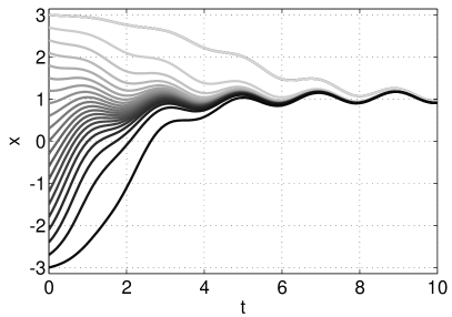
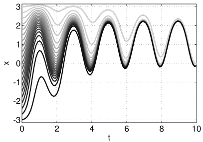
Figure 1: Entrainment of (24) with $g(x)=\cos\left(\frac{x}{2}\right)$ for the (small) input $u=1+0.5\sin(\pi t)$, left, and the (large) input $u=1+5\sin(\pi t)$, right.

$\lrcorner$

V Brayton-Moser systems

V-A Passivity conditions

The approach developed in the previous section allows for the analysis of the passivity of Brayton-Moser systems [7, 8, 15]. Brayton-Moser modeling of physical systems characterizes a class of gradient systems of the form

$$Q(z)\dot{z}=\frac{\partial V(z,u)}{\partial z}\ ,$$ (30)

where the state-s[ace is given by flow and efforts $z=(f,e)$, $V$ is a the potential, and $Q(z)$ satisfies

$$Q(z)=\left[\begin{array}[]{cc}-\frac{\partial^{2}H^{*}(f,e)}{\partial f^{2}}&0\\ 0&\frac{\partial^{2}H^{*}(f,e)}{\partial e^{2}}\end{array}\right]\ .$$ (31)

$H^{*}$ is the Legendre transform of the Hamiltonian $H$. In relation to the theory developed in the previous section, we assume that $H^{*}$ has the following structure

$$H^{*}(f,e)=H^{*}_{f}(f)+H^{*}_{e}(e)$$ (32)

which guarantees that $Q(z)=\frac{\partial^{2}[-H^{*}_{f}(f)+H^{*}_{e}(e)]}{\partial z^{2}}$. In a similar way, we assume that $V$ has the form

$$V(z,u)=p(z)+z^{T}Bu\ .$$ (33)

Under these assumptions, (30) reads

$$\frac{\partial^{2}H^{*}(z)}{\partial z^{2}}\dot{z}=\frac{\partial p(z)}{\partial z}+Bu\ .$$ (34)

From Theorem 3, the system (34) is differential passive with respect to the output $y=B^{T}\frac{\partial H^{*}(z)}{\partial z}$, if

$$\frac{\partial^{2}H^{*}(z)}{\partial z^{2}}\frac{\partial^{2}p(z)}{\partial z^{2}}+\frac{\partial^{2}p(z)}{\partial z^{2}}\frac{\partial^{2}H^{*}(z)}{\partial z^{2}}\leq 0\ .$$ (35)

The reader will notice that the output $y=B^{T}\frac{\partial H^{*}(z)}{\partial z}$ is not the usual passive output $y_{p}=B^{T}z$. However, $y$ and $y_{p}$ show an intriguing duality, through energy and co-energy formulation of the system [15, Section 4].

V-B Differential passivity of a nonlinear RC circuit

The behavior of the nonlinear circuit represented in Figure 2 is captured by the following equations:

$$\dot{q}=-i_{r}+i,\ \\ i_{r}=R(v),\ \ v=\frac{\partial h}{\partial q}(q),\,q=C(v)=\frac{\partial h^{*}}{\partial v}(v)\ .$$

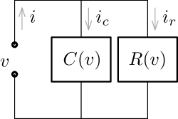
Figure 2: $V$,$I$ - external voltage and current. $v_{c}$,$i_{c}$ - capacitor voltage and current. $v_{r}$,$i_{r}$ - resistor voltage and current.

Defining $Q(v)=\frac{d^{2}h^{*}}{dv^{2}}(v)$, we get the gradient system

$$Q(v)\dot{v}=-R(v)+i\ .$$ (36)

From Theorem 3, differential passivity can be achieved if $Q(v)\frac{\partial R(v)}{\partial v}\geq 0$. In fact, defining $\delta S(v,\delta v)=\frac{1}{2}(Q(v)\delta v)^{2}$, we have that

$$\dot{S}=-Q(v)\frac{\partial R(v)}{\partial v}\delta v^{2}+Q(v)\delta v\delta i\ .$$ (37)

Therefore, if $R(v)$ is not decreasing and $\frac{\partial h^{*}(v)}{\partial v}$ is strictly increasing, we get

$$\dot{S}\ \leq\ Q(v)\delta v\delta i\ =\ \delta q\delta i\ .$$ (38)

For example, suppose that $v$ can only take positive values, and take $R(v)=v^{5}$. $R(v)$ models a nonlinear resistor $v=\tilde{R}(i)i$ whose value $\tilde{R}(i)$ decreases as $i$ increases. For the capacitor, consider the relation $C(v)=\frac{\partial h^{*}}{\partial v}(v)=\log(1+v)$, to model a saturation effect on the capacitor plates, where the charge on the plates grows at sub-linear rate with respect to the voltage. Note that $Q(v)=\frac{1}{1+v}>0$ for $v\geq 0$.

The incremental stability property of the circuit is clearly visible in the left part of Figure 3. The steady-state behavior of the circuit is independent from the initial condition, (nonlinear filter).

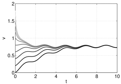
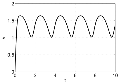
Figure 3: Contraction and nonlinear behavior of the nonlinear RC circuit. The left figure illustrates contraction for a broad range of initial conditions. The right figure illustrates the nonlinear response of the circuit to a large harmonic input signal.

V-C Differential passivation of the rigid body

Let us consider the rigid-body dynamics given by

$$\begin{array}[]{rcl}\left[\begin{smallmatrix}I_{1}&0&0\\ 0&I_{2}&0\\ 0&0&I_{3}\end{smallmatrix}\right]\dot{w}\!\!&\!\!=\!\!&\!\!\left[\begin{smallmatrix}I_{2}-I_{3}&0&0\\ 0&I_{3}-I_{1}&0\\ 0&0&I_{1}-I_{2}\end{smallmatrix}\right]\!\!\left[\begin{array}[]{c}\!\omega_{2}\omega_{3}\!\\ \!\omega_{1}\omega_{3}\!\\ \!\omega_{1}\omega_{2}\!\end{array}\right]+u\end{array}$$ (39)

where $\omega_{k}$ and $I_{k}$ are the angular velocities of the body with respect to the axis of a frame fixed to the body, and the principle moments of inertia.

Suppose that $I_{1}>I_{2}>I_{3}$ and define

$$\begin{array}[]{rcl}I&:=&\mathrm{diag}(I_{1},I_{2},I_{3})\\ \tilde{Q}&:=&\mathrm{diag}(I_{2}-I_{3},I_{3}-I_{1},I_{1}-I_{2})\\ Q&:=&I\tilde{Q}^{-1}\\ p(\omega)&:=&\omega_{1}\omega_{2}\omega_{3}\\ \end{array}$$ (40)

then we can rewrite the rigid body dynamics as follows

$$Q\dot{\omega}=\frac{\partial p(\omega)}{\partial\omega}+\tilde{Q}^{-1}u\qquad(q(\omega)=\frac{1}{2}\frac{\partial^{2}\omega^{T}Q\omega}{\partial\omega^{2}})\ .$$ (41)

Furthermore, let us consider a passivation design given by

$$u=I(-r(\omega)+Gv)\ ,\quad r(\omega):=\left[\begin{array}[]{ccc}r_{1}\omega_{1}&r_{2}\omega_{2}&r_{3}\omega_{3}\end{array}\right]^{T}.$$ (42)

(41) becomes

$$Q\dot{\omega}=\frac{\partial p(\omega)}{\partial\omega}-Qr(\omega)+QGv\ .$$ (43)

From Theorem 3, picking $P=Q^{-2}$, (26a) reads

$$Q^{-1}\frac{\partial^{2}p(\omega)}{\partial\omega^{2}}+\frac{\partial^{2}p(\omega)}{\partial\omega^{2}}Q^{-1}-2\frac{\partial r(\omega)}{\partial\omega}\leq 0$$ (44)

while condition (26a) becomes $C^{T}=Q^{-1}G$. Therefore, differential passivity from $v$ to $y=G^{T}\omega$ can be guaranteed semi-globally, since for any given compact region of velocities, there exists a selection of $r_{1},r_{2},r_{3}$ that guarantees (44) within that region.

For $I_{1}=3$, $I_{2}=2$, $I_{3}=1$ and $r_{1}=r_{2}=r_{3}=0.2$, to achieve a desired steady-state solution $[d(t),0,0]^{T}$ it is sufficient to define $G=[1,0,0]^{T}$ and $v=r_{1}d(t)+\dot{d}(t)$, as shown on the left of Figure 4 for $d(t)=3\sin(\pi t)$. Using differential passivity, we can improve the convergence rate by output feedback $v=-0.5y+(r_{1}+0.5)d(t)+\dot{d}(t)$, as shown in the simulation on the right.

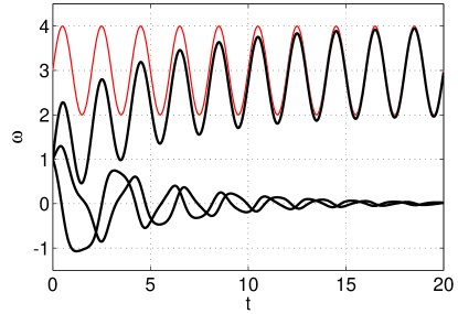
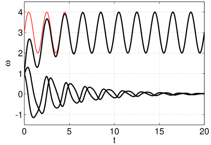
Figure 4: The passivation design on the rigid body guarantees contraction. The left figure illustrates the contraction of the three states. Output injection $y=G^{T}\omega$ improves the convergence rate, as illustrated by the right figure.

VI Conclusions

Building upon [6] and [16], we introduced the notion of differential passivity and we proposed geometric conditions for differential passivity of gradient and Brayton-Moser systems. The meaning and the feasibility of such conditions is investigated through detailed discussion and several examples. Examples suggests that differential passivity may hold for a sizeable class of physical models.

References

- [1] D. Bao, S.S. Chern, and Z. Shen. An Introduction to Riemann-Finsler Geometry. Springer-Verlag New York, Inc. (2000), 2000.
- [2] P.E. Crouch and A.J. van der Schaft. Variational and Hamiltonian control systems. Lecture notes in control and information sciences. Springer, 1987.
- [3] B.P. Demidovich. Dissipativity of a system of nonlinear differential equations in the large. Uspekhi Mat. Nauk, 16(3(99)):216, 1961.
- [4] C.A. Desoer and M. Vidyasagar. Feedback Systems: Input-Output Properties, volume 55 of Classics in Applied Mathematics. Society for Industrial and Applied Mathematics, 1975.
- [5] F. Forni and R. Sepulchre. A differential Lyapunov framework for contraction analysis. http://arxiv.org/abs/1208.2943, 2012.
- [6] F. Forni and R. Sepulchre. On differentially dissipative dynamical systems. In 9th IFAC Symposium on Nonlinear Control Systems, 2013.
- [7] D. Jeltsema and J.M.A. Scherpen. A dual relation between port-Hamiltonian systems and the Brayton-Moser equations for nonlinear switched rlc circuits. Automatica, 39(6):969 – 979, 2003.
- [8] D. Jeltsema and J.M.A. Scherpen. Multidomain modeling of nonlinear networks and systems. Control Systems, IEEE, 29(4):28 –59, 2009.
- [9] W. Lohmiller and J.E. Slotine. On contraction analysis for non-linear systems. Automatica, 34(6):683–696, June 1998.
- [10] I.R. Manchester and J.E. Slotine. Contraction criteria for existence, stability, and robustness of a limit cycle. arXiv, 2013.
- [11] A. Pavlov, N. van de van de Wouw, and H. Nijmeijer. Uniform output regulation of nonlinear systems: A convergent dynamics approach, 2005.
- [12] G. Russo, M. Di Bernardo, and E.D. Sontag. Global entrainment of transcriptional systems to periodic inputs. PLoS Computational Biology, 6(4):e1000739, 04 2010.
- [13] G.B. Stan and R. Sepulchre. Analysis of interconnected oscillators by dissipativity theory. IEEE Transactions on Automatic Control, 52(2):256 –270, 2007.
- [14] L. Tamássy. Relation between metric spaces and Finsler spaces. Differential Geometry and its Applications, 26(5):483 – 494, 2008.
- [15] A.J. van der Schaft. On the relation between port-Hamiltonian and gradient systems. In Proceedings of the 18th IFAC World Congress, pages 3321–3326, 2011.
- [16] A.J. van der Schaft. On differential passivity. In 9th IFAC Symposium on Nonlinear Control Systems, 2013.