Learning Based Uplink Interference Management in 4G LTE Cellular Systems

Abstract

LTE’s uplink (UL) efficiency critically depends on how the interference across different cells is controlled. The unique characteristics of LTE’s modulation and UL resource assignment poses considerable challenges in achieving this goal because most LTE deployments have 1:1 frequency re-use, and the uplink interference can vary considerably across successive time slots. In this work, we propose LeAP, a measurement data-driven machine learning paradigm for power control to manage uplink interference in LTE. The data driven approach has the inherent advantage that the solution adapts based on network traffic, propagation and network topology, that is increasingly heterogeneous with multiple cell-overlays. LeAP system design consists of the following components: (i) design of user equipment (UE) measurement statistics that are succinct, yet expressive enough to capture the network dynamics, and (ii) design of two learning based algorithms that use the reported measurements to set the power control parameters and optimize the network performance. LeAP is standards compliant and can be implemented in centralized SON (self organized networking) server resource (cloud). We perform extensive evaluations using radio network plans from real LTE network operational in a major metro area in United States. Our results show that, compared to existing approaches, LeAP provides $4.9\times$ gain in the $20^{th}\%-\text{tile}$ of user data rate, $3.25\times$ gain in median data rate.

I Introduction

LTE uplink (UL) consists of a single carrier frequency division multiple access (SC-FDMA) technique that orthogonalizes different users transmissions in the same cell, by explicit assignments of groups of DFT-precoded orthogonal subcarriers. This is fundamentally different from 3G, where users interfered with each other over the carrier bandwidth and advanced receivers, such as successive interference cancellers, were employed to suppress same cell interference. Same cell interference is mitigated by design in LTE, however, other cell interference has a very different structure compared to 3G. This calls for new power control techniques for setting user transmit power and managing uplink interference. In this paper, we design and evaluate LeAP, a new system that uses measurement data to set power control parameters for optimal uplink interference management in LTE.

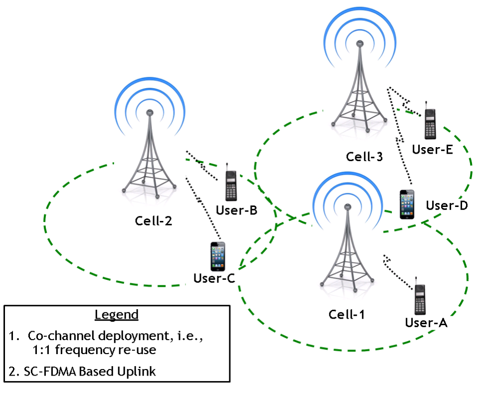
Figure 1: An illustration of three adjacent LTE cells. Depending on MAC time-frequency assignment to users in Cell-2, 3, uplink transmission of User-A in Cell-1 could receive high interference from Cell-2 and low interference from Cell-3 or vice versa.

I-A Uplink interference in 4G systems: Distinctive Properties

Uplink interference in cellular systems is managed through careful power control which has been a topic of extensive research for more than two decades (see Section II). However, uplink interference in LTE networks needs to be managed over multiple narrow bands (each corresponding to collection of a few sub-carriers) over the entire bandwidth, thus giving rise to unique research challenges.

To understand this better, we start by making two observations. Firstly, the uplink data rate of a user in LTE depends on the SINR over the resource blocks (RBs) assigned to the transmission. Secondly, LTE uses 1:1 frequency re-use and thus an RB assigned to a user in a cell can be used by another user in any of the neighboring cells too. The following example illustrates how uplink interference is impacted due to the above observations.

Example: Consider the system in Figure 1 with three cells. Suppose the MAC of Cell-1 assigns, to an associated User-A, RBs corresponding to time-frequency tuples $(ts_{1},fb_{1}),(ts_{2},fb_{2})$ over consecutive time slots $ts_{1},ts_{2}$ respectively. Since the MAC of Cell-2 and Cell-3 operate independently and use the same carrier frequency due to 1:1 re-use, the MAC assignments of time-frequency tuples $(ts_{i},fb_{j}),\ i,j=1,2$ at Cell-2 and Cell-3 could potentially be the following:

• Cell-2: $(ts_{1},fb_{1})\rightarrow\text{User-C}$ and $(ts_{2},fb_{2})\rightarrow\text{User-B}$

• Cell-3: $(ts_{1},fb_{1})\rightarrow\text{User-E}$ and $(ts_{2},fb_{2})\rightarrow\text{User-D}$

As shown in the figure, since User-C and User-D are close to the edge of Cell-1, in $ts_{1}$, User-A’s transmission receives high interference from Cell-2 and low interference from Cell-3, whereas, in $ts_{2}$, User-A’s transmission receives high interference from Cell-3 and low interference from Cell-2. In any arbitrary time-frequency resource, interfering signal to User-A’s uplink transmission at Cell-1, denoted by $\text{Int}_{A}(LTE)$, can be expressed as

$${\text{Int}}_{A}(LTE)=P_{B}\boldsymbol{1}_{B}+P_{C}\boldsymbol{1}_{C}+P_{D}\boldsymbol{1}_{D}+P_{E}\boldsymbol{1}_{E}\ ,$$

where, $P_{U},U\in\{B,C,D,E\}$ denotes the received power at Cell-1’s base station due to potential uplink transmission of User-U in the same frequency block as User-A, and, $\boldsymbol{1}_{U},U\in\{B,C,D,E\}$ is an $0\--1$ indicator variable denoting whether User-U also transmits over the same time-frequency block as User-A. Note that, since User-B and User-C share the same cell, only one of them can be active in a time-frequency resource and thus $\boldsymbol{1}_{B}+\boldsymbol{1}_{C}\leq 1$; similarly $\boldsymbol{1}_{D}+\boldsymbol{1}_{E}\leq 1$. Since MAC of each neighboring cell makes independent scheduling decision on who gets scheduled in a time-frequency block, the interference becomes highly unpredictable from transmission to transmission; managing this unstable interference pattern poses unique research challenges barely addressed in the literature. Indeed, this is unlike 3G systems , where the neighboring cell interference for a similar topology with CDMA technology (over an appropriate CDMA channel) would simply be

$$\text{Int}_{A}(CDMA)=P_{B}+P_{C}+P_{D}+P_{E}$$

thus leading to a more stable interference pattern across transmissions. In general, unlike LTE, the overall CDMA uplink interference also has an additional term for self cell interference due to uplink users in the same cell. Of course, for desirable user performance, the uplink interference still has to be managed through power control algorithms that has been the focus of much of the existing research on 3G power control and uplink interference management.

Solution requirements: LTE networks are deployed with self organized networking (SON) capabilities [1, 2] to maximize network performances. Today’s LTE networks are also heterogeneous (HTNs) that include high power macro cells overlaying low power small (pico/femto) cells. Small cells are deployed in traffic hotspots or coverage challenged areas, and thus, typically small cells outnumber macros by an order of magnitude. This leads to a much larger, and hence more difficult to tune and manage, cellular network where centralized SON servers are deployed to continuously optimize the network [1]. Thus, a good solution to uplink interference management should satisfy the following requirements: (i) it should be adaptive to network traffic, propagation geometry and topology, (ii) it should scale with the size of the network which could consist of tens of thousands of cells, and (iii) it should be architecturally compliant in the sense that it is implementable in a SON server and adherent to standards. Note that, SON implementability dictates that the solution makes use of the large amount of network measurement data. In this paper, we design a solution that satisfy these requirements and achieves high network performance.

I-B Our Contributions

In this paper, we propose LeAP, a learning based adaptive power control for uplink interference management in LTE systems. We make the following contributions:

• New framework for measurement data driven uplink interference management: We propose a measurement data driven framework for setting power control parameters for optimal uplink interference management in an LTE network. Our framework (i) models the unique interference pattern in OFDMA based LTE systems, (ii) accounts for varying traffic load and diverse propagation map in different cells, (iii) and is implementable in a centralized SON architecture. See Section IV-V.

• Design of Measurement Statistics: We derive suitable measurement statistics based on the processing of raw data from UE measurement reports. Our measurement statistics are succinct yet expressive enough to optimize the uplink performance by accounting for LTE’s unique uplink interference patterns along with network state and parameters. See Section V for details.

• Design of learning based algorithms: Using the measurements derived in Section V, we propose two learning based algorithms for optimal setting of cell-specific power control parameters in LTE networks. The two algorithms trade-off complexity and performance: one provably converges to the optimal, and the other is a fast heuristic that can be implemented using off-the-shelf solvers. See Section VI-VII.

• Extensive evaluation of LeAP benefits: We evaluate our design using a radio network plan from a real LTE network deployed in a major US metro. We demonstrate the substantial gains for the evaluated network: the edge data rate ($20^{th}\%-\text{tile}$ of data rate) improves to $4.9\times$ whereas the median gain improves to $3.25\times$ compared to existing approaches. The details are in Section VIII.

II Related Work

Cellular Power Control: Uplink power control in cellular systems has been an active research area for around three decades. The pioneering works in [38, 19] developed principles and iterative algorithms to achieve target SINR when multiple users simultaneously transmit over a shared carrier. This model is applicable to CDMA (3G) systems uplinks. Since then, several authors have developed algorithms to jointly optimize rate and transmit power in similar multi-user systems [32, 12, 23, 37]. In particular, [32, 23, 37] consider utility based framework for joint optimization of rate and transmit power. Uplink power control optimization was made tractable in CDMA setting in [10, 35] where log-convexity of feasible SINR region was shown. We refer the reader to [13] for an excellent survey of the vast body of research in power control. However, the uplink model in LTE is fundamentally different from these systems for two reasons. First, unlike CDMA, uplink interference in LTE is only from neighboring cells and the interference over an assigned frequency block could change in every transmission, leading to a far more variable interference pattern. Secondly, to control neighboring cell interference, the standards have mandated cell-specific power control parameters that in turn govern UE SINR-targets.

Fractional Power Control (FPC) in LTE: LTE power control is FPC based which has led to some recent work [6, 18, 14, 17]. However, unlike our work, none of previous publications develop a framework and associated algorithms to optimize the FPC parameters based on user path loss statistics and traffic load. Recognizing the difficulties of setting FPC parameters in LTE, [39] develops and evaluates closed loop power control algorithms for dynamically adjusting SINR targets so as to achieve a fixed or given interference target at every cell. This work has two drawbacks: first, it is unclear how the interference targets could be dynamically set based on network and traffic dynamics, and second, the scheme does not maximize any “network-wide” SON objective.

Self Organized Networking (SON) in LTE: Study of LTE SON algorithms have gained some attention recently mostly for downlink related problems. [31, 28] study the problem of downlink inter-cell interference coordination (ICIC) for LTE, [34] optimizes downlink transmit power profiles in different frequency carriers, and [27, 36, 24, 33] study various forms (downlink, uplink, mobility based etc.) of traffic-load balancing with LTE SON. To our best knowledge, ours is the first work to develop measurement data-driven SON algorithms for uplink power control in LTE. For a very extensive collection of material and presentations on the latest industry developments in LTE SON, we refer the reader to [1, 2].

III A Primer on LTE Uplink and Fractional Power Control

Terminologies used in the paper: A resource block (henceforth RB) is a block of 12 sub-carriers and 7 OFDM symbols and is the smallest allocatable resource in the frequency-time domain. eNodeB (eNB in short) refers to an LTE base station and it hosts critical protocol layers like PHY, MAC, and Radio Link Control etc. User equipment (henceforth UE) refers to mobile terminal or user end device, and we also use UL for uplink. Finally, reference signal received power (RSRP) is the average received power of all downlink reference signals across the entire bandwidth as measured by a UE. RSRP is a measure of downlink signal strength at UE.

III-A UL Transmission in LTE

LTE uplink uses SC-FDMA multiple access scheme. SC-FDMA reduces mobile’s peak-to-average power ratio by performing an $M$-point DFT precoding of an otherwise OFDMA transmission. $M$ depends on the number of RBs assigned to the UE. Also, each RB assigned to an UE is mapped to adjacent sub-carriers through suitable frequency hopping mechanisms [16]. At the base station receiver, to mitigate frequency selective fading, the per antenna signals are combined in a frequency domain MMSE combiner/equalizer before the $M$-point Inverse DFT (IDFT) and decoding stages are performed. The details of the above steps are not relevant for our purpose; instead, we note two key properties that will be useful from an interference management perspective.

• The equalization of the received signal is performed separately for each RB leading to SINR being averaged only across sub-carriers of a RB. Thus, SINR in an RB is a direct measure of UE performance.

• Consider the adjacent subcarriers $S$ assigned to an RB for a UE in a Cell-1. In another neighboring Cell-2, the same subcarriers $S$ can be assigned to at most 1 UE’s RB because RB boundaries are aligned across subcarriers. Put simply, at a time there is at most 1 interfering UE per neighboring cell per RB.

III-B LTE Power Control and Challenges

To mitigate uplink interference from other cells and yet provide the UEs with flexibility to make use of good channel conditions, LTE standards have proposed that power control should happen at two time-scales as follows:

• Fractional Power Control (FPC-$\alpha$) at slow time-scale: At the slower time-scale (order of minutes), each cell sets cell-specific parameters that the associated UEs use to set their average transmit power and a target-SINR as a pre-defined function of local path loss measurements. The two cell-specific parameters are nominal UE transmit power $P^{(0)}$ and fractional path loss compensation factor $\alpha<1$. A UE-$u$ with an average path loss PL to its serving cell transmits at a power spectral density (PSD),

  $$P^{Tx}_{(u)}=P^{(0)}\cdot({\text{PL}})^{\alpha}\ .$$ (1)

  where PSD $P^{Tx}_{(u)}$ is expressed in Watt/RB. Thus, if a UE is assigned $M$ RBs in the uplink scheduling grant then its total transmit power is $\min(MP^{Tx}_{(u)},P_{\text{tot}}^{\max})$ where $P_{\text{tot}}^{\max}$ is a cap on the total transmission power of a UE. We remark that, $\alpha$ can be interpreted as a fairness parameter that leads to higher SINR for UEs closer to eNB.

• At the faster time-scale, each UE is closed loop power controlled around a mean transmit power PSD (1) to ensure that a suitable average SINR-target is achieved. This closed loop power control involves sending explicit power control adjustments, via the UL grants transmitted in Physical Downlink Control Channel (PDCCH), that can be either absolute or relative.

Challenges: LTE standards leave unspecified how each cell sets the value of $P^{(0)},\alpha$ and average cell-specific “mean” interference targets that are useful for setting UE SINR targets (see Remark 5, Section V). Since the choice of parameters results in a suitable “mean” interference level at every cell above the noise floor, this problem of setting the cell power control parameters is referred to as IoT control problem. Clearly, aggressive (conservative) parameter setting in a cell will improve (degrade) the performance in that cell but will cause high (low) interference in neighboring cells. Since FPC-$\alpha$ scheme and its parameters are cell-specific, its configuration lies within the scope of self-organized (SON) framework, i.e., the the solution should adapt the parameters based on suitable periodic network measurements.

Remark 1 (Extensions).

The main idea behind FPC-$\alpha$ is to have cell dependent power control parameters that change slowly over time. Our techniques apply to any scheme where UE transmit power is a function of cell-specific parameters and local UE measurements (path loss, downlink SINR etc.).

IV System Model and Computation Architecture

TABLE I: List of Parameters and Variables used

Notation	Description
${\mathcal{C}},\ c$	Set of cell’s and index for a
$(c\in{\mathcal{C}})$	typical cell, respectively
$P_{c}^{(0)},\alpha_{c}$	FPC-parameters of cell-$c$: nominal transmit power and
	path loss compensation factor respectively.
$\pi_{c}$	$\ln(P_{c}^{(0)})$, .i.e., nominal transmit power in log-scale
${\mathcal{U}}_{c}$	Set of UEs associated with cell-$c$
${{\mathcal{J}}}_{c}$	Set of cell’s that interfere with cell-$c$
$l_{c}^{(u)}\$	Mean path loss of UE-$u$ to eNB of its serving cell-$c$
$L_{c}$	Random variable for path loss of a
	random UE $u\in{\mathcal{U}}_{e}$ to its serving cell-$c$
$l_{e\rightarrow c}^{(u)}$	Mean path loss of UE-$u\in{\mathcal{U}}_{e}$ to cell-$c$’s eNB
$L_{e\rightarrow c}$	Random variable for path loss of a random
	UE-$u\in{\mathcal{U}}_{e}$ to cell-$c$’s eNB
$\Lambda_{c}$, $\Lambda_{e\rightarrow c}$	$\Lambda_{c}=\ln L_{c}$, $\Lambda_{e\rightarrow c}=\ln L_{e\rightarrow c}$
$l_{c}(b),p_{c}(b)$	For path loss histogram bin-$b$ of cell-$c$,
	bin value and bin probability respectively
$\gamma_{c}(b)$	Expected SINR (in $\ln$-scale) of a cell-$c$ UE with path loss $l_{c}(b)$.

LTE HetNet (HTN) Model: Our system model consists of a network of heterogeneous cells all of which share the same carrier frequency , i.e., there is 1:1 frequency re-use in the network. Some cells are high transmit power (typically 40 W) macro-cells while others are low transmit power pico-cells (typically 1-5 W). In HTNs, pico cells are deployed by operators in traffic hotspot locations or in locations with poor macro-coverage. The distinction between macro and pico is not relevant for the development of our techniques and algorithms but it is very important from an evaluation of our design. See Section VIII for further discussions and insights. ${\mathcal{C}}$ denotes the set of all cells that includes macro and pico cells. We will introduce parameters and variables as needed; Table I lists the important ones.

Interfering Cell: For a typical cell indexed by $c\in{\mathcal{C}}$, the set of other cells that interfere with cell-$c$ are denoted by ${{\mathcal{J}}}_{c}$. Ideally, a cell $e\in{\mathcal{J}}_{c}$, if the uplink transmission of some UE associated with cell-$e$ is received at eNB of cell-$c$ with received power above the noise floor. Since interfering cells must be defined based on the available measurements, we say $e\in{\mathcal{J}}_{c}$ if some UE-$u$ associated to cell-$e$ reports downlink RSRP (i.e. RSRP is above a threshold of 140 dBm) from cell-$c$, which is an indication that UE-$u$’s uplink signal could interfere with eNB of cell-$c$. This is reasonable assuming uplink and downlink path-loss symmetry between UEs and eNB.

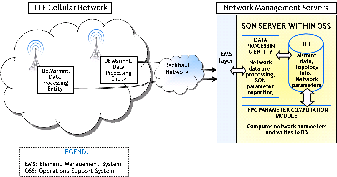
Figure 2: Underlying computation architecture.

Underlying Self-Optimized Networking (SON) architecture: The underlying SON architecture is shown in Figure 2. In this architecture, network monitoring happens in a distributed manner across the radio access network, and the heavy duty algorithmic computations happen centrally at the Network Management Servers. As opposed to a fully distributed (across eNBs) computation approach, this kind of hybrid SON architecture is the preferred by many operators for complex SON use-cases [1, 2] for two key reasons: capability to work across base stations from different vendors as is typically the case, and not having to deal with convergence issues of distributed schemes (due to asynchrony and message latency). We note two relevant aspects of this architecture:

• Main building blocks: The main building blocks are the following: (i) monitoring components at the cells that collect network measurements, appropriately process them to create Key Performance Indicators (KPIs), and communicate the measurement and KPIs to the central server, and (ii) the algorithmic computation engine (cloud servers) at a central server that makes use of the KPIs and compute the SON parameters that are then fed back to the network.

• Time-scale of computation: The KPIs from the network are typically communicated periodically. The period should be such that, it is short enough to capture the changing network dynamics that call for network re-configuration and is long enough for accurate estimation the relevant statistics. In general, most networks have periodic measurement reports with frequency $5\--15$ mins [30] but much faster minimization of drive test (MDT) data and UE trace information can be collected. In addition, measurement reports can be trigerred by events like traffic load above a certain threshold beyond normal.

Design questions: Given this architecture, to periodically compute the FPC-$\alpha$ parameters to maximize the network performance in the uplink, we need to answer two questions:

• Q1: What are the minimal set of network measurements required to configure FPC-$\alpha$ parameters?

• Q2: Based on these measurements, how should we choose $\alpha$, $P^{(0)}$ and average interference threshold for every cell ? The algorithms should be scalable and capable of updating the parameters as new measurement data arrives.

In Section V, we answer Q1 and propose a measurement based optimization framework , and in Section VI-VII , we develop learning based algorithms to answer Q2.

V Measurement and Optimization Framework

V-A Network Measurement Data

Additional notations: We will derive an expression of SINR of a typical uplink UE. Towards this goal, consider a network snapshot with a collection of UEs ${\mathcal{U}}$; a generic UE is indexed by $u\in{\mathcal{U}}$. Let ${\mathcal{U}}_{c}$ denote the set of UEs associated with cell-$c$. Denote by $l_{c}^{(u)}$ path loss from $u\in{\mathcal{U}}_{c}$ to its serving cell $c$. We also drop the superscript for UE and write $L_{c}$ to denote the path loss of a random UE associated with cell-$c$. We denote the mean path loss from a UE $u\in{\mathcal{U}}_{e}$ to an cell $c\in{\mathcal{J}}_{e}$ by $l_{e\rightarrow c}^{(u)}$. We also drop the superscript for UE and write $L_{e\rightarrow c}$ to denote the path loss from cell-$e$ to cell-$c$ of a random UE belonging to cell-$e$. These notations are also shown in Table I.

Remark 2 (Fast-fading and frequency selectivity).

All path loss variables must be interpreted in “time-average” sense so that the effect of fast-fading is averaged out. Indeed, fast-fading happens at a much faster time-scale (ms) than the FPC-$\alpha$ parameter computation time-scale of minutes. Also, SC-FDMA equalization at the receiver averages out the effect of frequency selectivity in an RB.

Expression for SINR: Consider a UE-$u$ that transmits to its serving cell-$c$ over the RBs assigned to it. Consider the transmission over any one RB that is assigned subcarriers in the set $S$ by the MAC scheduler. To derive the SINR over $S$, we wish to quantify the interference experienced by the received signal at serving cell-$c$ over $S$. Due to our observations on frequency hopping, the subcarriers within $S$ can be used in a neighboring cell by at most one UE. Note that, depending on the load on a cell, a RB may only be utilized only during a certain fraction of the transmission subframes. With this motivation, we define the following binary random variable:

$$O_{e\rightarrow c}\stackrel{{\scriptstyle\triangle}}{{=}}\left\{\begin{array}[]{lc}1&\begin{array}[]{c}\text{\small if cell-$e$ schedules a UE over the }\\ \text{\small resource block $S$ also used at cell-$c$}\end{array}\\ 0&\text{\small else}\end{array}\ \right.$$ (2)

In the above, we assume that $O_{e\rightarrow c}$ does not depend on the specific choice of $S$ and has identical distribution for all $S$. Denoting by $v$ the UE that occupies $S$ at cell-$e$, ignoring fast-fading, the interfering signal at serving cell-$c$ of UE-$u$ for transmissions over $S$ in cell-$e$ can be expressed as follows.

$$I_{e\rightarrow c} =O_{e\rightarrow c}P^{Tx}_{(v)}\ .\ l_{e\rightarrow c}^{(v)}=O_{e\rightarrow c}P^{(0)}_{e}(l_{e}^{(v)})^{\alpha_{e}}(l_{e\rightarrow c}^{(v)})^{-1}$$

It is instructive to note that, even without fluctuations due to fast fading, the interference $I_{e\rightarrow c}$ is random because the interfering UE-$v$ transmitting over $S$ in cell-$e$ could be any random UE in cell-$c$. In other words, the quantities $l_{e}^{(v)},l_{e\rightarrow c}^{(v)}$ can be viewed as a random sample from the joint distribution of $(L_{e},L_{e\rightarrow c})$. Thus the total interference at cell-$c$ over frequency block $S$ is a random variable $I_{c}$ given by

$$I_{c}=\sum_{e\in{\mathcal{J}}}O_{e\rightarrow c}P^{(0)}_{e}(L_{e})^{\alpha_{e}}(L_{e\rightarrow c})^{-1}$$ (3)

where we drop the superscript of the loss variables to mean that the loss is from a random UE in an interfering cell using the RB-$S$. This randomness is induced by MAC scheduling of the interfering cell. Now, the SINR of UE-$u$ in cell-$c$ denoted by $\mathsf{SINR}(l_{c}^{(u)})$ (as a function of UE-$u$’s path loss $l_{c}^{(u)}$) over RB-$S$ can be expressed as

$$\mathsf{SINR}(l_{c}^{(u)})=\frac{P^{Rx}_{(u)}}{I_{c}+N_{0}}$$

$$=\frac{P^{(0)}_{c}(l_{c}^{(u)})^{-(1-\alpha_{c})}}{\sum_{e\in{\mathcal{J}}_{c}}O_{e\rightarrow c}P^{(0)}_{e}(L_{e})^{\alpha}(L_{e\rightarrow c})^{-1}+N_{0}}$$ (4)

Measurement variables: It follows from (4) that, for any given $l_{c}^{(u)}$, $\mathsf{SINR}(l_{c}^{(u)})$ is a random variable that is fully characterized by the following distributions: joint distribution of $(L_{e},L_{e\rightarrow c})$ and $O_{e\rightarrow c}$ for all $e\in{\mathcal{J}}_{c}$. Furthermore, as we argue formally in Section V-B, towards computing an “average” network wide performance metric over the SON computation period, we also require $\rho_{c}$ the mean uplink load in cell-$c$ and path loss distribution $L_{c}$. The dependence on traffic load on the average network performance is also quite intuitive. We thus have the following.

Design of Measurement Statistics: For a given set of values of $P^{(0)}_{c},\alpha_{c}$, under FPC-$\alpha$ mechanism, any expected network wide performance metric can be fully characterized by the following statistics: 1. Joint path loss distribution $(L_{e},L_{e\rightarrow c})$ of uplink UEs for every interfering cell $e$ of $c$. 2. $\Pr(O_{e\rightarrow c}=1)$ which is the probability that cell-$e$ schedules a UE interfering with cell-$c$ for transmission over an RB. 3. Mean number of active uplink UEs (uplink load) in every cell-$c$ denoted by $\rho_{c}$. 4. Path loss distribution of uplink UEs of cell-$c$ denoted by $L_{c}$.

Histogram construction: The required distributions can be estimated using standard histogram inference techniques [9] using the following steps we state for completeness:

1. Collecting UE measurement samples: Since UE measurement reports contain reference signal strength (termed RSRP) from multiple neighboring cells, the RSRP values can be coverted into path losses using knowledge of cell transmit power. Thus, for a UE associated with cell-$c$, if a measurement report contains RSRP from cell-$c$ and cell-$e$ both, then it provides samples for $L_{c},$ and $(L_{e},L_{e\rightarrow c})$.

2. Binning the path loss data: This is a standard step where the range of $L_{c}$ and $(L_{e},L_{e\rightarrow c})$ are divided into several disjoint histogram bins and each data point is binned appropriately.

3. Estimating the occupancy probabilities $\Pr(O_{e\rightarrow c}=1)$: Assuming proportional-fair MAC scheduling where all UEs in a cell use the radio resources uniformly, $\Pr(O_{e\rightarrow c}=1)$ can be estimated as the fraction of UEs in cell-$e$ that interfere with cell-$c$. This estimation can be performed by simply computing the fraction of UEs in cell-$e$ that report measurements from cell-$c$.

We make two observations. First, the histograms are best maintained in dB scale to so that the range of path loss values is not too large. Second, in practice, the data samples for constructing the histograms can come for a large enough random subset of all the data.

V-B The IoT Control Problem in LTE HTNs

We are now formulate our problem based on the measurement histograms described in the previous section.

Network wide performance metric: Given our model, a suitable performance metric should satisfy two properties: (i) it should account for the randomness in the SINR’s in a meaningful manner, and (ii) it should strike a balance between aggregate cell throughputs and fairness.

We wish to propose a average performance metric where average is over all UE path losses that can realize the measurement data. Towards this end, we first define a performance metric for a typical UE-$u$ in cell-$c$ who has path loss to its serving cell given by $l_{c}^{(u)}$. Denote by $\gamma_{c}(l_{c}^{(u)})$ as the expected log-SINR of a typical UE-$u$ in cell-$c$, i.e., $\gamma_{c}(l_{c}^{(u)})={\mathbb{E}}[\ln\mathsf{SINR}(l_{c}^{(u)})]$ where the expression of $\mathsf{SINR}(l_{c}^{(u)})$ is given by (4). We now define the UE utility function $V(.)$ as follows:

$$V(\gamma_{c}(l_{c}^{(u)}))\stackrel{{\scriptstyle\triangle}}{{=}}\left\{\begin{array}[]{c}\text{\small Utility of a UE-$u$ in cell-$c$ as a }\\ \text{\small function of $\gamma_{c}(l_{c}^{(u)})={\mathbb{E}}[\ln\mathsf{SINR}(l_{c}^{(u)})]$}\end{array}\right\}$$ (5)

Here $V(.)$ is a concave increasing function and we have explicitly shown the SINR depends on the path loss $l_{c}^{(u)}$. Choosing the utility as a function of ${\mathbb{E}}[\ln\mathsf{SINR}_{u}]$ has two benefits. Firstly, $\ln(\mathsf{SINR}_{u})$ is a measure of the data rate with $\mathsf{SINR}_{u}$. Secondly, converting the SINR into a log-scale makes the problem tractable since it is well known that feasible power region is log-convex [35], and thus, we can use elements of convex optimization theory.

Having defined a utility for a typical UE, we are now in a position to define network wide performance metric obtained by averaging over all UE path losses that can realize the measurement data. We need additional notations for the histogram of $L_{c}$’s. Suppose the path loss histogram of $L_{c}$ is divided into $k$ disjoint intervals with mid-point of the intervals given by $l_{c}(1),l_{c}(2),\ldots,l_{c}(k_{c})$. Suppose in cell-$c$, the empirical probability of items in histogram bin-$b$ is given by $p_{c}(b)$. Then, we define the overall system utility as the expected utility of all UEs in all the cells where the expectation is over empirical path loss distribution given by the measurement data. This utility, as a function of vector of $P^{(0)}_{c},\alpha_{c}$’s (denoted by ${\mathbf{P}^{(0)}},\boldsymbol{\alpha}$) is given by.

$$\text{Util}({\mathbf{P}^{(0)}},\boldsymbol{\alpha})=\sum_{c\in{\mathcal{C}}}{\mathbb{E}}[\text{Total utility of UEs in cell-$c$}]$$

$$=\sum_{c\in{\mathcal{C}}}\sum_{b=1}^{k_{c}}{\mathbb{E}}[\text{Total utility of UE with path loss $l_{c}(b)$ in cell-$c$}]$$

$$=\sum_{c\in{\mathcal{C}}}\sum_{b=1}^{k_{c}}{\mathbb{E}}[\text{{\small Num. UEs with path loss $l_{c}(b)$}}]\times V(\gamma_{c}(l_{c}(b)))$$

$$=\sum_{c\in{\mathcal{C}}}\sum_{b=1}^{k_{c}}\rho_{c}\ p_{c}(b)\ V\left(\gamma_{c}(l_{c}(b))\right)$$ (6)

where $\gamma_{c}(l_{c}(b))$ is the expected SINR in log-scale for any UE with path loss $l_{c}(b)$ to its serving eNB of cell-$c$. The last step follows because the expected number of UEs with path loss $l_{c}(b)$ is product of expected number of UEs in cell-$c$ and the probability of a UE with path loss $l_{c}(b)$.

Choice of UE-utility: Though our techniques work for a generic concave and increasing $V(.)$, for our design and evaluation, we use the following form of $V(.)$ in the rest of paper:

$$V(\gamma)=\ln\ln(1+\exp(\gamma))\ .$$ (7)

One can verify that the function $V(.)$ defined above is concave. Roughly speaking, $\ln(1+\exp(\gamma))$ is the Shannon data rate corresponding to log-scale (natural log) SINR of $\gamma$. It is well known that utility defined by log of data rate strikes the right balance between fairness and overall system performance.

Remark 3 (Data rate and throughput).

In this paper, we use UE data rate or PHY data rate (in bits/sec/Hz) instead of UE throughputs (bits/sec/Hz). Under proportional-fair MAC scheduling, the dominant scheduling policy in LTE, UE throughput $R_{u}$ of UE-$u$ in cell-$c$, is roughly related to PHY data rate $r_{u}$ of UE-$u$ by $R_{u}=r_{u}/N_{c}$; here $N_{c}$ is the average number of simultaneously active users in cell-$c$. Thus, $\ln R_{u}=\ln r_{u}-\ln N_{c}$. In other words, the log of throughput and log of data rate are off by an additive constant independent of power control parameters.

We also observe that optimizing the total log-data rate of all UEs is aligned with the MAC objective of proportional-fair scheduling in LTE.

Measurement based IoT Control Problem (IoTC): We now formulate the problem of optimally configuring the parameters of the FPC-$\alpha$. This problem is commonly referred to as the Interference over Thermal (IoT) control problem because the optimal choice of $P^{(0)}_{c},\alpha_{c}$’s result in a suitable interference threshold above the noise floor in every cell. The problem can be succinctly stated as follows:

Given the path loss histograms of $L_{c},(L_{e},L_{e\rightarrow c})$, empirical distribution $O_{e\rightarrow c}$, and average traffic load $\rho_{c}$ at every cell-$c$, find optimal $P^{(0)}_{c},\alpha_{c}$ for every cell-$c$ such that we maximize $\text{Util}({\mathbf{P}^{(0)}},\boldsymbol{\alpha})$ given by (6).

At a first glance, the above problem may look complex due to the fact that $\text{Util}({\mathbf{P}^{(0)}},\boldsymbol{\alpha})$ is a function of several random variables. We will first formulate this problem as a mathematical program so that the problem becomes tractable. By using motivation from [35], we convert all powers, and path losses to logarithmic scale as follows.

$$\theta_{c}={\mathbb{E}}\left[\ln\left({\sum_{e\in{\mathcal{J}}_{c}}O_{e\rightarrow c}P^{(0)}_{e}(L_{e})^{\alpha}(L_{e\rightarrow c})^{-1}+N_{0}}\right)\right]$$ (8)

$$\pi_{c}=\ln P^{(0)}_{c}\ ,\ \lambda_{c}(b)=\ln l_{c}(b)\ ,\ \lambda_{ec}(b)=\ln l_{ec}(b)\ ,$$ (9)

$$\ \Lambda_{c}=\ln L_{c}\ ,\ \Lambda_{e\rightarrow c}=\ln L_{e\rightarrow c}$$ (10)

The notations are also shown in Table I. We can now re-write $\gamma_{c}(l_{c}(b))$ (given by (4)) in terms of these above variables as

$$\gamma_{c}(l_{c}(b))=\pi_{c}-(1-\alpha_{c})\lambda_{c}(b)-\theta_{c}$$ (11)

where,

$$\ \theta_{c}={\mathbb{E}}\left[\ln\left(\sum_{e\in{\mathcal{J}}_{c}}O_{e\rightarrow c}e^{(\pi_{e}+\alpha_{e}\Lambda_{e}-\Lambda_{e\rightarrow c})}+N_{0}\right)\right]$$ (12)

which has the standard look of SINR expression in log-scale. Thus, we can state the problem of maximizing $\text{Util}({\mathbf{P}^{(0)}},\boldsymbol{\alpha})$ as the problem of maximizing

$$\sum_{c}\sum_{b}\rho_{c}p_{c}(b)V(\gamma_{c}(l_{c}(b)))$$

subject to equality constraints given by (11) and (12). It turns out that the equality constraints can be re-written as inequalities to convert this into convex non-linear program (NLP) with inequality constraints. This leads to the following proposition where we have also imposed an upper bound on the maximum transmit power per RB and maximum average interference cap.

Proposition V.1.

Given measurement statistics of $L_{c},(L_{c},L_{e\rightarrow c}),O_{c}$ and average traffic load $\rho_{c}$ at every cell-$c$, the problem of maximizing $\text{Util}({\mathbf{P}^{(0)}},\boldsymbol{\alpha})$ given by (6), subject to maximum transmit power constraint on RB, is equivalent to the following convex program:

IoTC-SCP: $\displaystyle\max_{\{\pi_{c}\},\{\alpha_{c}\},\{\gamma_{c}(b)\}}\ \ \sum_{c,b}\rho_{c}p_{c}(b)V(\gamma_{c}(b))$ subject to, $\displaystyle\ \forall\ c\in{\mathcal{C}},b\in[1,k_{c}]:\ \gamma_{c}(b)\leq\pi_{c}-(1-\alpha_{c})\lambda_{c}(b)-\theta_{c}$ (13) $\displaystyle\ \forall\ c\in{\mathcal{C}}:\ \theta_{c}\geq{\mathbb{E}}\left[\ln\left(\sum_{e\in{\mathcal{J}}_{c}}O_{e\rightarrow c}e^{(\pi_{e}+\alpha_{e}\Lambda_{e}-\Lambda_{e\rightarrow c})}+N_{0}\right)\right]$ (14) $\displaystyle\ \forall\ c\in{\mathcal{C}},b\in[1,k_{c}]:\ \pi_{c}+\alpha_{c}\lambda_{c}(b)\leq\ln P_{max}$ (15) $\displaystyle\ \alpha_{c}\in[0,1],\ \gamma_{c}(b)\in[\gamma_{min},\infty),\ \ \theta_{c}\in[\ln N_{0},\ln I_{max}]$ (16)

Proof.

(Outline) First, at optimality, all of the inequalities must be met with equality from basic principles. Secondly, the constraint set is a convex region since the constraints (14) is convex due to convexity of LSE function [21]. ∎

We make two important remarks.

Remark 4 (IoTC-SCP constraints).

In IoTC-SCP, constraint (13) states that the expected SINR in log-scale can be no more than the receiver UE power less the expected uplink interference at the eNB, constraint (14) states that the expected interference at each cell has to be at least the expected sum of interferences from the neighboring cells, and constraint (15) limits the maximum power allowed per RB. Finally,  (16) states the valid domain of the variables $\alpha_{c},\theta_{c}$’s and $\gamma_{u}$’s, where, $\gamma_{min}$ is the minimum decodable SINR. Note that the valid domain of $\theta_{c}$ is $[\ln N_{0},\ln I_{max}]$ because maximum average interference in cells could need a cap due to hardware design constraints.

Remark 5 (Setting SINR target of UEs).

In IoT-SCP, suppose $\pi_{c}^{*},\alpha_{c}^{*},\theta_{c}^{*}$ represent the optimal values for cell-$c$ and let $P_{c}^{(0)*}=\exp(\pi_{c}^{*}),I_{c}^{*}=\exp(\theta_{c}^{*})$ be the optimal values in linear scale. Then, the SINR target of an arbitrary UE in cell-$c$ with average path loss $l_{c}^{(u)}$ is set as

$$\mathsf{SINR}_{\text{target}}(l_{c}^{(u)})=\frac{\min\left[P_{\max}\ (l_{c}^{(u)})^{-1},\ P_{c}^{(0)*}\ (l_{c}^{(u)})^{-(1-\alpha^{*}_{c})}\right]}{I_{c}^{*}}\ .$$ (17)

Challenges in solving IoTC-SCP: IoTC-SCP is somewhat different from a traditional non-linear program that are solved using standard gradient based approaches (using Lagrangian). The main challenge in solving IoTC-SCP comes from the randomness in the interferers. As a consequence of this, the expected value of r.h.s. of interference constraint (14) is computationally-intensive even for given values of the $\pi_{c}$’s and $\alpha_{c}$’s. Indeed, this requires accounting for $O(B_{max}^{K})$ number of interferer combination per cell where $B_{max}$ is the maximum number of histogram-bins of the joint distribution of $(L_{e},L_{e\rightarrow c})$ in any cell and $K$ is the maximum number of interferes of an cell. Repeating this computation for every iteration of a gradient based algorithm is next to impossible.

By adapting elements of learning theory, we propose two algorithms that strike a different performance-computation trade-off. One is optimal requiring more computational resources and the other is an approximate heuristic with fast computation times.

VI A Stochastic Learning Based Algorithm

We now develop a stochastic-learning based gradient algorithm.

We introduce additional notations for ease of exposition. Denote the original optimization variables $(\gamma_{c}(b),\pi_{c},\alpha_{c})$’s by the vector ${\mathbf{z}}$ (also called primal variables). We also denote the constraint set of the problem IoTC-SCP by the random function $h({\mathbf{z}},{\boldsymbol{O},\Lambda})$, i.e.

$$h({\mathbf{z}},{\boldsymbol{O},\Lambda})$$

$$=\left[\begin{array}[]{c}\left[\gamma_{c}(b)-\pi_{c}-(1-\alpha_{c})\lambda_{c}(b)\right]_{c\in{\mathcal{C}},b\in[1,k_{c}]}\\ \left[\ln\left(\sum_{e\in{\mathcal{J}}_{c}}O_{e\rightarrow c}e^{(\pi_{e}+\alpha_{e}\Lambda_{e}-\Lambda_{e\rightarrow c})}+N_{0}\right)-\theta_{c}\right]_{c\in{\mathcal{C}}}\\ \left[\pi_{c}+\alpha_{c}\lambda_{c}(b)-\ln P_{max}\right]_{c\in{\mathcal{C}},b\in[1,k_{c}]}\end{array}\right]$$ (21)

Thus, the IoTC-SCP problem can be simply stated as

$$\max_{{\mathbf{z}}}\sum_{c,b}V(\gamma_{c}(b))\ \ \text{s.t.}\ \ {\mathbb{E}}[h({\mathbf{z}},{\boldsymbol{O},\Lambda})]\leq 0\ .$$

In the above, the expectation is with respect to the random variables $O_{e\rightarrow c}$’s and $(\Lambda_{e},\Lambda_{e\rightarrow c})$’s. We define the random Lagrangian function as follows:

$${\mathcal{L}}({\boldsymbol{z}},h({\mathbf{z}},{\boldsymbol{O}},{\boldsymbol{\Lambda}}),{\mathbf{p}})=\sum_{u}V(\gamma_{u})-{\mathbf{p}}^{t}h({\mathbf{z}},{\mathbf{O}},{\boldsymbol{\Lambda}})$$ (22)

where, ${\mathbf{p}}\geq 0$ denotes the so called Lagrange multiplier vector and it has the same dimension as the number of constraints. Since the objective function of IoTC-SCP is concave and the constraint set is convex, one can readily show from convex optimization theory that [8]

OPT $$=\max_{{\mathbf{z}}}\min_{{\mathbf{p}}\geq 0}{\mathbb{E}}[{\mathcal{L}}({\boldsymbol{z}},h({\mathbf{z}},{\boldsymbol{O},\Lambda}),{\mathbf{p}})]$$ (23)

$$=\min_{{\mathbf{p}}\geq 0}\max_{{\mathbf{z}}}{\mathbb{E}}[{\mathcal{L}}({\boldsymbol{z}},h({\mathbf{z}},{\boldsymbol{O},\Lambda}),{\mathbf{p}})]\ ,$$

where OPT denotes the optimal value of IoTC-SCP. Our goal is to solve the IoTC-SCP problem by tackling the saddle point problem (23).

Useful bounds on the optimization variables: Before we describe our algorithm, we derive trivial but useful bounds on feasible primal variables. The iterative scheme to be described shortly projects the updates primal variables within these bounds. The proof is straightforward and skipped for want of space.

Lemma VI.1.

Any feasible $\gamma_{c}(b)$ and $\pi_{c}$ of the problem IoTC-SCP satisfies

$$\pi_{\min}\leq\pi_{c}\leq\pi_{\max},\ \ \gamma_{\min}\leq\gamma_{c}(b)\leq\gamma_{\max}\ ,$$

where,

$$\pi_{\max}=\ln P_{\max},\ \pi_{\min}=\gamma_{\min}+N_{0},\ \gamma_{\max}=\ln P_{\max}-N_{0}\ .$$

Intuition and a stochastic iterative algorithm: The equivalent problem (23) is referred to as the saddle point problem and one could use standard primal-dual techniques to solve this problem [29]. In such an approach, the primal variables and dual variables are updated alternatively in an iterative fashion, and each update uses a gradient (of ${\mathbb{E}}[{\mathcal{L}}(.)]$) ascent for the primal variables and gradient descent for the dual variables. However, computing the expectation and its gradient is computationally expensive (can be $O(B_{max}^{K})$ where $B_{max}$ is maximum histogram bins and $K$ is maximum number of interferers) and this has to be done in every iteration which is practically impossible. Instead, we perform primal-dual iterations by substituting the random variables with random samples of the random variables in every iteration: thus expectation computation is replaced by a procedure to draw a random sample from the histograms which is a computationally light procedure. The idea of replacing a random variable by a sample in an iterative scheme is not new, the entire field of stochastic approximation theory deals with such schemes and conditions for this to work [11]. Our contribution is in applying this powerful technique to the IoTC-SCP problem. By using elements of stochastic approximation theory, we also show that the resulting output converges to optimal.

We now describe our algorithm. Denote the value of the primal variables in iteration-$n$ by ${\mathbf{z}}_{n}$ and the value of the dual variables in iteration-$n$ by ${\mathbf{p}}_{n}$. We also denote by $\hat{{\mathbf{z}}}_{n}$ and $\hat{{\mathbf{p}}}_{n}$ the iteration average of the primal and dual variables respectively. The overall algorithm is summarized in Algorithm 1 and is described as follows:

Initialization: First ${\mathbf{z}}_{n},{\mathbf{p}}_{n},\hat{{\mathbf{z}}}_{n},\hat{{\mathbf{p}}}_{n}$ are initialized to positive values within bounds specified by Lemma VI.1.

Iterative steps: Denote by $a_{n}=1/n^{\zeta},0.5<\zeta\leq 1$ as the step size in iteration-$n$. The following steps are repeated for $n=0,1,2,\ldots$:

• Random Sampling of Interferers: This step is performed for each interfering cell pair $(c,e)$. For each cell-$e\in{\mathcal{J}}_{c}$ the following steps are performed:

  • Toss a coin with probability of head $\Pr(O_{e\rightarrow c}=1)$. Denote the outcome of this coin-toss by the $0\--1$ variable $\chi_{ec}$ where $\chi_{ec}$ takes value one if there is a head.

  • If $\chi_{ec}=1$, then draw a random sample from the joint distribution of $(L_{e},L_{e\rightarrow c})$ based on the histogram of this joint distribution. Denote the random sample, which is a 2-tuple by $(sa[1],sa[2])$. Let $(\xi_{ec}[1],\xi_{ec}[2])$ denote the logarithm of this random sample, i.e., $\xi_{ec}[i]=\ln(sa[i]),i=1,2\ .$

  • In the function $h(.)$ given by (21) representing the constraints of IoTC-SCP, replace the random variables $(\Lambda_{e},\Lambda_{e\rightarrow c})$ by the random sample $(\xi_{e}c[1],\xi_{ec}[2])$.

  Denote by ${\boldsymbol{\chi}},{\boldsymbol{\xi}}$ as the vector of $\chi_{ec},\xi_{ec}$’s samples. We write $h({\mathbf{z}}_{n},{\boldsymbol{\chi}},{\boldsymbol{\xi}}),{\mathbf{p}}_{n})$ as a function of these random samples along with the primal and dual variables in iteration-$n$.

• Primal Update: The primal variables are updated as

  $${\mathbf{z}}_{n+1}={\mathbf{z}}_{n}+a_{n}\nabla_{{\mathbf{z}}}{\mathcal{L}}({\mathbf{z}}_{n},h({\mathbf{z}}_{n},{\boldsymbol{\chi}},{\boldsymbol{\xi}}),{\mathbf{p}}_{n})$$ (24)

  where $\nabla_{{\mathbf{z}}}{\mathcal{L}}(.)$ denotes the partial derivative of ${\mathcal{L}}(.)$ with respect to ${\mathbf{z}}$.

      Next project updated values of $\alpha_{e},\pi_{e},\theta_{e},\gamma_{u}$’s respectively within intervals $[0,1]$, $[\pi_{\min},\pi_{\max}]$, $[\ln N_{0},\ln I_{max}]$,$[\gamma_{\min},\gamma_{\max}]$. For example, if the value of $\alpha_{e}$ in iteration-$(n+1)$, $({\alpha_{e}})_{n+1}>1$, then set $({\alpha_{e}})_{n+1}\leftarrow 1$; and, if any $({\alpha_{e}})_{n+1}<0$ set $({\alpha_{e}})_{n+1}\leftarrow 0$.

• Dual update: The dual variables are updated as

  $${\mathbf{p}}_{n+1}=\left[{\mathbf{p}}_{n}+a_{n}h({\mathbf{z}}_{n},{\boldsymbol{\chi}},{\boldsymbol{\xi}})\right]^{+}\ .$$ (25)

• Updating average iterates: The current value of the solution is given by average iterates

  $$\hat{{\mathbf{z}}}_{n+1} \leftarrow{\textstyle{\frac{1}{n}}}{\mathbf{z}}_{n}+(1-{\textstyle{\frac{1}{n}}})\hat{{\mathbf{z}}}_{n}$$

  $$\hat{{\mathbf{p}}}_{n+1} \leftarrow{\textstyle{\frac{1}{n}}}{\mathbf{p}}_{n}+(1-{\textstyle{\frac{1}{n}}})\hat{{\mathbf{p}}}_{n}\ .$$

The iterative steps are repeated for $N_{iter}$ iterations based on whether $\hat{{\mathbf{z}}}_{N_{iter}},\hat{{\mathbf{p}}}_{N_{iter}}$ converge within a desirable precision. There are many techniques are testing the convergence of stochastic iterations [5] that can be readily used for our purpose. The step-sizes $a_{n}$ can be set as $1/n^{\zeta},0.5<\zeta\leq 1$ or in an adaptive manner to speed up the convergence [20].

Algorithm 1 IoTC-SL: Stochastic Primal Dual Algorithm for IoTC Control.

1:  Initialize the primal variables to ${\mathbf{z}}_{0}$ and the dual variables to ${\mathbf{p}}_{0}.$

2:  for iterations $n=1$ to $n=N_{it}$ do

3:    For each interfering cell pair $(e,c)$ draw a random path loss sample from the joint distribution histogram of $(L_{e},L_{e\rightarrow c})$ and the replace the path loss random variables by these samples in the expression of $h(.)$ in (21).

4:    Update the primal variables according to gradient ascent based update rule in (24).

5:    Update the dual variables according to gradient descent based update rule in (25).

6:    Maintain average of the primal and dual variables over all the iterations

7:  end for

8:  The average of the primal variables over all the iterations is the output.

Asymptotic Optimality of Algorithm IoTC-SL We will now state the main analytical result for Algorithm IoTC-SL. The following result shows that the iterates generated by Algorithm IoTC-SCP converge to the optimal solution for “almost” every sample path of the iterates.

Theorem 1.

Suppose ${\mathbf{z}}^{*}$ is the optimal solution of IoTC-SCP. Then, the following holds:

$${\mathbf{z}}_{n}\rightarrow{\mathbf{z}}^{*}\ \ \text{with probability}\ 1\ .$$

Proof.

See Appendix. ∎

VII Regression Based Certainty Equivalent Heuristic

For ease of exposition, we re-write the random interference in constraint (14) of IoTC-SCP which is

$$\forall\ c\in{\mathcal{C}}:\ \theta_{c}\geq{\mathbb{E}}\left[\ln\left(\sum_{e\in{\mathcal{J}}_{c}}O_{e\rightarrow c}e^{(\pi_{e}+\alpha_{e}\Lambda_{e}-\Lambda_{e\rightarrow c})}+N_{0}\right)\right]\ .$$ (26)

The basic idea of this heuristic consists of two high-level methods. First is the notion of certainty equivalence where we replace the random log-interference by log of expected interference in (26) such that any solution with this modified constraint is a feasible solution of IoTC-SCP. Second is the notion of regression, where, using a known parametric distribution as model for the path loss statistics, we perform a fitting of the distribution parameters using the measurement data. Now the problem can be shown to be a standard non-linear program (NLP) that can be solved using off-the-self NLP solvers. We next explain the different steps.

Certainty equivalent approximation: We approximate the random interference constraint (26) as follows:

$$\forall\ c\in{\mathcal{C}}:\ \theta_{c}\geq\ln\left(\sum_{e\in{\mathcal{J}}_{c}}{\mathbb{E}}\left[O_{e\rightarrow c}e^{(\pi_{e}+\alpha_{e}\Lambda_{e}-\Lambda_{e\rightarrow c})}+N_{0}\right]\right)\ .$$ (27)

We now make a very important observation. Denote by $F_{approx}$ the feasible solution region of the optimization problem obtained by the above modification (27) of interference constraint (14) in IoTC-SCP. If $F_{IoTC-SCP}$ is the feasible region of IoTC-SCP, then it can be shown from Jensen’s inequality that $(\ref{eqn:ce1})\Rightarrow(\ref{eqn:reintcon})$, and thus,

$$F_{approx}\subseteq F_{IoTC-SCP}\ .$$

This means, if we replace constraint (26) by (27), we will produce feasible solution to IoTC-SCP.

Denoting $a_{e\rightarrow c}={\mathbb{E}}[O_{e\rightarrow c}]$, (27) can be rewritten as

$$\theta_{c}\geq\ln\left(\sum_{e\in{\mathcal{J}}_{c}}a_{e\rightarrow c}g(P^{(0)}_{e},\alpha_{e})+N_{0}\right)\ ,$$ (28)

where

$$g(\pi_{e},\alpha_{e})={\mathbb{E}}[e^{(\pi_{e}+\alpha_{e}\Lambda_{e}-\Lambda_{e\rightarrow c})}]\ .$$ (29)

Model for path losses: To simplify the r.h.s. of  (27), we use the following widely used path-loss model:

Distribution Model for Path loss: For each interfering cell pair, $(c,e)$, the joint distribution of the random variables $(L_{e},L_{e\rightarrow c})$ are log-normal. In other words, the distribution of $(\Lambda_{e},\Lambda_{e\rightarrow c})=(\ln L_{e},\ln L_{e\rightarrow c})$ is jointly Normal.

Indeed, log-normal distribution is a very reasonable statistical model for spatial path loss distribution [22]. For ease of exposition, we define the following two dimensional vectors:

$${\mathbf{Z}}_{ec}=\left[\begin{array}[]{c}\Lambda_{e}\\ \Lambda_{e\rightarrow c}\end{array}\right],\ \ \beta_{e}=\left[\begin{array}[]{c}\alpha_{e}\\ -1\end{array}\right],\ \$$ (30)

${\mathbf{Z}}_{ec}$ is defined for each interfering cell pair $(c,e)$ and $\beta_{e}$ for each cell $e$. Note that, under our modeling assumption, the random variable ${\mathbf{Z}}_{ec}$ is bi-variate jointly Normal random variable. The parameters of ${\mathbf{Z}}_{ec}$ are defined by the following mean and correlation matrix:

$${\mathbf{m}}_{ec}={\mathbb{E}}[{\mathbf{Z}}_{ec}]\ ,\ {\mathbf{C}}_{ec}={\mathbb{E}}[({\mathbf{Z}}_{ec}-{\mathbf{m}}_{e})({\mathbf{Z}}_{ec}-{\mathbf{m}}_{e})^{t}]$$ (31)

Note that ${\mathbf{m}}_{ec}$ is a $2\times 1$ vector and ${\mathbf{C}}_{ec}$ is a $2\times 2$ symmetric positive definite matrix. Also, ${\mathbf{m}}_{ec},{\mathbf{C}}_{ec}$ are model parameters that can be estimated from the measurement data using standard techniques for Gaussian parameter estimation [25] (also outlined in Algorithm 2).

Model based simplification of IoTC-SCP: Using the definition of ${\mathbf{Z}}_{ce}$ in (30), we can rewrite $g(\pi_{e},\alpha_{e})$ in (29) as follows.

$$g(\pi_{e},\alpha_{e})={\mathbb{E}}[\exp(\pi_{e}+\beta_{e}^{t}{\mathbf{Z}}_{ec})]$$

Since ${\mathbf{Z}}_{ec}$ is Normal, the above expression can be simplified using moment generating functions of multivariate Normal random variables as [25]:

$$\hat{g}(\pi_{e},\alpha_{e})=\exp\left(\pi_{e}+\beta_{e}^{t}{\mathbf{m}}_{e}+{\textstyle{\frac{1}{2}}}\beta_{e}^{t}{\mathbf{C}}_{ec}\beta_{e}\right)$$ (32)

where we write $\hat{g}(.)$ to mean that it is an estimate of $g(.)$ under the assumed statistical model of path losses. We can now solve the following modified version of IoTC-SCP problem where we replace the interference constraint (14) by

$$I_{c}\geq\ln\left(\sum_{e\in{\mathcal{J}}_{c}}a_{e\rightarrow c}\hat{g}(\pi_{e},\alpha_{e})+N_{0}\right).$$

This is stated as follows:

IoTC-CE: $\displaystyle\max_{\{\pi_{e}\},\{\alpha_{e}\},\{\gamma_{c}(b)\}}\sum_{c,b}\rho_{c}p_{c}(b)V(\gamma_{c}(b))$ subject to, $\displaystyle\ \ \ \gamma_{c}(b)\leq\pi_{c}-(1-\alpha_{c})\lambda_{c}(b)-\theta_{c}$ $\displaystyle\ \ \ \theta_{c}\geq\ln\left[\sum_{e\in{\mathcal{J}}_{c}}a_{e\rightarrow c}e^{(\pi_{e}+\beta_{e}^{t}{\mathbf{m}}_{ec}+{\textstyle{\frac{1}{2}}}\beta_{e}^{t}{\mathbf{C}}_{ec}\beta_{e})}+N_{0}\right]$ $\displaystyle\ \ \ \pi_{c}+\alpha_{c}\lambda_{c}(b)\leq\ln P_{max}$ $\displaystyle\ \ \ \alpha_{c}\in[0,1],\ \theta_{c}\in[\ln N_{0},\ln I_{max}],\ \gamma_{c}(b)\in[\gamma_{min},\infty)$

Algorithm 2 SolveIoTC-CE: Regression based deterministic heuristic for IoTC COntrol.

1:  Regression step: For each interfering cell pair $(e,c)$, we use the path-loss measurements to find a normal fit of the Gaussian random random variable ${\mathbf{Z}}_{ec}$ given by (30). Suppose the histogram bins based on the measurement of joint distribution of $(L_{e},L_{e\rightarrow c})$ are indexed by $b$ where $b=1,2,\ldots$. Suppose bin-$b$ represents the values $(l_{e}(b),l_{e\rightarrow c}(b))$ and has empirical probability mass $p_{{ec}}(b)$. Let $(\lambda_{e},\lambda_{e\rightarrow c})=(\ln l_{e}(b),\ln l_{e\rightarrow c}(b))$. Then a maximum-likelihood estimator [25] of ${\mathbf{m}}_{ec},{\mathbf{C}}_{ec}$ is as follows:

$${\mathbf{m}}_{ec}=\left[\begin{array}[]{c}\sum_{b}p_{ec}(b)\lambda_{e}(b)\\ \sum_{b}p_{ec}(b)\lambda_{e\rightarrow c}(b)\end{array}\right],\ {\mathbf{C}}_{ec}=\left[\begin{array}[]{cc}\hat{\sigma_{e}^{2}}&\hat{\sigma_{ec}^{2}}\\ \hat{\sigma_{ec}^{2}}&\hat{\sigma_{e}^{2}}\end{array}\right]$$

where,

$$\hat{\sigma_{e}^{2}} =\sum_{b}p_{ec}(b)(\lambda_{e}(b)-{\mathbf{m}}_{ec}[1])^{2}$$

$$\hat{\sigma_{ec}^{2}} =\sum_{b}p_{ec}(b)(\lambda_{e}(b)-{\mathbf{m}}_{ec}[1])(\lambda_{e\rightarrow c}(b)-{\mathbf{m}}_{ec}[2])$$

2:  Deterministic non-linear program solving: With the above estimates, we solve the NLP given by IoTC-CE using standard tools for solving deterministic non-linear programs (such as, dual based techniques, primal-dual techniques etc.) [7].

IoTC-CE is convex deterministic NLP (and hence standard tools of solving NLP can be used), provided the function $\hat{g}(\pi_{e},\alpha_{e}))$ is convex in $(\pi_{e},\beta_{e})$. The following lemma shows shows that $\hat{g}(\pi_{e},\alpha_{e}))$ is indeed a convex function.

Lemma VII.1.

The function $\ln(\sum_{e\in{\mathcal{J}}_{c}}\hat{g}(\pi_{e},\alpha_{e})+N_{0})$ is convex in $\pi_{e}$ and $\alpha_{e}$. Thus IoTC-CE is a convex NLP.

Proof.

Since convex and component-wise increasing function of a vector of convex functions is convex [8], the result follows. The details are omitted for want of space. ∎

Overall algorithm by putting it all together: As outlined in Algorithm 2, we have two steps. First we use the measurement data to estimate the parameter-matrices ${\mathbf{m}}_{e},{\mathbf{C}}_{ec}$ of the distribution ${\mathbf{Z}}_{ce}$. Second, we use these values to solve IoTC-CE using standard NLP solving techniques.

The main benefit of the approach in this section is that, it is computationally not so intensive and can be solved using powerful commercial NLP solvers; the price we pay is the sub-optimality.

VIII Evaluation using Propagation Map from a Real LTE Deployment

The primary goal of our evaluation is two fold. First, to understand the gains provided by LeAP as compared to other popular approaches. Second, to understand the effect of important design parameters like histogram bin-size and IoT-cap on LeAP performance. In addition, we also provide a comparison of the two proposed LeAP algorithms.

VIII-A Evaluation Platform

Evaluation platform: For our evaluation purpose, we implemented the following components in Figure 2: SQL database (DB) that saves network information, the data access layer which interacts with the DB and creates the measurement data discussed in Section V, and the IoT-control parameter ($P^{(0)},\alpha$’s) computation engine. All our implementations were based on .NET using C# and are multi-threaded using the Task Parallelization Library (TPL) facilities. We implemented Algorithm 1 within our framework using suitable data structures to enable multi-threaded implementation. We skip these implementation details for want of space. For network measurement information saved in the DB, we used real signal propagation map from an actual deployment but synthetic mobile locations generated using a commercial network planning tool in a manner described shortly.

Note that, in our evaluation platform, we have not yet implemented Algorithm 2. Such implementation requires integrating a .NET compatible commercial NLP solver within our architecture, a feature that is in progress. However, just for the purpose of comparison, we have developed a stand-alone implementation of Algorithm 2 using CVX [15] a free NLP Matlab solver. This can operate only on moderate sized networks with restricted objective function forms and is very slow for practical needs.

VIII-B Evaluation Setup and Methodology

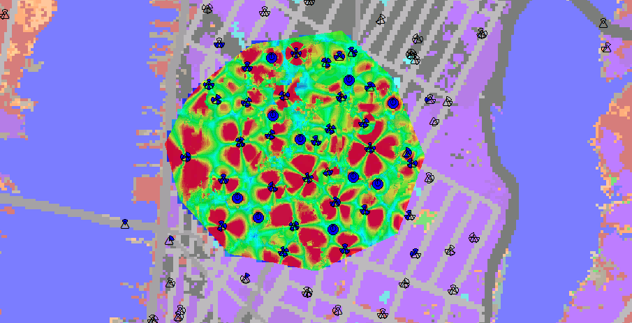
Figure 3: LTE signal map in evaluated section of a major US metro. The heat map is based on downlink SINR as the uplink SINR depends on specific FPC scheme.

We used signals propagation maps generated by a real operational LTE network in a major US metro area (see Figure 3 for the propagation heat map). The terrain category, cell site locations, and drive-test propagation data from the network were fed into a commercially available Radio Network Planning (RNP) tool that is used by operators for cellular planing [4]. The carrier bandwidth is 10 MHz in the 700 MHz LTE band. There is no dependency of LeAP design to the specific tool used for evaluation purpose.

For our evaluation, we selected an area of around 9 $\text{km}^{2}$ in the central business district of the city with 115 macro cells. This part of the city has a very high density of macro cells due to high volume of mobile data-traffic. Going forward, LTE deployments are going to have low-power pico cells in addition to high power macro cells. Since picos are not yet deployed in reality, 10 pico locations were manually embedded into the network planning tool using its built-in capabilities. Macros have transmit power 40 W and picos have transmit power 4 W. All including, we have 125 cells in the evaluated topology.

Though we had propagation data based on a real deployment, we do not have access to actual mobile measurements at this stage. To generate measurement data required for our evaluation, we generated synthetic mobile locations using the capabilities of RNP tool. These location were used to generate measurement data as follows:

1. Using the drive-test calibrated data, terrain information and statistical channel models, the RNP tool was used to generate signal propagation matrix in every pixel in the area of interest in a major US metro as shown in Figure 3.

2. The RNP tool was then used to drop thousands of UEs in several locations where the density of dropped UEs was as per dense-urban density (450 active mobile per sq-km). In addition, we defined mobile hotspots around some of the picos where the mobile density was doubled. Based on the signal propagation matrix in every pixel and mobile drop locations, the RNP tool readily generated all path loss data from UEs to it serving cell and neighboring cells and also mobile to cell association matrix.

3. The mobile path loss data was used to generate the histograms and the other measurement KPIs proposed in Section V. This data was then fed into LeAP database.

Once the measurement data is available, the results were generated as follows:

1. The measurement data from LeAP database was read by our implementation of LeAP algorithm that generated the cell power control parameters.

2. To evaluate the gains, the parameters generated by LeAP algorithm (or any other comparative algorithm) were evaluated for a random UE snapshot generated by RNP tool where each UE’s data-rate based on its SINR-target given by (17) was computed.

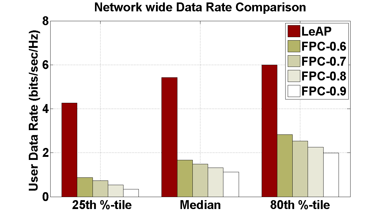
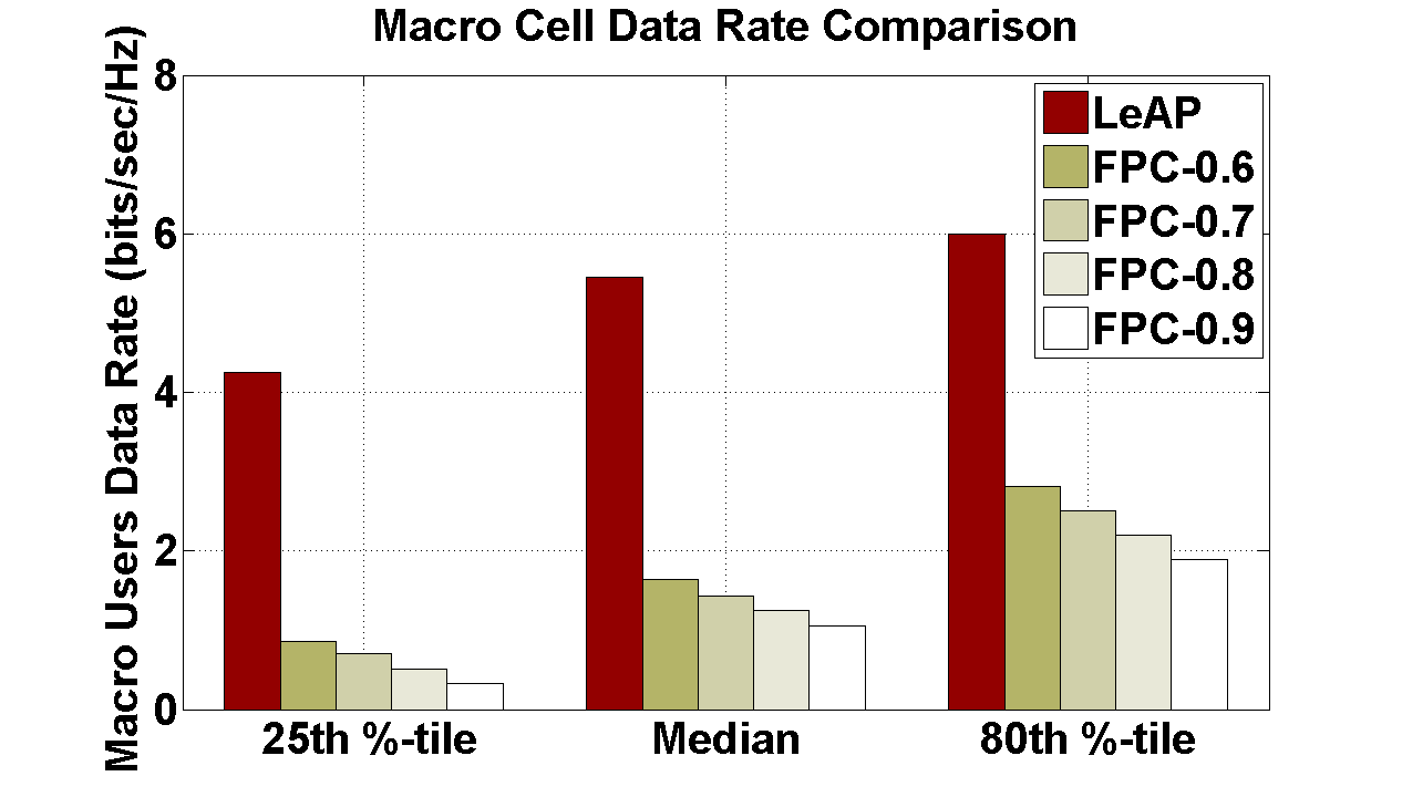
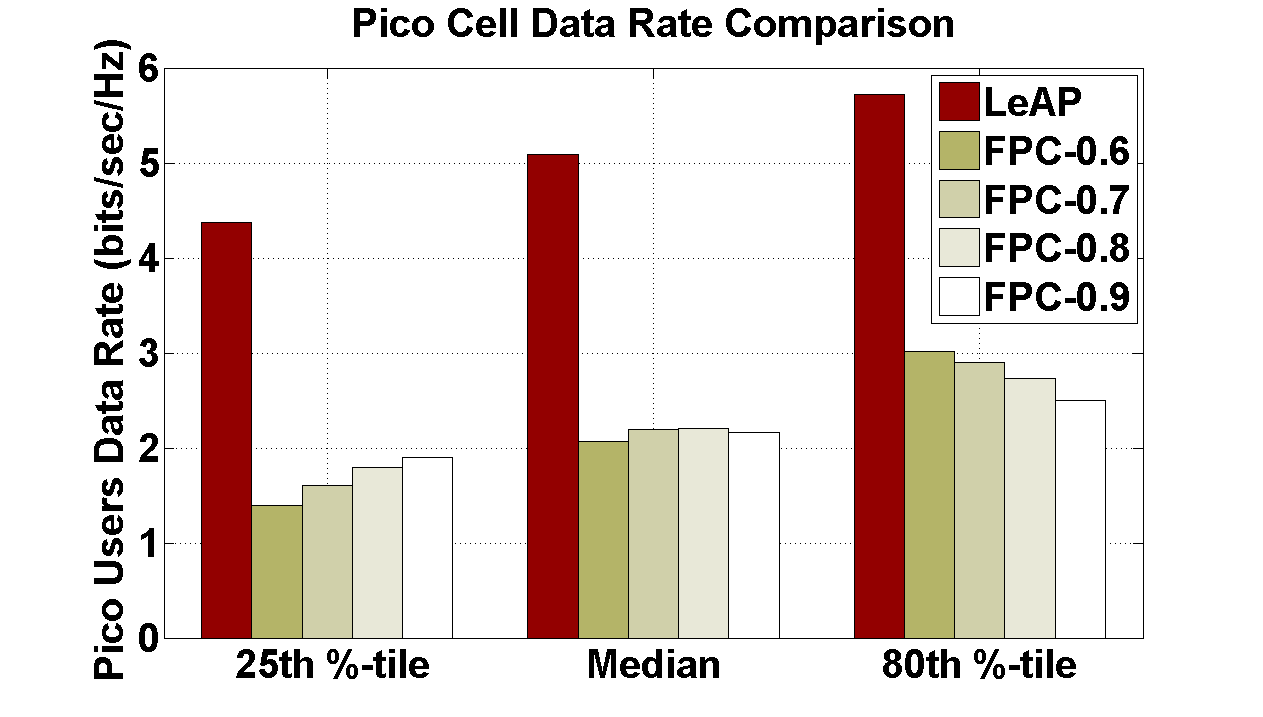
Figure 4: LeAP performance gain over fixed-$\alpha$ FPC for (a) all UEs, (b) macro cell UEs, and (c) pico cell UEs.

Comparative schemes and LeAP parameters: We compared the following schemes for our evaluation:

1) LeAP Algorithm: For most of our evaluation, we use Algorithm 1 which has provable guarantees at a small expense of computation time. Algorithm 2 requires expensive off-the-shelf non-linear solver for large scale networks. Nevertheless, we show the performance of Algorithm 2 using a free solver based stand-alone implementation.

2) Fixed-${\boldsymbol{\alpha}}$ FPC (FA-FPC): We compare the performance of LeAP with the following approach popular in literature [6, 17]: fix the same value of $\alpha$ (typically $\alpha=0.8$) for all cells and set $P^{(0)}$ so that every mobile’s SINR is above the decoding threshold. SINR computation is performed using a nominal value of interference $I_{nominal}$ that is typically $5\--15$ dB above the noise floor.

There are two important design parameters for LeAP: the histogram bin-size and the IoT-cap, that is partly dictated by hardware designs constraints. In our evaluation, default choice of bin-size is 1 dB and the default IoT-cap is 20 dB. In our problem framework (see IoTC-SCP), we set

$$I_{max}=\text{IoT-cap}-2.\text{bin-size}$$

as a design choice to provide cushion for the path loss error introduced by histogram binning. We also show results by varying the bin-size and IoT-cap. Also, $P_{max}=100$ mW/RB.

VIII-C Results

LeAP Performance Gains: In this section we evaluate the performance of LeAP at various quantiles of the user data rate CDF produced across the population of the users in our deployment area. Figure 4 shows the LeAP performance with FA-FPC for all users, users that are associated with macro cells, and users that are associated with pico cells. Our main observations are as follows:

• As seen in Figure 4 LeAP provides a data rate improvement over the best FA-FPC scheme, of $4.9\times,3.25\times,2.12\times$ for the $20^{th},50^{th},80^{th}$ %-tile respectively. In other words, with LeAP, at least half the users see a data rate improvement at least $3\times$ and 80% of the users see an improvement of at least $2\times$. The larger gain at lower percentiles indicate that LeAP is really beneficial to users towards the cell edge who are most affected by inter-cell interference.

• As seen in Figure 4,  4, LeAP provides higher improvement to macro users as compared to pico users. The median improvement of pico users’ data rate is $2.3\times$ whereas it is $3.3\times$ for macro users. This can be explained by the fact that the macros use high power and have larger coverage leading to more users affected by inter-cell interference and thus more users can reap the benefits of LeAP.

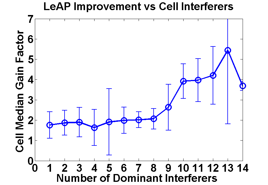
Figure 5: Cell-wise LeAP gain vs. number of interferers.

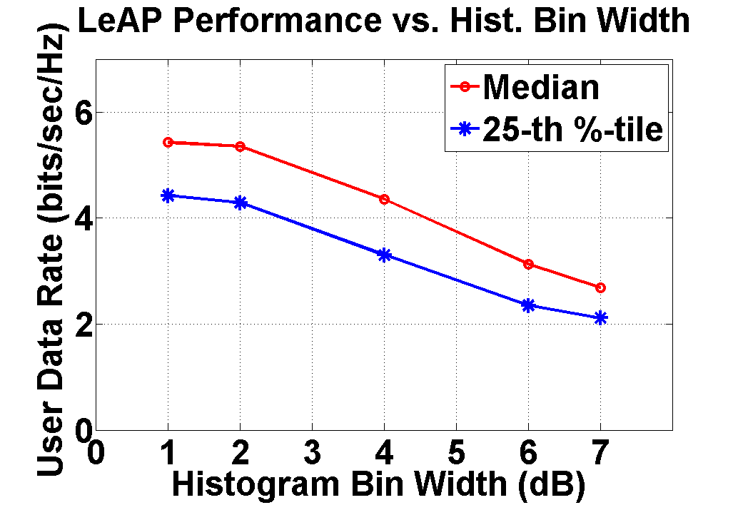
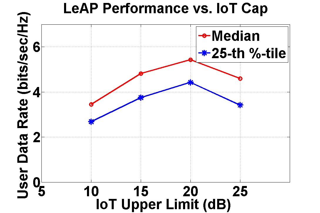
Figure 6: Effect of (a) histogram bin size on median LeAP performance, and (b) effect of IoT-cap on median LeAP performance.

In Figure 5, we show the gains of different cells in the network by grouping all the 125 cells based on number of dominant interferers. An interfering cell is dominant at least $5\%$ of its uplink users, the users that selected this cell as serving, that can interfere, i.e., $\Pr(\text{interference})\geq 0.05.$. Figure 5 shows that the typical median data rate gain of cell-groups with 8 or fewer interferers is around $2\times$ whereas, the gains are around $4\times$ for cell-groups with more than 10 interferers. We also show error bar for each cell group based on the sample standard deviation of gains within each group. We remark that the plot shows irregularity at 13 and 14 interferers due to having just 3 cells with 13-14 interferers. These results suggest LeAP and other SON algorithms need not be applied uniformly across the network but only in the interference problematic regions of the network. Identifying these regions from measurement data is an interesting problem outside the scope of this paper.

LeAP performance with variation of histogram bin-size and IoT-cap: In Figure 6, we show the median performance gains of LeAP by varying histogram bin-size, with IoT-cap either fixed at 20 dB or varying (with bin-size fixed at 2 dB) . Our main observations are as follows:

• Effect of bin-size: From Figure 6 we see that the performance of LeAP and the gains deteriorate with larger histogram bin-size which is intuitive. However, there is marginal performance loss for 2 dB bin-size as compared to 1 dB bin-size, but the performance deteriorates considerably for 6 dB bin-size. This suggests that the right bin-size should not exceed $2$ dB for optimal LeAP performance.

• Effect of IoT-cap: The performance of LeAP with IoT-cap is shown in Figure 6. Till an IoT-cap of around 20 dB, the median performance improves with increase in $I_{max}$ as there is greater flexibility in optimization. Past that, the gain decreases as can be seen with an IoT-cap of 25 dB. This behavior is intriguing and can be explained as follows. Let $I_{actual}$ be the actual interference in the network for given user location. Also, $I_{max}$ is the maximum interference in IoT-SCP problem formulation. Note that, $I_{actual}$ could be higher than $I_{max}$ due to approximations introduced by histogram binning. Intuitively, with larger $I_{max}$, the gap between $I_{actual}$ and $I_{max}$ is larger as there are more interfering cells with non-negligible interference signal. Thus, beyond a point, the binning approximations somewhat nullify the benefits of increase in $I_{max}$.

LeAP computation times: For the 125 cell network, Algorithm 1 showed excellent gains after running for $50,000$ iterations. Using a 3.4 GHz Intel Xeon CPU with 16 GB RAM on a 6 core machine with 64 bit OS, the running times of our multi-threaded implementation were on an average 12 sec with a variability of around 5 sec. Since we expect the periodicity of measurement reports to be in minutes, this shows the scalability of our design.

Comparison of IoTC-CE and IoTC-SL: We also have developed a stand-alone implementation of IoTC-CE algorithm using a open source NLP solver called CVX [15]. CVX is a powerful tool for moderate sized problems that can deal with the constraints in the IoTC-CE problem, that involve log-sum-exponential functions. However, CVX cannot operate for 125 cells in our evaluation network due to associated variable limits in the solver, and so we choose a sub-region consisting of 35 cells including 4 pico cells. Furthermore, since CVX only takes objective functions of certain forms, we modified our objective by choosing utility as $V(\gamma)=\ln(\mathsf{SINR}_{\min}+\ln(\exp(\gamma)))$, clearly an approximation.

In Figure 7, we compare the median data rate of the two LeAP algorithms and the best FPC scheme in our evaluation. IoTC-CE still provides $90\%$ improvement for all cells and around $2\times$ improvements for macro cells. For pico cells, IoTC-CE outperforms IoTC-SL. Also, the performance of median data rate of IoTC-CE is $36\%$ less compared to IoTC-SL. This could be partially due to that the approximated $V(.)$ worsens at lower SINR.

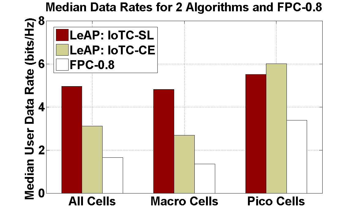
Figure 7: Median data rate comparison for IoTC-CE and IoTC-SL. Histogram bin width is $0.5$ dB.

IX Concluding Remarks

In this work we have proposed LeAP, a measurement data driven approach for optimizing uplink performance in an LTE network. Using propagation data from a real operational LTE network, we show the huge gains to be had using our approach.

Appendix A Two Simple Useful Lemmas

We will need the following inequalities in our proof. The proofs of the inequalities are there in a longer version of the paper.

Lemma A.1.

The following holds for $a_{0}=1$ and real $a_{i}>0,i=1,2,\ldots,k$:

$$\ln^{2}(\sum_{i=0}^{k}e^{a_{i}})\leq\ln^{2}(k+1)+(1+2\ln(k+1))\sum_{i=0}^{k}a_{i}^{2}\ .$$

Lemma A.2.

For real positive $x_{1},x_{2}$, the following holds:

$$\ln^{2}(x_{1}+x_{2})\leq\ln^{2}(e+x_{1}+x_{2})+\ln^{2}x_{2}\ .$$

Appendix B Proof of Theorem 1

We will use results from stochastic approximation theory to prove our results. Broadly speaking, stochastic approximation theory states that, under suitable conditions, discrete iterations with random variables converge to an equilibrium point of an equivalent deterministic ODE (ordinary differential equation) [11]. In other words, to show that a discrete-stochastic update rule converges to a desired point, we need to show the following steps [11]: (i) define an equivalent deterministic ODE, (ii) argue that the ODE has an equilibrium point identical to to the underlying discrete-stochastic update rule, and (iii) argue that conditions for limiting behavior of discrete-stochastic update rule to be similar to that of the ODE is satisfied (these conditions are provided by stochastic approximation theory).

Defining a limiting ODE: Let $m$ be the dimension of ${\mathbf{z}}$ or equivalently the number of primal variables. First, define the following operator $\Gamma_{{\mathbf{z}}}({\mathbf{y}})$ parametrized by primal variable ${\mathbf{z}}$:

$$\Gamma_{{\mathbf{z}}}({\mathbf{y}})=\left[\Gamma_{z_{1}}^{(1)}(y_{1})\ \ \Gamma_{z_{2}}^{(2)}(y_{2})\ldots\Gamma_{z_{m}}^{(m)}(y_{m})\ \ \ldots\right]^{t}\ ,$$

where

$$\Gamma_{z_{i}}^{(i)}(y_{i})=\left\{\begin{array}[]{cl}y_{i}{\mathbb{I}}_{\{y_{i}>0\}}&,\ \text{if}\ z_{i}=z_{i,\min}\\ y_{i}{\mathbb{I}}_{\{y_{i}<0\}}&,\ \text{if}\ z_{i}=z_{i,\max}\\ y_{i}&,\ \text{else}\end{array}\right.$$

In the above, $z_{i,\min}$ and $z_{i,\max}$ are the lower and the upper bounds of the corresponding primal variables. Similarly, define the functions $\Gamma_{{\mathbf{p}}}^{+}({\mathbf{q}})$ parametrized by ${\mathbf{p}}=[p_{1},\ p_{2},\ \ldots p_{n}]$ as

$$\Gamma^{+}_{{\mathbf{p}}}({\mathbf{q}}) =\left[\Gamma_{p_{1}}^{+}(q_{1})\ \ \Gamma_{p_{2}}^{+}(q_{2})\ \ldots\ \Gamma_{p_{n}}^{+}(q_{n})\right]$$

where,

$$\Gamma_{p_{j}}^{+}(q_{j}) =\left\{\begin{array}[]{cl}q_{j}{\mathbb{I}}_{\{q_{j}>0\}}&,\ \text{if}\ p_{j}=0\\ q_{j}&,\ \text{if}\ p_{j}>0\\ \end{array}\right.$$

We now define the following equivalent ODE for the iterative update rule in Algorithm IoTC-SDP.

$$\begin{bmatrix}{\mathbf{\dot{z}}}(t)\\ {\mathbf{\dot{p}}}(t)\end{bmatrix} =\begin{bmatrix}\Gamma_{{\mathbf{z}}(t)}\left({\mathbb{E}}[{{\mathcal{L}}}_{{\mathbf{z}}}({\mathbf{z}}(t),h({\mathbf{z}}(t),{\mathbf{O}},{\boldsymbol{\Lambda}}),{\mathbf{p}}(t))]\right)\\ \Gamma_{{\mathbf{p}}(t)}^{+}({\mathbb{E}}[h({\mathbf{z}}(t),{\mathbf{O}},{\boldsymbol{\Lambda}})])\end{bmatrix}$$

(33)

Asymptotic equivalence of ODE: The fundamental result in stochastic approximation theory [11] implies that the ODE defined in (33) has similar asymptotic behavior to the updates defined in Algorithm IoTC-SL provided certain conditions hold. The following lemma establishes this equivalence by verifying these conditions in our setup.

Lemma B.1.

The stochastic primal-dual update rule of Algorithm IoTC-SL given by (24) and (25) converges to the invariant set of ODE given by (33).

Proof.

We introduce some notations to start with. Rewrite the iterative update steps (24) and (25) in Algorithm IoTC-SL in a compact form as

$$\begin{bmatrix}{\mathbf{z}}_{n+1}\\ {\mathbf{p}}_{n+1}\end{bmatrix} ={\mathcal{P}}\left(\begin{bmatrix}{\mathbf{z}}_{n}\\ {\mathbf{p}}_{n}\end{bmatrix}+a_{n}M_{n}\right)$$

where,

$$M_{n}=\begin{bmatrix}\nabla_{{\mathbf{z}}}{\mathcal{L}}({\mathbf{z}}_{n},h({\mathbf{z}}_{n},{\boldsymbol{\chi}},{\boldsymbol{\xi}}),{\mathbf{p}}_{n})\\ h({\mathbf{z}}_{n},{\boldsymbol{\chi}},{\boldsymbol{\xi}})\end{bmatrix}$$ (34)

and ${\mathcal{P}}(.)$ denotes the projection of the primal variables into the compact set defined by bounds in Lemma VI.1 and dual variables into the positive axis.

According to Chapter 5.4 [11], the candidate equivalent ODE is given by

$$\begin{bmatrix}{\mathbf{\dot{z}}}(t)\\ {\mathbf{\dot{p}}}(t)\end{bmatrix} =\Gamma_{({\mathbf{z}}(t),{\mathbf{p}}(t))}\begin{bmatrix}\left({\mathbb{E}}[{{\mathcal{L}}}_{{\mathbf{z}}}({\mathbf{z}}(t),h({\mathbf{z}}(t),{\mathbf{O}},{\boldsymbol{\Lambda}}),{\mathbf{p}}(t))]\right)\\ {\mathbb{E}}[h({\mathbf{z}}(t),{\mathbf{O}},{\boldsymbol{\Lambda}})]\end{bmatrix}$$

where

$$\Gamma_{({\mathbf{x}})}({\mathbf{y}})=\lim_{\delta\downarrow 0}\frac{{\mathcal{P}}({\mathbf{x}}+\delta{\mathbf{y}})-{\mathcal{P}}({{\mathbf{y}}})}{\delta}\ .$$

One can verify that this candidate equivalent ODE is precisely the one defined by (33). Also, with a step-size of $a_{n}=1/n$, for iterative update steps (24) and (25) in Algorithm IoTC-SL to converge to an invariant set of the candidate ODE, we need to verify two conditions for our case (Chapter 5.4 [11]):

• C1: The functions, $\Gamma_{{\mathbf{z}}(t)}\left({\mathbb{E}}[{{\mathcal{L}}}_{{\mathbf{z}}}({\mathbf{z}},h({\mathbf{z}},{\mathbf{O}},{\boldsymbol{\Lambda}}),{\mathbf{p}})]\right)$ and $\Gamma_{{\mathbf{p}}}^{+}({\mathbb{E}}[h({\mathbf{z}},{\mathbf{O}},{\boldsymbol{\Lambda}}))$ are Lipschitz in ${\mathbf{z}}$ and ${\mathbf{p}}$.

• C2: The random variable $M_{n}$ satisfies

  $${\mathbb{E}}[{\|{M_{n}}\|}^{2}]\leq K(1+{\|{{\mathbf{z}}_{n}}\|}^{2}+{\|{{\mathbf{p}}_{n}}\|}^{2})$$

  for some constant $K>0$.

The conditions are not difficult to verify for our problem. We outline the steps in the following.

Verifying C1: We need to show the Lipschitz continuity of the r.h.s. of (33) in ${\mathbf{z}}$ and ${\mathbf{p}}$. First note that the ODE (33) is defined such that ${\mathbf{z}(t)},t\geq 0$ lies within the compact set defined in Lemma VI.1 (provided the initial conditions are also within that set) from which it follows that all terms (in the r.h.s. of  (33)) containing the primal variables are bounded. Also, the r.h.s of (33) is a linear function of the dual variables ${\mathbf{p}}$. One can combine these two facts and argue easily l.h.s. of (33) is Lipschitz in ${\mathbf{z}}$ and ${\mathbf{p}}$. We skip the details.

Verifying C2: Note from (21) that, the randomness in $h({\mathbf{z}}_{n},{\boldsymbol{\chi}},{\boldsymbol{\xi}})$ is only due to randomness in $Z_{c,n}$ where

$$Z_{c,n}=\ln\left(\sum_{e\in{\mathcal{J}}_{c}}\chi_{e}e^{(\pi_{e,n}+\alpha_{e,n}\xi_{e}-\xi_{e\rightarrow c})}+N_{0}\right).$$

We can use the boundedness of the primal variables ${\mathbf{z}}$ to show that

$${\mathbb{E}}[M_{n}^{2}]\leq K_{1}+\sum_{c\in{\mathcal{C}}}K_{2}{\mathbb{E}}[Z_{c,n}^{2}]\ ,$$ (35)

for suitable positive constants $K_{1}$ and $K_{2}$. To see this, first observe the following.

$${\mathbb{E}}[Z_{c,n}^{2}]$$

$$\leq{\mathbb{E}}\left[\ln^{2}\left(e+\sum_{e\in{\mathcal{J}}_{c}}\chi_{e}e^{(\pi_{e,n}+\alpha_{e,n}\xi_{e}-\xi_{e\rightarrow c})}+N_{0}\right)\right]+\ln^{2}N_{0}$$

where we have applied Lemma A.2. Define $A>1$ as the upper bound on the path loss in linear-scale in the entire network. Now notice that the function $f(x)=\ln^{2}(x+e)$ is concave for $x>0$. By applying Jensen’s inequality and definition of $A$,

$${\mathbb{E}}[Z_{c,n}^{2}]$$

$$\leq\ln^{2}\left(\sum_{e\in{\mathcal{J}}_{c}}{\mathbb{E}}\left[\chi_{e}e^{(\pi_{e,n}+\alpha_{e,n}\xi_{e}-\xi_{e\rightarrow c})}\right]+e+N_{0}\right)+\ln^{2}N_{0}$$

$$\leq\ln^{2}\left(A\sum_{e\in{\mathcal{J}}_{c}}e^{\pi_{e,n}}+e+N_{0}\right)+\ln^{2}N_{0}$$

Applying Lemma A.1 to the previous step, we have for suitable constants $K_{3}$ and $K_{4}$ (i.e., $K_{3},\ K_{4}$ are independent of $\pi_{e,n}$’s),

$${\mathbb{E}}[Z_{c,n}^{2}] \leq K_{3}+K_{4}\sum_{e\in{\mathcal{J}}_{c}}\ln^{2}(e^{\pi_{e,n}})=K_{3}+K_{4}\sum_{e\in{\mathcal{J}}_{c}}\pi^{2}_{e,n}$$

The above combined with (35) implies that,

$${\mathbb{E}}[M_{n}^{2}]\leq K_{5}+K_{6}{\|{{\boldsymbol{\pi}_{n}}}\|}^{2}$$

for system dependent constants $K_{5},K_{6}$ (i.e., $K_{5},\ K_{6}$ could depend on the network topology, but they are independent of the primal and dual variables). Condition C2 is thus verified.

The lemma is proved since we have verified C1 and C2. ∎

Global Stability of the ODE: Now that we have argued that Algorithm IoTC-SL behaves like the ODE (33) asymptotically, we prove that ODE (33) converges to the optimal point of problem IoTC-SCP.

Lemma B.2.

The ODE given by (33) is globally asymptotically stable and the system converges to saddle point solution of ${\mathcal{L}}({\mathbf{z}},{\mathbf{p}})$ which also corresponds to the optimai value of ${\mathbf{z}}$.

Proof.

Consider the Lyapunov function

$$W(t)={\|{{\mathbf{z}}(t)-{\mathbf{z}}^{*}}\|}^{2}+{\|{{\mathbf{p}}(t)-{\mathbf{p}}^{*}}\|}^{2}\ ,$$

where, ${{\mathbf{z}}}^{*}$ and ${{\mathbf{p}}}^{*}$ are the primal and dual optimal solution of the problem IoTC-SCP. Now note the following.

$$\dot{W}(t) =2({\mathbf{z}}(t)-{\mathbf{z}}^{*})^{t}\dot{{\mathbf{z}}}(t)+2({\mathbf{p}}(t)-{\mathbf{p}}^{*})^{t}\dot{{\mathbf{p}}}(t)$$

$$=2({\mathbf{z}}(t)-{\mathbf{z}}^{*})^{t}\Gamma_{{\mathbf{z}}(t)}\left({\mathbb{E}}[{{\mathcal{L}}}_{{\mathbf{z}}}({\mathbf{z}}(t),h({\mathbf{z}}(t),{\mathbf{O}},{\boldsymbol{\Lambda}}),{\mathbf{p}}(t))]\right)$$

$$\ \ +2({\mathbf{p}}(t)-{\mathbf{p}}^{*})^{t}\Gamma_{{\mathbf{p}}(t)}^{+}({\mathbb{E}}[h({\mathbf{z}}(t),{\mathbf{O}},{\boldsymbol{\Lambda}})])$$ (36)

Now note from the definition of $\Gamma_{{\mathbf{z}}}(.)$ that,

$$(z_{i}-z_{i}^{*})\Gamma_{z_{i}}^{(i)}(y_{i})\leq(z_{i}-z_{i}^{*})y_{i}\ ,$$

since $z_{i,\min}\leq z_{i}^{*}\leq z_{i,\max}$. Also,

$$(p_{i}-p_{i}^{*})\Gamma_{p_{i}}^{+}(q_{i})\leq(p_{i}-p_{i}^{*})q_{i}\ .$$

It thus follows from (36) that

$$\dot{W}(t)\leq 2({\mathbf{z}}(t)-{\mathbf{z}}^{*})^{t}{\mathbb{E}}[\nabla_{{\mathbf{z}}}{{\mathcal{L}}}({\mathbf{z}}(t),h({\mathbf{z}}(t),{\mathbf{O}},{\boldsymbol{\Lambda}}),{\mathbf{p}}(t))]$$

$$\ \ -2({\mathbf{p}}(t)-{\mathbf{p}}^{*})^{t}{\mathbb{E}}[\nabla_{{\mathbf{p}}}{\mathcal{L}}({\mathbf{z}}(t),h({\mathbf{z}}(t),{\mathbf{O}},{\boldsymbol{\Lambda}}),{\mathbf{p}}(t))]$$ (37)

For notational convenience, let $G(.)$ denote the function

$$G({\mathbf{z}},{\mathbf{p}})={\mathbb{E}}[{{\mathcal{L}}}({\mathbf{z}},h({\mathbf{z}},{\mathbf{O}},{\boldsymbol{\Lambda}}),{\mathbf{p}})]\ .$$

Note that $G({\mathbf{z}},{\mathbf{p}})$ is concave in ${\mathbf{z}}$ and convex in ${\mathbf{p}}$. Thus, from the proerty of convex and concave functions[8]

$$({\mathbf{z}}-{\mathbf{z}}^{*})^{t}\nabla_{{\mathbf{z}}}G({\mathbf{z}},{\mathbf{p}})\leq G({\mathbf{z}},{\mathbf{p}})-G({\mathbf{z}}^{*},{\mathbf{p}})$$

and

$$({\mathbf{p}}-{\mathbf{p}}^{*})^{t}\nabla_{{\mathbf{p}}}G({\mathbf{z}},{\mathbf{p}})\geq G({\mathbf{z}},{\mathbf{p}})-G({\mathbf{z}},{\mathbf{p}}^{*})\ ,$$

which applied to (37) implies

$$\dot{W}(t)$$

$$\leq G({\mathbf{z}}(t),{\mathbf{p}}(t))-G({\mathbf{z}}^{*},{\mathbf{p}}(t))-(G({\mathbf{z}}(t),{\mathbf{p}}(t))-G({\mathbf{z}}(t),{\mathbf{p}}^{*}))$$

$$=G({\mathbf{z}}(t),{\mathbf{p}}^{*})-G({\mathbf{z}}^{*},{\mathbf{p}}(t))$$ (38)

Since $({\mathbf{z}}^{*},{\mathbf{p}}^{*})$ is a saddle point solution of

$$\max_{{\mathbf{z}}}\min_{{\mathbf{p}}\geq 0}G({\mathbf{z}},{\mathbf{p}})=\min_{{\mathbf{p}}\geq 0}\max_{{\mathbf{z}}}G({\mathbf{z}},{\mathbf{p}})\ ,$$

we have, $G({\mathbf{z}},{\mathbf{p}}^{*})\leq G({\mathbf{z}}^{*},{\mathbf{p}}^{*})\leq G({\mathbf{z}}^{*},{\mathbf{p}})$ for any ${\mathbf{z}}$ and ${\mathbf{p}}\geq 0$, from which it follows that

$$\dot{W}(t)\leq 0\ ,$$

with equality iff ${\mathbf{z}}(t)={\mathbf{z}}^{*}$ and ${\mathbf{p}}(t)={\mathbf{p}}^{*}$. Thus, it follows from La’Salle’s invariance principle [26] that the ODE given by (33) converges to $({\mathbf{z}}^{*},{\mathbf{p}}^{*})$.

∎

Putting it all together: Proof of Theorem 1. Lemma B.1 shows that Algorithm IoTC-SL converges to the invaraint set of ODE (33) and Lemma B.2 shows that the ODE converges to the optimal point of problem IoTC-SCP. Thus Algorithm IoTC-SL converges to the optimal point of problem IoTC-SCP. Hence the proof.

References

- [1] http://www.sonlte.com/technology/.
- [2] http://lteworld.org/category/tags/son.
- [3] 3GPP Technical Specification 36.331. Available from www.3gpp.org.
- [4] Atoll 3.2, Radio Network Planning Tool. http://www.forsk.com/atoll/.
- [5] Alexopoulos, C. In Winter Simulation Conference.
- [6] Amirijoo, M., Jorguseski, L., Litjens, R., and Nascimento, R. Effectiveness of cell outage compensation in lte networks. In Consumer Communications and Networking Conference (CCNC), 2011 IEEE (2011), pp. 642-647.
- [7] Bertsekas, D. Nonlinear Programming. Athena Scientific, 1999.
- [8] Bertsekas, D., Nedic, A., and Ozdaglar, A. Convex Analysis and Optimization. Athena Scientific, 2003.
- [9] Bishop, C. M. Pattern Recognition and Machine Learning (Information Science and Statistics). Springer-Verlag New York, Inc., Secaucus, NJ, USA, 2006.
- [10] Boche, H., and Stanczak, S. Strict convexity of the feasible log-sir region. IEEE Transactions on Communications 56, 9 (2008), 1511-1518.
- [11] Borkar, V. Stochastic Approximation: A Dynamical Systems Viewpoint. Cambridge University Press, 2008.
- [12] Chiang, M., and Bell, J. Balancing supply and demand of bandwidth in wireless cellular networks: Utility maximization over powers and rates. In IEEE INFOCOM (2004).
- [13] Chiang, M., Hande, P., Lan, T., and Tan, C. W. Power Control in Wireless Cellular Networks Power Control in Wireless Cellular Networks: Foundation and Trends in Networking. now, 2008.
- [14] Coupechoux, M., and Kelif, J.-M. How to set the fractional power control compensation factor in lte ? In Sarnoff Symposium, 2011 34th IEEE (2011).
- [15] CVX Research, I. CVX: Matlab software for disciplined convex programming, version 2.0 beta. http://cvxr.com/cvx, Sep 2012.
- [16] Dahlman, E., Parkvall, S., Skold, J., and Beming, P. 3G Evolution: HSPA and LTE for Mobile Boradband. Academic Press, 2008.
- [17] et. al., C. U. C. Performance of Uplink Fractional Power Control in UTRAN LTE. In VTC Spring (2008), pp. 2517-2521.
- [18] et. al., M. B. Interference Based Power Control Performance in LTE Uplink. In Wireless Communication Systems. 2008. ISWCS ’08. IEEE International Symposium on (2008), pp. 698-702.
- [19] Foschini, G. J., and Miljanic, Z. A simple distributed autonomous power control algorithm and its convergence. Vehicular Tech., IEEE Trans. on 42, 4 (Nov 1993), 641-646.
- [20] George, A. P., and Powell, W. B. Adaptive stepsizes for recursive estimation with applications in approximate dynamic programming. Mach. Learn. 65, 1 (Oct 2006), 167–198.
- [21] Ghaoui, L. E. Hyper-Textbook: Optimization Models and Applications.
- [22] Goldsmith, A. Wireless Communications. Cambridge University Press, New York, NY, USA, 2005.
- [23] Hande, P., Rangan, S., Chiang, M., and Wu, X. Distributed uplink power control for optimal SOR assignment in cellular data networks. IEEE/ACM Trans. Netw. 16, 6 (2008), 1420-1433.
- [24] Hu, H., Zhang, J., Zheng, X., Yang, Y., and Wu, P. Self-configuration and self-optimization for LTE networks. Communications Magazine, IEEE 48, 2 (February), 94-100.
- [25] Kay, S. M. 1 ed. Apr.
- [26] Khalil, H. Nonlinear Systems. Prentice Hall, 2002.
- [27] Lobinger, A., Stefanski, S., Jansen, T., and Balan, I. Load balancing in downlink lte self-optimizing networks. In Vehicular Technology Conference (VTC 2010-Spring), 2010 IEEE 71st (May), pp. 1-5.
- [28] Madan, R., Borran, J., Sampath, A., Bhushan, N., Khandekar, A., and Ji, T. Cell association and interference coordination in heterogeneous lte-a cellular networks. IEEE Journal on Selected Areas in Communications 28 (2010), 1479–1489.
- [29] Nedic, A., and Ozdaglar, A. Subgradient methods for saddle-point problems. Journal of Optimization Theory and Applications (2009), 205-228.
- [30] Penttinen, J. T. J. The LTE/SAE Deployment Handbook. John Wiley & Sons, January 2012.
- [31] Rahman, M., Yanikomeroglu, H., and Wong, W. Enhancing cell-edge performance: a downlink dynamic interference avoidance scheme with inter-cell coordination. IEEE Transactions on Wireless Communications 9, 4 (2010), 1414–1425.
- [32] Saraydar, C., Mandayam, N. B., and Goodman, D. J. Pricing and power control in a multicell wireless data network. IEEE JOURNAL ON SELECTED AREAS IN COMMUNICATIONS 19 (2001), 1883–1892.
- [33] Son, H., Lee, S., Kim, S., and Shin, Y. Soft load balancing over heterogeneous wireless networks. Vehicular Technology, IEEE Transactions on 57, 4 (July), 2632-2638.
- [34] Stolyar, A., and Viswanathan, H. Self-organizing dynamic fractional frequency reuse in ofdma systems. In INFOCOM (2008), IEEE, pp. 691–699.
- [35] Sung, C. W. Log-convexity property of the feasible sir region in power-controlled cellular systems. IEEE Communications Letters 6, 6 (2002).
- [36] Turkka, J., Nihtila, T., and Viering, I. Performance of LTE son uplink load balancing in non-regular network. In Personal Indoor and Mobile Radio Communications (PIMRC), 2011 IEEE 22nd International Symposium on (Sept.).
- [37] Xiao, M., Shroff, N. B., and Chong, E. K. P. A utility-based power-control scheme in wireless cellular systems. IEEE/ACM TRANS. ON NETWORKING 11, 2 (2003), 210–221.
- [38] Yates, R. D. A framework for uplink power control in cellular radio systems. IEEE Journal on Selected Areas in Communications 13 (1996), 1341-1347.
- [39] Zhang, H., Prasad, N., Rangarajan, S., Mekhail, S., Said, S., and Arnott, R. Standards-compliant lte and lte-a uplink power control. In Communications (ICC), 2012 IEEE International Conference on (2012).