On the Relaxation Behaviors of Slow and Classical Glitches: Observational Biases and Their Opposite Recovery Trends

Abstract

We study the pulsar timing properties and the data analysis methods during glitch recoveries. In some cases one first fits the time-of-arrivals (TOAs) to obtain the “time-averaged” frequency $\nu$ and its first derivative $\dot{\nu}$, and then fits models to them. However, our simulations show that $\nu$ and $\dot{\nu}$ obtained this way are systematically biased, unless the time intervals between the nearby data points of TOAs are smaller than about $10^{4}$ s, which is much shorter than typical observation intervals. Alternatively, glitch parameters can be obtained by fitting the phases directly with relatively smaller biases; but the initial recovery timescale is usually chosen by eyes, which may introduce a strong bias. We also construct a phenomenological model by assuming a pulsar’s spin-down law of $\dot{\nu}\nu^{-3}=-H_{0}G(t)$ with $G(t)=1+\kappa e^{-t/\tau}$ for a glitch recovery, where $H_{0}$ is a constant and $\kappa$ and $\tau$ are the glitch parameters to be found. This model can reproduce the observed data of slow glitches from B1822–09 and a giant classical glitch of B2334+61, with $\kappa<0$ or $\kappa>0$, respectively. We then use this model to simulate TOA data and test several fitting procedures for a glitch recovery. The best procedure is: 1) use a very high order polynomial (e.g. to 50th order) to precisely describe the phase; 2) then obtain $\nu(t)$ and $\dot{\nu}(t)$ from the polynomial; and 3) the glitch parameters are obtained from $\nu(t)$ or $\dot{\nu}(t)$. Finally, the uncertainty in the starting time $t_{0}$ of a classical glitch causes uncertainties to some glitch parameters, but less so to a slow glitch and $t_{0}$ of which can be determined from data.

1 Introduction

Pulsars are very stable rotators. However, many pulsars exhibit significant timing irregularities, i.e., unpredicted arrival times of pulses. There are two main types of timing irregularities, namely ‘timing noise’ which is consisted of low-frequency quasi-periodic structures, and ‘glitches’ which are abrupt increases in their spin rates followed by relaxations.

Glitch activities are more frequent in relatively young pulsars with a characteristic age of $10^{4}-10^{5}$ yr (Shemar & Lyne 1996; Wang et al. 2000). For the hundreds of glitches observed, their typical fractional jumps in spin frequency $\nu$ are in the range of $\Delta\nu/\nu\approx 10^{-11}-10^{-5}$, and their relative increment in frequency derivative is $\Delta\dot{\nu}/\dot{\nu}\sim 10^{-3}$. Despite the abundance of observational data accumulated for over $40$ years, we are still far from satisfactory understanding of glitch events. Traditional models mainly involve the expected superfluid nature of part of the neutron star interior (Anderson & Itoh 1975; Ruderman 1976), and the angular momentum is carried in the form of microscopic, quantized vortices, whose density determines the rotation rate of a pulsar. Mostly, these vortices are pinned to the crust and the charged matter in the core of the star, thus their outward drifting motions are prevented (Anderson & Itoh 1975; Alpar 1977; Pines et al. 1980; Alpar et al. 1981; Anderson et al. 1982). However, as the crust spins down due to the electromagnetic braking, a rotational lag and stress (Magnus force) gradually builds up. A glitch occurs when the stress reaches some critical value and the pinning breaks, vortices suddenly move outward and impart their angular momentum to the crust. Immediately after the glitch, the vortices are pinned to other parts again and the superfluid is effectively decoupled from the crust.

Following the seminal work of Baym, Pethick & Pines (1969), there are two classes of models that have been developed to explore the dynamical evolution of pinned superfluid during the post-glitch recovery. One kind of models involve a weak coupling between the superfluid and the crust due to the interaction between free vortices and the coulomb lattice of nuclei (Jones 1990, 1992, 1998). Another kind of models assume that the vortices creep rate is highly temperature-dependent. As the vortices creep through the crust, angular momentum is gradually transferred (Alpar 1984a, 1984b; Link, Epstein & Baym 1993; Larson & Link 2002). Superfluid vortex dynamics can model the relaxation well; however, there are still many significant problems unsolved. For instance, the mechanism that triggers the glitch in the first place and the detailed processes of angular momentum transfer during the recovery are still controversial. It has been suggested that such an event may be triggered by large temperature perturbations (Link & Epstein 1996), or caused by starquakes (Baym & Pines 1971; Cheng et al. 1992), or the interactions of the proton vortices and the crustal magnetic field (Sedrakian & Cordes 1999), or the superfluid r-mode instability (Andersson, Comer, & Prix 2003; Glampedakis & Andersson 2009).

Very recently, Pizzochero (2011) proposed an analytic model for angular momentum transfer associated with Vela-like glitches for the storage and release of superfluid vorticity, and Seveso et al. (2012) and Haskell et al. (2013) extended the model to realistic equations of state and relativistic backgrounds. Haskell et al. (2012) further modeled all stages of Vela glitches with a two-fluid hydrodynamical approach. Furthermore, Haskell & Antonopoulou (2013) showed that if glitches are indeed due to large scale unpinning of superfluid vortices, the different regions in which the unpinning occurs and the respective timescales on which they recouple can lead to various observed jump and relaxation signatures. However, by combining the latest observational data for prolific glitching pulsars with theoretical results for the crust entrainment, Andersson et al. (2012) found that the required superfluid reservoir exceeds that available in the crust. Coincidentally, Chamel (2013) found that the glitches observed in the Vela pulsar require an additional reservoir of angular momentum, since the maximum amount of angular momentum that can possibly be transferred during glitches is severely limited by the non-dissipative entrainment effects. This challenges superfluid vortex model of the glitch phenomenon. Besides, some of the glitch events, such as those with persistent offset in the spin-down rate of the Crab pulsar following the 1975 glitch is difficult to explain with the dynamic coupling between the crust and the superfluid interior. An alternative explanation of the observed frequency deficit is an increase in the external torque caused by a rearrangement of the stellar magnetic field (Link 1992, 1998). Observationally, many pulsar phenomena, including the mode changing, pulsar-shape variability and spin-down rates switching, are caused by changes in pulsar’s magnetosphere (Lyne et al. 2010). Thus these relaxation processes may also be produced by the magnetosphere activities, which are induced by initial starquakes.

It has also been observed in recent years that some pulsars (e.g. PSR J1825-0935 and PSR J1835-1106) show another type of irregularity characterized by a gradual increase in $\nu$, accompanied by a rapid decrease in $|\dot{\nu}|$ and subsequent exponential increase back to its initial value (Zou et al. 2004; Shabanova 2005). That is the so-called ‘slow glitch’. Currently, there is still no convincing theoretical understanding for slow glitches. Peng & Xu (2008) proposed that, after a collapse or a small star-quake, the solid superficial layer of a rigid quark star may be heated and becomes a viscous fluid, which will eventually produce a gradual increase in $\nu$. However, Hobbs et al. (2010) and Lyne et al. (2010) argued that the slow glitches have the same origin as the timing noise of many pulsars.

For the recovery processes of both glitch and slow glitch events, the variations of spin frequency $\nu$ and its first derivative $\dot{\nu}$ of pulsars are obtained from polynomial fit results of arriving time epochs of pulses. The local TOAs of the mean pulses for individual observing sessions are determined from the maximum cross correlation between the observed mean pulses and a Gaussian profile template. The profile template is a mean pulse with high signal-to-noise ratio, obtained by summing the best-quality mean pulses over several observing sessions. Correction of TOAs to the solar system barycenter can be done using TEMPO2 program with the Jet Propulsion Laboratory DE405 ephemeris (Standish 1998). These TOAs are then weighted by the inverse squares of their estimated uncertainty. Since the rotational period is nearly constant, these observable quantities, $\nu$, $\dot{\nu}$ and $\ddot{\nu}$ can be obtained by fitting the phases to the third order of its Taylor expansion over a time span $t_{\rm s}$,

$$\Phi_{i}={\Phi}+\nu(t_{i}-t)+\frac{1}{2}\dot{\nu}(t_{i}-t)^{2}+\frac{1}{6}\ddot{\nu}(t_{i}-t)^{3}.$$ (1)

One can thus get the values of $\nu$, $\dot{\nu}$ and $\ddot{\nu}$ at $t$ from fitting to Equation (1) for independent $N$ data blocks around $t$, i.e. $i=1,...,N$. Apparently, these observational quantities obtained this way are not instantaneous results, rather, the “averaged” results over each data block (i.e. over each $t_{\rm s}$) and extrapolated to $t$, which are not necessarily the same as the instantaneous values (denoted as $\nu_{\rm I}$ and $\dot{\nu}_{\rm I}$). Thus, they are called “averaged” values (denoted as $\nu_{\rm A}$ and $\dot{\nu}_{\rm A}$) in this work. Usually, $t_{\rm s}$ is much less than pulsar’s spin-down age $\tau_{c}$, thus the differences between instantaneous values and “averaged” values are not significant, and consequently $\nu_{\rm A}$ and $\dot{\nu}_{\rm A}$ are good approximations for $\nu_{\rm I}$ and $\dot{\nu}_{\rm I}$ in most cases. However, it has been found recently that oscillations of the “apparent” magnetic fields of neutron stars are responsible for the observed signs and magnitudes of $\ddot{\nu}$, the second derivative of frequency, and braking indices (Biryukov et al. 2012; Pons et al. 2012; Zhang & Xie 2012a, 2012b). We further suggested that the oscillation time scales are between 10-100 yr, comparable to $t_{\rm s}$, thus making the fitted spin-down parameters different from the true and instantaneous spin-down parameters. Similarly, considerable biases may also exist when fitting the glitch recovery data, since the glitch recovery time scales are also comparable with $t_{\rm s}$.

In section 2, we simulate several pulsar timing data analysis procedures for glitch recoveries, and find that the glitch parameters, obtained from the averaged $\nu_{\rm A}$ and $\dot{\nu}_{\rm A}$, have significant systematic biases compared with that obtained with the instantaneous $\nu_{\rm I}$ and $\dot{\nu}_{\rm I}$. In order to get the true glitch parameters with the reported, yet averaged glitch recovery data $\nu_{\rm O}$ and $\dot{\nu_{\rm O}}$, a phenomenological or physical glitch model is needed to be combined with simulations. We thus present a phenomenological spin-down model during a glitch recovery, and model several slow glitch recovery events and the recovery of a giant classical glitch in section 3. In section 4, we test four fitting procedures based on the phenomenological spin-down model and find that the best method is taking a very high order polynomial to fit the phase and then taking its derivatives to obtain $\nu(t)$ and $\dot{\nu}(t)$. In Section 5, we discuss how to obtain the model parameters of glitch recoveries more accurately. The results are summarized in section 6.

2 Simulating Data Analysis of Glitch Recoveries

2.1 Simulation for $\dot{\nu}$-fitting procedure

By fitting the TOA set $\{\Phi(t_{i})\}$ to Equation (1), one can get $\{\nu(t)\}$ and $\{\dot{\nu}(t)\}$. When $\{\nu(t)\}$ and $\{\dot{\nu}(t)\}$ show exponential relaxations, their variations following the jump at epoch $t_{\rm 0}$ can be described as the following empirical functions (e.g. Yuan et al. 2010, Roy et al. 2012),

$$\nu(t)={\nu_{0}}(t)+\Delta\nu_{\rm p}+\Delta\dot{\nu}_{\rm p}\Delta t+\frac{1}{2}\Delta\ddot{\nu}_{\rm p}\Delta t^{2}+\sum_{j}\Delta\nu_{{\rm d}j}e^{-\Delta t/\tau_{j}},$$ (2)

and

$$\dot{\nu}(t)={\dot{\nu}_{0}}(t)+\Delta\dot{\nu}_{\rm p}+\Delta\ddot{\nu}_{\rm p}\Delta t+\sum_{j}\Delta\dot{\nu}_{{\rm d}j}e^{-\Delta t/\tau_{j}},$$ (3)

where $\Delta t=t-t_{\rm 0}$, $\Delta\nu_{\rm p}$ and $\Delta\dot{\nu}_{\rm p}$ are permanent changes in $\nu$ and $\dot{\nu}$ relative to the pre-glitch solution $\nu_{0}(t)$ and $\dot{\nu}_{0}(t)$, $\Delta\nu_{{\rm d}j}$ is the amplitude of the $j$th decaying component with a time constant $\tau_{j}$, and $\Delta\dot{\nu}_{{\rm d}j}=-\Delta\nu_{{\rm d}j}/\tau_{j}$. One can get the glitch parameters $\Delta\nu_{\rm p}$, $\Delta\dot{\nu}_{\rm p}$, $\Delta\ddot{\nu}_{\rm p}$, $\Delta\nu_{{\rm d}j}$, $\Delta\dot{\nu}_{{\rm d}j}$ and $\tau$ by fitting $\nu(t)$ and $\dot{\nu}(t)$ to Equations (2) and (3), respectively. The two functions describe the post-glitch behaviors fairly well, especially for the case of a long term recovery, and usually multiple decay terms with different decay time constants can be fitted (e.g. there are up to five exponentials are fitted for Vela 2000 and 2004 glitches; Dodson et al. 2002, 2007). For simplicity, the cases that $\nu$ varies as one exponential decay term or two exponential decay terms are assumed in the following simulations.

Slow glitches are characterized by a gradual increase in $\nu$ with a long time scale of several months, accompanied by a rapid decrease in $|\dot{\nu}|$ by a few percent, which is sometimes even shorter than the observation interval and thus cannot be seen. Then $|\dot{\nu}|$ experiences an exponential increase back to its initial value with the same time scale as that of $\nu$ increase (Shabanova 2005). Analogous to the classical glitches, we suggest that the slow glitches can be described by the following two functions:

$$\nu(t)={\nu_{0}}(t)+\Delta\nu_{\rm p}+\Delta\dot{\nu}_{\rm p}\Delta t+\frac{1}{2}\Delta\ddot{\nu}_{\rm p}\Delta t^{2}+\sum_{j}\Delta\nu_{{\rm d}j}(1-e^{-\Delta t/\tau_{j}}),$$ (4)

and

$$\dot{\nu}(t)={\dot{\nu}_{0}}(t)+\Delta\dot{\nu}_{\rm p}+\Delta\ddot{\nu}_{\rm p}\Delta t+\sum_{j}(-\Delta\dot{\nu}_{{\rm d}j})e^{-\Delta t/\tau_{j}},$$ (5)

where the parameters are the same as those in Equations (2) and (3).

2.1.1 Simulation for One Decay Term

Since the glitch or slow glitch recoveries can be described by Equations (2)-(5), some simple models can also be derived from them. For a classical glitch, we simply assume

$$\nu(t)=\Delta\nu_{\rm d}\exp{(-\Delta t/\tau)},$$ (6)

i.e., ${\nu_{0}}=\Delta\nu_{\rm p}=\Delta\dot{\nu}_{\rm p}=\Delta\ddot{\nu}_{\rm p}=0$. We will use this equation to produce simulated data, and obtain the “instantaneous” $\nu_{\rm I}=\nu(t)$ and $\dot{\nu}_{\rm I}=d\nu(t)/dt$, with the parameters ($\Delta\nu_{d}$ and $\tau$) given later. On the other hand, the “averaged” values are obtained by the following procedure. Firstly, we get the phase by $\Phi(t)=\int^{t}_{t_{0}}\nu(t^{\prime})dt^{\prime}$. For convenience we take $t_{0}=0$. However, in practice $t_{0}$ cannot be known precisely due to discontinuous observations; we will show later that this will cause some uncertainty in estimating the parameters of a classical glitch, but not so for slow glitches. We assume a certain time interval $\Delta T_{\rm int}$ between each two nearby TOAs, i.e. $\Delta T_{\rm int}\equiv t_{i+1}-t_{i}$ is a constant. We set ten adjacent TOAs in one block (i.e. $N=10$ in Equation (1)), and the latter five TOAs are used as the first five TOAs in the next block. We then fit the TOA blocks to Equation (1) to obtain $\nu_{\rm A}$ and $\dot{\nu}_{\rm A}$, which are the fitted coefficients of $\nu$ term and $\dot{\nu}$ term of the equation, respectively. The time $t$ for $\nu_{\rm A}$ and $\dot{\nu}_{\rm A}$ is taken as the middle epoch of each block, i.e., $t=(t_{5}+t_{6})/2$, and is also “averaged” (e.g. Yuan et al. 2010).

In Figure 1, we show these instantaneous values and averaged values with different $\Delta T_{\rm int}$ for a glitch with $\Delta\nu_{\rm d}=0.1~{}\textmd{$\mu$Hz}$ and $\tau=50~{}\textmd{days}$. One can see that both $\nu_{\rm A}$ and $\dot{\nu}_{\rm A}$ have remarkably different decay profiles from $\nu_{\rm I}$ and $\dot{\nu}_{\rm I}$ during the recovery process, respectively. This systematic biases are independent of $\Delta T_{\rm int}$, and it seems that the recovery time-scale $\tau$ is the key parameter that is mainly biased. By fitting $\nu_{\rm A}$ and $\dot{\nu}_{\rm A}$ to Equation (2) and Equation (3), respectively, we find that all the recovery time scales of $\nu_{\rm A}$ and $\dot{\nu}_{\rm A}$ are much longer than the time scale of $50$ days (e.g. $\tau\approx 95$ day for $\Delta T_{\rm int}=10^{4}$ s). The systematic differences between the decay profiles of $\nu_{\rm A}$ or $\dot{\nu}_{\rm A}$ and the profile of $\nu_{\rm I}$ or $\dot{\nu}_{\rm I}$ are considerable, and apparently caused by the procedure of fitting TOAs to Equation (1); thus for higher order fits, one cannot consider the first order coefficient to be the “frequency”. This procedure is thus abandoned for glitch data analysis in the following.

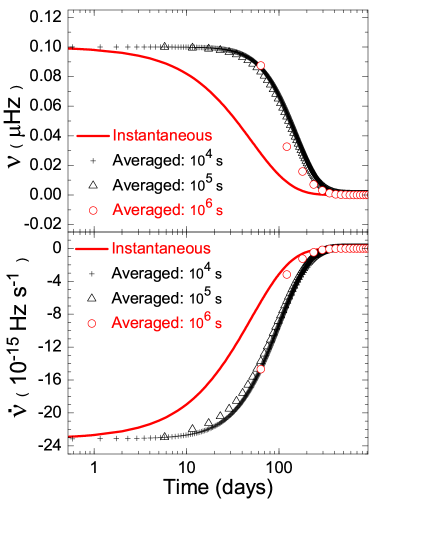
Figure 1: Variations of $\nu$ (upper panel) and $\dot{\nu}$ (bottom panel) for a simulated classical glitch with one decay term. Solid lines represent their instantaneous values; circles, triangles, and crosses represent the averaged values obtained by fitting the simulated TOAs to Equation (1) for the cases of $\Delta T_{\rm int}=10^{4}$, $10^{5}$, and $10^{6}$ s, respectively.

However with the TEMPO2 software, $\nu$ may be obtained from the TOAs by fitting to

$$\Phi_{i}={\Phi}+\nu(t_{i}-t),$$ (7)

and $\dot{\nu}$ may be obtained by fitting to

$$\Phi_{i}={\Phi}+\nu(t_{i}-t)+\frac{1}{2}\dot{\nu}(t_{i}-t)^{2},$$ (8)

i.e. the first two or three terms of Equations (1), respectively (Yu 2013). Here, we first fit the TOA blocks to Equation (7) to obtain $\nu_{\rm A}$, which is the fitted coefficients of $\nu$ term of Equation  (7). We then separately fit the TOA blocks to Equation (8) to obtain $\dot{\nu}_{\rm A}$, which is the fitted coefficients of $\dot{\nu}$ term of Equation  (8). In the left panels of Figure 2, we show the instantaneous and averaged values obtained this way, with different $\Delta T_{\rm int}$ for a glitch with the same $\Delta\nu_{\rm d}$ and $\tau$. Clearly now the profiles of both $\nu_{\rm A}$ and $\dot{\nu}_{\rm A}$ follow that of $\nu_{\rm I}$ and $\dot{\nu}_{\rm I}$ without obvious distortions. By fitting to Equation (2) or Equation (3), we find that all the recovery time scales of $\nu_{\rm A}$ or $\dot{\nu}_{\rm A}$ equal the time scale of $50$ days, i.e. $\tau$ has not been biased.

We can then obtain the normally reported glitch parameters $\Delta\nu_{\rm d}$ and $\Delta\dot{\nu}_{\rm d}$, as listed in Table 1, by fitting $\{\nu_{\rm A}\}$ or $\{\dot{\nu}_{\rm A}\}$ to Equation (2) or Equation (3) with different $\Delta T_{\rm int}$; for comparison we also list $\Delta\nu_{\rm d}$ and $\Delta\dot{\nu}_{\rm d}$ obtained from $\nu_{\rm I}$ and $\dot{\nu}_{\rm I}$. One can see that “averaged” $\Delta\nu_{\rm d}$ or $\Delta\dot{\nu}_{\rm d}$ (denoted as $\Delta\nu_{\rm dA}$ or $\Delta\dot{\nu}_{\rm dA}$ hereafter) have systematic differences from instantaneous $\Delta\nu_{\rm d}$ or $\Delta\dot{\nu}_{\rm d}$ (denoted as $\Delta\nu_{\rm dI}$ or $\Delta\dot{\nu}_{\rm dI}$ hereafter). For $\Delta T_{\rm int}=10^{4}~{}{\rm s}$, the differences are tiny and the glitch parameters can be restored satisfactorily; however, for $\Delta T_{\rm int}\geqslant 10^{5}~{}{\rm s}$, both the “averaged” $\Delta\nu_{\rm d}$ and $\Delta\dot{\nu}_{\rm d}$ may be considerably smaller than the instantaneous $\Delta\nu_{\rm d}$ and $\Delta\dot{\nu}_{\rm d}$, respectively.

For a slow glitch, we assume

$$\nu(t)=\Delta\nu_{\rm d}(1-\exp{(-\Delta t/\tau)}),$$ (9)

where $t_{0}=0$ and $\Delta\nu_{\rm d}=0.1~{}\textmd{$\mu$Hz}$ and $\tau=50~{}\textmd{days}$. We show the averaged glitch parameters and profiles with different $\Delta T_{\rm int}$ in Table 1 and the right panels of Figure 2, as well as those instantaneous ones. One can see that we always have $\Delta\nu_{\rm dA}=\Delta\nu_{\rm dI}$ for any $\Delta T_{\rm int}$, since $\Delta\nu_{\rm dA}$ is determined by the differences of $|\dot{\nu}_{\rm A}|$ between the data points slightly before the starting point of the glitch and the data points at the end of the recovery, and both of them are always available for slow glitch observations. However, $\Delta\dot{\nu}_{\rm dA}$ is biased in the same way as for the simulated classical glitch.

Table 1: $\Delta\nu_{\rm d}$ ($\mu$Hz), $\Delta\dot{\nu}_{\rm d}$ ($10^{-15}$ Hz s^-1) and $\tau$ (days) for classical (upper part) and slow (bottom part) glitch simulations. The data in left part and right part are results from one decay term and two decay term simulations, respectively. “Instantaneous” represents the instantaneous values, and the different values of $\Delta T$ represent the time intervals between each TOA for the “averaged” values.

	$\Delta\nu_{\rm d}$	$\Delta\dot{\nu}_{\rm d}$	$\tau$	$\Delta\nu_{\rm d}$	$\Delta\dot{\nu}_{\rm d}$	$\tau$
Instantaneous	0.100	-23.15	50.00	(0.19, 0.119)	(-102.8, -9.4)	(21.4, 147.0)
$\Delta T_{\rm int}=10^{4}~{}{\rm s}$	0.099	-22.88	50.00	(0.18, 0.119)	(-100.2, -9.4)	(21.3, 145.8)
$\Delta T_{\rm int}=10^{5}~{}{\rm s}$	0.089	-20.67	50.00	(0.13, 0.139)	(-100.4, -16.8)	(14.5, 95.6)
$\Delta T_{\rm int}=10^{6}~{}{\rm s}$	0.041	-9.53	49.52	(2.73, 0.081)	(-2960.9, -6.4)	(10.7, 146.8)
Instantaneous	0.100	23.15	50.00	(0.19, 0.119)	(102.8, 9.4)	(21.4, 147.0)
$\Delta T_{\rm int}=10^{4}~{}{\rm s}$	0.100	23.04	49.95	(0.19, 0.120)	(100.2, 9.4)	(21.3, 145.8)
$\Delta T_{\rm int}=10^{5}~{}{\rm s}$	0.100	20.67	49.99	(0.19, 0.122)	(100.4, 16.8)	(14.5, 95.7)
$\Delta T_{\rm int}=10^{6}~{}{\rm s}$	0.100	9.88	49.36	(0.25, 0.055)	(2959.0, 6.4)	(10.7, 146.8)

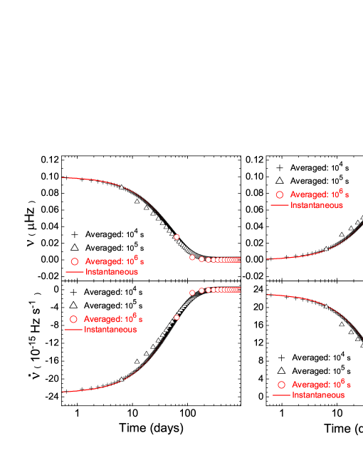
Figure 2: Variations of $\nu$ and $\dot{\nu}$ for a simulated classical glitch (left panels) and a simulated slow glitch (right panels) with one decay term. Solid lines represent their instantaneous values; circles, triangles, and crosses represent the averaged values obtained by fitting the simulated TOAs to Equations (7) (to get $\nu_{\rm A}$) and (8) (to get $\dot{\nu}_{\rm A}$) for the cases of $\Delta T_{\rm int}=10^{4}$, $10^{5}$, and $10^{6}$ s, respectively.

2.1.2 Simulation for Two Decay Terms

We simply assume $\nu(t)=\Delta\nu_{{\rm d}1}\exp{(-t/\tau_{1})}+\Delta\nu_{{\rm d}2}\exp{(-t/\tau_{2})}$ for a classical glitch with two decay terms, where $\Delta\nu_{{\rm d}1}=0.19$ $\mu$Hz, $\tau_{1}=21.4~{}\textmd{days}$ and $\Delta\nu_{{\rm d}2}=0.119$ $\mu$Hz, $\tau_{2}=147~{}\textmd{days}$ (the parameters are adopted from pulsar B2334+61 for its very large glitch between 2005 August 26 and September 8, Yuan et al. 2010). We also assume $\nu(t)=\Delta\nu_{{\rm d}1}(1-\exp{(-t/\tau_{1})})+\Delta\nu_{{\rm d}2}(1-\exp{(-t/\tau_{2})})$ for a slow glitch with two decay terms. The instantaneous values and averaged values are obtained with the same methods described above and the main results are presented in Table 1 and Figure 3, in which the similar results can be found with the case of one decay term. For $\Delta T_{\rm int}=10^{4}~{}{\rm s}$, the differences for all of $\tau$, $\Delta\nu_{\rm d}$ and $\Delta\dot{\nu}_{\rm d}$ are tiny and the glitch parameters can be restored satisfactorily. However, things for two decay terms are a little more complicated. For $\Delta T_{\rm int}\gtrsim 10^{5}~{}{\rm s}$, though the data points still converged to the instantaneous values as shown in Figure 3 (i.e. variation trends are the same), the fitted glitch parameters (including $\tau$) for each components are still somewhat biased, and it seems that larger $\Delta T_{\rm int}$ corresponds to a smaller $\tau$ for short time-scale component. The biases are probably due to the fact that the data are too sparse for $\Delta T_{\rm int}$. Actually if $\tau$ of the short term decay component is comparable to or shorter than the interval between the observations, then $\tau$ of this component would be difficult to determine and can only be set as the internal. Similar results can be found for a slow glitch, but $\sum\Delta\nu_{\rm dI}=\sum\Delta\nu_{\rm dA}$ is always kept.

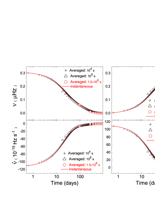
Figure 3: Variations of $\nu$ and $\dot{\nu}$ for a simulated classical glitch (left panels) and a simulated slow glitch (right panels) with two decay terms. Solid lines represent their instantaneous values; circles, triangles, and crosses represent the averaged values obtained by fitting the simulated TOAs to Equations (7) (to get $\nu_{\rm A}$) and (8) (to get $\dot{\nu}_{\rm A}$) for the cases of $\Delta T_{\rm int}=1.5\times 10^{6}$, $10^{5}$, and $10^{4}$ s, respectively.

The above simulations unveil significant biases caused by the averaging procedures (i.e. fitting to Equation (7) and Equation (8)) for $\nu$ and $\dot{\nu}$ during glitch recoveries. Thus, $\nu_{\rm A}$ and $\dot{\nu}_{\rm A}$ obtained this way and $\nu_{\rm O}$ and $\dot{\nu}_{\rm O}$ (the subscript “o” means observed values) reported in literature should not be used directly to test physical models. It should be noted that, for one-decay-term cases, the reported amplitudes of $\Delta{\nu}$ and $\Delta\dot{\nu}$ of a classical glitch are usually underestimated; the reported amplitude of $\Delta\dot{\nu}$ of a slow glitch is also underestimated, but that $\Delta{\nu}$ is not. However, these biases were never noticed in almost all previous theoretical works modeling glitch recoveries, and $\{\dot{\nu}(t)\}$ are usually directly modeled, e.g. the post-glitch fits for Vela pulsar, Crab pulsar and PSR 0525+21 with vortex creep model (Alpar et al. 1984b; Alpar, Nandkumar, & Pines 1985; Alpar et al. 1993; Chau et al. 1993; Alpar, et al. 1996; Larson & Link 2002), and the two-component hydrodynamic model for Vela (van Eysden & Melatos 2010). In these works, the observed data $\{\dot{\nu}_{\rm O}(t)\}$ (i.e. $\{\dot{\nu}_{\rm A}(t)\}$) are shown in $\dot{\nu}$-$t$ diagram and fitted directly by theoretical models.

2.2 Simulation for Phase-fitting procedure

In order to make optimum use of all available data (Shemar & Lyne 1996), the pulse phase induced by a glitch is usually fitted to the following equation, which can give $\tau$ and $\Delta\nu_{d}$ (e.g. Yu et al. 2013):

$$\phi_{\rm g}={\Delta\phi}+\nu_{\rm p}\Delta t+\frac{1}{2}\dot{\nu}_{\rm p}\Delta t^{2}+[1-e^{-(\Delta t/\tau_{i})}]\Delta\nu_{{\rm d}i}\tau_{i},$$ (10)

where the $\nu_{\rm p}$ and $\dot{\nu}_{\rm p}$ are the permanent increments in $\nu$ and $\dot{\nu}$, respectively. However, it is difficult to get $\tau_{i}$ directly by fitting to Equation (10). Actually, TEMPO2 implements only a linear fitting algorithm, and one thus needs to have a good initial estimate for $\tau_{i}$, which is estimated from post-glitch $\dot{\nu}$ variation by eye inspecting. Then the estimated value was introduced into Equation (10) fits. By increasing or decreasing $\tau_{i}$, a best estimated $\tau_{i}$ can be eventually found via minimum post-fit $\chi^{2}$ (Yu et al. 2013). This procedure is widely used for classical glitches, but not applied to slow glitches.

We simulate the fitting procedure of Equation (10) as described above, and find that both $\tau$ and $\Delta\nu_{\rm d}$ can be obtained with high precision for one-decay-term case, if a good initial estimate for $\tau$ is taken, as shown in Table 2. For two-decay-term case, we also assume $\nu(t)=\Delta\nu_{{\rm d}1}\exp{(-t/\tau_{1})}+\Delta\nu_{{\rm d}2}\exp{(-t/\tau_{2})}$, where $\Delta\nu_{{\rm d}1}=0.119$ $\mu$Hz, $\tau_{1}=147~{}\textmd{days}$ and $\Delta\nu_{{\rm d}2}=0.19$ $\mu$Hz, $\tau_{2}=21.4~{}\textmd{days}$, and get the phase by $\Phi(t)=\int\nu(t)dt$. Firstly, we estimate $\tau_{1}$ for the long term one, and get the best-fit $\tau_{1}$ by fitting $\{\Phi(t_{i})\}$ to Equation (10). Then we fix $\tau_{1}$ and get the timescale of the short term $\tau_{2}$ the same way. This process is widely adopted in the data analysis of glitch recovery with TEMPO2 software (Yu et al. 2003). However, we find that the glitch parameters of the long decay term in the two term cases, i.e $\tau_{1}$ and $\Delta\nu_{\rm d1}$ obtained by this way are already biased, as shown in Table 2.

Table 2: $\Delta\nu_{\rm d}$ ($\mu$Hz), $\tau$ (days) for classical glitch simulations with direct phase-fit procedure. The data in left part and right part are the results from one decay term and two decay term simulations, respectively. Subscript “1” indicates the long decay term in two term cases.

	$\Delta\nu_{\rm d}$	$\tau$	$\Delta\nu_{\rm d1}$	$\tau_{1}$
Instantaneous	0.100	50.00	0.119	147.0
$\Delta T_{\rm int}=10^{4}~{}{\rm s}$	0.109	50.00	0.150	128.0
$\Delta T_{\rm int}=10^{5}~{}{\rm s}$	0.108	50.00	0.151	127.6
$\Delta T_{\rm int}=10^{6}~{}{\rm s}$	0.106	50.00	0.158	124.0

These biases are probably caused by the procedure that fitting the long-decay-term and the short-decay-term in different steps; the short-decay-term may slightly interfere the first fitting for $\tau_{1}$ and $\Delta\nu_{{\rm d}1}$ of the long-decay-term, thus the results are biased. If the biased $\tau_{1}$ is fixed, one will also get a biased $\tau_{2}$ to fit $\{\Phi(t_{i})\}$ again to Equation (10), since a local minimum $\chi^{2}$ will obtained, as shown in Figure 4. Therefore, we suggest that the two terms should be fitted simultaneously.

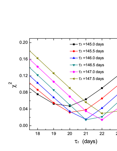
Figure 4: The local minimum of $\chi^{2}$ produced by fitting $\{\Phi(t_{i})\}$ to Equation (10). During each fitting, $\tau_{1}$ is fixed to a certain value around 147 days.

If $\Delta T_{\rm int}\lesssim 10^{4}$ s, the simultaneous fits can be realized by the following steps:

(i) Get $\{\dot{\nu}\}$ series by fitting $\{\Phi(t_{i})\}$ to Equation (8);

(ii) Estimate $\tau_{1}$ and $\tau_{2}$ by fitting $\{\dot{\nu}\}$ to Equation (3) (the calculation cost needed by this fit is much lower than fitting to Equation (10));

(iii) Use the estimated $\tau_{1}$ and $\tau_{2}$ as initial values and fit $\{\Phi(t_{i})\}$ again to Equation (10), then the best fitted $\tau_{i}$ and $\Delta\nu_{{\rm d}i}$ will be obtained.

The results of the simultaneous fit are $\Delta\nu_{{\rm d}1}=0.119$ $\mu$Hz, $\tau_{1}=147.0~{}\textmd{days}$ and $\Delta\nu_{{\rm d}2}=0.190$ $\mu$Hz, $\tau_{2}=21.4~{}\textmd{days}$, which are exactly the same with those introduced in the model; the results are independent with $\Delta T_{\rm int}$. We also simulate the fitting processes with different values of $\tau_{i}$ and $\Delta\nu_{{\rm d}i}$, and all the glitch parameters are restored with relatively small biases, some of which are even better than the previous procedures for $\Delta T_{\rm int}\lesssim 10^{4}$ s. Here, we want emphasize that the fitting procedures described in literature are in chaos. Many authors adopted the procedure of fitting the TOAs to Equation (10) to obtain the pulsars parameters, and using Equation (8) to get $\{\dot{\nu}\}$, but only Equation (1) is mentioned in their papers (Yu 2013). Thus, we suggest that the exact fitting procedure should be described in detail.

3 A Phenomenological Spin-down Model

In this section, we develop a phenomenological spin-down model to describe the glitch and slow glitch recoveries, so that the model can be a tool to simulate data to test the data analysis procedures for the recoveries in the next section. Classically, a magnetic dipole with a magnetic moment $M=BR^{3}$, rotating in vacuum with angular velocity $\Omega$, emits electromagnetic radiation with a total power $2M^{2}\Omega^{4}/3c^{3}$. Assuming the pure magnetic dipole radiation as the braking mechanism for a pulsar’s spin-down, the energy loss rate is then given by

$$\dot{E}=I\Omega\dot{\Omega}=-\frac{2(BR^{3}\sin\chi)^{2}}{3c^{3}}{\Omega^{4}},$$ (11)

where $B$ is its dipole magnetic field at its magnetic pole, $R$ is its radius, $I$ is its moment of inertia. Equation (11) is modified slightly in order to describe a glitch event,

$$\dot{\Omega}\Omega^{-3}=-\frac{2(BR^{3}\sin\chi)^{2}}{3c^{3}I}G(t),$$ (12)

in which $G(t)$ represents very small changes in the effective strength of dipole magnetic field $B\sin\chi$, or the effective moment of inertia $I$ of both the pulsar and its magnetosphere during a glitch recovery. The left hand are observable quantities, and the right hand are all theoretical quantities. In the following we assume $G(t)=1+\kappa e^{-\Delta t/\tau}$. Then Equation (12) can be written as

$$\dot{\nu}\nu^{-3}=-H_{0}(1+\kappa e^{-\Delta t/\tau}),$$ (13)

where $\dot{\nu}=\dot{\Omega}/2\pi$ and $H_{0}=\frac{8\pi^{2}(BR^{3}\sin\chi)^{2}}{3c^{3}I}=1/2\tau_{\rm c}\nu_{0}^{2}$, and $\tau_{\rm c}=-\nu/2\dot{\nu}$ is the characteristic age of a pulsar.

Integrating and solving Equation (13), we have

$$\nu(t)=\frac{\nu_{0}}{\sqrt{1+(\Delta t+\kappa\tau(1-e^{-(\Delta t)/\tau}))/\tau_{\rm c}}}.$$ (14)

The derivative of $\nu$ is

$$\dot{\nu}(t)=-\frac{(1+\kappa e^{-\Delta t/\tau})\nu_{0}/2\tau_{\rm c}}{(1+(\Delta t+\kappa\tau(1-e^{-\Delta t/\tau}))/\tau_{\rm c})^{3/2}}.$$ (15)

We know $\Delta t\sim\tau\sim 100~{}{\rm days}$ and generally $\tau_{\rm c}\gtrsim 10^{4}~{}{\rm years}$, and the term $|(\Delta t+\kappa\tau(1-e^{-\Delta t/\tau}))/\tau_{\rm c}|\ll 1$ and $\kappa\ll 1$, the expression of $\nu$ and $\dot{\nu}$ can be approximately written in the same forms of Equations (2) and (3), which give $\Delta\nu_{{\rm d}}=\nu_{0}\kappa\tau/2\tau_{\rm c}$ and $\Delta\dot{\nu}_{{\rm d}}=-\nu_{0}\kappa/2\tau_{\rm c}$. Numerical calculations show that Equations (2) and (3) with these parameters give identical results as Equations (14) and (15) for all known ranges of glitch parameters. The expression of $\Delta\nu_{\rm p}$ and $\Delta\dot{\nu}_{\rm p}$ that relate to the initial jumps of $\nu_{0}$ and $\dot{\nu}_{0}$, are not given by the model, since the glitch relaxation processes are only considered here. It has been suggested that these non-recoverable jumps are the consequence of permanent dipole magnetic field increase during the glitch event (Lin and Zhang 2004). $\Delta\ddot{\nu}_{\rm p}$ is the jump of timing residual, which is beyond the scope of the present work.

In the following we attempt to apply this phenomenological model to fit the reported data of several slow glitches of B1822–09 and one classical glitch of B2334+61. Since the reported data points of $\nu$ and $\dot{\nu}$ are too sparse (about one point per 150 days for B1822–09 or 50 days for B2334+61) and the TOAs of these glitches are not available in literature, we cannot apply our model to fit the reported to obtain both $\tau$ and $\kappa$ simultaneously, as that done in the above simulations. As a compromise, we focus only on determining $\kappa$ by applying our phenomenological model and simply take (the inevitably biased) $\tau$ obtained by fitting directly the reported $\nu$ and $\dot{\nu}$. Therefore $\kappa$ remains the only glitch recovery parameter to be determined from observations in the following. Our main purpose here is to show the applicability of the our phenomenological model to describe glitch observations.

3.1 Modeling several slow glitches of B1822–09

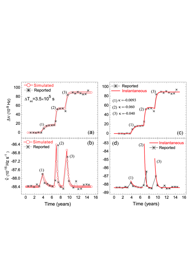
Figure 5: Slow glitches of Pulsar B1822–09. Observational results are taken from Shabanova (2005). Upper panels: variations of $\Delta\nu$ relative to the pre-glitch solution. Bottom panels: variations of $\dot{\nu}$. Left panels: comparison between the reported and simulated (both are also time-averaged) $\Delta\nu$ and $\dot{\nu}$. Right panels: comparison between the reported and restored (i.e. model-predicted) instantaneous $\Delta\nu$ and $\dot{\nu}$.

We first model slow glitches because they are simpler than the classical glitches, especially they have no jumps in $\nu$ and $\dot{\nu}$, i.e. $\Delta\nu_{\rm p}=0$ and $\Delta\dot{\nu}_{\rm p}=0$. Shabanova (2005) reported three slow glitches of B1822–09 (J1825-0935) over the 1995-2004 interval. The pulsar has $\nu\simeq 1.30~{}{\rm s}^{-1}$, a relatively large $|\dot{\nu}|\simeq 8.878\times 10^{-14}~{}{\rm s}^{-2}$ (note $\dot{\nu}<0$), implying $\tau_{\rm c}\simeq 232$ kyr and $B\simeq 6.43\times 10^{12}$ G. As shown in Figure 5, the pulsar experienced three slow glitches from 1995 to 2005. A gradual increase in $\nu$ is well modeled by an exponential function with timescales of $235$, $80$ and $110$ days, respectively. For $\dot{\nu}$, the fractional decreases of $|\dot{\nu}|$ (i.e. increases of $\dot{\nu}$) are about $0.7$, $2.7$ and $1.7$ percent, respectively. The subsequent increases of $|\dot{\nu}|$ (i.e. decreases of $\dot{\nu}$) back to the previous values with the same time scales are also well described by exponential functions. The third slow glitch was separately detected by Zou et al. (2004).

Since the detailed data on $\Delta T_{\rm int}$ are not reported in literature, we assume an uniform TOA distribution with $\Delta T_{\rm int}=3.5\times 10^{5}$ s. We take the following steps in modeling the observed data for each slow glitch event:

(i) We get our model-predicted TOAs with $\Delta T_{\rm int}$ by integrating Equations (2) or (14), with a $\kappa$ for each slow glitch event.

(ii) We simulate the data analysis process by fitting every block of ten adjacent TOAs to Equations (7) or Equations (8) to obtain one set of $\nu_{\rm A}$ and $\dot{\nu}_{\rm A}$; and the latter five TOAs are also used in the next TOA block.

(iii) The above simulated $\nu_{\rm A}$ and $\dot{\nu}_{\rm A}$ are compared with the reported glitch profile $\nu_{\rm O}$ and $\dot{\nu}_{\rm O}$; $\kappa$ is adjusted until reasonable agreements between them are reached.

With the above steps, we confirm that the slow glitch behavior can be explained by our phenomenological model with $\kappa<0$. Our modeling results are shown in Figure 5. The fit parameter $\kappa$ is $-0.0093$, $-0.06$ and $-0.04$ for the three slow glitch events, respectively. In Table 3 we show the relative magnitudes of $\Delta\nu$ and $\Delta\dot{\nu}$ for the three slow glitches; for comparison we also list in Table 3 the results for the giant classical glitch from B2334+61 obtained in the next section. It is found that the relative magnitudes of $\Delta\nu_{\rm A}$, $\Delta\nu_{\rm O}$ and $\Delta\nu_{\rm I}$ are identical, i.e. $\Delta\nu_{\rm I}=\Delta\nu_{\rm A}=\Delta\nu_{\rm O}$, as expected from the above simulations. It is also clear that the instantaneous values of $\Delta\dot{\nu}$, which are calculated directly from the model with the parameters determined above, are much larger than the reported results in literature, e.g. the $\Delta\dot{\nu}_{\rm I}$ are larger than two times of $\Delta\dot{\nu}_{\rm O}$ for the second and third slow glitches.

Table 3: The relative values of $\Delta\nu$ and $\Delta\dot{\nu}$ for slow glitches of B1822–09 and the giant classical glitch from B2334+61. In the classical glitch part, the superscripts ‘${\rm i}$’ and ‘${\rm ii}$’ represent for results of one-term fit and two-term fit, respectively.

	Slow Glitches of B1822–09						Classical Glitch of B2334+61
	$\Delta\nu_{1}/\nu_{0}$	$\Delta\dot{\nu}_{1}/\dot{\nu}_{0}$	$\Delta\nu_{2}/\nu_{0}$	$\Delta\dot{\nu}_{2}/\dot{\nu}_{0}$	$\Delta\nu_{3}/\nu_{0}$	$\Delta\dot{\nu}_{3}/\dot{\nu}_{0}$	$\Delta\nu^{\rm i}/\nu_{0}$	$\Delta\dot{\nu}^{\rm i}/\dot{\nu}_{0}$	$\Delta\nu^{\rm ii}/\nu_{0}$	$\Delta\dot{\nu}^{\rm ii}/\dot{\nu}_{0}$
	($10^{-9}$)	(%)	($10^{-9}$)	(%)	($10^{-9}$)	(%)	($10^{-9}$)	(%)	($10^{-9}$)	(%)
Reported	12.9	0.7	28.6	2.7	25.2	1.7	75.8	-2.96	75.8	-2.96
Simulated	13.2	0.7	29.7	2.7	25.4	2.0	35.6	-3.15	54.5	-2.87
Instantaneous	13.2	0.94	29.7	6.0	25.4	4.0	64.4	-3.85	79.8	-3.98

3.2 Modeling one classical glitch of B2334+61

The pulsar PSR B2334+61 (PSR J2337+6151) was discovered in the Princeton-NRAO survey using the 92 m radio telescope at Green Bank in 1985 (Dewey et al. 1985). It has $\nu\simeq 2.019~{}{\rm s^{-1}}$, $\dot{\nu}\simeq-788.332\times 10^{-15}~{}{\rm s^{-2}}$, $\tau_{\rm c}\simeq 4.1\times 10^{4}~{}{\rm yr}$, and $B\simeq 9.91\times 10^{12}$ G. It is located very close to the center of the supernova remnant G114.3+0.3. Yuan et al. (2010) reported the timing observations of PSR B2334+61 for seven years with the Nanshan 25 m telescope at Urumqi Observatory. A very large glitch occurred between 2005 August 26 and September 8 (MJDs 53608 and 53621), the largest known glitch ever observed, with a fractional frequency increase of $\Delta\nu/\nu\sim 20.5\times 10^{-6}$. Yuan et al. (2010) obtained each $\nu$, $\dot{\nu}$ and $\ddot{\nu}$ by fitting ten adjacent TOAs to Equation (1), and the latter five TOAs had also been used as the first five TOAs in the next fit. The rotational behavior during this glitch event is shown in Figure 6. A large jump of rotational frequency could be seen in the top panel with $\Delta\nu\approx 41\times 10^{-6}$ Hz. The bottom panel shows a very significant long-term increase in $|\dot{\nu}|$ after the time of jump, and the corresponding braking indices are $10.5\pm 0.2$ and $46.8\pm 0.3$ before and after the glitch, respectively. The recovery process following the glitch was described by a dominant rapid exponential decay with a time scale of $\sim 21.4$ days and an additional slower decay with a time scale of $\sim 147$ days (Yuan et al. 2010).

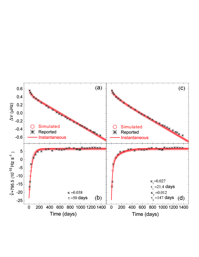
Figure 6: The giant glitch of Pulsar B2334+61. Observational results are taken from Yuan et al. 2010. $\Delta T_{\rm int}=1.8\times 10^{5}~{}{\rm s}$ is adopted in the fit. Upper panels: variations of $\Delta\nu$. Bottom panels: variations of $\dot{\nu}$. The left and right panels represent for models with one and two decay components, respectively.

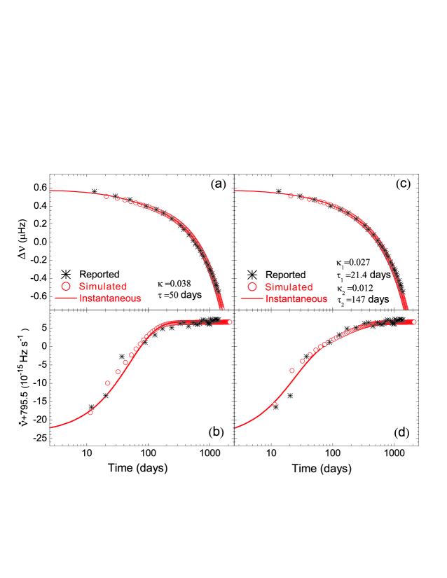
Figure 7: The giant glitch of Pulsar B2334+61. Observational results are taken from Yuan et al. 2010. $\Delta T_{\rm int}=1.8\times 10^{5}~{}{\rm s}$ is adopted in the fit. Upper panels: variations of $\Delta\nu$. Bottom panels: variations of $\dot{\nu}$. The left and right panels represent for models with one and two decay components, respectively. This figure is the same with Fig. 6 except for a logarithmic abscissa.

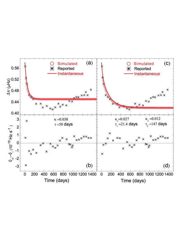
Figure 8: The giant glitch of Pulsar B2334+61. Upper panels: variations of $\Delta\nu$ from which the slope $\Delta\dot{\nu}_{\rm p}$ is removed. Bottom panels: residuals of $\dot{\nu}_{\rm O}-\dot{\nu}_{\rm I}$. The left and right panels represent for models with one and two decay components, respectively.

We follow almost the same steps as for the slow glitches above to model the reported, yet time-averaged glitch recovery data of this classical glitch, with $\Delta T_{\rm int}=1.8\times 10^{5}$ s; the only difference is that a slope of $\Delta\dot{\nu}_{\rm p}=-8.684\times 10^{-15}~{}{\rm s}^{-2}$ is taken in Equation (2), following Lyne et al. (2000).

In the left panels of Figure 6, we show the fits with one exponential term $G(t)=(1+\kappa\exp{(-\Delta t/\tau)})$ for a comparison with the “realistic” simulation of two terms below. The best parameters for this glitch event are $\kappa_{1}=0.038$ and $\tau=50$ days. We then model the glitch recovery process with $G(t)=(1+\kappa_{1}\exp{(-\Delta t/\tau_{1})}+\kappa_{2}\exp{(-\Delta t/\tau_{2})})$, as shown in the right panels of Figure 6. The best parameters for this glitch event are $\kappa_{1}=0.027$ and $\kappa_{2}=0.012$ ($\tau_{1}=21.4$ days and $\tau_{2}=147$ days are fixed by the observed values). Table 3 gives the relative magnitudes of $\Delta\nu$ and $\Delta\dot{\nu}$ for both fits. In order to distinguish between the two fits, we show them in the logarithmic coordinates in Figure 7. Clearly the simulated profiles of the two term fit match the reported ones better than that of the one term fit. One can see that $|\Delta\dot{\nu}_{\rm I}|$ are also slightly larger than the reported $|\Delta\dot{\nu}_{\rm O}|$ for both the one-term fit and two-term fit.

In Figure 8 we show $\Delta\nu$ with the slope of $\Delta\dot{\nu}_{\rm p}$ removed, and $\dot{\nu}_{\rm O}-\dot{\nu}_{\rm I}$. It is clearly shown that one exponential term cannot fit the observed data at the end of decay profile, and this is also the reason why $\Delta\nu_{\rm I}$ is smaller than $\Delta\nu_{\rm O}$ for this fit, as given in Table 3. Thus, the one-term decay is ruled out, and we focus on the two-term fit below. Using $\nu_{0}$, $\tau_{c}$ and the determined $\kappa_{1}$ and $\kappa_{2}$, we obtain these glitch parameters: $\Delta\nu_{\rm d1}=0.039~{}{\rm\mu Hz}$, $\Delta\nu_{\rm d2}=0.119~{}{\rm\mu Hz}$, $\Delta\dot{\nu}_{\rm d1}=-2.1\times 10^{-14}~{}{\rm s}^{-2}$, $\Delta\dot{\nu}_{\rm d2}=-9.38\times 10^{-15}~{}{\rm s}^{-2}$; some of them have significant differences from the reported results of Yuan et al. (2010), in which $\Delta\nu_{\rm d1}=0.19~{}{\rm\mu Hz}$, $\Delta\nu_{\rm d2}=0.119~{}{\rm\mu Hz}$, $\Delta\dot{\nu}_{\rm d1}=-1.03\times 10^{-13}~{}{\rm s}^{-2}$, $\Delta\dot{\nu}_{\rm d2}=-9.37\times 10^{-15}~{}{\rm s}^{-2}$.

In Figure 8, one can also see an exponential increase of $\nu$ after the glitch recovery, which is a very common, but not well understood behavior (Lyne 1992, see an example of a Crab glitch). We suggest that the exponential increase component is probably a slow glitch, and the fact that a slow glitch following a classical glitch recovery may be an important clue to the enigmas of glitch phenomena.

4 Testing Several Fitting Procedures Based on the Phenomenological Spin-down Model

In section 3, we showed that the recovery processes of glitches and slow glitches can be well modeled by the phenomenological model, which can also be used to simulate a real glitch recoveries, in order to fully test different fitting procedures. We get $\Phi(t)$ by integrating Equation (13) for a certain $\tau_{i}$ and $\kappa_{i}$, and get the TOA set $\{\Phi(t_{i})\}$ by assuming a certain $\Delta T_{\rm int}$. We test the biases produced by the following four fitting procedures in the section; three of them are discussed in section 2 for the simplified model of classical and slow glitches. Here all four procedures are examined with a more “realistic” model, i.e., our phenomenological spin-down model.

Fitting Procedure I: obtain $\{\dot{\nu}(t_{i})\}$ by fitting $\{\Phi(t_{i})\}$ to Equation (1), and get $\tau$ and $\Delta\nu_{\rm d}$ by fitting $\{\dot{\nu}(t_{i})\}$ to Equation (3) (e.g. Roy et al. 2012, Espinoza et al. 2011, Yuan et al. 2010, Zou et al. 2008, Zou et al. 2004, Dall’Osso et al. 2003, Urama 2002, Dodson et al. 2002, McCulloch et al. 1990). We take $\tau=50$ days, $\kappa=0.03$ in the model, and show instantaneous results and the fitted results for different $\Delta T_{\rm int}$ in Table 4. The instantaneous $\Delta\nu_{\rm d}$ is given by $\Delta\nu_{{\rm d}}=\nu_{0}\kappa\tau/2\tau_{\rm c}$. It is found that both $\tau$ and $\Delta\nu_{\rm d}$ are seriously biased. It is also noticed that the total time span $T_{\rm s}$ (i.e. the time span from the begin of the glitch to the end of the recovery assumed), has considerable impact on the fitting results else. We take higher order polynomials to fit the phase and find that $\tau$ is also seriously biased, even worse than the lower order one. Thus, if one takes a higher order polynomial and calls the first (linear) term “frequency” then this is clearly not a good approximation, since a higher order polynomial would lead to this not being the “frequency”, given that part of it is reabsorbed into other coefficients.

Table 4: Classical glitch simulations with the phenomenological model. $\Delta\nu_{\rm d}$ (0.1 $\mu$Hz) and $\tau$ (days) obtained by fitting procedure I.

	$T_{\rm s}=1~{}{\rm year}$		$T_{\rm s}=3~{}{\rm years}$		$T_{\rm s}=5~{}{\rm years}$
	$\tau$	$\Delta\nu_{\rm d}$	$\tau$	$\Delta\nu_{\rm d}$	$\tau$	$\Delta\nu_{\rm d}$
Instantaneous	50	1.01	50	1.01	50	1.01
$\Delta T_{\rm int}=10^{4}~{}{\rm s}$	213.38	1.15	96.45	2.35	92.34	2.22
$\Delta T_{\rm int}=10^{5}~{}{\rm s}$	161.99	6.49	90.74	2.51	87.52	2.11
$\Delta T_{\rm int}=10^{6}~{}{\rm s}$	27.02	3.68	37.75	3.07	38.75	3.04

Fitting Procedure II: obtain $\{\dot{\nu}(t_{i})\}$ by fitting $\{\Phi(t_{i})\}$ to Equation (8), and get $\tau$ and $\Delta\nu_{\rm d}$ by fitting $\{\dot{\nu}(t_{i})\}$ to Equation (3) (e.g. Shabanova 2005, Shabanova 1998). Firstly, we conduct the one decay component case and take $\tau=50$ days, $\kappa=0.03$ in the model. The main results are shown in Table 5. One can see that the instantaneous values can be well restored for $\Delta T_{\rm int}=10^{4}~{}{\rm s}$, and the results with $\Delta T_{\rm int}=10^{5}~{}{\rm s}$ are also good approximations. Then, we conduct the two-component case and take $\tau_{1}=21.7$ days, $\tau_{2}=147$ days, and $\kappa_{1}=0.131$, $\kappa_{2}=0.012$ in the model. One can see that the instantaneous values can only be restored for $\Delta T_{\rm int}=10^{4}~{}{\rm s}$. It is noticed that $T_{\rm s}$ should be long enough for both the one-component and two-component cases. Thus, this procedure is a good approximation on very small $\Delta T_{\rm int}$.

Table 5: Classical glitch simulations with the phenomenological model. $\Delta\nu_{\rm d}$ (0.1 $\mu$Hz) and $\tau$ (days) obtained by fitting procedure II.

	$T_{\rm s}=1~{}{\rm year}$		$T_{\rm s}=3~{}{\rm years}$		$T_{\rm s}=5~{}{\rm years}$
	$\tau$	$\Delta\nu_{\rm d}$	$\tau$	$\Delta\nu_{\rm d}$	$\tau$	$\Delta\nu_{\rm d}$
Instantaneous	50	1.01	50	1.01	50	1.01
$\Delta T_{\rm int}=10^{4}~{}{\rm s}$	49.95	1.00	49.97	1.00	49.98	1.00
$\Delta T_{\rm int}=10^{5}~{}{\rm s}$	45.84	0.95	47.82	0.96	48.01	0.96
$\Delta T_{\rm int}=10^{6}~{}{\rm s}$	22.23	5.02	27.37	3.15	27.85	2.42
Instantaneous	(21.40, 147.00)	(1.90, 1.19)	(21.40, 147.00)	(1.90, 1.19)	(21.40, 147.00)	(1.90, 1.19)
$\Delta T_{\rm int}=10^{4}~{}{\rm s}$	(21.14, 113.58)	(1.85, 0.86)	(21.26, 144.47)	(1.87, 1.18)	(21.27, 145.45)	(2.33, 1.20)
$\Delta T_{\rm int}=10^{5}~{}{\rm s}$	(2.26, 23.86)	(0.59, 1.70)	(9.58, 42.54)	(0.76, 1.57)	(14.40, 81.41)	(1.90, 1.45)

Fitting Procedure III: get $\tau$ and $\Delta\nu_{\rm d}$ directly by fitting $\{\Phi(t_{i})\}$ to Equation (10) (Yu et al. 2013, Edwards et al. 2006, Shemar & Lyne 1996). Firstly, we also conduct the one decay component case and take $\tau=50$ days, $\kappa=0.03$ in the model. The main results are shown in upper part of Table 6. It is found that the instantaneous values can be well restored and the fit results is nearly independent of $\Delta\ T_{\rm int}$. Then, we conduct the two-component case and take $\tau_{1}=21.7$ days, $\tau_{2}=147$ days, and $\kappa_{1}=0.131$, $\kappa_{2}=0.012$ in the model. We fit the two decay terms simultaneously (at a high computing cost) and the main results are shown in the bottom part of Table 6. It is also found that the instantaneous values can be restored satisfactorily and the results are independent of $\Delta\ T_{\rm int}$. However, $T_{\rm s}$ should not be too long for both the one component and two components cases, which is opposite to procedure II.

Table 6: Classical glitch simulations with the phenomenological model. $\Delta\nu_{\rm d}$ (0.1 $\mu$Hz) and $\tau$ (days) obtained by fitting procedure III.

	$T_{\rm s}=1~{}{\rm year}$		$T_{\rm s}=3~{}{\rm years}$		$T_{\rm s}=5~{}{\rm years}$
	$\tau$	$\Delta\nu_{\rm d}$	$\tau$	$\Delta\nu_{\rm d}$	$\tau$	$\Delta\nu_{\rm d}$
Instantaneous	50.00	1.01	50	1.01	50	1.01
$\Delta T_{\rm int}=10^{4}~{}{\rm s}$	50.16	1.02	53.13	0.99	67.23	0.83
$\Delta T_{\rm int}=10^{5}~{}{\rm s}$	50.16	1.02	53.11	0.99	67.01	0.84
$\Delta T_{\rm int}=10^{6}~{}{\rm s}$	50.15	1.02	52.86	1.00	65.29	0.87
Instantaneous	(21.40, 147.00)	(1.90, 1.19)	(21.40, 147.00)	(1.90, 1.19)	(21.40, 147.00)	(1.90, 1.19)
$\Delta T_{\rm int}=10^{4}~{}{\rm s}$	(21.38, 147.92)	(1.92, 1.20)	(21.73, 152.13)	(1.92, 1.20)	(18.98, 160.90)	(2.33, 1.20)
$\Delta T_{\rm int}=10^{5}~{}{\rm s}$	(21.40, 147.93)	(1.92, 1.20)	(21.76, 152.17)	(1.92, 1.20)	(19.04, 160.87)	(2.31, 1.20)
$\Delta T_{\rm int}=10^{6}~{}{\rm s}$	(21.40, 147.96)	(1.92, 1.20)	(21.77, 152.19)	(1.93, 1.20)	(19.35, 160.57)	(2.20, 1.20)

Fitting Procedure IV: the phase $\{\Phi(t_{i})\}$ is fitted by a very high order polynomial, such as

$$\Phi(t)={\Phi_{0}}+\nu(t-t_{i})+\frac{1}{2}\dot{\nu}(t-t_{i})^{2}+\frac{1}{6}\ddot{\nu}(t-t_{i})^{3}+\cdots+\frac{1}{50!}\nu^{(50)}(t-t_{i})^{50}.$$ (16)

The fitted polynomial ($\Phi(t)$, a continuous function) can very precisely describe the TOA series $\{\Phi(t_{i})\}$. One can then take its first or second derivative to obtain $\nu$ or $\dot{\nu}$, i.e. $\nu=\Phi^{\prime}(t)$ or $\dot{\nu}=\Phi^{\prime\prime}(t)$. This procedure is suggested by the anonymous referee.

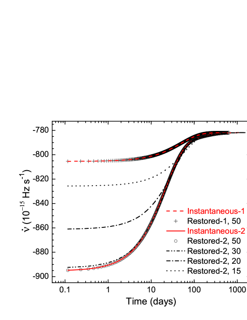
Figure 9: Classical glitch simulations with the phenomenological model. $\dot{\nu}(t)$ for both one and two component cases (denoted as 1 and 2 in the legend, respectively) are obtained by fitting procedure IV. Note that restored results are also continuous functions; here we take their discrete values in order to compare them more conveniently with the instantaneous values. The numbers 50, 30, 20 and 15 in the legend denote the orders of the fitting polynomials.

We also simulate the one component and two component cases, respectively. The results are shown in Figure 9. One can see that the instantaneous values of $\nu(t)$ or $\dot{\nu}(t)$ can be restored with very high precision for both the cases. In the figure, $\Delta T_{\rm int}=10^{6}~{}{\rm s}$ is taken, and it is checked that the results are almost independent of both $\Delta T_{\rm int}$ and $T_{\rm s}$. Then, one can get $\tau_{i}$ and $\Delta\nu_{{\rm d}i}$ by fitting the restored $\dot{\nu}(t)$ to Equation (3). The fitted glitch parameters for one component case are $\tau=50.00$ days and $\Delta\nu_{\rm d}=1.01\times 10^{-7}~{}{\rm Hz}$, and for two component case are $\tau_{1}=21.37$ days, $\tau_{2}=146.93$ days, and $\Delta\nu_{\rm d1}=1.92\times 10^{-7}~{}{\rm Hz}$, $\Delta\nu_{\rm d2}=1.19\times 10^{-7}~{}{\rm Hz}$. They are all consistent with instantaneous values (see e.g. Table 6) with very high precisions. In Figure 9, we show the fitting results of two component case with different order polynomials else. It is found that the order of the polynomial must be very high, e.g. $\gtrsim 35$, which requires that the TOA data points should not be too sparse. We also test the fit procedure with different values of $\tau_{i}$ and $\Delta\nu_{{\rm d}i}$, and all the glitch parameters are restored satisfactorily.

In conclusion, procedure III is a reasonable choice to get $\tau$ and $\Delta\nu_{\rm d}$; however, the two components should be fit simultaneously (in order to avoid some local minimum of $\chi^{2}$), and $T_{\rm s}$ should not be too long. Procedure IV seems to be the best choice for pulsar glitch data analysis, which gives $\{\nu(t)\}$ and $\{\dot{\nu}(t)\}$ with very high precision, and then the glitch parameters $\tau_{i}$ and $\Delta\nu_{{\rm d}i}$ can be satisfactorily estimated by fitting the restored $\dot{\nu}(t)$ to Equation (3). We thus suggest that theorists should always use the full timing solution, rather than try to compare models to individual parameters of fits, as these may be highly inaccurate. Furthermore working in phase seems to be the most accurate and reliable method.

5 Discussions

5.1 How to obtain the correct model parameters of pulsars?

We have shown recently that fitting the observed TOAs of a pulsar to Equation (1) will result in biased (i.e., averaged) spin-down parameters, if its spin-down is non-secular and the variation time scale is comparable to or shorter than the time span of the fitting (Zhang & Xie 2012a, 2012b). In particular we predicted that the reported braking index should be a function of time span and approaches to a small and positive value when the time span is much longer than the oscillation period of its spin-down process, which can be tested with the existing data (Zhang & Xie 2012b).

We notice that in some of the literature (e.g. Roy et al. 2012, Espinoza et al. 2011, Yuan et al. 2010) only Equation (1) is referred to, when describing the fitting process, even for the glitch data analysis. However we have shown in Figure 1 that this will produce a significantly distorted glitch profile. Instead, one can fit to Equations (7) and (8) to obtain the un-distorted (but still averaged) glitch profile; probably this is usually done in practice, though not explicitly described in the literature (Yu 2003). We suggest that the exact fitting procedures should be described when reporting the analysis results of the observed glitch data.

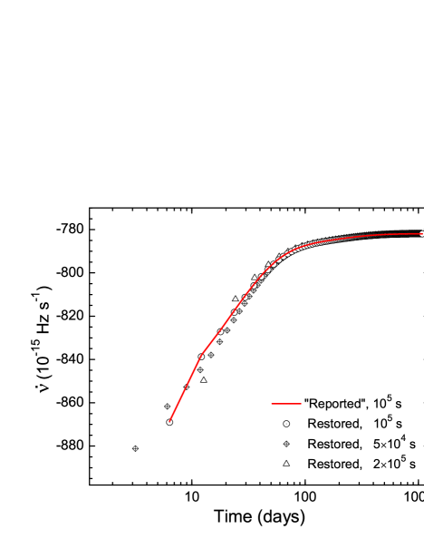
Figure 10: The effects of $\Delta T_{\rm int}$ on variation of $\dot{\nu}$. The “reported” $\{\dot{\nu}\}$ is represented by the solid line, the restored $\{\dot{\nu}\}$ with $\Delta T_{\rm int}=10^{5}$, $5\times 10^{4}$ and $2\times 10^{5}$ s are represented by circles, diamonds and triangles, respectively.

However, neither Equation (1) nor Equations (7) and (8) describe exactly the physical spin-down processes of all pulsars. The pulsar parameters fitted by Equations (10) are also slightly biased especially if $T_{\rm s}$ is not properly taken. Ideally, a spin-down model (empirical, phenomenological or physical) should be used to the fit the observed TOA data, in order to obtain the model parameters. To serve this purpose, the observed TOAs of each pulsar should be made available, and the exact fitting procedure should be described along with the reported spin-down parameters of a pulsar. As shown in Figure 10, we simulate a glitch recovery with parameters $\tau_{1}=21.4$ days, $\tau_{2}=147$ days, and $\Delta\nu_{\rm d1}=1.90\times 10^{-7}~{}{\rm Hz}$, $\Delta\nu_{\rm d2}=1.19\times 10^{-7}~{}{\rm Hz}$, and $\Delta T_{\rm int}=10^{5}$ s. Then we have TOAs from the phenomenological model, and the simulated “reported” $\{\dot{\nu}\}$ is obtained by fitting TOAs to Equation (8) and is represented by the solid line. By fitting TOAs to Equation (10), we have the “reported” glitch parameters $\tau_{1}=21.8$ days, $\tau_{2}=152$ days. With the timescales, we simulate $\{\dot{\nu}\}$ again with $\Delta T_{\rm int}=10^{5}$. The model parameters $\Delta\nu_{\rm d1}$ and $\Delta\nu_{\rm d2}$ can be adjusted until simulated fits match the “reported” ones, and the best fit model parameters $\Delta\nu_{\rm d1}=1.92\times 10^{-7}~{}{\rm Hz}$, $\Delta\nu_{\rm d2}=1.20\times 10^{-7}~{}{\rm Hz}$, which are agree well with original parameters. We show the restored $\{\dot{\nu}\}$ with circles. With the same parameters, the restored $\{\dot{\nu}\}$ for $\Delta T_{\rm int}=5\times 10^{4}$ and $2\times 10^{5}$ s are represented by diamonds and triangles, respectively. One can see that $\{\dot{\nu}\}$ can be well restored if TOAs are known. If $\Delta T_{\rm int}$ taken in simulation is not the right one, the $\{\dot{\nu}\}$ profiles are apparently different from the “reported” one, even though the model parameters are all correct.

When TOAs are available, one can then follow the steps we used above to combine a model with simulations to obtain model parameters. Alternatively, $\Phi(t)$, $\nu(t)$ and $\dot{\nu}(t)$ given by procedure IV can also be fitted directly by physical models.

5.2 The effects of discontinuous observations

In the above analysis, we have assumed that $t_{0}$ is known; however, $t_{0}$ is usually taken as the averaged time of the last reported TOA just before the glitch and the first reported TOA of the glitch. This means we have an uncertainty in $t_{0}$: $\sigma_{t_{0}}=\Delta T_{\rm int}/2$. Then from Equation (6) for a classical glitch, we find

$$\frac{\sigma_{\Delta\nu}}{\Delta\nu}=\frac{\sigma_{\Delta\dot{\nu}}}{\Delta\dot{\nu}}=\frac{\sigma_{t_{0}}}{\tau},$$ (17)

where $\sigma_{\Delta\nu}$ and $\sigma_{\Delta\dot{\nu}}$ are the uncertainties of the restored $\Delta\nu$ and $\Delta\dot{\nu}$, respectively. For the classical glitch of B2334+61, $\sigma_{t_{0}}\sim 4.2$ d, $\tau\sim 21.4$ d. Thus from Equation (17), we have $\sigma_{\Delta\nu}/\Delta\nu=\sigma_{\Delta\dot{\nu}}/\Delta\dot{\nu}\sim 20\%$.

In principle, we have $\sigma_{\Delta\nu}\approx 0$ for a slow glitch, since $\Delta\nu_{\rm d}$ is determined by the data at the end of the recovery, i.e. $\nu\sim\Delta\nu_{\rm d}$ for $\Delta t\gg\tau$ from Equation (9). However, from the derivative of Equation (9), we have $\dot{\nu}=\frac{\Delta\nu_{\rm d}}{\tau}e^{-(t-t_{0})/\tau}$ and $\Delta\dot{\nu}_{\rm d}(\equiv\Delta\nu_{\rm d}/\tau)$ is closely related to $t_{0}$, which resembles the case of a classical glitch. However, for the slow glitch we can fit for $t_{0}$ of the glitch by calculating where the rise and the pre-glitch solutions intersect, which will cause a much smaller uncertainty. This is a major difference from analyzing the data of a classical glitch. Unfortunately, this has not been realized previously and thus $t_{0}$ was not determined from the reported $\nu_{\rm O}$ with this method for slow glitch data analysis. This causes an uncertainty to $\Delta\dot{\nu}$ in the same way as in Equation (17), i.e., the bias is related to $\Delta T_{\rm int}$. For instance, in Figure 2 of Zou et al. (2004), the observed results for a slow glitch event of B1822–09 are $\Delta\nu^{a}=(40.57\pm 26)\ {\rm nHz}$ and $\Delta\dot{\nu}^{a}\simeq 3.1\times 10^{-15}\ {\rm s}^{-2}$; and for the same event, the results in Shabanova (2005) are $\Delta\nu^{b}=40.8~{}{\rm nHz}$ and $\Delta\dot{\nu}^{b}\simeq 1.4\times 10^{-15}~{}\rm s^{-2}$. As expected above, $\Delta\nu^{a}=\Delta\nu^{b}$, but $\Delta\dot{\nu}^{a}\neq\Delta\dot{\nu}^{b}$. For the event, $\tau\sim 110$ d, and $\sigma_{t_{0}}^{a}\sim 5.5$ d, $\sigma_{t_{0}}^{b}\sim 22.8$ d. From Equation (17), we obtain $\sigma_{\Delta\dot{\nu}}^{a}=1.6\times 10^{-16}~{}{\rm s}^{-2}$, $\sigma_{\Delta\dot{\nu}}^{b}=6.4\times 10^{-16}~{}{\rm s}^{-2}$, and $\sigma_{\Delta\dot{\nu}}=\sqrt{(\sigma_{\Delta\dot{\nu}}^{a})^{2}+(\sigma_{\Delta\dot{\nu}}^{b})^{2}}=6.6\times 10^{-16}~{}{\rm s}^{-2}$. Then we have $(\Delta\dot{\nu}^{a}-\Delta\dot{\nu}^{b})/\sigma_{\Delta\dot{\nu}}\simeq 2.6$, explaining at least partially the difference between the reported values of $\sigma_{\Delta\dot{\nu}}$.

5.3 Opposite Trends of Recoveries of Slow and Classical Glitches

Figure 11: Schematic depictions of $\nu$, $\dot{\nu}$ and $G(t)$ for the slow and classical glitch recoveries. The pre-glitch tracks are represented by dotted line. The classical glitch recoveries are represented by solid lines. The slow glitches are represented by dashed lines.

Based on observational results, we generalize the variations of $\nu$ and $\dot{\nu}$ for slow and classical glitch recoveries, as shown in Figure 11. The pre-glitch tracks are represented by dotted line. After the jump, the classical glitch recoveries (represented by solid line) generally have $\nu$ variation that tends to restore its initial values, and usually the restoration is composed by a exponential decay and a permanent linear decrease with slope $\Delta\dot{\nu}_{\rm p}$; however, for slow glitches (represented by dashed line), $\nu$ monotonically increases, as shown in panel (1). In panel (2), $\dot{\nu}$ of classical glitch recoveries that tends to restore its initial values, but cannot completely recover for $\Delta\dot{\nu}_{\rm p}\neq 0$; $\dot{\nu}$ of slow glitch recoveries almost completely recover to its initial value, corresponding to the increase of $\nu$.

In sections 3 and 4, we have shown that the classical and slow glitch recoveries can be well modeled by a simple function, $G(t)=1+\kappa\exp{(-\Delta t/\tau)}$, with positive or negative $\kappa$, as shown in panel (3), respectively. However, it is should be noticed that the model only have two parameters, $\kappa$ and $\tau$, from which we can obtain $\Delta\nu_{\rm d}$ and $\Delta\dot{\nu}_{\rm d}$, but not $\Delta\nu_{\rm p}$ and $\Delta\dot{\nu}_{\rm p}$, which are not modelled. Nevertheless, we conclude that the major difference between slow glitch and classical glitch recoveries are that they show opposite trends with opposite signs of $\kappa$, in our phenomenological model.

6 Summary

In this work we studied the data analysis procedures of pulsar’s glitch observations and found the conventionally used methods produce biases to the true glitch parameters with varying degrees. We presented a phenomenological model for the recovery processes of classical and slow glitches, which is used to model successfully the observed slow and classical glitch events from pulsars B1822–09 and PSR B2334+61, respectively. Based on the model, we tested four different data analysis procedures. Our main results are summarized as follows:

1. The timing analysis method of fitting the observed TOAs with Equation (7) or Equation (8) results in significant biases to glitch parameters of variation magnitude, as shown in Figures 2 and 3, and Table 1. The biases can be ignored only when $\Delta T_{\rm int}\leq 10^{4}$ s; otherwise biases still exist to some extend.

2. With Equation (10), one can obtain the glitch parameters by fitting the phase directly, which produce relatively smaller biases. However, for the case with multiple decay terms, the timescales are usually fixed by eye for their initial values, which may introduce strong biases.

3. We propose a phenomenological model of glitch recovery (Equation (13)), which can reproduce the commonly observed exponential glitch recovery profiles. The recovery processes of both slow and classical glitches can be explained as the $G(t)=1+\kappa\exp{(-\Delta t/\tau)}$ with $\kappa<0$ (Figure 5) or $\kappa>0$ (Figure 6–8), respectively. Their opposite trends and main characteristics are illustrated in Figure 11.

4. Based on the phenomenological model, We simulate four fitting procedures and find that the best one is taking a very high order polynomial to fit the phase and then taking its derivatives to obtain $\nu(t)$ and $\dot{\nu}(t)$. Then the glitch parameters can be obtained from $\nu(t)$ and $\dot{\nu}(t)$ (e.g. fitting $\dot{\nu}(t)$ to Equation (3)). We suggest that this procedure should be used in pulsar timing analysis.

5. The uncertainty in the starting time ($t_{0}$) of a classical glitch causes uncertainties to the glitch parameters $\Delta\nu_{\rm d}$ and $\Delta\dot{\nu}_{\rm d}$ (Equation 17), but less so to a slow glitch and $t_{0}$ of a slow glitch can be determined from data.

However our phenomenological model cannot account for the non-recoverable jumps in $\nu$ and $\dot{\nu}$, which are observed for some classical glitches and may be due to the permanent increase of a pulsar’s dipole magnetic field due to glitches (Lin & Zhang 2004). In the work, we also assumed uniform TOA distributions to simulate both the slow and classical glitch recoveries, since the observed TOAs are not reported in literature. The glitch parameters can be better restored, if the observed TOAs are available and fitted directly with a glitch model; this is actually generally desired for pulsar timing studies. Thus we suggest that TOAs should be made available to the community when possible or that the full fitting procedure and fit parameters for different epochs made available. Also theorists could try to calculate phase as an output, thus making the comparison more accurate.

References

- (1) Anderson, P. W., & Itoh, N. 1975, Nature, 256, 25
- (2) Anderson, P. W., Alpar, M. A., Pines, D., & Shaham, J., 1982, Philos. Magazine A, 45, 227
- (3) Andersson, N., Comer, G. L., & Prix, R. 2003, Phys. Rev. Lett., 90, 091101
- (4) Andersson, N., Glampedakis, K., Ho, W. C. G., & Espinoza, C. M. 2012, Phys. Rev. Lett., 109, 241103
- (5) Alpar, M. A. 1977, ApJ, 213, 527
- (6) Alpar, M. A., Anderson, P. W., Pines, D., & Shaham, J., 1981, ApJ, 249, L29
- (7) Alpar, M. A., Anderson, P. W., Pines, D., & Shaham, J. 1984b, ApJ, 278, 791
- (8) Alpar, M. A., Chau, H. F., Cheng, K. S., & Pines, D. 1993, ApJ, 409, 345
- (9) Alpar, M. A., Chau, H. F., Cheng, K. S., & Pines, D. 1996, ApJ, 459, 706
- (10) Alpar, M. A., Nandkumar, R., & Pines, D. 1985, ApJ, 288, 191
- (11) Alpar, M. A., Pines, D., Anderson, P. W., & Shaham, J. 1984a, ApJ, 276, 325
- (12) Baym, G., Pethick, C., & Pines, D., 1969, Nature, 224, 872
- (13) Baym, G., & Pines, D., 1971, Ann. Phys., 66, 816
- Biryukov et al. (2012) Biryukov, A., Beskin, G., & Karpov, S. 2012, MNRAS, 420, 103
- (15) Chamel, N., 2013, Phys. Rev. Lett., 110, 011101
- (16) Cheng, K. S., Chau, W. Y., Zhang, J. L., & Chau, H. F., 1992, ApJ, 396, 135
- (17) Chau, H. F., McCulloch, P. M., Nandkumar, R., & Pines, D., 1993, ApJ, 413, L113
- (18) Dall’Osso, S., Israel, G. L., Stella, L., Possenti, A., Perozzi, E., 2003, ApJ, 599, 485
- (19) Dewey, R. J., Taylor, J. H., Weisberg, J. M., & Stokes, G. H. 1985, ApJ, 294, L25
- (20) Dodson, R. G., McCulloch, P. M., & Lewis, D. R., 2002, ApJ, 564, L85
- (21) Dodson, R. G., Lewis, D. R., & McCulloch, P. M. 2007, Ap&SS, 308, 585
- (22) Edwards, R. T., Hobbs, G. B., & Manchester, R. N., 2006, MNRAS, 372, 1549
- (23) Espinoza, C. M., Lyne, A. G., Stappers, B. W., & Kramer, M. 2011, MNRAS, 414, 1679
- (24) Glampedakis, K., & Andersson, N., 2009, Phys. Rev. Lett., 102, 141101
- (25) Haskell, B., & Antonopoulou, D., 2013, arXiv:1306.5214
- (26) Haskell, B., Pizzochero, P. M., & Seveso, S. 2013, ApJ, 764, L25
- (27) Haskell, B., Pizzochero, P. M., & Sidery, T. 2012, MNRAS, 420, 658
- (28) Hobbs, G., Lyne, A. G., & Kramer, M. 2010, MNRAS, 402, 1027
- (29) Jones, P. B., 1990, MNRAS, 243, 257
- (30) Jones, P. B., 1992, MNRAS, 257, 501
- (31) Jones, P. B., 1998, Phys. Rev. Lett., 81, 4560
- (32) Larson, M. B., & Link, B., 2002, MNRAS, 333, 613
- (33) Lin, J. R. & Zhang, S. N. 2004, ApJ, 615, L133
- (34) Link, B., Epstein, R. I., & Baym G. 1992, ApJ, 390, L21
- (35) Link, B., & Epstein, R. I., 1996, ApJ, 457, 844
- (36) Link, B., Epstein, R. I., & Baym G. 1993, ApJ, 403, 2
- (37) Link, B., Epstein, R. I., & van Riper, K. A. 1992, Nature, 359, 616
- (38) Link, B., Franco L. M. & Epstein, R. I. 1998, ApJ, 508, 838
- (39) Lyne, A. G., Smith, F. G., Pritchard, R. S. 1992, Nature, 359, 706
- (40) Lyne, A. G., Hobbs, G., Kramer, M., Stairs, I., & Stappers, B. 2010, Science, 329, 408
- (41) Lyne, A. G., Shemar, S. L, & Smith, F. G, 2000, MNRAS, 315, 534
- (42) McCulloch, P. M., Hamilton, P. A., McConnell, D., & King, E. A., 1990, Nature, 346, 822
- (43) Peng, C., & Xu, R. X. 2008, MNRAS, 384, 1034
- (44) Pines, D., Shaham, J., Alpar, M. A., & Anderson, P. W., 1980, Progress Theor. Phys. Suppl., 69, 376
- Pons et al. (2012) Pons, J. A., Viganò, D., & Geppert, U. 2012, A&A, 547, A9
- (46) Pizzochero, P. M., 2011, ApJ, 743, L20
- (47) Roy, J., Gupta, Y., Lewandowski, W., 2012, MNRAS, 424, 2213
- (48) Ruderman, M. 1972, ARA&A, 10, 427
- (49) Ruderman, M. 1976, ApJ, 203, 213
- (50) Seveso, S., Pizzochero, P. M., & Haskell, B., 2012, MNRAS, 427, 1089
- (51) Shemar, S. L., & Lyne, A. G., 1996, MNRAS, 282, 677
- (52) Sedrakian A. D., & Cordes J. M., 1999, MNRAS, 307, 365
- (53) Shabanova, T. V. 1998, A&A, 337, 723
- (54) Shabanova, T. V. 2005, MNRAS, 356, 1435
- (55) Shemar, S. L., & Lyne, A. G. 1996, MNRAS, 282, 677
- (56) Standish, E. M. 1998, A&A, 336, 381
- (57) Urama, J. O., 2002, MNRAS, 330, 58
- (58) van Eysden, C. A., & Melatos, A. 2010, MNRAS, 409, 1253
- (59) Wang, N., Manchester, R. N., Pace, R. T., Bailes, M., Kaspi, V. M., Stappers, B. W. & Lyne, A. G. 2000, MNRAS, 317, 843
- (60) Yuan, J. P., Manchester, R. N., Wang, N., Zhou, X., Liu, Z. Y., & Gao, Z. F. 2010, ApJ, 719, L111
- (61) Yu, M., et al. 2013, MNRAS, 229, 688
- (62) Yu, M. 2013, personal communication
- (63) Zou, W. Z., Wang, N., Wang, H. X., Manchester, R. N., Wu, X. J., & Zhang, J. 2004, MNRAS, 354, 811
- (64) Zou, W. Z., Wang, N., Manchester, R. N., Urama, J. O., Hobbs, G., Liu, Z. Y., & Yuan, J. P., 2008, MNRAS, 384, 1063
- Zhang & Xie (2012a) Zhang, S.-N., & Xie, Y. 2012, ApJ, 757, 153
- Zhang & Xie (2012b) Zhang, S.-N., & Xie, Y. 2012, ApJ, 761, 102