Forecasting Stock Time-Series using Data Approximation and Pattern Sequence Similarity

Abstract

Time series analysis is the process of building a model using statistical techniques to represent characteristics of time series data. Processing and forecasting huge time series data is a challenging task. This paper presents Approximation and Prediction of Stock Time-series data $(APST)$, which is a two step approach to predict the direction of change of stock price indices. First, performs data approximation by using the technique called Multilevel Segment Mean ($MSM$). In second phase, prediction is performed for the approximated data using Euclidian distance and Nearest-Neighbour technique. The computational cost of data approximation is $O(n*n_{i})$ and computational cost of prediction task is $O(m*|NN|)$. Thus, the accuracy and the time required for prediction in the proposed method is comparatively efficient than the existing Label Based Forecasting ($LBF$) method [1].

Keywords: Data Approximation, Nearest Neighbour, Pattern Sequence, Stock Time-Series.

1 INTRODUCTION

Data mining is the process of extracting knowledge, by dredging the data from huge database. Sequence database consists of sequence of ordered events with or without notion of time. Time series data is a sequence database which consists of sequences of values or events obtained over repeated measurements of time, which can be used in prediction of any future events for user applications. Forecasting is the prediction of forth coming events based on historical events. The recurring intervals for forecasting is based on the duration observed, $i.e.,$ it requires many years for long term prediction, a year or more for medium term prediction and weeks or days for short term prediction.

1.1 Motivation

The main motivation behind this work is that, it is very much crucial for the stock market investors to estimate the behavior or trend of the stock market prices as precisely as possible in order to reach the best trading decisions for their investments. On the other hand, the complexity of many financial market is based on the nonlinearity and nonparametric nature of the variables influencing the index movement directions including human psychology and political events. The unpredictable volatile market index makes it a highly challenging task to accurately forecast its path of movement. In this context, it is required to build an efficient forcasting model, so that the investor can utilize the most accurate time series forecasting model to maximize the profit or to minimize the risk.

1.2 Methodologies

In this paper, we are using sliding window model to analyze stock time-series data. The basic idea is that rather than running computations on the entire data, we can make decisions based only on recent data. More formally, at every time $t$, a new data element arrives. This element expires at $(t+w)$, where $w$ is the window size or length. The sliding window model is useful for moving object search, stock analysis or sensor network analysis, where only recent events may be important and reduces memory requirements because only a small window of data is used.

1.3 Contribution

In this paper, a new method called $APST$ has been proposed, that generates the predicted values for the original stock time series data. Here, we first perform preprocessing upon the historical stock time series data to generate the sequence of approximated values using Multi scale Segment Mean approach [2]. Then, we use these approximated sequence of values for the predicting process. To forecast, we use the Euclidian distance approach to find the nearest neighbor objects to identify the similar set of objects as used in [3]. The accuracy of $APST$ is estimated by computing the percentage of error based on the difference between the predicted value and the actual known value for each test samples.

1.4 Organization

The rest of the paper is organized as follows, Section 2 discusses briefly the Literature on stock price time series forecasting. Section 3 presents the background work, Section 4 contains Problem definition, Section 5 describes the System Architecture, section 6 presents the Mathematical model and Algorithm, Section 7 addresses the Experimental Results for proposed method and existing $LBF$ technique. Concluding remarks are summarized in the Conclusion.

2 LITERATURE SURVEY

Popular algorithms like Support Vector Machine ($SVM$) and Reinforcement learning, are effective in tracing the stock market and helps in maximizing the profit of stock option purchase while keeping the risk low [4]-[5]. Nayak et al., [6] tested the predictive power of the clustering technique on Australian stock market data using a brute force method. This is based on the idea that a cluster formed around an event could be used as a good predictor for the future event. Conejo et al., [7] proposed a technique to forecast day-ahead electricity prices based on the wavelet transform and $ARIMA$ models. The series of prices is decomposed using the wavelet transform into a set of constitutive series. Then, the $ARIMA$ models are used to forecast the future values of this consecutive series. In turn, through the inverse wavelet transform, the $ARIMA$ model reconstructs the future behavior of the price series and therefore to forecast prices. Akinwale et al., in [8] used NN approach to predict the untranslated and translated Nigeria Stock Market Price ($NSMP$). They used 5-$j$-1 network topology to adopt the five input variables. The number of hidden neurons determined the $j$ variables during the network selection. Both the untranslated and translated statements were analyzed and compared. The performance of translated $NSMP$ using regression analysis or error propagation was more superior to untranslated $NSMP$. The result was showed on untranslated $NSMP$ ranged for 11.3% while 2.7% for $NSMP$.

Kuang et al., [9] used the $MARX$ (Moving average AutoRegressive eXogenous prediction model) fusion with $RS$ (Rough Set theory) and $GS$ (Grey System theory) to create an automatic stock market forecasting and portfolio selection mechanism. Financial data were collected automatically every quarter and are input to an $MARX$ prediction model for forecasting the future trends. Clustered using a K means clustering algorithm and then supplied to a RS classification module which selects appropriate investment stocks by a decision-making rules. The advantages are combining different forecasting techniques to improve the efficiency and accuracy of automatic prediction. Efficacies of the combined models are evaluated by comparing the forecasting accuracy of the $MARX$ model with $GM$ (1, 1) model. The hybrid model provides a high accuracy.

Suresh et al., [10] used the data mining techniques to uncover the hidden pattern, predict future trends and behaviors in financial market. Martinez et al., [11] proposed the nearest neighbor technique called Pattern Sequence-based Forecasting ($PSF$). This method uses clustering technique to generate labels and makes predictions basing only on these labels. However, it is quite difficult to determine the suitable number of clusters in the clustering step and in some anamoly cases, if samples are not in the training set. This method cannot predict events in the future even when the length of a label pattern is one. The proposed work is the extension of our own work discussed in [12].

3 BACKGROUND

The Label Based Forecasting ($LBF$) [1] algorithm consists of two phases. In the first phase, a clustering technique is used to generate the labels and in the second phase, forecasting is performed by using the information provided by clustering. In $LBF$ method, it is quite difficult to determine the suitable number of clusters in clustering step and they are not using the actual values of the data set for the prediction, instead they use the set of labels created by clustering approach, this may lead to errors in prediction. In the proposed method, we use real values of the input time series instead of labels for the prediction process. $APST$ algorithm first performs the data approximation by using the technique called Multilevel Segment Mean ($MSM$) and in the second phase, prediction is performed for the approximated data.

4 PROBLEM DEFINITION

4.1 Problem Statement

Let, P$($i$)\in V^{d}$ be a vector composed of the daily closing stock prices of a particular company, corresponding to $d$ number of days, which is given by the equation,

$$P(i)=[p_{1},p_{2},\ldots,p_{d}]$$ (1)

then, approximate the vector content $V^{d}$ to get the approximated stream of data, $i.e.,$

$$Ap=[Ap_{1},Ap_{2},\ldots,Ap_{n}]$$ (2)

The objective is to predict the $(d+1)^{th}$ day stock price by searching the $K$ nearest neighbour in $Ap$.

4.2 Assumptions

i) We divide $N$ days stock prices into equal number of $K$ groups. In our example, we consider size of each $K$ groups to be 27 consecutive elements from the input data stream $D$.
ii) We further divide each $K$ groups into $t$ number of subsegments. In our example, we consider size of each $t$ subsegments to be 3 consecutive elements from each $K$ groups.

The obective is to forecast the Stock time series data by finding similar patterns over a stream of stock time series data and reduce the processing cost and dimensionality of time series $W_{i}$ and pattern $p_{j}$.

5 SYSTEM ARCHITECTURE

The system architecture consists of the following components, (i) Data source, (ii) Data Approximation Process, (iii) Prediction Process and (iv) Predicted Data Set. The complete architecture is as shown in the Figure 1.

Data Source: It is the collection of historical stock price time series data. In this the closing stock price values of many companies for several years are collected and are stored in historical data base.

Data Approximation Process: This is a preprocessing step for the prediction task. In this, the original input stock time series data is approximated using the $MSM$ technique which is discussed in detail further and an example is shown in Figure 2 and the data approximation steps are discussed in detail, in $Phase-1$ of the algorithm $APST$, as shown in the Table 1. The main objective of this step is to condense the data set.

Prediction Process: The main goal of this paper is to forecast the stock time series data. It involves the three steps: i)Finding $K$ Nearest Neighbours, ii)Selecting $K$-elements following each Nearest Neighbours, lastly iii)Finding the mean of the $K$-elements. Figure 3 shows the example for the prediction process and the detail steps of the prediction process is discussed in $Phase-2$ of the algorithm $APST$, as shown in the Table 1.

Predicted Data Set: This is the output obtained from the prediction process and is the collection of the predicted values which are later compared with the origional stock time series values to evaluate the prediction accuracy of the proposed model.

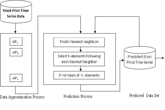
Figure 1: System Architecture

6 MATHEMATICAL MODEL AND ALGORITHM

6.1 Data Approximation Process

The given stock time series data $D$ of size $N$ is divided into number of equal partitions, $P_{1}$, $P_{2}$, …, $P_{n}$ and the total number of partitions is given by

$$n=N/K$$ (3)

where, $K$ is size of each partition. For each partition $P_{i}$, where $1\leq$ i $\leq$ K, segment $P_{i}$ into $n_{i}$ segments, $S_{1}$,…,$S_{n_{i}}$ and the total number of segments is given by,

$$n_{i}=|P_{k}|/t,$$ (4)

where, $t$ is size of each segment. The set of the segments for each partition $P_{i}$ is given by

$$S_{p_{i}}=[S_{1},S_{2},...,S_{n_{i}}]$$ (5)

The data approximation for the input stock time series data $D$ is obtained by computing the segments mean from $level$ $l$ to $level$ $0$ in the tree and the total number of levels in the tree is computed by following equation,

$$n_{l}=\log_{t}K$$ (6)

and at each $level$ $j$ we can form $(3^{l})$ disjoint segments, for each segment $S_{j}\in S_{p_{i}}$ in the $level$ l$=\log_{t}$K, mean of all the elements in $S_{i}$ is computed and stored in $AP_{ij}$[$l-1$]. The mean value in the [$l-1$] levels are grouped as one segment, again considering each segment in [$l-1$] level, find the mean of all elements in that segment and stored in $AP_{ij}$[$l-2$]. Similar procedure is followed to obtain $AP_{ij}$[$l-3$] upto $AP_{ij}$[$l-l$] $i.e.,$ $AP_{ij}$[$0$]. $AP_{ij}$[$0$] gives the approximated value of level $j$ for the partition $P_{i}$. This process is continued for computing the approximation for all the levels, finally, the approximated values are as follows,
$Ap$= [$Ap_{10}$, $Ap_{20}$, …, $Ap_{n0}$].
Figure 1 shows the segment mean representation of stock time series data $D$ of length $N$.

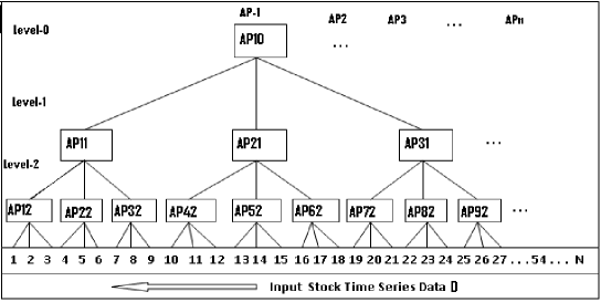
Figure 2: Data Approximation using $MSM$

Example: This example shows the computation of the approximation values for the given input stock time series data. In Figure 2, at $level$ 2, 1 and 0 we construct total of 9, 3 and 1 segments respectively. The first segment $AP_{12}$ at $level$ 2 is the mean of the $1^{st}$, $2^{nd}$ and $3^{rd}$ value in the input stock time series data $D$. Similarly, the second segment $AP_{22}$ at $level$ 2 is the mean of the $4^{th}$, $5^{th}$ and $6^{th}$ values in the input stock time series data $D$. So we can construct the segments upto $AP_{92}$ on $level2$. $i.e.,$ $AP_{12}$, $AP_{22}$, $AP_{32}$ …, $AP_{92}$ as shown in Figure 2.
At $level$ 1, we construct 3 segments $AP_{11}$, $AP_{21}$ and $AP_{31}$ as follows:
The segment $AP_{11}$ is computed by the mean of 3 adjacent segments on $level$ 2, $i.e.$, $AP_{11}$=[$AP_{12}$ + $AP_{22}$ + $AP_{32}$]/3, $AP_{21}$=[$AP_{42}$ + $AP_{52}$ + $AP_{62}$]/3 and $AP_{31}$=[$AP_{72}$ + $AP_{82}$ + $AP_{92}$]/3. Lastly, we can compute the only one segment $AP_{10}$ at $level$ $0$ as follows,
$AP_{10}$=[$AP_{11}$ + $AP_{21}$ + $AP_{31}$]/3. Hence $AP_{10}$ is the approximated value of the first group $K_{1}$ in the input stock time series data $D$, $i.e.$, $AP_{1}$=$AP_{10}$. In the same manner, we can compute another approximated value $AP2$ from the next partition $K_{2}$ and next approximatd value $AP3$ from the next partition $K_{3}$ and so on. The set of approximated values at $level$ $0$, are formed as follows, $Ap$= [$Ap_{10}$, $Ap_{20}$, …, $Ap_{n0}$]

6.2 Prediction Process

The Stock price time series values are predicted using the data approximation values obtained in the previous section.

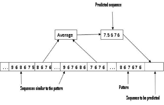
Figure 3: Prediction Process using Nearest Neighbour

Given the set of approximated values as $Ap={Ap_{1},Ap_{2},\ldots,Ap_{n}}$ and we need to compute a set of predicted values as follows,

$$P^{\prime}={v_{1},v_{2},\ldots,v_{m}}$$ (7)

Let $W$ be the window of size $w$, and $m$ be the size of the predicted values, in our case $m$=1. Now consider the last $w$ elements in the input sequence $Ap$, $i.e.$, pattern set $PS$ and is given by,

$$PS={AP_{n-w},AP_{n-w-1},\ldots,AP_{n-1},AP_{n}}$$ (8)

Next, the nearest neighbour in $AP$ is obtained for $PS$. Let $k$ be number of nearest neighbours in $AP$. In $PS$, the set of nearest neighbour is given by,

$$NN={nn_{1},nn_{2},\ldots,nn_{k}}$$ (9)

For each nearest neighbour, $nn_{i}\in NN$, retrive sequence of $m$ elements next to $nn_{i}$ $i.e,$.

$$EL_{i}={e_{i1},e_{i2},\ldots,e_{im}}$$ (10)

are the sequence of elements next to $nn_{i}$. Set of sequence of $m$ elements next to all the nearest neighbours in $NN$ is given by the set $NS$.

$$NS=EL_{1},EL_{2},\ldots EL_{k}$$ (11)

The predicted value in the sequence, that consists of average of corresponding elements in the set $NS$ is given by,
$P^{\prime}<{v_{1},v_{2},\ldots,v_{m}}>=$

$${\frac{1}{k}{\sum_{i=1}^{k}E_{i1}},\frac{1}{k}{\sum_{i=1}^{k}E_{i2}},\ldots,\frac{1}{k}{\sum_{i=1}^{k}E_{im}}}$$ (12)

Example: Prediction process is shown in the Figure 3. Table 1 shows the complete algorithm for Data approximation and Prediction of Stock time series data.

Table 1: Algorithm :$APST$: Approximation and Prediction of Stock Time-Series Data

$\mathbf{Algorithm:}$ $\mathbf{\it APST(D,~{}K,~{},t~{},w,~{}m)}$

Input: $D$ : Stock time series data set of size $N$

$k$ : Size of each partition

$t$ : Size of each segment

$w$ : Window size

$m$ : Size of sequence to predicted

Output: $P^{\prime}$ : Predicted Stock values

———————————————————————————————-

Phase-1: $Data$ $Approximation$

———————————————————————————————-

begin

$N=1$, $n=N/K$, $l=\log_{t}k$;

$P$= Partition $D$ into $p_{1}$, $p_{2}$, …, $p_{n}$ of size $k$

for each partition $p_{i}$ $\in$ $P$ do

Segment $p_{i}$ into $n_{i}$ segments $s_{1}$, $s_{2}$, …, $s_{ni}$

$S_{P_{i}}$=$s_{1}$, $s_{2}$, …, $s_{n}$

for each Segment $S_{j}$ $\in$ $S_{P_{i}}$ do

$AP_{ij}[l-1]$=Mean of each elements in $S_{j}$

end for

end for

for $l=(\log_{t}k,l\geq 0,l--)$ do

Groups the elements in $AP_{ij}[l-1]$ into segments of $t$ elements

for each segment find the mean and store in $AP_{ij}[l-2]$

repeating the same steps to find the mean upto $AP_{ij}[l-l]$

end for

end

//The final set of approximation values for all the levels are,

//$AP_{ij}[l-l]$ = $AP_{ij}[0]$ = $Ap$= [$Ap_{10}$, $Ap_{20}$, …, $Ap_{n0}$]

//These values are used in the Phase-2 for the Prediction.

———————————————————————————————

Phase-2: $Data$ $Prediction$

———————————————————————————————-

begin

$Ap$= [$Ap_{10}$, $Ap_{20}$, …, $Ap_{n0}$]

$PS=<{AP_{n-w},AP_{n-w-1},\ldots,AP_{n-1},AP_{n}}>$

$NN$= Find the nearest neighbours for $PS$ in $AP$ $<{nn_{1},nn_{2},\ldots,nn_{k}}>$

for each $nn_{i}$ $\in$ $NN$ do

$E_{i}$= Extract Sequence $<{e_{i1},e_{i2},\ldots,e_{im}}>$ of $m$ elements next to $nn_{i}$

end for

for each $j$=1 to $m$ do

for each Element $E_{i}$ $\in$ $E$ do

$P^{\prime}[j]$=$P^{\prime}[j]$+$e_{ij}$

end for

end for

end

The aproximated values are extracted from the stock time series data $D$. Considering the patterns of length $w$ in the aproximated values, we have to predict a stock sequence of the next time step. In the prediction process, search for $k$ nearest neighbors stock values within the threshold $\psi$ of that pattern and then the stock sequences next to the found neighbors are extracted. The predicted stock sequence is then estimated by taking the mean of the sequences found in the previous step. The computational cost of our proposed $APST$ method, for data approximation is $O(n*n_{i})$. Where, $n$ is the number of partitions and $n_{i}$ is the number of segments. The computational cost of prediction task is $O(m*|NN|)$. Where, $m$ is the size of sequence to be predicted and $|NN|$ is the total size of the nearest neighbours. Thus, the accuracy and the time required for prediction in the proposed method is comparatively efficient than the existing Label Based Forecasting ($LBF$) method.

7 EXPERIMENTAL RESULTS

Experiments are conducted on two real datasets, TAIiwan stock EXchange index dataset (TAIEX) and Bombay Stock EXchange index dataset (BSEX) for different companies. The performance of our prediction approach is compared with that of $LBF$ method. We use Mean Error Relative ($MER$) and Mean Absolute Error ($MAE$) for evaluation which are defined as follows [1].

$$MeanErrorRelative=100{\frac{1}{N}}\sum_{d=1}^{N}\frac{|{P^{\prime}}-{P}|}{\bar{P}}$$ (13)

Where, $P^{\prime}$ is the predicted stock prices at particular day ‘$d$’. $P$ is the current stock prices for particular day ‘$d$’. $\bar{P}$ is the mean stock prices for the period of interest(day/week). $N$ is the number of predicted days

$$MeanAbsoluteError={\frac{1}{N}}\sum_{d=1}^{N}|{P^{\prime}}-{P}|$$ (14)

Table 2: The Prediction Errors by $LBF$ and $APST$ methods on the TAIEX dataset for the financial year 2010

Month	MER($LBF$)	MER($APST$)	MAE($LBF$)	MAE($APST$)
April	5.02	4.22	0.53	0.43
May	8.30	7.22	0.56	0.46
June	6.89	5.59	0.51	0.41
July	7.41	6.21	0.47	0.37
Aug	8.37	7.57	0.47	0.37
Sep	7.30	6.40	0.45	0.35
Oct	4.62	3.68	0.47	0.37
Nov	7.26	6.28	0.44	0.34
Dec	6.88	5.88	0.43	0.35
Jan	7.20	8.26	0.44	0.36
Feb	6.26	4.26	0.44	0.35
Mar	7.26	5.26	0.44	0.38

Using the above two equations, we compute $MER$ and $MAE$ for both the existing $LBF$ method and proposed $APST$ method for the TAIEX dataset and shown in the Table 2 and Table 3. From Table 2 and 3, it shows that the average MER is 6.89%, Average MAE is 0.47% in the existing $LBF$ method, whereas in the proposed $APST$ method, the average $MER$ is 5.90% and Average $MAE$ is 0.37% . The proposed $APST$ method is $\approx$ 1% more efficient with respect to $MER$ and 0.1 % more efficient for $MAE$ compared to existing $LBF$ method.

Table 3: Performance of $LBF$ and $APST$ with Respect to $MER$ and $MAE$

	AVG.MER	AVG.MAE
$LBF$	6.89	0.47
$APST$	5.90	0.37

The graphs shown in Figures 4 and 5, indicates that, the prediction accuracy of our proposed $APST$ method is better than that of the existing $LBF$. The graph is plotted by taking the actual stock price values against the predicted stock price values for both the methods. The graph shown in Figure 6, indicates that, the average CPU time required to forecast diferent stock timeseries data. We observed that, the average CPU time required for existing $LBF$ method is 0.61 miliseconds. Whereas in our proposed $APST$ method, the average CPU time required is 0.5 miliseconds. Our technique $APST$ is 0.11% more efficient than the existing $LBF$ method because, in $LBF$ they consider the entire data set $N=|D|$, whereas in $APST$ we consider the approximated data set, $n=|AP|$ ${i.e.,}$ Size of data in $APST$=$(N/n)$. Time complexity of $LBF$ is $O(No.ofdays*|E_{s_{d}}|)$, whereas in $APST$ time complexity is $O(m*|NN|)$, and number of subsequences in $APST$ is less than the $E_{s_{d}}$ in $LBF$.

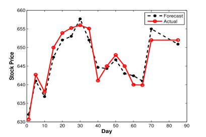
Figure 4: Comparison between Actual value and Forecasted value in $LBF$ method

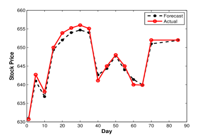
Figure 5: Comparison between Actual value and Forecasted value in $APST$ method

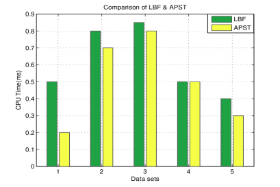
Figure 6: Comparison of Forecasting Time between $LBF$ and $APST$ methods

8 CONCLUSIONS

The proposed mechanism $APST$ works in two phase process. In the first phase we perform data approximation using Multiscale Segment Mean($MSM$) approach to get the approximated values of the given stock time series data. In the second phase, the prediction of stock time series is carried out using the Euclidian distance and the Nearest Neighbour approach. The computational cost of proposed method with respect to data approximation is $O(n*n_{i})$ and for the prediction task is $O(m*|NN|)$ respectively. Further, our experimental results show that the average MER is 6.89%, average MAE is 0.47% in the existing $LBF$ method, whereas in the proposed method, the average $MER$ is 5.90% and average $MAE$ is 0.37%. Thus, the proposed method is $\approx$ 1% more efficient with respect to $MER$ and 0.1 % more efficient for $MAE$ compared to existing $LBF$ method. Also, the average CPU time required for existing $LBF$ method is 0.61 miliseconds, whereas in the proposed method, it is 0.5 miliseconds. Thus, proposed method is 0.11% more efficient than the existing method. Future enhancement can be focused on selecting the window size dynamically and fine tune the matching sequence.

Vishwanath R Hulipalled is an Assistant Professor in the Department of Computer Science and Engineering at Sambhram Institute of Technology, Bangalore, India. He received his Bachelors degree in Computer Science and Engineer

ing from Karnataka University and Master of Engineering from UVCE, Bangalore University, Bangalore. He is presently pursuing his Ph.D in the area of Data Mining in JNTU Hyderabad. His research interest includes Time Series Mining and Data Analysis.

Leena is pursuing B.E in Department of Computer Science and Engineering, University Visveswaraya College of Engineering, Bangalore. Her research interest is in the area of Data Mining and Time Series Mining.

Srikantaiah K C is an Associate Professor in the Department of Computer Science and Engineering at S J B Institute of Technology, Bangalore, India. He obtained his B.E and M.E degrees in Computer Science and Engineering from Bangalore University, Bangalor-

e. He is presently pursuing his Ph.D programme in the area of Web Mining in Bangalore University. His research interest is in the area of Data Mining, Web Mining and Semantic Web.

K Shreekrishna Kumar is currently the Director of All India Council for Technical Education, SWRO, Bangalore. He obtained his Master of Science from Bhopal University. He received his Masters degree in Information Technology from Punjab University. He was awa

rded Ph.D in Physics (Glass Technology) from Mahatma Gandhi University. He was the member of the Jury Panel, Indian Journal of Pure and Applied Physics, CSIR (New Delhi), He was the Collaborative researcher, Nuclear Science Centre, New Delhi.

P Deepa Shenoy was born in India, on May 9, 1961. She graduated form UVCE, completed her M.E. from UVCE., has done her MS(Systems and information) from BITS., Pilani, and has obtained her Ph.D in CSE from Bangalore

University. She is presently employed as a Professor in department of CSE at UVCE. Her research interests include Computer Networks, Wireless Sensor Networks, Parallel and Distributed Systems, Digital Signal Processing and Data Mining.

Venugopal K R is currently the Principal, University Visvesvaraya College of Engineering, Bangalore University, Bangalore. He obtained his Bachelor of Engineering from University Visvesvaraya College of Engineering. He received his Masters degree in Computer Science and

Automation from Indian Institute of Science Bangalore. He was awarded Ph.D in Economics from Bangalore University and Ph.D in Computer Science from Indian Institute of Technology, Madras. He has a distinguished academic career and has degrees in Electronics, Economics, Law, Business Finance, Public Relations, Communications, Industrial Relations, Computer Science and Journalism. He has authored and edited 39 books on Computer Science and Economics, which include Petrodollar and the World Economy, C Aptitude, Mastering C, Microprocessor Programming, Mastering C++ and Digital Circuits and Systems $etc.$. During his three decades of service at UVCE he has over 350 research papers to his credit. His research interests include Computer Networks, Wireless Sensor Networks, Parallel and Distributed Systems, Digital Signal Processing and Data Mining.

S S Iyengar is currently the Roy Paul Daniels Professor and Chairman of the Computer Science Department at Louisiana State University. He heads the Wireless Sensor Networks Laboratory and the Robotics Research Laboratory at LSU.

He has been involved with research in High Performance Algorithms, Data Structures, Sensor Fusion and Intelligent Systems, since receiving his Ph.D degree in 1974 from MSU, USA. He is Fellow of IEEE and ACM. He has directed over 40 Ph.D students and 100 Post Graduate students, many of whom are faculty at Major Universities worldwide or Scientists or Engineers at National Labs/Industries around the world. He has published more than 500 research papers and has authored/co-authored 6 books and edited 7 books. His books are published by John Wiley & Sons, CRC Press, Prentice Hall, Springer Verlag, IEEE Computer Society Press $etc.$. One of his books titled Introduction to Parallel Algorithms has been translated to Chinese.

L M Patnaik is currently Honorary Professor, Indian Institute of Science, Bangalore, India. He was a Vice Chancellor, Defense Institute of Advanced Technology, Pune, India and was a Professor since 1986 with the Department of Computer Science and Automation, Indian

Institute of Science, Bangalore. During the past 35 years of his service at the Institute he has over 700 research publications in refereed International Journals and refereed International Conference Proceedings. He is a Fellow of all the four leading Science and Engineering Academies in India; Fellow of the IEEE and the Academy of Science for the Developing World. He has received twenty national and international awards; notable among them is the IEEE Technical Achievement Award for his significant contributions to High Performance Computing and Soft Computing. His areas of research interest have been Parallel and Distributed Computing, Mobile Computing, CAD for VLSI circuits, Soft Computing and Computational Neuroscience.

References

- [1] F Martınez-Alvarez, A Troncoso, J C Riquelme and J S Aguilar Ruiz. LBF: A Labeled-Based Forecasting Algorithm and Its Application to Electricity Price Time Series, in Proceedings of Eighth IEEE Int’l Conf. Data Mining, pages 453–461, 2008.
- [2] Xiang Lian, Lei Chen, Jeffrey Xu Yu, Jinsong Han, Jian Ma. Multiscale Representations for Fast Pattern Matching in Stream Time Series, in IEEE Transaction on Knowledge and Data Engineering, 21(4):568–581, 2009.
- [3] A Troncoso, J C Riquelme, J M Riquelme, J L Martınez and A Gomez. Electricity Market Price Forecasting Based on Weighted Nearest Neighbours Techniques, in IEEE Transaction on Power Systems, 22(3):1294–1301, 2007.
- [4] K J Kim. Financial Time Series Forecasting using Support Vector Machines, in Neuro-Computing, 55:307–319, 2003.
- [5] Y Radhika and M Shashi. Atmospheric Temperature Prediction using Support Vector Machines, in International Journal of Computer Theory and Engineering, 1:55–58, 2009.
- [6] R Nayak and te Braak. Temporal Pattern Matching for the Prediction of Stock Prices, in Proceedings of 2nd International Workshop on Integrating Artificial Intelligence and Data Mining (AIDM2007), pages 99–107, 2007.
- [7] A J Conejo, M A Plazas, R Espınola and B Molina. Day-Ahead Electricity Price Forecasting Using the Wavelet Transform and Models, in IEEE Transaction on Power Systems, 20:1035–1042, 2005.
- [8] Akinwale Adio T, Arogundade O T and Adekoya Adebayo F. Translated Nigeria Stock Market Price using Artificial Neural Network for Effective Prediction, in Journal of Theoretical and Applied Information Technology, 2009.
- [9] Kuang Yu Huang and Chuen-Jiuan Jane. A Hybrid Model Stock Market Forecasting and Portfolio Selection Based on ARX, Grey System and RS Theories, in Expert Systems with Applications, pages 5387–5392, 2009.
- [10] M Suresh babu, N Geethanjali and B Sathyanarayana. Forecasting of Indian Stock Market Index Using Data Mining and Artificial Neural Nework, in International journal of Advance Engineering and Application, 2011.
- [11] F M Álvarez, A Troncoso, J C Riquelme and J S A Ruiz. Energy Time Series Forecasting Based on Pattern Sequence Similarity, in IEEE Transcation on Knowledge and Data Engineering, 23(8):1230–1243, 2011.
- [12] Vishwanath R H, Leena S V, Srikantaiah K C, K Shreekrishna Kumar, P Deepa Shenoy, Venugopal K R, S S Iyengar and L M Patnaik. : Approximation and Prediction of Stock Time-Series Data using Pattern Sequence, in Proceedings 8th International Multi Conference on Information Processing (ICIP2013), 2013.