Optimization of an Amplification Protocol for Misfolded Proteins by using Relaxed Control

Abstract

We investigate an optimal control problem which arises in the optimization of an amplification technique for misfolded proteins. The improvement of this technique may play a role in the detection of prion diseases. The model consists in a linear system of differential equations with a nonlinear control. The appearance of oscillations in the numerical simulations is understood by using the Perron and Floquet eigenvalue theory for nonnegative irreducible matrices. Then to overcome the unsolvability of the optimal control, we relax the problem. In the two dimensional case, we solve explicitly the optimal relaxed control problem when the final time is large enough.

Keywords: optimal control, relaxed control, turnpike, Pontryagin maximum principle, Perron eigenvalue, Floquet eigenvalue, structured populations.

2010 Mathematics Subject Classification. 49J15, 35Q92, 37N25.  

1 Introduction

Transmissible Spongiform Encephalopathies (TSE) are fatal, infectious, neurodegenerative diseases. They include bovine spongiform encephalopathies (BSE) in cattle, scrapie in sheep and Creutzfeldt-Jakob disease (CJD) in human. During the so-called “mad-cow crisis” in the 90’s, people were infected by a variant of BSE by ingesting contaminated pieces of beef. More recently, CJD was transmitted between humans via blood or growth hormones. Because of the long incubation times (some decades), TSE still represent an important public health risk. There is no ante mortem diagnosis currently available to detect infected individuals and prevent possible contaminations. A promising tool to design a diagnosis test is the protein misfolded cyclic amplification (PMCA) technique [7, 29, 30].

The PMCA principle is based on the “protein-only hypothesis” [16, 27]. According to this widely accepted hypothesis, the infectious agent of TSE, known as prions, may consist in misfolded proteins called PrPsc (for Prion Protein scrapie). The PrPsc replicates in a self-propagating process, by converting the normal form of PrP (called PrPc for Prion Protein cellular) into PrPsc. The PMCA enabled to consolidate the idea of an autocatalytic replication of PrPsc by nucleated polymerization. In this model originally proposed by Landsbury [17], PrPsc is considered to be a polymeric form of PrPc. Polymers can lengthen by addition of PrPc monomers, and they can replicate by splitting into smaller fragments. The PrPc is mainly expressed by the cells of the central nervous system, so PrPsc concentrates in this zone. The amount of PrPsc in tissues such as blood is very small and this is why it is very difficult to diagnose an infected individual.

The PMCA mimics in vitro the nucleation/polymerization mechanism occurring in vivo with the aim to quickly amplify the polymers present in minute amount in an infected sample. It is a cyclic process, where each cycle consists in two phases: the incubation phase during which the polymerization is favored due to the presence of a large quantity of PrPc monomers, and the sonication phase when the PrPsc polymers are broken down with ultrasounds. The incubation phase is expected to increase the size of the polymers, while the ultrasounds are known to increase the fragmentation of the polymers and so increase their number. This technique could allow us to detect PrPsc in the samples of blood for instance. But for now, it is not efficient enough to do so. Mathematical modelling and optimization tools can help to optimize the PMCA protocol.

The mathematical modeling of prion proliferation with ordinary or partial differential equation (PDE) produced a large literature since the first model of Griffith [16]. Today, the most widely studied nucleation/polymerization model is the one of Masel [24]. A PDE version of this model has been introduced by Greer et al. [15] and studied by many authors including [5, 6, 10, 12, 13, 18, 28, 32, 36]. Starting from it, we propose to model the PMCA with the following controlled size-structured PDE

$$\partial_{t}f(t,\xi)+r(u(t))\partial_{\xi}\bigl{(}\tau(\xi)f(t,\xi)\bigr{)}=u(t)\left(\int_{\xi}^{\infty}\beta(\zeta)\kappa(\xi,\zeta)f(t,\zeta)\,d\zeta-\beta(\xi)f(t,\xi)\right)$$ (1.1)

with the boundary condition $f(t,0)=0$ for every time $t\geq 0$. The unknown $f(t,\xi)$ is the number, or density of polymers of size $\xi>0$ at time $t$. The size of the polymers increases by polymerization with respect to the individual growth rate $\tau(\xi)$. The terms in the large brackets on the right-hand side of (1.1) form the fragmentation operator, with $\beta(\xi)$ the global fragmentation rate and $\kappa(\xi,\zeta)$ the fragmentation kernel. The conservation of the quantity of polymerized proteins during the fragmentation process requires that this kernel satisfies the following standard condition (see [9] for instance)

$$\int_{0}^{\zeta}\xi\,\kappa(\xi,\zeta)\,d\xi=\zeta.$$ (1.2)

The fragmentation is modulated by a multiplicative factor $u(t)\in[u_{\min},u_{\max}]$ which represents the sonication intensity. The control $u(t)\equiv u_{\min}=1$ corresponds to the absence of sonication, while $u(t)\equiv u_{\max}>1$ represents the maximal power of the sonicator. We assume that the sonication does not only increase the fragmentation but also influence the polymerization process. This is taken into account by the positive term $r(u(t))$ where the function $r$ should be decreasing if we consider that the ultrasounds have a negative effect on the growth of the polymers. The optimal control problem we are interested in is, starting with a given initial size distribution $f(t=0,\xi)=f^{0}(\xi)\geq 0$, to maximize the objective

$$J(u)=\int_{0}^{\infty}\xi f(T,\xi)\,d\xi,$$ (1.3)

which represents the total quantity of polymerized proteins at a given final time $T$.

For the mathematical study in this paper, we consider a $n$-compartment approximation of (1.1)

$$\dfrac{dx_{i}}{dt}+r(u(t))(\tau_{i}x_{i}-\tau_{i-1}x_{i-1})=u(t)\left(\sum_{j=i+1}^{n}\beta_{j}\,\kappa_{i,j}\,x_{j}-\beta_{i}x_{i}\right)\ ,\quad\mbox{for}\ 1\leq i\leq n,$$

with $\beta_{1}=0$ and $\tau_{n}=0$. This is a finite dimensional ordinary differential system, linear in $x=(x_{1},\dots,x_{n})^{T}$, which can be written under a matrix form

$$\left\{\begin{array}[]{l}\dot{x}=uFx+r(u)Gx,\qquad t\in[0,T],\vspace{2mm}\\ x(t=0)=x^{0}>0,\end{array}\right.$$ (1.4)

where $G$ is the growth matrix

$$G=\left(\begin{array}[]{ccccc}-\tau_{\text{\scriptsize$1$}}&&&&\\ \tau_{\text{\scriptsize$1$}}&-\tau_{\text{\scriptsize$2$}}&&\text{\LARGE$0$}&\\ &\ddots&\ddots&&\\ &&&&\\ &\text{\LARGE$0$}&\tau_{\text{\scriptsize$n-2$}}&-\tau_{\text{\scriptsize$n-1$}}&\\ &&&\tau_{\text{\scriptsize$n-1$}}&0\end{array}\right),$$ (1.5)

and $F$ is the fragmentation matrix

$$F=\left(\begin{array}[]{cccc}0&&&\\ &-\beta_{2}&&\text{{\Large$(\kappa_{ij}\beta_{j})_{i<j}$}}\\ &&\ddots&\\ &\text{\LARGE$0$}&&\\ &&&-\beta_{n}\end{array}\right).$$ (1.11)

In (1.4) and in the following, if $x=(x_{1},\dots,x_{n})^{T}$, by $x>0$ (and we also write $x$ is positive) we mean that $x_{i}>0$ for every $i\in\{1,\cdots,n\}.$ We use the same notation for row vectors.

We assume that

$$\tau_{i}>0\quad\text{and}\quad\beta_{i+1}>0,\qquad\forall i\in[1,n-1].$$ (1.12)

The mass conservation assumption (1.2) on $\kappa$ becomes

$$\sum_{i=1}^{j-1}i\,\kappa_{ij}=j,\qquad j=2,\cdots,n.$$ (1.13)

The quantity (1.3) we want to maximize writes

$$J(u)=\sum_{i=1}^{n}i\,x_{i}(T).$$ (1.14)

Such $n$-compartment optimal control problems have been widely studied in cancer chemotherapy and the conclusion is usually that the optimal control is bang-bang since singular controls are not optimal [19, 20, 21, 22, 33]. In contrast with these results, we show that, for our problem, the optimal control is essentially singular.

The organization of the paper is the following. In Section 2, we investigate eigenvalue optimization problems related to the optimal control problem (1.14). More precisely we maximize the Perron eigenvalue with respect to constant control parameters and compare the maximum to Floquet eigenvalues, which are the analogue of Perron eigenvalues for periodic coefficients. We remark that fast oscillating controls can provide a greater Floquet eigenvalue than the optimal Perron eigenvalue. This observation indicates that a classical optimal control may not exist and motivates the relaxation of the problem. The relaxed control problem, for which the set of controls is extended to its convex hull, is investigated in Section 3. We prove that the trajectories corresponding to the constant control which maximizes the Perron eigenvalue in the new convex set satisfy the Pontryagin Maximum Principle (see Proposition 8). In Section 4, we state and prove the main result of the paper (Theorem 18) which treats the case of the two-compartment model: for $n=2$ the optimal relaxed control is unique and can be computed explicitly. Except for initial and terminal times, i.e., $t$ close to $0$ or close to $T$, this optimal control is equal to the constant which maximizes the Perron eigenvalue. Finally, in the Appendix, we give the details of the proofs for the results of Section 2.

2 Eigenvalue problems

For a fixed parameter $u>0$ and for $r(u)>0,$ the matrix $uF+r(u)G$ is irreducible (see, for instance, [31, Section 2.8] for a definition of irreducible) and has nonnegative extra-diagonal entries. So the Perron-Frobenius theorem (see, for instance, [31, Section 5.3]) applies and ensures the existence of a simple dominant eigenvalue $\lambda_{P}$. In our case, this eigenvalue is positive and it provides the exponential growth rate of the solutions to the equation $\dot{x}=(uF+r(u)G)x$ (see, for instance, [26, Section 6.3.1]). A first question is to investigate the dependence of the first eigenvalue on the parameter $u$. Maximizing the Perron eigenvalue is related to our optimal control problem (1.14). It can be regarded as the limit when $T\to+\infty$ of our optimization problem when we restrict to constant controls. A remarkable fact is that for some coefficients, the dependence $u\mapsto\lambda_{P}(u)$ can be non monotonic and there may exist an optimal value $u_{\mathrm{opt}}$ for which $\lambda_{P}$ admits a global maximum on $\mathbb{R}^{+}$. Theorem 1, which is proved in Appendix A, gives sufficient conditions for the existence of such a global optimum.

Theorem 1.

Assume that $r:\mathbb{R}^{+}\to\mathbb{R}^{+*}$ is continuous and admits an expansion of the form

$$\exists\,l>0,\,r_{l}\geq 0,\qquad r(u)=r_{0}+r_{l}u^{-l}+\underset{u\to+\infty}{o}\left(u^{-l}\right).$$ (2.1)

Consider also that $(\tau_{i})_{1\leq i\leq n}$ satisfies the condition

$$\exists\,k\in\mathbb{N}^{*}\quad\text{such that}\quad\forall\,i\leq k,\ \tau_{i}=i\,\tau_{1}\quad\text{and}\quad\tau_{k+1}>(k+1)\tau_{1}.$$ (2.2)

Then there exists an optimal value $u_{\mathrm{opt}}>0$ which satisfies

$$\forall\,u\geq 0,\qquad\lambda_{P}(u)\leq\lambda_{P}(u_{\mathrm{opt}}).$$

The interpretation is that in this case, there is a compromise between too much sonication which forms many small polymers but may have a small growth rate, and too high sonication which forms large polymers but in small quantity.

The theory of Perron-Frobenius can be extended to periodic controls: this is the Floquet theory. It ensures that for time periodic matrices which are monotonic and irreducible for any time, there exists a dominant eigenvalue. It allows one to define for a periodic control $u(t)$ a Floquet eigenvalue $\lambda_{F}[u]>0$ which prescribes, as in the case of the Perron eigenvalue, the asymptotic exponential growth rate of the solutions to the equation $\dot{x}=(u(t)F+r(u(t))G)x$ (see [26, Section 6.3.2] for instance). A natural question is then to compare these periodic eigenvalues to the best constant one $\lambda_{P}(u_{\mathrm{opt}})$. Theorem 2, which is proved in Appendix B, ensures that if $r$ satisfies the condition

$$\frac{r^{\prime\prime}(u_{\mathrm{opt}})}{r(u_{\mathrm{opt}})-u_{\mathrm{opt}}\,r^{\prime}(u_{\mathrm{opt}})}>0,$$ (2.3)

then the value $u_{\mathrm{opt}}$ is a saddle point in the set of periodic controls. This means that there exist periodic controls which provide a larger growth rate than $\lambda_{P}(u_{\mathrm{opt}})$.

Theorem 2.

Assume that there exists an optimal value $u_{\mathrm{opt}}$ for the Perron eigenvalue and that $u_{\mathrm{opt}}F+r(u_{\mathrm{opt}})G$ is diagonalizable. Define for a frequency $\omega>0$ and a perturbation $\varepsilon>0$ the Floquet eigenvalue $\lambda_{F}(\varepsilon,\omega):=\lambda_{F}[u_{\mathrm{opt}}+\varepsilon\cos(\omega t)]$. Then we have

$$\lim_{\omega\to+\infty}\frac{\partial^{2}}{\partial\varepsilon^{2}}\lambda_{F}(0,\omega)=\frac{1}{2}\,\frac{r^{\prime\prime}(u_{\mathrm{opt}})}{r(u_{\mathrm{opt}})-u_{\mathrm{opt}}\,r^{\prime}(u_{\mathrm{opt}})}\,\lambda_{P}(u_{\mathrm{opt}}).$$

The computation of second order approximation of the Floquet eigenvalue is used to detect “resonance” in population models with periodic coefficients (see [1] and the references therein). For these models, resonance is said to occur if periodic variations in the coefficients increase the growth rate.

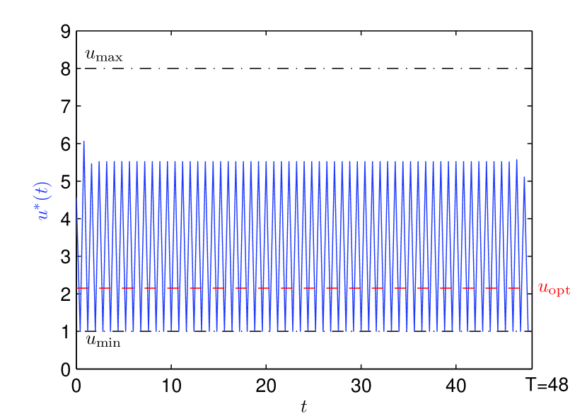
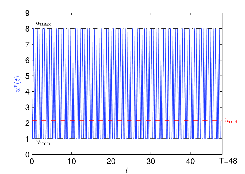
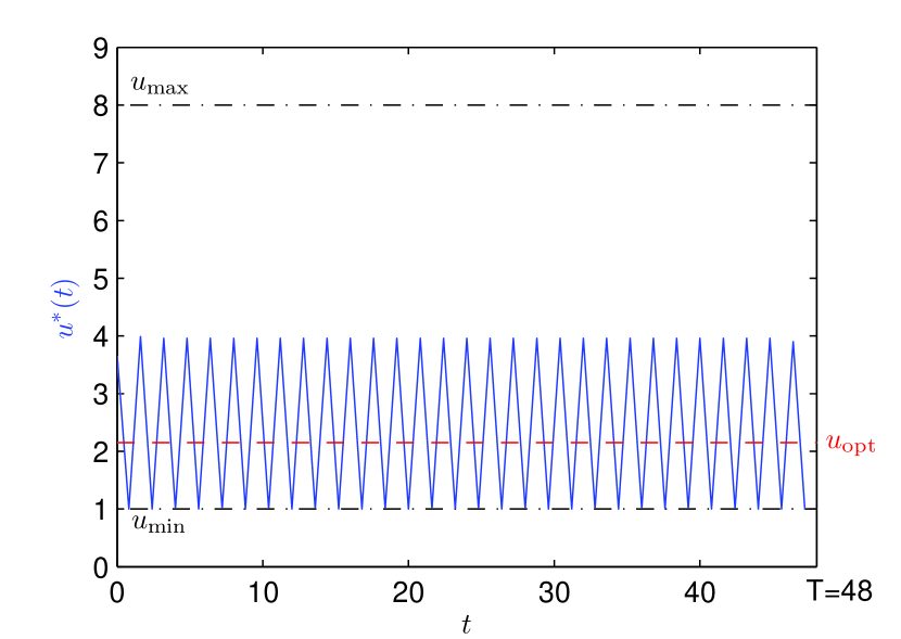
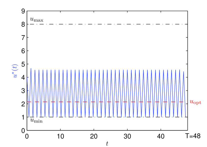
The link between the eigenvalue problem and the optimal control problem (1.14) is investigated in [4] when the function $r$ is a constant. In this case, there exists an optimal control $u^{*}(t)$ which is essentially equal to the best constant $u_{\mathrm{opt}}$ of the Perron optimization problem (see Chapter 5 in [12] for numerical simulations). Under condition (2.3) and the assumptions of Theorem 2, such a behavior is not expected since we can find oscillating controls which provide a better eigenvalue than $u_{\mathrm{opt}}$. The aim of this paper is to investigate the optimal control problem (1.14) in the case where there exists an optimal constant $u_{\mathrm{opt}}\in(u_{\min},u_{\max})$ and the function $r$ satisfies Assumption (2.3). The first question is the existence of an optimal control since the numerical simulations in Figure 1 show oscillations. These questions are investigated in the following section by using the relaxed control theory.

Figure 1: Piecewise optimal controls $u^{*}(t)$ obtained for different values of $\Delta t$ with the decreasing convex function $r(u)=\frac{2}{1+u}.$ The control varies between $u_{\min}=1$ and $u_{\max}=8$ and the final time is $T=48.$ The dimension of the model is $n=3$ and the coefficients are $\tau_{1}=1,$ $\tau_{2}=10,$ $\beta_{2}=0.5,$ $\beta_{3}=1,$ $\kappa_{1,2}=2$ and $\kappa_{1,3}=\kappa_{2,3}=1.$ The time step varies as follows: $\Delta t=0.8$ (top left), $\Delta t=0.6$ (top right), $\Delta t=0.4$ (bottom left) and $\Delta t=0.2$ (bottom right).

3 Relaxed Control and the Pontryagin maximum principle

Let $u_{\min}$ and $u_{\max}$ be two positive real numbers such that $u_{\min}<u_{\max}$. We consider in this section a function $r\in\mathcal{C}^{2}([u_{\min},u_{\max}])$ satisfying

$$r(u)>0,\qquad\forall u\in[u_{\min},u_{\max}],$$ (3.1)

$$r^{\prime\prime}(u)>0,\qquad\forall u\in(u_{\min},u_{\max}),$$ (3.2)

$$r(u)-ur^{\prime}(u)>0,\qquad\forall u\in(u_{\min},u_{\max}),$$ (3.3)

and we assume that there exists a strict optimum $u_{\mathrm{opt}}\in(u_{\min},u_{\max})$ for the Perron eigenvalue. Under these assumptions, condition (2.3) is automatically fulfilled. Remark that condition (3.3) is satisfied when $r$ is decreasing and satisfies (3.1), which are relevant conditions from the viewpoint of biology. To study this case, it will be convenient to use the equivalent alternative statement of (1.4) where $x$ is solution to

$$\left\{\begin{array}[]{l}\dot{x}(t)=u(t)Fx(t)+v(t)Gx(t),\qquad t\in[0,T],\vspace{2mm}\\ x(t=0)=x^{0}>0,\end{array}\right.$$ (3.4)

with the two dimensional control $(u,v)$ which belongs to the graph of the function $r$, i.e.,

$$\forall\,t\in[0,T],\qquad(u(t),v(t))\in\Omega:=Graph(r)=\left\{(u,r(u)),\ u_{\min}\leq u\leq u_{\max}\right\}.$$

Let

$$\psi:=(1,2,\cdots,n)\in\mathbb{R}^{n}$$ (3.5)

be the mass vector. Note that, from (1.11), the mass conservation assumption (1.13) and (3.5), one has

$$\psi F=0.$$ (3.6)

The optimal control problem (1.14) now becomes

$$\text{maximize }J(u,v)=\psi x(T),\,(u,v):[0,T]\rightarrow\Omega\text{ is a Lebesgue measurable function},$$ (3.7)

subject to dynamics (3.4). Since the function $r$ is strictly convex, the graph $\Omega$ is not a convex subset of $\mathbb{R}^{2}$ and, since the kernel of $G$ is not reduced to $\{0\}$, for any $x>0$, the velocity set

$${\mathcal{V}}(x)=\{(uF+vG)x,\ (u,v)\in\Omega\}$$

is also not convex. For this kind of situation, the existence of an optimal control for (3.7) cannot be ensured and it is standard to relax the problem by replacing the control set $\Omega$ by its convex hull $Conv(\Omega)$ (see, for instance, [23, Section 4.2]). One replaces problem (3.7) by the following optimal control problem

$$\text{maximize }J(u,v)=\psi x(T),\,(u,v):[0,T]\rightarrow Conv(\Omega)\text{ is a Lebesgue measurable function},$$ (3.8)

subject to dynamics (3.4). For this problem, the velocity set is the convex hull of $\mathcal{V}(x)$, so it is convex and the existence of an optimal control is ensured by classical results (see [23, Theorem 5 p. 271] for instance). Moreover,

• The supremum in problem (3.7) is equal to the maximum in problem (3.8).

• Let $(u^{*},v^{*}):[0,T]\rightarrow Conv(\Omega)$ be a measurable function which is optimal for problem (3.8). Then one can easily construct a sequence of piecewise constant functions $(u^{n},v^{n})_{n\in\mathbb{N}}\rightarrow\Omega$ such that, for any $\varphi\in L^{\infty}(0,T)$,

  $$\int_{0}^{T}u^{n}\varphi\,dt\longrightarrow\int_{0}^{T}u^{*}\varphi\,dt\quad\text{ and }\int_{0}^{T}v^{n}\varphi\,dt\longrightarrow\int_{0}^{T}v^{*}\varphi\,dt\quad\text{as}\quad n\rightarrow+\infty.$$ (3.9)

  Let us emphasize that (3.9) implies that

  $$J(u^{n},v^{n})\rightarrow J(u^{*},v^{*})\text{ as }n\rightarrow+\infty.$$

  In particular, $(u^{n},v^{n})_{n\in\mathbb{N}}$ is a maximizing sequence for problem (3.7).

Now we want to obtain information on the optimal controls for (3.8) by using the Pontryagin maximum principle. This principle in our case gives the following theorem.

Theorem 3 (Pontryagin Maximum Principle (PMP)).

Let $(u^{*},v^{*})$ be an optimal control for problem (3.8) and let $x^{*}$ be the corresponding trajectory (i.e., the solution of (3.4) with $(u,v):=(u^{*},v^{*})$). Call $p^{*}:\,[0,T]\rightarrow\mathbb{R}^{n}$ the row vector solution of the adjoint linear equation

$$\dot{p}^{*}(t)=-p^{*}(t)(u^{*}F+v^{*}G),$$ (3.10)

with the transversality condition

$$p^{*}(T)=\psi.$$ (3.11)

Let us define the Hamiltonian as

$$H(x,p,u,v):=p(uF+vG)x.$$ (3.12)

Then the maximality condition

$$H(x^{*}(t),p^{*}(t),u^{*}(t),v^{*}(t))=\max_{(u,v)\in Conv(\Omega)}H(x^{*}(t),p^{*}(t),u,v)$$ (3.13)

holds for almost every time $t\in[0,T]$ and there exists a constant $H^{*}\in\mathbb{R}$ such that

$$H(x^{*}(t),p^{*}(t),u^{*}(t),v^{*}(t))=H^{*},\,\text{ for almost every }t\in[0,T].$$ (3.14)

Remark 4.

Since, for any positive $u$ and $v$, the matrix $uF+vG$ has nonnegative extra-diagonal entries, we have, using (3.4), (3.5), (3.10) and (3.11),

$$x^{*}(t)>0\quad\text{and}\quad p^{*}(t)>0,\quad\text{for every time}\quad t\in[0,T].$$ (3.15)

The Pontryagin maximum principle is useful to obtain information on the optimal control. It allows us to prove (Corollary 6 below) that the optimal control lies on the line $\Sigma$ defined by (see Figure 2)

$$\Sigma:=Graph(\sigma)=\left\{(u,\sigma(u)),\ u_{\min}\leq u\leq u_{\max}\right\},$$ (3.16)

where $\sigma$ is the affine function defined by

$$\sigma(u)=\theta u+\zeta$$

with

$$\theta:=\frac{r(u_{\max})-r(u_{\min})}{u_{\max}-u_{\min}},$$ (3.17)

$$\zeta:=\frac{u_{\max}r(u_{\min})-u_{\min}r(u_{\max})}{u_{\max}-u_{\min}}.$$ (3.18)

The set $\Sigma$ is the string which links $(u_{\min},r(u_{\min}))$ to $(u_{\max},r(u_{\max}))$. Since $r$ is convex, the boundary of the control set $Conv(\Omega)$ is $\partial Conv(\Omega)=\Omega\cup\Sigma$.

One has the following lemma which is illustrated by the incoming arrows in Figure 2.

Lemma 5.

Let $(u,v)\in Conv(\Omega)\setminus\Sigma$. Then, for $\varepsilon>0$ small enough,

$$((1+\varepsilon)u,(1+\varepsilon)v)\in Conv(\Omega).$$

\psfrag{Omega}[l]{$\Omega$}\psfrag{H(Omega)}[l]{$Conv(\Omega)$}\psfrag{Sigma}[l]{$\Sigma$}\psfrag{u}[l]{$u$}\psfrag{v}[l]{$v$}\psfrag{ru}[l]{$r(u)$}\includegraphics[width=238.49231pt]{convex_hull.eps}

Figure 2: The set $\Omega,$ the string $\Sigma$ and the convex hull $Conv(\Omega)$ for $r$ a decreasing and convex function. The arrows oriented along the vectors $(u,r(u))$ point inside $Conv(\Omega)$ on the lower boundary $\Omega.$

Proof of Lemma 5.

Let $Int(Conv(\Omega))$ be the interior of $Conv(\Omega)$. If $(u,v)\in Int(Conv(\Omega))$, then the result follows from the fact that $Int(Conv(\Omega))$ is an open set by definition. It remains to study the case where $(u,v)\in\Omega\setminus\{(u_{\min},r(u_{\min}))\}\cup\{(u_{\max},r(u_{\max}))\}$, i.e., $v=r(u)$ with $u\in(u_{\min},u_{\max})$. We have, using (3.3),

$$(1+\varepsilon)r(u)-r((1+\varepsilon)u) =(1+\varepsilon)r(u)-r(u)-\varepsilon ur^{\prime}(u)+\underset{\varepsilon\to 0^{+}}{o}(\varepsilon)$$

$$=\varepsilon(r(u)-u\,r^{\prime}(u)+\underset{\varepsilon\to 0^{+}}{o}(1))\geq 0,\quad\text{for $\varepsilon$ small and positive}.$$

Hence, if $\varepsilon>0$ is small enough, $r((1+\varepsilon)u)\leq(1+\varepsilon)r(u).$ Moreover, by (3.2), we have $r(u)<\sigma(u)$ and, therefore, if $\varepsilon$ is small enough, $(1+\varepsilon)r(u)\leq\sigma((1+\varepsilon)u)$.

The proof is complete. ∎

As a consequence of Theorem 3 and Lemma 5, we have the following corollary.

Corollary 6.

Let $(u^{*},v^{*})$ be an optimal control for problem (3.8). Then, for almost every time $t\in[0,T]$, the optimal control $(u^{*}(t),v^{*}(t))\in\Sigma$.

Proof of Corollary 6.

By (3.14), there exists a sequence $(t_{n})_{n\in\mathbb{N}}$ of elements in $[0,T]$ such that

$$H(x^{*}(t_{n}),p^{*}(t_{n}),u^{*}(t_{n}),v^{*}(t_{n}))=H^{*},$$ (3.19)

$$t_{n}\rightarrow T\quad\text{ as }\quad n\rightarrow+\infty.$$ (3.20)

Extracting a subsequence if necessary we may assume, without loss of generality, that there exists $\widetilde{v}\in\mathbb{R}$ such that

$$\widetilde{v}\in[r(u_{\max}),r(u_{\min})]\subset(0,+\infty),$$ (3.21)

$$v^{*}(t_{n})\rightarrow\widetilde{v}\quad\text{ as }\quad n\rightarrow+\infty.$$ (3.22)

Letting $n\rightarrow+\infty$ in (3.19), and using (3.6), (3.11), (3.12), (3.20) and (3.22), one gets that

$$H^{*}=\widetilde{v}\psi Gx(T).$$ (3.23)

From (1.5), (1.12) and (3.5), one gets that

$$\psi G>0,$$ (3.24)

which, together with (3.15), implies that

$$\psi Gx(T)>0.$$ (3.25)

From (3.21), (3.23) and (3.25), one obtains

$$H^{*}>0.$$

Let $t\in[0,T]$ be such that

$$(u^{*}(t),v^{*}(t))\in Conv(\Omega)\setminus\Sigma,$$ (3.26)

$$H(x^{*}(t),p^{*}(t),u^{*}(t),v^{*}(t))=H^{*}.$$ (3.27)

From Lemma 5 and (3.26), there exists $\varepsilon>0$ such that $((1+\varepsilon)u^{*}(t),(1+\varepsilon)v^{*}(t))\in Conv(\Omega)$. Using (3.27), one has

$$\begin{array}[]{rcl}H(x^{*}(t),p^{*}(t),(1+\varepsilon)u^{*}(t),(1+\varepsilon)v^{*}(t))&=&(1+\varepsilon)H(x^{*}(t),p^{*}(t),u^{*}(t),v^{*}(t))\\ &=&(1+\varepsilon)H^{*}\\ &>&H^{*}=H(x^{*}(t),p^{*}(t),u^{*}(t),v^{*}(t)),\end{array}$$

which shows that (3.13) does not hold. Since, by Theorem 3, (3.13) holds for almost every $t\in[0,T]$, this, together with (3.14), concludes the proof of Corollary 6. ∎

Now we look for controls and corresponding trajectories which satisfy the optimality condition (3.13). To that end, we take advantage of our analysis of the Perron eigenvalue problem. For $(u,v)\in Conv(\Omega)$, define the Perron eigenvalue $\lambda_{P}=\lambda_{P}(u,v)$ of the matrix $uF+vG$ and the corresponding right and left eigenvectors $X>0$ and $\phi>0$ normalized as follows

$$\lambda_{P}X=(uF+vG)X,\quad\|X\|_{1}=1,$$ (3.29)

$$\lambda_{P}\phi=\phi(uF+vG),\quad\phi X=1,$$ (3.30)

where, for $x=(x_{1},\cdots,x_{n})^{T}$, $\|x\|_{1}:=\sum_{i=1}^{n}|x_{i}|$. The function $(u,v)\mapsto\lambda_{P}(u,v)$ admits an optimum $(\bar{u},\bar{v})$ on the compact set $Conv(\Omega)$ (See Figure 3 for the numerical simulations). We denote by $\bar{\lambda}_{P}$, $\bar{X}$ and $\bar{\phi}$ the corresponding optimal eigenelements. First, we notice that Lemma 5 implies that, as for the optimal control, the optimum $(\bar{u},\bar{v})$ of $\lambda_{P}$ belongs to $\Sigma$.

Corollary 7.

The optimal point $(\bar{u},\bar{v})=\operatorname*{arg\,max}_{(u,v)\in Conv(\Omega)}\lambda_{P}(u,v)$ satisfies

$$(\bar{u},\bar{v})\in\Sigma\setminus\bigl{\{}(u_{\min},r(u_{\min})),(u_{\max},r(u_{\max}))\bigr{\}}.$$

Proof of Corollary 7.

Multiplying (3.29) on the left by $\psi$ and using (3.6), one gets

$$\lambda_{P}(u,v)\psi X=v\psi GX,\qquad\forall(u,v)\in Conv(\Omega).$$ (3.31)

From $\psi>0$ (see (3.5)), $X>0$, (3.24) and (3.31), one gets

$$\lambda_{P}(u,v)>0,\qquad\forall(u,v)\in Conv(\Omega).$$ (3.32)

(For a different proof of (3.32), see the proof of Lemma 27.) From Lemma 5, (3.32) and from the following linearity of the eigenvalue

$$\forall\alpha,u,v>0,\qquad\lambda_{P}(\alpha u,\alpha v)=\alpha\lambda_{P}(u,v),$$

we deduce that $(\bar{u},\bar{v})\in\Sigma.$ Moreover $(\bar{u},\bar{v})\not\in\bigl{\{}(u_{\min},r(u_{\min})),(u_{\max},r(u_{\max}))\bigr{\}}$ because we have assumed that $u_{\text{opt}}=\operatorname*{arg\,max}_{u\in[u_{\text{min}},u_{\text{max}}]}\lambda_{P}(u,r(u))\in(u_{\text{min}},u_{\text{max}}).$ ∎

Figure 3: The eigenvalue function $\lambda_{P}(u,v)$ on the convex hull $Conv(\Omega)$ for $r(u)=\frac{2}{1+u},$ $u_{\min}=1,$ $u_{\max}=8,$ $n=3,$ $\tau_{1}=1,$ $\tau_{2}=10,$ $\beta_{2}=0.5,$ $\beta_{3}=1,$ $\kappa_{1,2}=2$ and $\kappa_{1,3}=\kappa_{2,3}=1.$

We now prove that $(\bar{u},\bar{v})$, associated with accurate trajectories, satisfies the optimality condition (3.13).

Proposition 8.

Let $R>0$ and $S>0$. Then the constant control $(\bar{u},\bar{v})$ and the associated canonical direct and adjoint trajectories

$$\left\{\begin{array}[]{l}\bar{x}(t)=R\bar{X}\,e^{\bar{\lambda}_{P}t},\\ \bar{p}(t)=S\bar{\phi}\,e^{-\bar{\lambda}_{P}t},\end{array}\right.$$ (3.33)

satisfy the maximality condition

$$H(\bar{x}(t),\bar{p}(t),\bar{u},\bar{v})=\max_{(u,v)\in Conv(\Omega)}H(\bar{x}(t),\bar{p}(t),u,v),\qquad\forall t\in[0,T].$$ (3.34)

Proof of Proposition 8.

Without loss of generality, we may assume that $R=S=1$. From (3.12), (3.29), (3.30) and (3.33), we obtain, for every $t\in[0,T]$,

$$H(\bar{x}(t),\bar{p}(t),\bar{u},\bar{v})=\lambda_{P}(\bar{u},\bar{v}).$$ (3.35)

For any $(u,v)\in Conv(\Omega)$, we have, for every $t\in[0,T]$,

$$H(\bar{x}(t),\bar{p}(t),u,v)= \bar{p}(t)(uF+vG)\bar{x}(t)$$

$$= \bar{p}(t)(\bar{u}F+\bar{v}G)\bar{x}(t)+\bar{p}(t)\bigl{(}(u-\bar{u})F+(v-\bar{v})G\bigr{)}\bar{x}(t)$$

$$= H(\bar{x}(t),\bar{p}(t),\bar{u},\bar{v})+\bar{\phi}\bigl{(}(u-\bar{u})F+(v-\bar{v})G\bigr{)}\bar{X}.$$ (3.36)

Testing (3.29) against the adjoint eigenvector $\phi$ and using the normalization $\phi X=1$ (see (3.30)), we obtain

$$\lambda_{P}(u,v)=\phi(uF+vG)X.$$ (3.37)

Differentiating (3.37) with respect to $u$ and using (3.29) together with (3.30), we get

$$\frac{\partial\lambda_{P}}{\partial u} =\frac{\partial\phi}{\partial u}(uF+vG)X+\phi FX+\phi(uF+vG)\frac{\partial X}{\partial u}$$

$$=\lambda_{P}(u,v)\frac{\partial\phi}{\partial u}X+\phi FX+\lambda_{P}(u,v)\phi\frac{\partial X}{\partial u}$$

$$=\lambda_{P}(u,v)\frac{\partial(\phi X)}{\partial u}+\phi FX$$

$$=\phi FX.$$ (3.38)

We obtain in the same way that

$$\frac{\partial\lambda_{P}}{\partial v}=\phi GX.$$ (3.39)

From (3.35), (3), (3.38) and (3.39), we obtain

$$H(\bar{x}(t),\bar{p}(t),u,v)=\lambda_{P}(\bar{u},\bar{v})+\left(\begin{array}[]{l}u-\bar{u}\\ v-\bar{v}\end{array}\right)\cdot\nabla\lambda_{P}(\bar{u},\bar{v}).$$ (3.40)

Moreover, since $Conv(\Omega)$ is convex and $\lambda_{P}$ is maximal in $Conv(\Omega)$ at $(\bar{u},\bar{v})$,

$$\left(\begin{array}[]{l}u-\bar{u}\\ v-\bar{v}\end{array}\right)\cdot\nabla\lambda_{P}(\bar{u},\bar{v})\leq 0_{,}\qquad\forall(u,v)\in Conv(\Omega).$$ (3.41)

From (3.40) and (3.41), we get that $(\bar{u},\bar{v})$ satisfies the maximality condition (3.34).

The proof is complete. ∎

Remark 9.

We easily check from (3.29) and (3.30) that the trajectories (3.33) are solutions to the direct and adjoint equations (3.4) and (3.10) with the constant control $(\bar{u},\bar{v}).$ For these trajectories to satisfy additionally the initial condition in (3.4) and the terminal condition (3.11), the initial distribution $x^{0}>0$ has to be taken collinear to $\bar{X}>0$ and the objective we want to maximize has to be modified by replacing in (3.8) the vector $\psi$ by a positive vector and collinear to $\bar{\phi}$.

All the results of this section give indications that the optimal relaxed controls do not lie on $\Omega$, which would explain the oscillations that we observed numerically in Figure 1. In the next section, we precise these indications in the case of a two-compartment model.

4 Dimension $n=2$

As in the previous sections, $u_{\min}$ and $u_{\max}$ are two positive real numbers such that $u_{\min}<u_{\max}$ and $r\in\mathcal{C}^{2}([u_{\min},u_{\max}])$. We still assume that (3.1) and (3.2) hold. However, we no longer assume that (3.3) holds. We precise what has been done in the two previous sections in the two dimensional case.

First we give the form of the matrices $F$ and $G$ in dimension 2 (see (1.5)-(1.13)):

$$F=\left(\begin{array}[]{cc}0&2\beta\\ 0&-\beta\end{array}\right),\quad G=\left(\begin{array}[]{cc}-\tau&0\\ \tau&0\end{array}\right),$$

with $\beta>0$ and $\tau>0$. Notice that, for the sake of clarity, we have skipped the indices of the coefficients: the coefficient $\beta$ stands for $\beta_{2}$ and $\tau$ stands for $\tau_{1}$.

In dimension 2, the optimal control still lies on $\Sigma$ even if (3.3) is no longer assumed to hold. This is a consequence of the following lemma.

Lemma 10.

For any control $(u,v)\in(L^{\infty}((0,T);(0,+\infty)))^{2}$, the solution $p=(p_{1},p_{2})$ to the adjoint equation

$$\dot{p}=-p(uF+vG),\qquad p(T)=\psi=(1,2),$$

satisfies

$$(2p_{1}-p_{2})(t)>0\quad\text{and}\quad(p_{2}-p_{1})(t)>0,\quad\forall\,t\in[0,T).$$ (4.1)

Proof of Lemma 10.

Denote by $\tilde{p}$ the vector

$$\tilde{p}:=\begin{pmatrix}\tilde{p}_{1}\\ \tilde{p}_{2}\end{pmatrix}:=\begin{pmatrix}p_{2}-p_{1}\\ 2p_{1}-p_{2}\end{pmatrix}.$$

It satisfies the equation

$$\dot{\tilde{p}}=-\begin{pmatrix}-v\tau&u\beta\\ 2v\tau&-u\beta\end{pmatrix}\tilde{p},\qquad\tilde{p}(T)=\begin{pmatrix}1\\ 0\end{pmatrix},$$

the result of the lemma follows. ∎

4.1 The case $r(u_{\min})\leq r(u_{\max})$

As a consequence of Lemma 10, we can solve very simply the optimal control problem in the case when $r(u_{\min})\leq r(u_{\max})$.

Corollary 11.

If $r$ is such that $r(u_{\min})\leq r(u_{\max})$, then the optimal control is, for almost every $t\in[0,T]$,

$$(u^{*},v^{*})\equiv(u_{\max},r(u_{\max})).$$

Proof of Corollary 11.

Let $x^{*}$ be the trajectory corresponding to the control $(u^{*},v^{*})$. Let $p^{*}:\,[0,T]\rightarrow\mathbb{R}^{2}$ be the row vector solution of (3.10)-(3.11). When $r(u_{\min})\leq r(u_{\max})$, we have, for every $(u,v)\in Conv(\Omega)$, $u\leq u_{\max}$ and $v\leq r(u_{\max})$. From Lemma 10, we know that, for every time $t\in[0,T)$,

$$p^{*}(t)Gx^{*}(t)=\tau(p^{*}_{2}(t)-p^{*}_{1}(t))x_{1}^{*}(t)>0\quad\text{and}\quad p^{*}(t)Fx^{*}(t)=\beta(2p_{1}^{*}(t)-p_{2}^{*}(t))x_{2}^{*}(t)>0.$$

We conclude by using the maximality property (3.13). ∎

4.2 The case $r(u_{\min})>r(u_{\max})$

In this subsection we treat the case where $r(u_{\min})>r(u_{\max})$ which is more biologically relevant than the case $r(u_{\min})\leq r(u_{\max}),$ but also more delicate. We start from a corollary of Lemma 10 which ensures that the optimal control lies on the boundary $\Sigma$ of $Conv(\Omega).$

Corollary 12.

Let $(u^{*},v^{*})$ be an optimal control for problem (3.8). Then $(u^{*}(t),v^{*}(t))$ lies on $\Sigma$ for almost every $t\in[0,T]$.

Proof of Corollary 12.

We use the same notations as in the proof of Corollary 11. Since $\Sigma$ is a string of the convex (see (3.2)) function $r$, we have that $v\leq\sigma(u)$ for every $(u,v)\in Conv(\Omega)$. From Lemma 10, we deduce that, for every time $t\in[0,T)$,

$$p^{*}(t)Gx^{*}(t)=\tau(p_{2}^{*}(t)-p_{1}^{*}(t))x_{1}^{*}(t)>0.$$

Then, using the maximality property (3.13), we conclude that $v^{*}(t)=\sigma(u^{*}(t))$ for almost every $t\in[0,T]$. ∎

Using Corollary 12, we can reduce the optimal control problem (3.8) to the control set $\Sigma$. Then $v=\sigma(u)=\theta u+\zeta$ with $\theta$ defined in (3.17) and $\zeta$ defined in (3.18). Notice that the assumption $r(u_{\max})<r(u_{\min})$ ensures that

$$\theta<0\quad\text{ and }\quad\zeta>0.$$

The dynamic equation (3.4) and the adjoint equation (3.10) become respectively

$$\dot{x}=u(F+\theta G)x+\zeta Gx,$$ (4.2)

$$\dot{p}=-up(F+\theta G)-\zeta pG,$$ (4.3)

and the relaxed optimal control problem (3.8) is replaced by

$$\text{maximize }J(u)=\psi x(T),\,u:[0,T]\rightarrow[u_{\min},u_{\max}]\text{ is a Lebesgue measurable function},$$ (4.4)

subject to dynamics (4.2) with $x(0)=x^{0}>0.$ Call

$$H_{\Sigma}(x,p,u)=up(F+\theta G)x+\zeta pGx$$

the Hamiltonian for dynamics (4.2)-(4.3) and define by

$$\Phi(x,p):=\frac{\partial H_{\Sigma}(x,p,u)}{\partial u}=p(F+\theta G)x$$

the switching function. For $(x,p)$ solution to (4.2)-(4.3), we also call switching function the quantity

$$\Phi(t):=\Phi(x(t),p(t)).$$ (4.5)

The maximum condition of the PMP writes for problem (4.4)

$$H_{\Sigma}(x^{*}(t),p^{*}(t),u^{*}(t))=\max_{u\in[u_{\min},u_{\max}]}H_{\Sigma}(x^{*}(t),p^{*}(t),u)$$ (4.6)

for almost every $t\in[0,T],$ and it is verified for $(x^{*},p^{*},u^{*})$ if and only if $\Phi^{*}(t)=\Phi(x^{*}(t),p^{*}(t))$ satisfies

$$\Phi^{*}(t)=0\quad\text{or}\quad\left\{\begin{array}[]{ll}\Phi^{*}(t)>0&\text{when}\ u^{*}(t)=u_{\max},\\ \Phi^{*}(t)<0&\text{when}\ u^{*}(t)=u_{\min},\end{array}\right.$$ (4.7)

for almost every $t\in[0,T].$ First we look for singular trajectories on open intervals $I$, i.e., $(x,p,u)$ with $x\in\mathcal{C}^{0}(I;(0,+\infty)^{2})$, $p^{T}\in\mathcal{C}^{0}(I;(0,+\infty)^{2})$, $u\in L^{\infty}(I;[u_{\min},u_{\max}])$ solutions of (4.2)-(4.3) such that

$$\Phi(t)=0,\qquad\text{for almost every }t\in I.$$

Theorem 13.

For a nonempty open interval $I$, $t\in I\mapsto(x(t),p(t),u(t))$ is a singular trajectory if and only if

$$u(t)=u_{\mathrm{sing}}:=\frac{\zeta\tau}{\sqrt{-2\theta\tau\beta}}\,\frac{2\beta+\sqrt{-2\theta\tau\beta}}{\beta+2\sqrt{-2\theta\tau\beta}-\theta\tau},\qquad\text{for almost every }t\in I,$$ (4.8)

and there exist two positive real numbers $R$ and $S$ such that

$$x(t)=RXe^{\lambda t}\qquad\text{and}\qquad p(t)=S\phi\,e^{-\lambda t},\qquad\forall t\in I,$$ (4.9)

where

• $\lambda$ is the Perron eigenvalue of the matrix $u_{\mathrm{sing}}(F+\theta G)+\zeta G$ and

  $$\lambda=\frac{\zeta\tau\beta}{\beta+2\sqrt{-2\theta\tau\beta}-\theta\tau},$$ (4.10)

• $X$ and $\phi$ are respectively direct and adjoint positive eigenvectors of the matrix $u_{\mathrm{sing}}(F+\theta G)+\zeta G$ associated to the Perron eigenvalue $\lambda$.

Proof of Theorem 13.

Let us first remark that $u_{\mathrm{sing}}$ defined by (4.8) satisfies

$$u_{\mathrm{sing}}=\frac{\zeta}{-\theta}\frac{\sqrt{-2\theta\tau\beta}-\theta\tau}{\beta+2\sqrt{-2\theta\tau\beta}-\theta\tau}\in\Bigl{(}0,\frac{\zeta}{-\theta}\Bigr{)}.$$

thus, $u_{\mathrm{sing}}\theta+\zeta>0$ and the matrix $u_{\mathrm{sing}}F+(u_{\mathrm{sing}}\theta+\zeta)G$ satisfies the assumptions of the Perron-Frobenius theorem.

First step: “If” part. Simple computations prove that

$$X=(2\sqrt{\beta},\sqrt{-2\theta\tau})^{T},$$ (4.11)

$$\phi=(\sqrt{\beta}+\sqrt{-2\theta\tau},2\sqrt{\beta}+\sqrt{-2\theta\tau})$$ (4.12)

are, respectively, right and left eigenvectors of the matrix $u_{\mathrm{sing}}(F+\theta G)+\zeta G$ associated to the eigenvalue $\lambda$ defined by (4.10). Since $X>0$ and $\phi>0$ are positive, they are necessarily Perron eigenvectors of this matrix and $\lambda$ is its Perron eigenvalue $\lambda_{P}(u_{\mathrm{sing}})$.

Let $\bar{x}:I\rightarrow\mathbb{R}^{2}$, $\bar{p}:I\rightarrow\mathbb{R}^{2}$, $\bar{u}:I\rightarrow\mathbb{R}$ be defined by

$$\bar{x}(t):=e^{\lambda t}X,\qquad\bar{p}(t):=e^{-\lambda t}\phi\qquad\text{ and }\qquad\bar{u}(t)=u_{\mathrm{sing}},\qquad\forall t\in I.$$ (4.13)

As already used in the previous section, $(\bar{x},\bar{p},\bar{u})$ are solutions of (4.2)-(4.3). It remains only to check that along this trajectory $(\bar{x},\bar{p},\bar{u})$, $\Phi=0$, which holds since $\Phi=\phi(F+\theta G)X=0.$ Notice that because $\phi(F+\theta G)X=\lambda_{P}^{\prime}(u_{\mathrm{sing}})\,\phi X$, we also get that $u_{\mathrm{sing}}$ is a critical point of $\lambda_{P}$.

Second step: “Only if” part. Suppose that $(x,p,u)$ is a singular trajectory on an open interval $I$. We have $\Phi(t)=p(t)(F+\theta G)x(t)=0$ on $I$. This gives the relation

$$-\theta\tau x_{1}(p_{1}-p_{2})+\beta x_{2}(2p_{1}-p_{2})=0.$$ (4.14)

Differentiating $\Phi$ with respect to $t$ on $I$, we get

$$\dot{\Phi}=\zeta p[F,G]x=0,$$

where $[F,G]:=FG-GF$ is the Lie bracket of $F$ and $G$. It provides a second identity

$$x_{1}(2p_{1}-p_{2})+2x_{2}(p_{1}-p_{2})=0.$$ (4.15)

If we differentiate $\Phi$ a second time, we get

$$\ddot{\Phi}=\zeta up\bigl{(}[\,[F,G],F\,]+\theta[\,[F,G],G\,]\bigr{)}x+\zeta^{2}p[\,[F,G],G\,]x=0.$$ (4.16)

Using (4.15), we obtain

$$p([\,[F,G],F\,])x= 4\tau\beta^{2}p_{1}x_{2},$$

$$p([\,[F,G],G\,])x= -2\tau^{2}\beta p_{2}x_{1}.$$

We remark that

$$p\bigl{(}[\,[F,G],F\,]+\theta([\,[F,G],G\,]\bigr{)}x=\frac{\zeta p}{u}[\,[F,G],G\,]x=-\frac{2\zeta}{u}\tau^{2}\beta p_{2}x_{1}$$

cannot vanish because $x>0$ and $p>0$. So we can divide (4.16) by this term and we get

$$u=\frac{-\zeta p([\,[F,G],G\,])x}{p([\,[F,G],F\,])x+\theta p([\,[F,G],G\,])x}=\frac{\zeta\tau p_{2}x_{1}}{2\beta p_{1}x_{2}-\theta\tau p_{2}x_{1}}.$$ (4.17)

Consider now (4.14)-(4.15) as a system of equations for the unknown $(x_{1},x_{2})$. Since $x$ is positive, this system must have a vanishing determinant and it gives the relation

$$\beta(2p_{1}-p_{2})^{2}+2\theta\tau(p_{1}-p_{2})^{2}=0.$$

Using (4.1) in Lemma 10, we can write

$$2p_{1}-p_{2}=\sqrt{\frac{-2\theta\tau}{\beta}}(p_{2}-p_{1}),$$

and finally we get

$$\frac{p_{1}}{p_{2}}=\frac{\sqrt{\beta}+\sqrt{-2\theta\tau}}{2\sqrt{\beta}+\sqrt{-2\theta\tau}}.$$ (4.18)

Similarly, if we consider (4.14)-(4.15) as a system of equations for the positive unknown $(p_{1},p_{2})$, from the fact that the determinant vanishes, we obtain

$$\theta\tau x^{2}_{1}+2\beta x^{2}_{2}=0.$$

Since $x>0$, $\theta<0$ and $\tau>0$, we deduce that

$$x_{1}=\sqrt{\frac{2\beta}{-\theta\tau}}x_{2}.$$ (4.19)

Plugging (4.18) and (4.19) into (4.17), we get (4.8). From (4.11), (4.12), (4.13), (4.18) and (4.19), one gets the existence of $R:I\rightarrow(0,+\infty)$ and $S:I\rightarrow(0,+\infty)$ such that

$$x=R\bar{x}\quad\text{ and }\quad p=S\bar{p}.$$

Using the fact that $(x,p,u_{\mathrm{sing}})$ and $(\bar{x},\bar{p},u_{\mathrm{sing}})$ are both solutions of (4.2)-(4.3), one readily gets that $\dot{R}=\dot{S}=0$.

The proof is complete. ∎

In the proof of Theorem 13, we have pointed out a link between the singular trajectories and the critical points of the Perron eigenvalue. In Theorem 14, we prove that $u_{\mathrm{sing}}$ is actually the unique maximum of $\lambda_{P}$.

Theorem 14.

The Perron eigenvalue $\lambda_{P}(u)$ of the matrix $u(F+\theta G)+\zeta G$ is well defined on $(0,\displaystyle\frac{\zeta}{-\theta})$ and it reaches its unique maximum at $\bar{u}=u_{\mathrm{sing}}$.

Proof of Theorem 14.

The function $u\mapsto\theta u+\zeta$ is positive on $(0,\frac{\zeta}{-\theta})$, so the matrix $uF+(\theta u+\zeta)G$ satisfies the hypotheses of the Perron-Frobenius theorem on this interval. The function $u\mapsto\lambda_{P}(u)$ is positive for $u\in(0,\frac{\zeta}{-\theta})$ (see (3.32)) and tends to zero as $u$ tends to $0$ or to $\frac{\zeta}{-\theta}.$ So $\lambda_{P}$ necessarily has a maximum on $(0,\frac{\zeta}{-\theta})$.

Every critical point of $\lambda_{P}$ provides with (4.9) a singular trajectory. Since Theorem 13 ensures that there exists a unique singular trajectory (up to multiplicative constants for $x$ and $p$), this gives the uniqueness of the critical point of $\lambda_{P}.$ Therefore this critical point realizes the maximum of $\lambda_{P}$ on $(0,\frac{\zeta}{-\theta})$ and the proof is complete.

∎

Remark 15.

The proof of Theorem 14 can be done by explicit computations, without using the uniqueness of the singular control. This instructive and useful computational proof is given in Appendix C.

As an immediate consequence of the proofs of Theorems 13 and 14, we have explicit expressions of the optimal eigenelements.

Corollary 16.

The maximal Perron eigenvalue is

$$\bar{\lambda}_{P}=\lambda_{P}(\bar{u})=\frac{\zeta\tau\beta}{\beta+2\sqrt{-2\theta\tau\beta}-\theta\tau}$$

and the associated right and left eigenvectors are given by

$$\bar{X}=(2\beta,\sqrt{-2\theta\tau\beta})^{T}\qquad\text{and}\qquad\bar{\phi}=(\beta+\sqrt{-2\theta\tau\beta},2\beta+\sqrt{-2\theta\tau\beta}).$$

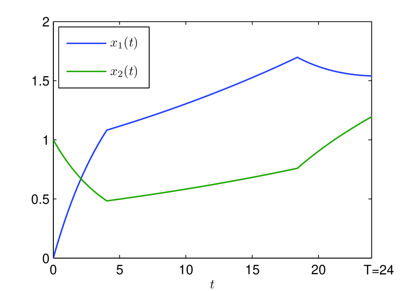
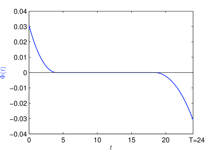
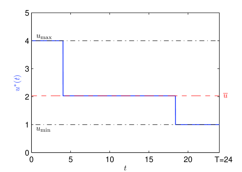
We are now ready to exhibit the unique optimal control when the horizon $T$ is large enough. It consists mainly in the singular control $u_{\mathrm{sing}}$, except in the regions close to the endpoints of $[0,T]$. For small time, the optimal control depends on the initial data $x^{0}$ and it consists in reaching as fast as possible the singular trajectory. Then the control remains constant equal to the value which maximizes the Perron eigenvalue (see Figure 4). At the end of the experiment, the control is $u_{\min}$ due to the transversality condition induced by the objective function. This kind of strategy is known as turnpike properties (see [35, 37] for instance), the “turnpike” is the singular trajectory which corresponds to the Perron eigenvector $X$ with an exponential growth of maximal rate $\lambda_{P}(\bar{u})$.

We divide the construction of the optimal control in two steps. First, we build a control such that the PMP is satisfied (Theorem 17). Then, with an analysis of the switching function $\Phi(t)$, we prove that this is the only possible one (Theorem 18).

Before stating the results, let us define projective variables. For $x=(x_{1},x_{2})^{T}$ and $p=(p_{1},p_{2})$, where $x_{1}$, $x_{2}$, $p_{1}$ and $p_{2}$ are positive real numbers, we define

$$y:=\frac{x_{1}}{x_{1}+x_{2}}\in[0,1]\quad\text{ and }\quad q:=\frac{p_{1}}{p_{1}+p_{2}}\in[0,1].$$

For $(x(t),p(t))$ a solution to (4.2)-(4.3), the projections $y(t)$ and $q(t)$ satisfy the dynamics

$$\dot{y}=\mathcal{Y}(y,u):=2u\beta-(3u\beta+(u\theta+\zeta)\tau)y+u\beta y^{2},$$ (4.20)

$$\dot{q}=\mathcal{Q}(q,u):=-\bigl{[}(\theta u+\zeta)\tau-(3(\theta u+\zeta)\tau-u\beta)q+(2(\theta u+\zeta)\tau-3u\beta)q^{2}\bigr{]}.$$ (4.21)

In our problem the initial condition $x(0)=x^{0}=(x^{0}_{1},x^{0}_{2})^{T}>0$ and the terminal condition $p(T)=\Psi=(1,2)>0$ guarantee that $x(t)$ and $p(t)$ are positive for all $t\in[0,T].$ So $y(t)$ and $q(t),$ which satisfy

$$y(0)=\frac{x_{1}^{0}}{x_{1}^{0}+x_{2}^{0}}\qquad\text{and}\qquad\displaystyle q(T)=\frac{1}{3},$$

are well defined and belong to $(0,1)$ for every time $t\in[0,T].$ Finally for $u$ in $[u_{\text{min}},u_{\text{max}}]$, let $Y(u)\in(0,1)$ be the projection of the Perron eigenvector $X(u)$ of the matrix $uF+(\theta u+\zeta)G$ and let $\pi(u)$ be the projection of the adjoint Perron eigenvector $\phi(u)$.

Theorem 17.

There exist a time $T_{\psi}>0$ and a function $T_{0}$ defined on $[0,1]$, satisfying

$$\forall y\in[0,1]\setminus\{Y(\bar{u})\},\ T_{0}(y)>0,\qquad T_{0}(Y(\bar{u}))=0,\qquad\sup_{[0,1]}T_{0}<+\infty,$$

such that, for $T>T_{0}(y(0))+T_{\psi}$, the control defined by

$$u^{*}(t)=\left\{\begin{array}[]{ll}\left\{\begin{array}[]{l}u_{\min}\ \text{if}\ y(0)>Y(\bar{u})\\ u_{\max}\ \text{if}\ y(0)<Y(\bar{u})\end{array}\right.&\text{for}\ t\in[0,T_{0}(y(0))],\vspace{1mm}\\ \ \bar{u}&\text{for}\ t\in(T_{0}(y(0)),T-T_{\psi}],\\ \ u_{\min}&\text{for}\ t\in(T-T_{\psi},T],\end{array}\right.$$ (4.22)

satisfies the maximality property (4.6). Moreover the corresponding trajectories $y^{*}(t)$ and $q^{*}(t)$ satisfy $y^{*}\equiv Y(\bar{u})$ and $q^{*}\equiv\pi(\bar{u})$ on $[T_{0}(y(0)),T-T_{\psi}]$.

Based on Theorem 17, we can state our main theorem.

Theorem 18.

There exists a time $T_{c}>T_{\psi}+\displaystyle\sup_{[0,1]}T_{0}$ such that, for every final time $T>T_{c}$, the control defined by (4.22) is the unique solution to the optimal relaxed control problem (4.4).

For the optimal relaxed control $(u^{*},\sigma(u^{*}))\to\Sigma$ given by (4.22), we can easily build a sequence of piecewise constant functions $(u^{n},v^{n})_{n\in\mathbb{N}}\to\Omega$ which converges weakly to $(u^{*},\sigma(u^{*})),$ as claimed in (3.9). It suffices to replace $u^{*}=\bar{u}$ on the interval $[T_{0},T-T_{\psi})$ by

$$u^{n}(t)=\left\{\begin{array}[]{ll}u_{\min}&\text{if}\quad t\in[T_{0}+(k-1)\Delta t,T_{0}+(k-1)\Delta t+\Delta_{\min})\vspace{1mm}\\ u_{\max}&\text{if}\quad t\in[T_{0}+(k-1)\Delta t+\Delta_{\min},T_{0}+k\Delta t)\end{array}\right.,\quad\text{for}\quad k=1,\cdots,n,$$

where we have defined

$$\Delta t=\frac{T-(T_{0}+T_{\psi})}{n},\qquad\Delta_{\min}:=\frac{u_{\max}-\bar{u}}{u_{\max}-u_{\min}}\,\Delta t\qquad\text{and}\qquad\Delta_{\max}:=\frac{\bar{u}-u_{\min}}{u_{\max}-u_{\min}}\,\Delta t,$$ (4.23)

and to set $v^{n}=r(u^{n}).$ This sequence oscillates more when $n$ increases, keeping the same mean values

$$\int_{0}^{T}u^{n}(t)\,dt=\int_{0}^{T}u^{*}(t)\,dt\qquad\text{and}\qquad\int_{0}^{T}v^{n}(t)\,dt=\int_{0}^{T}v^{*}(t)\,dt.$$

This is what happens in Figure 1 when we solve numerically a discretized optimal control problem.

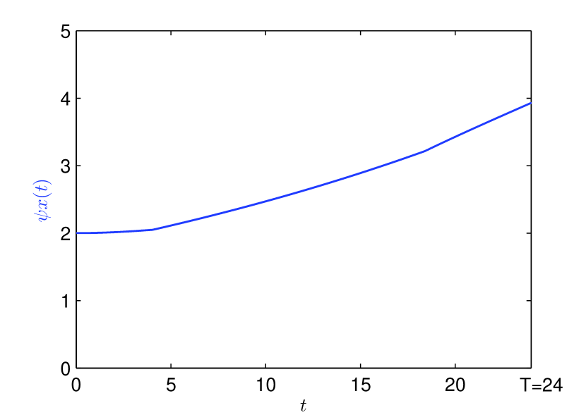
Figure 4: Top left: the optimal control for $T=24,$ $n=2,$ $\theta=-0.2,$ $\zeta=1,$ $\tau=0.1,$ $\beta=0.05$ and the initial data $x^{0}=(0,1)^{T}.$ Top right: the corresponding trajectories $x_{1}(t)$ and $x_{2}(t).$ Bottom left: the switching function $\Phi(t).$ Bottom right: the evolution of the objective $\psi x(t)=x_{1}(t)+2x_{2}(t).$

Before proving Theorems 17 and 18, we give some useful preliminary results. First note that for $u$ fixed in $[u_{\text{min}},u_{\text{max}}],$ $Y(u)$ and $\pi(u)$ are the unique steady states of respectively (4.20) and (4.21) in the interval $[0,1].$ Moreover we know the sign of the vector fields.

Lemma 19.

For every $u$ in $[u_{\text{min}},u_{\text{max}}]$,

$$(y-Y(u))\mathcal{Y}(y,u) <0,\qquad\forall y\in[0,1]\setminus\{Y(u)\},$$ (4.24)

$$(q-\pi(u))\mathcal{Q}(q,u) >0,\qquad\forall q\in[0,1]\setminus\{\pi(u)\}.$$ (4.25)

Proof.

Let $u\in[u_{\text{min}},u_{\text{max}}].$ The function $y\mapsto(y-Y(u))\mathcal{Y}(y,u)$ is a third order polynomial which vanishes only at $y=Y(u)$ on the interval $[0,1].$ We obtain (4.24) by computing for instance $\mathcal{Y}(0,u)=2u\beta>0$ and $\mathcal{Y}(1,u)=-(u\theta+\zeta)\tau<0.$ The same argument allows to prove (4.25). ∎

Corollary 20.

For $u$ fixed in $[u_{\text{min}},u_{\text{max}}]$, every solution $y$ of (4.20) with $y(0)$ in $[0,1]$ satisfies

$$(y(t)-Y(u))^{2}\downarrow 0\quad\text{when}\quad t\to+\infty,$$

and every solution $q$ of (4.21) with $q(0)$ in $[0,1]$ satisfies

$$(q(t)-\pi(u))^{2}\downarrow 0\quad\text{when}\quad t\to-\infty.$$

Proof.

We get from (4.24) that

$$\frac{d}{dt}(y(t)-Y(u))^{2}=2(y(t)-Y(u))\mathcal{Y}(y(t),u)<0$$

while $y(t)\neq Y(u),$ and from (4.25) that

$$\frac{d}{dt}(q(-t)-\pi(u))^{2}=-2(q(-t)-\pi(u))\mathcal{Q}(q(-t),u)<0$$

while $q(t)\neq\pi(u).$ ∎

Remark 21.

Corollary 20 allows to recover the property that $y(t)\in(0,1)$ and $q(t)\in(0,1)$ for every $t\in[0,T]$ as soon as $y(0)\in(0,1)$ and $q(T)\in(0,1).$

From the proof of Corollary 20 we readily get another useful consequence of Lemma 19.

Corollary 22.

For $u$ fixed in $[u_{\text{min}},u_{\text{max}}],$ every solution $y$ of (4.20) satisfies

$$\left\{\begin{array}[]{l}0<y(0)<Y(u)\implies\exists!\,T>0,\ y(-T)=0,\vspace{2mm}\\ Y(u)<y(0)<1\implies\exists!\,T>0,\ y(-T)=1.\end{array}\right.$$

The following lemma orders the steady states $Y(u)$ and $\pi(u)$ for different values of $u.$

Lemma 23.

We have the comparisons

$$Y(u_{\text{min}})<Y(\bar{u})<Y(u_{\text{max}})\qquad\text{and}\qquad\pi(u_{\text{min}})>\pi(\bar{u})>\pi(u_{\text{max}})>\frac{1}{3}.$$

Proof.

We study the variations of the function $u\mapsto Y(u)$. Starting from the computations in the computational proof of Theorem 14 in Appendix C, we get

$$Y(u)=\frac{\lambda_{P}(u)+u\beta}{\lambda_{P}(u)+u\beta+(u\theta+\zeta)\tau}=\frac{u\beta-(u\theta+\zeta)\tau+\sqrt{\Delta}}{u\beta+(u\theta+\zeta)\tau+\sqrt{\Delta}},$$

and by differentiation

$$Y^{\prime}(u)=\frac{2h(u)}{\bigl{(}u\beta+(u\theta+\zeta)\tau+\sqrt{\Delta}\bigr{)}^{2}}\qquad\text{with}\qquad h(u):=\beta\zeta\tau-\theta\tau\sqrt{\Delta}+\frac{\Delta^{\prime}}{2\sqrt{\Delta}}(u\theta+\zeta)\tau.$$

To have the sign of $h$ on $[0,\displaystyle\frac{\zeta}{-\theta}]$, we differentiate $h$ with respect to $u$

$$h^{\prime}(u)=\frac{(u\theta+\zeta)\tau}{4\Delta\sqrt{\Delta}}\left(2\Delta\Delta^{\prime\prime}-(\Delta^{\prime})^{2}\right).$$

We know from Lemma 33 in Appendix C that $2\Delta\Delta^{\prime\prime}-(\Delta^{\prime})^{2}<0.$ So $h$ is decreasing and since $h(\displaystyle\frac{\zeta}{-\theta})=2\zeta\beta\tau>0$, we get that $h>0$ on $[0,\displaystyle\frac{\zeta}{-\theta}]$. Then $Y$ is increasing and

$$Y(u_{\min})<Y(\bar{u})<Y(u_{\max}).$$

For the variations of $\pi(u),$ we compute

$$\pi(u)=\frac{\lambda_{P}(u)+u\beta}{\lambda_{P}(u)+3u\beta}=\frac{u\beta-(u\theta+\zeta)\tau+\sqrt{\Delta}}{5u\beta-(u\theta+\zeta)\tau+\sqrt{\Delta}}$$

and

$$\pi^{\prime}(u)=\frac{4g(u)}{\left(5u\beta-(u\theta+\zeta)\tau+\sqrt{\Delta}\right)^{2}}\qquad\text{with}\qquad g(u)=\beta\left(\zeta\tau-\sqrt{\Delta}+\frac{u\Delta^{\prime}}{2\sqrt{\Delta}}\right).$$

Using Lemma 33 in Appendix C we have

$$g^{\prime}(u)=\frac{\beta}{4\Delta\sqrt{\Delta}}\left(2\Delta\Delta^{\prime\prime}-(\Delta^{\prime})^{2}\right)<0,$$

so $g<0$ since $g(0)=0$. We obtain that $\pi(u)$ is decreasing and

$$\pi(u_{\min})>\pi(\bar{u})>\pi(u_{\max})>\pi\Bigl{(}\frac{\zeta}{-\theta}\Bigr{)}=\frac{1}{3}.$$

∎

We give now a last lemma and a corollary, which are key points in the proofs of Theorem 17 and Theorem 18.

Lemma 24.

The switching function $\Phi$ defined in (4.5) satisfies the equation

$$\dot{\Phi}=\Lambda_{1}\Phi+\Lambda_{2},$$

with

$$\Lambda_{1}:=\zeta\tau\frac{x_{1}}{x_{2}}\qquad\text{and}\qquad\Lambda_{2}:=\zeta\tau(p_{2}-p_{1})\Bigl{(}-\theta\tau\Bigl{(}\frac{x_{1}}{x_{2}}\Bigr{)}^{2}-2\beta\Bigr{)}x_{2}.$$

Moreover for every $t\in[0,T]$ we have $\Lambda_{1}(t)>0$ and

$$\text{sign}(\Lambda_{2}(t))=\text{sign}(y(t)-Y(\bar{u})),$$

where, for every real number $a$, $\text{sign}(a)=1$ if $a>0$, $\text{sign}(a)=-1$ if $a<0$ and $\text{sign}(a)=0$ if $a=0$.

Proof.

From the positivity of $x(t),$ we get $\Lambda_{1}(t)>0.$ For $\Lambda_{2}$, it is noteworthy from Lemma 10 that $p_{2}-p_{1}>0$. Thus, the sign of $\Lambda_{2}$ does not depend on $p$ and from Corollary 16, we get

$$\text{sign}(\Lambda_{2})=\text{sign}\left(\frac{x_{1}^{2}}{x_{2}^{2}}-\frac{2\beta}{-\theta\tau}\right)=\text{sign}\left(\biggl{(}\frac{y}{1-y}\biggr{)}^{2}-\biggl{(}\frac{Y(\bar{u})}{1-Y(\bar{u})}\biggr{)}^{2}\right)=\text{sign}(y-Y(\bar{u})).$$

∎

Corollary 25.

For all $t>0,$ we have

$$\left\{\begin{array}[]{l}\Bigl{(}\Phi^{*}(t)\geq 0\quad\text{and}\quad y^{*}(t)<Y(\bar{u})\Bigr{)}\implies\Bigl{(}\Phi^{*}(s)>0,\quad\forall s<t\Bigr{)},\vspace{2mm}\\ \Bigl{(}\Phi^{*}(t)\leq 0\quad\text{and}\quad y^{*}(t)>Y(\bar{u})\Bigr{)}\implies\Bigl{(}\Phi^{*}(s)<0,\quad\forall s<t\Bigr{)}.\end{array}\right.$$

Proof.

Assume that $\Phi^{*}(t)\geq 0$ and $y^{*}(t)<Y(\bar{u}).$ If $\Phi^{*}(t)=0,$ then Lemma 24 gives $\dot{\Phi}^{*}(t)<0$ so there exists $t^{\prime}<t$ such that $\Phi^{*}>0$ on $(t^{\prime},t).$ As a consequence $u^{*}\equiv u_{\max}$ on $(t^{\prime},t)$ which ensures by using Lemma 19 and Lemma 23 that $y^{*}(t^{\prime})<Y(\bar{u}).$ So we can restrict to the case $\Phi^{*}(t)>0,\ y^{*}(t)<Y(\bar{u})$ and we suppose by contradiction that

$$\exists t_{0}<t,\ \Phi^{*}(t_{0})=0\ \text{and}\ \Phi^{*}(s)>0,\ \forall s\in(t_{0},t).$$ (4.26)

Using Lemma 19 and Lemma 23, we obtain that $y^{*}<Y(\bar{u})$ on $[t_{0},t].$ By Lemma 24 we get that $\Lambda_{2}<0$ and then $\dot{\Phi}^{*}<\Lambda_{1}\Phi^{*}$ on $[t_{0},t].$ By Grönwall’s inequality we deduce that $\Phi^{*}(t_{0})>\Phi^{*}(t)\,e^{-\int_{t_{0}}^{t}\Lambda_{1}(s)\,ds}>0.$ This contradicts (4.26) so the first implication of Lemma 25 is proved. The proof of the second implication follows from a similar argument. ∎

In the proofs of Theorem 17 and Theorem 18, we will use the following compact definitions: a triplet $(y,u,y^{0})$ (resp. $(q,u,q^{0})$) is said to be solution to (4.20) (resp. to (4.21)) if $y$ satisfies Equation (4.20) (resp. Equation (4.21)) with the control $u$ and the initial condition $y(0)=y^{0}$ (resp. $q(0)=q^{0}).$

Proof of Theorem 17.

We first define $T_{0}.$ From Corollary 20 and Lemma 23, we know that

$$\forall y^{0}\in[0,Y(\bar{u})),\ \exists!\,T_{0}(y^{0})>0,\quad(y,u_{\text{max}},y^{0})\ \text{is solution to \eqref{doty=}}\implies y(T_{0}(y^{0}))=Y(\bar{u}),$$

and

$$\forall y^{0}\in(Y(\bar{u}),1],\ \exists!\,T_{0}(y^{0})>0,\quad(y,u_{\text{min}},y^{0})\ \text{is solution to \eqref{doty=}}\implies y(T_{0}(y^{0}))=Y(\bar{u}).$$

The function $T_{0}$ thus defined is bounded on $[0,1].$ This is a consequence of the Cauchy-Lipschitz theorem for Equation (4.20), which ensures that for all $y\in[0,1],$ $T_{0}(y)\leq\max\{T_{0}(0),T_{0}(1)\}.$

The time $T_{\psi}$ is also defined by using Corollary 20 and Lemma 23

$$\exists!\,T_{\psi}>0,\quad(q,u_{\text{min}},1/3)\ \text{is solution to \eqref{dotq=}}\implies q(-T_{\psi})=\pi(\bar{u}).$$ (4.27)

Once $T_{0}$ and $T_{\psi}$ are defined, it only remains to verify that the control defined by (4.22) and the associated trajectories $y^{*}$ and $q^{*}$ satisfy the maximality condition (4.6). For this, it suffices to check that property (4.7) of the switching function $\Phi^{*}(t)=\Phi(x^{*}(t),p^{*}(t))$ holds (see Figure 4 for a numerical illustration).

In the interval $[T_{0}(y(0)),T-T_{\psi}]$, we have $u^{*}=\bar{u}$, $y^{*}\equiv Y(\bar{u})$ and $q^{*}\equiv\pi(\bar{u})$. Thus, by Theorem 13 and Theorem 14, we have $\Phi^{*}=0$.

We have from the definition of $T_{0}$ that, if $y(0)>Y(\bar{u}),$ then $u^{*}\equiv u_{\min}$ and $y^{*}>Y(\bar{u})$ in the interval $[0,T_{0}(y(0)))$. Using Lemma 24 we deduce from $y^{*}>Y(\bar{u})$ that $\Lambda_{2}>0$ and then, since $\Phi(T_{0}(y(0)))=0$, that $\Phi^{*}<0$ in the interval $[0,T_{0}(y(0)))$. The same argument proves that, if $y(0)<Y(\bar{u})$, then $u^{*}\equiv u_{\max}$ and $\Phi^{*}>0$ in the interval $[0,T_{0}(y(0)))$.

In the interval $(T-T_{\psi},T]$ we have $u^{*}(t)\equiv u_{\min},$ so we get from $y^{*}(T-T_{\psi})=Y(\bar{u}),$ Corollary 20 and Lemma 23 that $y^{*}(t)<Y(\bar{u})$. It follows from Lemma 24 that for every $t\in(T-T_{\psi},T],$ $\Lambda_{2}(t)<0$, and then $\Phi^{*}(t)<0$ since $\Phi^{*}(T-T_{\psi})=0$.

∎

Proof of Theorem 18.

Let $t\in[0,T]\mapsto u^{*}(t)$ be a control such that the maximality condition (4.6) is satisfied. Let $x^{*}$, $p^{*}$, $y^{*}$, $q^{*}$ and $\Phi^{*}$ be the corresponding functions. Since $\Phi^{*}(T)=\theta\tau x_{1}^{*}(T)<0$, necessarily, $u^{*}=u_{\min}$ in a neighborhood of $T$. We start from time $T$ and analyze the problem backward in time.

First step: we prove by contradiction that

$$\exists\eta,T_{1}>0\ \text{(both independent of $x^{0}$) s.t.}\quad T>T_{1}\implies y^{*}(T)\not\in[Y(u_{\min})-\eta,Y(u_{\min})+\eta].$$

We start from the fact that

$$\phi(u_{\min})(F+\theta G)X(u_{\min})=\lambda_{P}^{\prime}(u_{\min})>0.$$ (4.28)

(The first equality of (4.28) can be obtained by differentiating $(u(F+\theta G)+\zeta G)X(u)=\lambda_{P}(u)X(u)$ with respect to $u$ and by using $\phi(u)(u(F+\theta G)+\zeta G)=\lambda_{P}(u)\phi(u)$.) Property (4.28) ensures that there exists $\varepsilon>0$ such that

$$\max\{|y-Y(u_{\min})|,|q-\pi(u_{\min})|\}\leq\varepsilon\quad\Longrightarrow\quad\Phi(x,p)>0.$$ (4.29)

Using Lemma 23 and decreasing $\varepsilon>0$ if necessary, we may assume that $\pi(u_{\min})-\varepsilon>1/3$. Then from Corollary 20 and Lemma 23 we have that

$$\exists!\,T_{1,1}>0,\quad(q,u_{\text{min}},1/3)\ \text{is solution to \eqref{dotq=}}\implies q(-T_{1,1})=\pi(u_{\min})-\varepsilon.$$

Consider now $\eta>0$ such that, for $(y,u_{\min},y^{0})$ solution to (4.20),

$$y^{0}\in[Y(u_{\min})-\eta,Y(u_{\min})+\eta]\implies\forall t\in[-T_{1,1},0],\ y(t)\in[Y(u_{\min})-\varepsilon,Y(u_{\min})+\varepsilon].$$ (4.30)

(This $\eta>0$ exists since $(y,u):=(Y(u_{\min}),u_{\min})$ is a solution of (4.20).) Still decreasing $\varepsilon>0$ if necessary and using Lemma 23, we may assume that

$$Y(u_{\min})+\varepsilon<Y(\bar{u}).$$ (4.31)

By Corollary 22, Lemma 23 and (4.31)

$$\exists!\,T_{1,2}>0,\quad(y,u_{\max},Y(u_{\min})+\varepsilon)\ \text{is solution to \eqref{doty=}}\implies y(-T_{1,2})=0.$$

Let $T_{1}:=T_{1,1}+T_{1,2}$ and $T>T_{1}$. Let us assume that $y^{*}(T)$ belongs to $[Y(u_{\min})-\eta,Y(u_{\min})+\eta]$. If $\Phi^{*}<0$ in $[T-T_{1,1},T]$, then $u^{*}\equiv u_{\min}$ in $[T-T_{1,1},T]$, and, by the definition (4.30) of $\eta$, $y^{*}(T-T_{1,1})\in[Y(u_{\min})-\varepsilon,Y(u_{\min})+\varepsilon]$, which, together with (4.29) gives $\Phi^{*}(T-T_{1,1})>0$. Hence $\Phi^{*}<0$ on $[T-T_{1,1},T]$ does not hold and there exists $t_{0}\in[T-T_{1,1},T]$ such that $\Phi^{*}(t_{0})=0$ and $\Phi^{*}<0$ in $(t_{0},T]$. From (4.30) we have $y^{*}(t_{0})\leqslant Y(u_{\min})+\varepsilon<Y(\bar{u})$, which, with Corollary 25, gives that $\Phi^{*}(t)>0$ for every $t\in[0,t_{0}).$ In particular, $u^{*}\equiv u_{\max}$ on $[0,t_{0}]$. Finally, using the definition of $T_{1,2}>0$, we get that $y^{*}(T-t_{0}-T_{1,2})\leqslant 0$, which is not possible since $x^{*}>0$ in $[0,T]$. So $y^{*}(T)$ cannot belong to $[Y(u_{\min})-\eta,Y(u_{\min})+\eta]$.

Second step: we prove that

$$\exists T_{2}>0,\qquad T>T_{2}\implies y^{*}(T)\not\in[0,Y(u_{\min})-\eta].$$

By Corollary 22,

$$\exists!\,T_{2,1}>0,\quad(y,u_{\min},Y(u_{\min})-\eta)\ \text{is solution to \eqref{doty=}}\implies y(-T_{2,1})=0$$

and, using additionally Lemma 23,

$$\exists!\,T_{2,2}>0,\quad(y,u_{\max},Y(u_{\min})-\eta)\ \text{is solution to \eqref{doty=}}\implies y(-T_{2,2})=0.$$

For $T>T_{2}:=T_{2,1}+T_{2,2}$, the terminal value $y^{*}(T)$ cannot belong to $[0,Y(u_{\min})-\eta]$. If $y^{*}(T)$ is in $[0,Y(u_{\min})-\eta]$, then either $\Phi^{*}(t)<0$ on $[T-T_{2,1},T]$ and in this case $y^{*}(T-T_{2,1})\leq 0,$ or there exists $t_{0}\in[T-T_{2,1},T]$ such that $\Phi^{*}(t_{0})=0$ and in this case we have from Corollary 25 that $\Phi^{*}(t)>0$ for $t<t_{0}$, so $u=u_{\max}$ and $y^{*}(t_{0}-T_{2,2})\leq 0.$ Neither of these two cases is possible since $x^{*}>0$ on $[0,T]$.

Third step: we prove that

$$\exists T_{3}>0,\qquad T>T_{3}\implies y^{*}(T)\not\in[Y(u_{\min})+\eta,1]\setminus\{Y_{\psi}\}$$

where $Y_{\psi}:=y(T_{\psi})$ for $(y,u_{\min},Y(\bar{u}))$ solution to (4.20), with $T_{\psi}$ defined in (4.27).

We start from the fact that, by Corollary 22,

$$\exists!\,T_{3,1}>0,\qquad(y,u_{\min},Y(u_{\min})+\eta)\ \text{is solution of \eqref{doty=}}\implies y(-T_{3,1})=1.$$

Let us assume that $T>T_{3,1}$. If $y^{*}(T)\in(Y(u_{\min})+\eta,1]$, then there exists a time $t_{0}>T-T_{3,1}$ such that $\Phi^{*}(t_{0})=0$ because $y^{*}(t)$ has to be less than $1$ for every time in $[0,T]$. Increasing $t_{0}$ if necessary, we may also impose that $\Phi^{*}<0$ in $(t_{0},T]$. It is not possible to have $y^{*}(t_{0})>Y(\bar{u})$ because in this case, by Lemma 24, we would have $\Phi^{*}(t_{0})=0$ with $(\Phi^{*})^{\prime}(t_{0})=\Lambda_{2}(t_{0})>0$, which cannot hold since $\Phi^{*}<0$ in $(t_{0},T]$. So we necessarily have $y^{*}(t_{0})\leq Y(\bar{u})$.

If $y^{*}(t_{0})<Y(\bar{u})$, then, by Corollary 25, $\Phi^{*}$ is positive on $[0,t_{0}).$ But by Corollary 22 and Lemma 23

$$\exists!\,T_{3,2}>0,\qquad(y,u_{\max},Y(\bar{u}))\ \text{is solution of \eqref{doty=}}\implies y(-T_{3,2})=0.$$

So we get that $y^{*}(t_{0})$ cannot be less than $Y(\bar{u})$ if $T>T_{3}:=T_{3,1}+T_{3,2}$.

Hence, for $T>T_{3}$, we have $y^{*}(t_{0})=Y(\bar{u})$. We deduce from this identity, together with $\Phi^{*}(t_{0})=0$, that $q^{*}(t_{0})=\pi(\bar{u})$ and it implies that $t_{0}=T-T_{\psi}$, where $T_{\psi}$ is defined in the proof of Lemma 17. As a consequence, the only possible value for $y^{*}(T)$ is $Y_{\psi}=y(T_{\psi})\in(Y(\bar{u}),1)$, where $y$ is the solution of (4.20) with $u\equiv u_{\min}$ such that $y(0)=Y(\bar{u})$.

Here, we have proved that, for $T>\max\{T_{1},T_{2},T_{3}\}$, the only possible control which satisfies the PMP takes the value $u_{\min}$ in $[T-T_{\psi},T]$. Moreover, the associated trajectories satisfy $y^{*}(T-T_{\psi})=Y(\bar{u})$ and $q^{*}(T-T_{\psi})=\pi(\bar{u})$. Then, using Lemma 19 and Corollary 25 with the same kind of arguments as above, it is straightforward to check that the control defined by (4.22) is the only control which satisfies the PMP for $T>T_{c}:=\max\{T_{1},T_{2},T_{3}\}$. Since any optimal control satisfies the maximality condition (4.6), we conclude that this is the only optimal control.

∎

Corollary 26.

Asymptotically in $T$ we have the convergence

$$\lim_{T\to+\infty}\frac{\ln(J(u^{*}))}{T}=\lambda_{P}(\bar{u}).$$

A similar ergodic result is proved in [4] in the case of dimension $n=3$ but without proving that the limit is $\lambda_{P}(\bar{u})$.

5 Conclusion and perspectives

We have modeled the PMCA protocol by a system of differential equations with a control term. The analysis of the optimal control problem, which aims to maximize the efficiency of the PMCA, makes appear that the solution may not be a classical control but a relaxed one. Such a theoretical optimal control cannot be realized experimentally. Nevertheless it can be approached by altering incubation and sonication phases.

Our main result provides, in dimension 2, the optimal ratio between the two phases. It is given by $R_{\text{opt}}:=\frac{\Delta_{\max}}{\Delta_{\min}}=\frac{\bar{u}-u_{\min}}{u_{\max}-\bar{u}}$ (see (4.23)), where $\bar{u}\in(u_{\min},u_{\max})$ is the constant which maximizes the Perron eigenvalue in the convex hull of the original control set. To approach the optimal relaxed control via an alternation of incubation and sonication phases, the switching frequency has to be high. But the frequency is limited experimentally, for instance due to the warming engendered by the sonication. To maintain the temperature of the sample at a reasonable level, sufficiently long rest phases (corresponding to incubation) have to be intercalated between the sonication phases. Considering such experimental constraints, a close-to-optimal strategy should be to switch as fast as possible between sonication and incubation phases, keeping the optimal ratio $R_{\text{opt}}$ between the respective durations.

Before practicing this strategy in a real PMCA protocol, the parameters of the model have to be estimated from experiments. This requires precise measurements of the size distribution of the polymers and inverse problem methods as the one detailed in [11] (see also the references therein). To use our result in dimension 2, the sizes of the polymers have to be divided into two pools and the mean polymerization and fragmentation coefficients of the two pools have to be estimated. If one wants to improve the accuracy of the method, a higher dimensional model should be used. But it appears that, even for the case of three compartments, the mathematical analysis is much more delicate than in dimension two.

Appendix

Appendix A Perron eigenvalue

For $u>0$ fixed and $r(u)>0,$ denote by $(\lambda_{P}(u),X_{P}(u),\phi_{P}(u))$ the Perron eigenelements of the matrix $M(u):=uF+r(u)G$ defined by

$$\left\{\begin{array}[]{lll}\lambda_{P}X_{P}=M(u)X_{P},&\quad X_{P}>0,&\quad\|X_{P}\|_{1}=1,\\ \lambda_{P}\phi_{P}=\phi_{P}M(u),&\quad\phi_{P}>0,&\quad\phi_{P}X_{P}=1.\end{array}\right.$$

In the current section we investigate the dependence of these elements on the control parameter $u.$ Such eigenelements also exist for the continuous growth-fragmentation equation (1.1) (see [9] for instance), and their dependence on parameters is investigated in [3, 13].

The function $r:\mathbb{R}^{+}\to\mathbb{R}^{+*}$ is assumed to be continuous and bounded. Theorem 1 is an immediate consequence of the following Lemma 27 and Theorem 28.

Lemma 27.

The eigenelements $\lambda_{P}$, $X_{P}$ and $\phi_{P}$ are continuous functions of $u$ on $\mathbb{R}^{+}$. Moreover, we have

$$\lambda_{P}(u)>0\ \text{for}\ u>0\qquad\text{and}\qquad\lim_{u\to 0}\lambda_{P}(u)=0.$$

Proof.

Since the function $r$ is continuous, the coefficients of the matrix $M(u)$ depend continuously on $u$. As a consequence, the characteristic polynomial of $M(u)$ varies continuously with $u$. The first eigenvalue $\lambda_{P}$ is the largest root of this characteristic polynomial and the Perron-Frobenius theorem ensures that the multiplicity of this root is 1. So $\lambda_{P}$ is a continuous function of $u$.

Let $u\geq 0$ and $(u_{k})_{k\in\mathbb{N}}$ be a positive sequence which converges to $u$. Since $\|X_{P}(u_{k})\|_{1}=1$ there exists a subsequence of $(X_{P}(u_{k}))_{k}$ which converges to a limit $X_{\infty}$. By continuity of $\lambda_{P}(u)$ and $M(u)$, this limit satisfies $M(u)X_{\infty}=\lambda_{P}(u)X_{\infty}$ and $\|X_{\infty}\|_{1}=1$. By uniqueness of the first eigenvector, we conclude that the whole sequence $(X_{P}(u_{k}))_{k}$ converges to $X_{\infty}=X_{P}(u)$ and so $X_{P}$ is a continuous function of $u$. Since $(X_{P}(u_{k}))_{k}$ is a positive convergent sequence, it is lower bounded and we deduce from the normalization $\phi_{P}X_{P}=1$ that the sequence $(\phi_{P}(u_{k}))_{k}$ is bounded. The same as for $X_{P}$, we conclude from the uniqueness of the adjoint eigenvector that $\phi_{P}$ is a continuous function of $u$.

Define $\Theta:=(1,1,\cdots,1)$ and, for $j=2,\cdots,n,$ $K_{j}:=\sum_{i=1}^{j-1}\kappa_{ij}>0.$ We have: $\Theta X_{P}=\|X_{P}\|_{1}=1$ since $X_{P}>0,$ $\Theta G=0$ from (1.5), and $\Theta F=(0,K_{2}\beta_{2},\cdots,K_{n}\beta_{n})^{T}$ from (1.11). So multiplying the identity $\lambda_{P}X_{P}=M(u)X_{P}$ by $\Theta$ we get

$$\lambda_{P}(u)=u\,\Theta FX_{P}\leq u\,\max_{2\leq j\leq n}K_{j}\beta_{j}$$

which ensures that $\lambda_{P}(u)$ is positive for $u$ positive and tends to zero when $u\to 0$.

∎

Theorem 28.

Under Assumptions (2.1) and (2.2), we have the expansions

$$\begin{array}[]{l}\displaystyle k<l,\quad\implies\quad\lambda_{P}(u)=r_{0}\tau_{1}+\left[r_{0}^{k+1}(\tau_{k+1}-(k+1)\tau_{1})\prod_{i=1}^{k}\frac{\tau_{i}}{\beta_{i+1}}\right]u^{-k}+\underset{u\to+\infty}{o}(u^{-k}),\\ \displaystyle k=l,\quad\implies\quad\lambda_{P}(u)=r_{0}\tau_{1}+\left[r_{0}^{k+1}(\tau_{k+1}-(k+1)\tau_{1})\prod_{i=1}^{k}\frac{\tau_{i}}{\beta_{i+1}}+r_{k}\tau_{1}\right]u^{-k}+\underset{u\to+\infty}{o}(u^{-k}),\vspace{.4cm}\\ \displaystyle k>l,\quad\implies\quad\lambda_{P}(u)=r_{0}\tau_{1}+r_{l}\tau_{1}u^{-l}+\underset{u\to+\infty}{o}(u^{-l}).\end{array}$$

This result can be related to Corollary 1 in [3] which provides an expansion of the first eigenvalue for the continuous growth-fragmentation model. The proof of Theorem 28 uses the following lemma which gives the asymptotic behavior of the eigenvector $X_{P}=(x_{1},x_{2},\cdots,x_{n})^{T}$.

Lemma 29.

Assume that $r(u)$ admits a limit $r_{0}>0$ when $u$ tends to $+\infty$, then

$$\forall i\in[1,n],\qquad x_{i}(u)\underset{u\to+\infty}{\sim}r_{0}^{i-1}\prod_{j=1}^{i-1}\frac{\tau_{j}}{\beta_{j+1}}\,u^{1-i}.$$ (A.1)

Proof of Lemma 29.

We prove by induction on $i$ that

$$u^{i-1}x_{i}(u)\xrightarrow[u\to+\infty]{}r_{0}^{i-1}\prod_{j=1}^{i-1}\frac{\tau_{j}}{\beta_{j+1}}\qquad\text{and}\quad u^{i-1}x_{j}(u)\xrightarrow[u\to+\infty]{}0,\qquad\forall j>i.$$ (IH)

$i=1:$ We have by definition

$$(r(u)G+uF)X_{P}(u)=\lambda_{P}(u)X_{P}(u)\qquad\text{with}\quad\|X_{P}(u)\|_{1}=1.$$ (A.2)

We use $\psi=(1,2,\cdots,n)$, which satisfies $\psi F=0$ (see (3.6)). Testing (A.2) against $\psi$ on the left, we obtain

$$r(u)\psi GX_{P}(u)=\lambda_{P}(u)\psi X_{P}(u)$$ (A.3)

and so $\lambda_{P}(u)$ is bounded since $\|X_{P}(u)\|_{1}=1$ and $r$ is bounded. Dividing by $u$ in (A.2), we get

$$\left(\frac{r(u)}{u}G+F\right)X_{P}(u)=\frac{\lambda_{P}(u)}{u}X_{P}(u).$$ (A.4)

The sequence $X_{P}(u)$ is bounded and thus convergence occurs when $u\to+\infty$ for a subsequence. But from (A.4) the limit $X_{P}^{\infty}$ must satisfy $FX_{P}^{\infty}=0$ so the whole sequence converges to

$$X_{P}^{\infty}=\delta:=(1,0\,\cdots,0)^{T}.$$

$i\to i+1:$ ($i+1\leq n$) We have

$$u^{i}FX_{P}(u)=u^{i-1}\lambda_{P}(u)X_{P}(u)-u^{i-1}r(u)GX_{P}(u).$$

We consider the $n-i$ last lines of this matrix identity and find

$$\left(\begin{array}[]{ccc}-\beta_{i+1}&&\\ &&(2\kappa_{kj}\beta_{j})\\ &\ddots&\\ \text{\Large$0$}&&\\ &&-\beta_{n}\end{array}\right)\left(\begin{array}[]{c}u^{i}x_{i+1}(u)\\ \\ \vdots\\ \\ u^{i}x_{n}(u)\end{array}\right) =\left(\begin{array}[]{c}(\lambda_{P}(u)+r(u)\tau_{i+1})u^{i-1}x_{i+1}(u)-r(u)\tau_{i}u^{i-1}x_{i}(u)\\ \\ \vdots\\ \\ \lambda_{P}(u)u^{i-1}x_{n}(u)-r(u)\tau_{n-1}u^{i-1}x_{n-1}(u)\end{array}\right)$$

$$\xrightarrow[u\to+\infty]{\text{by~{}\eqref{eq:IH}}}\left(\begin{array}[]{c}\displaystyle-r_{0}\tau_{i}\cdot r_{0}^{i-1}\prod_{j=1}^{i-1}\frac{\tau_{j}}{\beta_{j+1}}\\ \\ \text{\Large$0$}\\ \\ \end{array}\right),$$

which concludes the proof of Lemma 29. ∎

Proof of Theorem 28.

Notice that $k<n$ since $\tau_{n}=0$ and $\tau_{1}>0$. Using (A.3), the convergence of $X_{P}$ to $\delta=(1,0\,\cdots,0)^{T}$ and the convergence of $r$ to $r_{0},$ we obtain that $\lambda_{P}(u)$ converges when $u\to+\infty$ and that the limit $\lambda_{P}^{\infty}$ satisfies

$$r_{0}\psi G\delta=\lambda_{P}^{\infty}\psi\delta,$$ (A.5)

which gives

$$\lambda_{P}^{\infty}=r_{0}\tau_{1}.$$ (A.6)

Once we have this limit, we need to estimate the difference $\lambda_{P}(u)-\lambda_{P}^{\infty}$ when $u\to+\infty.$ To do so we make the difference between (A.3) and (A.5) which gives, by using (A.6),

$$(\lambda_{P}(u)-r_{0}\tau_{1})\psi X_{P}(u)+r_{0}\tau_{1}\psi(X_{P}(u)-\delta)=r(u)\psi G(X_{P}(u)-\delta)+(r(u)-r_{0})\psi G\delta.$$ (A.7)

Now we use the result of Lemma 29 which gives an equivalent to $X_{P}(u)$ when $u\to+\infty,$ and Assumption (2.1) which gives an equivalent to $r(u)-r_{0}$ when $u\to+\infty,$ to deduce an equivalent to $\lambda_{P}(u)-\lambda_{P}^{\infty}.$ Denoting $m:=\min{(k,l)}$, we obtain from (A.7)

$$u^{m}(\lambda_{P}(u)-r_{0}\tau_{1})\psi X_{P}(u) =u^{m}r(u)\psi G(X_{P}(u)-\delta)+u^{m}(r(u)-r_{0})\psi G\delta-u^{m}r_{0}\tau_{1}\psi(X_{P}(u)-\delta)$$

$$=u^{m}r_{0}\psi(G-\tau_{1}Id)(X_{P}(u)-\delta)+u^{m}(r(u)-r_{0})\psi GX_{P}(u)$$

$$=u^{m}r_{0}\sum_{j=1}^{n-1}(\tau_{j}-j\tau_{1})(x_{j}(u)-\delta_{1,j})+u^{m}(r(u)-r_{0})\psi GX_{P}(u)$$

$$=r_{0}\sum_{j=k+1}^{n-1}(\tau_{j}-j\tau_{1})u^{m}x_{j}(u)+u^{m}(r(u)-r_{0})\psi GX_{P}(u)$$

$$\xrightarrow[u\to+\infty]{\eqref{eq:expeigenvector}}{\mathchoice{\rm 1\mskip-4.0mul}{\rm 1\mskip-4.0mul}{\rm 1\mskip-4.5mul}{\rm 1\mskip-5.0mul}}_{\{k\leq l\}}r_{0}^{k+1}(\tau_{k+1}-(k+1)\tau_{1})\prod_{i=1}^{k}\frac{\tau_{i}}{\beta_{i+1}}+{\mathchoice{\rm 1\mskip-4.0mul}{\rm 1\mskip-4.0mul}{\rm 1\mskip-4.5mul}{\rm 1\mskip-5.0mul}}_{\{k\geq l\}}r_{l}\tau_{1},$$

where $\delta_{1,j}=1$ if $j=1$ and $\delta_{1,j}=0$ otherwise. ∎

Appendix B Floquet eigenvalue

For a $T$-periodic control $u(t)$, the Floquet theorem ensures that there is a Floquet eigenvalue $\lambda_{F}[u(\cdot)]$ and a $T$-periodic function $X_{F}[u(\cdot)](t)$ solution to

$$\frac{d}{dt}X_{F}(t)=[M(u(t))-\lambda_{F}]X_{F}(t).$$

The Floquet eigenvalues can sometimes be compared to the Perron eigenvalues [8, 14]. Here we make periodic variations around the optimal constant control $u_{\mathrm{opt}}$ to find whether or not periodic controls can provide a better eigenvalue than $\lambda_{P}(u_{\mathrm{opt}}).$

Consider directional perturbations $u(t)=u_{\mathrm{opt}}+\varepsilon\gamma(t)$, where $\gamma$ is a fixed $T$-periodic function and $\varepsilon$ a varying parameter. For the sake of clarity, we denote by $\lambda_{F}(\varepsilon):=\lambda_{F}[u_{\mathrm{opt}}+\varepsilon\gamma(\cdot)]$ the Floquet eigenvalue associated to $\varepsilon$, $X_{F}(\varepsilon;t):=X_{F}[u_{\mathrm{opt}}+\varepsilon\gamma(\cdot)](t)$ the eigenfunction and $X_{F}^{\prime}(\varepsilon;t):=\partial_{\varepsilon}X_{F}(\varepsilon;t)$ its derivative with respect to $\varepsilon$. We also use the notation

$$\langle f\rangle:=\frac{1}{T}\int_{0}^{T}f(t)\,dt$$

for the time average of any $T$-periodic function $f(t)$.

Now we compute the derivatives of $\lambda_{F}(\varepsilon)$ which correspond to the directional derivatives of the Floquet eigenvalue at the point $u_{\mathrm{opt}}$. This kind of differentiation technique is used in [25] to prove the results about the optimization of the Perron eigenvalue in the case of the continuous cell division problem. A formula which involves only the coefficients of the equation and the first eigenvectors is obtained for the first and second derivatives. Here, the computation of the second derivative requires a basis of eigenvectors, and so cannot be extended to continuous models. For $M(u_{\mathrm{opt}})$ diagonalizable, we choose two bases $(X_{1},X_{2},\cdots,X_{n})$ and $(\phi_{1},\phi_{2},\cdots,\phi_{n})$ of direct and adjoint eigenvectors associated to the eigenvalues $\lambda_{1}=\lambda_{P}(u_{\mathrm{opt}})=\lambda_{F}(0)\in\mathbb{R}$, $\lambda_{2}\in\mathbb{C},\cdots,\lambda_{n}\in\mathbb{C}$ such that $\phi_{i}X_{i}=1$ and $\phi_{i}X_{j}=0$ if $i\neq j.$ Moreover, we choose $X_{1}$ positive and normalized to have $X_{1}=X_{P}(u_{\mathrm{opt}})=X_{F}(\varepsilon=0)$.

Proposition 30 (First order condition).

We have

$$\dfrac{d\lambda_{F}}{d\varepsilon}(0)=\langle\gamma\rangle\dfrac{d\lambda_{P}}{du}(u_{\mathrm{opt}})=0\,.$$

Hence, $u_{\mathrm{opt}}$ is a critical point also in the class of periodic control.

As in [1, 2], the first derivative of the Floquet eigenvalue is zero and we need to go to the following order.

Proposition 31 (Second order condition).

If $M(u_{\mathrm{opt}})$ is diagonalizable, we have

$$\dfrac{d^{2}\lambda_{F}}{d\varepsilon^{2}}(0)=\langle\gamma^{2}\rangle\phi_{1}M^{\prime\prime}(u_{\mathrm{opt}})X_{1}+2\sum_{i=2}^{n}\langle\gamma_{i}^{2}\rangle(\lambda_{1}-\lambda_{i})(\phi_{1}M^{\prime}(u_{\mathrm{opt}})X_{i})(\phi_{i}M^{\prime}(u_{\mathrm{opt}})X_{1}),$$

where $\gamma_{i}(t):=\phi_{i}X_{F}^{\prime}(0;t)(\phi_{i}M^{\prime}(u_{\mathrm{opt}})X_{1})^{-1}$ is the unique $T$-periodic solution to the ODE

$$\dot{\gamma_{i}}(t)+\lambda_{1}\gamma_{i}(t)=\gamma(t)+\lambda_{i}\gamma_{i}(t).$$ (B.1)

Remark 32.

For $\gamma\equiv 1$, we obtain the second derivative of the Perron eigenvalue

$$\dfrac{d^{2}\lambda_{1}}{du^{2}}(u_{\mathrm{opt}})=\phi_{1}M^{\prime\prime}(u_{\mathrm{opt}})X_{1}+2\sum_{i=2}^{n}\dfrac{(\phi_{1}M^{\prime}X_{i})(\phi_{i}M^{\prime}X_{1})}{\lambda_{1}-\lambda_{i}},$$

which is negative since $u_{\mathrm{opt}}$ is a maximum. This formula appears in [34]. There exists a physical interpretation in terms of repulsive/attractive forces among the eigenvalues.

Proof of Proposition 30.

First we give an expression of the first derivative for the Perron eigenvalue. By definition, we have

$$M(u)X_{P}=\lambda_{P}X_{P},$$

which provides by differentiation

$$\lambda_{P}^{\prime}X_{P}+\lambda_{P}X_{P}^{\prime}=M^{\prime}(u)X_{P}+M(u)X_{P}^{\prime}.$$

Testing against the adjoint eigenvector $\phi_{P}$, we obtain

$$\lambda_{P}^{\prime}+\lambda_{P}\phi_{P}X_{P}^{\prime}=\phi_{P}M^{\prime}(u)X_{P}+\phi_{P}M(u)X_{P}^{\prime}.$$

Since

$$\phi_{P}M(u)=\lambda_{P}\phi_{P},$$ (B.2)

we have

$$\lambda_{P}^{\prime}=\phi_{P}M^{\prime}(u)X_{P}=\phi_{P}(r^{\prime}(u)G+F)X_{P}.$$

Now, starting from the Floquet eigenvalue problem, we have

$$\partial_{t}X_{F}+\lambda_{F}(\varepsilon)X_{F}=M(u_{\mathrm{opt}}+\varepsilon\gamma)X_{F}\,,$$

which provides by differentiation with respect to $\varepsilon$ that

$$\partial_{t}X_{F}^{\prime}+\lambda_{F}^{\prime}(\varepsilon)X_{F}+\lambda_{F}(\varepsilon)X_{F}^{\prime}=\gamma(t)M^{\prime}(u_{\mathrm{opt}}+\varepsilon\gamma)X_{F}+M(u_{\mathrm{opt}}+\varepsilon\gamma)X_{F}^{\prime}\,.$$ (B.3)

We test the preceding equation against $\phi_{1}$ and we evaluate at $\varepsilon=0$. We obtain, using (B.2),

$$\partial_{t}(\phi_{1}X_{F}^{\prime})+\lambda_{F}^{\prime}=\gamma\phi_{1}M^{\prime}(u_{\mathrm{opt}})X_{1},$$

and, after integration in time,

$$\lambda_{F}^{\prime}=\left(\frac{1}{T}\int_{0}^{T}\gamma(t)\,dt\right)\phi_{1}M^{\prime}(u_{\mathrm{opt}})X_{1}=\left(\frac{1}{T}\int_{0}^{T}\gamma(t)\,dt\right)\dfrac{d\lambda_{P}}{du}(u_{\mathrm{opt}})=0.$$

It proves the first order condition. ∎

Proof of Proposition 31.

We test (B.3) against another adjoint eigenvector $\phi_{i}$ and we evaluate at $\varepsilon=0$. Using Proposition 30 and denoting $\gamma_{i}(t):=\phi_{i}X_{F}^{\prime}(t)(\phi_{i}M^{\prime}(u_{\mathrm{opt}})X_{1})^{-1}$, we obtain

$$\dot{\gamma_{i}}(t)+\lambda_{1}\gamma_{i}(t)=\gamma(t)+\lambda_{i}\gamma_{i}(t).$$ (B.4)

Next, we differentiate (B.3) with respect to $\varepsilon$ and we get

$$\partial_{t}X_{F}^{\prime\prime}+\lambda_{F}^{\prime\prime}(\varepsilon)X_{F}+2\lambda_{F}^{\prime}(\varepsilon)X_{F}^{\prime}+\lambda_{F}X_{F}^{\prime\prime}$$

$$= \gamma^{2}M^{\prime\prime}(u_{\mathrm{opt}}+\varepsilon\gamma)X_{F}+2\gamma M^{\prime}(u_{\mathrm{opt}}+\varepsilon\gamma)X_{F}^{\prime}+M(u_{\mathrm{opt}}+\varepsilon\gamma)X_{F}^{\prime\prime}\,.$$

We evaluate at $\varepsilon=0$ and we test against $\phi_{1}$ to find, using once more Proposition 30,

$$\partial_{t}(\phi_{1}X_{F}^{\prime\prime})+\lambda_{F}^{\prime\prime}(0)=\gamma^{2}\phi_{1}M^{\prime\prime}(u_{\mathrm{opt}})X_{1}+2\gamma(t)\phi_{1}M^{\prime}(u_{\mathrm{opt}})X_{F}^{\prime}.$$ (B.5)

We decompose the unknown $X_{F}^{\prime}$ along the basis $(X_{1},\cdots,X_{n})$

$$X_{F}^{\prime}=\sum_{i=1}^{n}\gamma_{i}(t)(\phi_{i}M^{\prime}(u_{\mathrm{opt}})X_{1})X_{i}\,.$$

We have in particular

$$\phi_{1}M^{\prime}(u_{\mathrm{opt}})X_{F}^{\prime}=\sum_{i=2}^{n}\gamma_{i}(t)(\phi_{i}M^{\prime}(u_{\mathrm{opt}})X_{1})(\phi_{1}M^{\prime}(u_{\mathrm{opt}})X_{i})\,.$$

To conclude, we integrate (B.5) on $[0,T]$ to obtain

$$\lambda_{F}^{\prime\prime}(0)=\langle\gamma^{2}\rangle\phi_{1}M^{\prime\prime}(u_{\mathrm{opt}})X_{1}+2\sum_{i=2}^{n}\langle\gamma\gamma_{i}\rangle(\phi_{i}M^{\prime}(u_{\mathrm{opt}})X_{1})(\phi_{1}M^{\prime}(u_{\mathrm{opt}})X_{i})$$

and use the identity

$$(\lambda_{1}-\lambda_{i})\left(\int_{0}^{T}\gamma_{i}^{2}(t)\,dt\right)=\int_{0}^{T}\gamma(t)\gamma_{i}(t)\,dt,$$

which can be checked by multiplying (B.4) by $\gamma_{i}$ and by integrating the result on $[0,T]$. ∎

Now we can prove Theorem 2 stated in Section 2 by using the result of Proposition 31.

Proof of Theorem 2.

We consider the periodic function

$$\gamma(t)=\cos(\omega t)$$

and we denote by $\lambda_{F}(\varepsilon,\omega)$ the Floquet eigenvalue corresponding to the periodic control $u_{\mathrm{opt}}+\varepsilon\cos(\omega t).$ We compute the $2\pi/\omega$-periodic solution $\gamma_{i}(t)$ to (B.1)

$$\gamma_{i}(t)=\frac{\lambda_{1}-\lambda_{i}}{\omega^{2}+(\lambda_{1}-\lambda_{i})^{2}}\cos(\omega t)+\frac{\omega}{\omega^{2}+(\lambda_{1}-\lambda_{i})^{2}}\sin(\omega t)$$

and then we obtain the formula

$$\lambda_{F}^{\prime\prime}(0,\omega)=\frac{1}{2}\phi_{1}M^{\prime\prime}(u_{\mathrm{opt}})X_{1}+\sum_{i=2}^{n}\frac{\lambda_{1}-\lambda_{i}}{\omega^{2}+(\lambda_{1}-\lambda_{i})^{2}}(\phi_{1}M^{\prime}(u_{\text{opt}})X_{i})(\phi_{i}M^{\prime}(u_{\text{opt}})X_{1}).$$

But we have

$$\phi_{1}M^{\prime\prime}(u_{\mathrm{opt}})X_{1}=r^{\prime\prime}(u_{\mathrm{opt}})\phi_{1}GX_{1}$$

and we can compute $\phi_{1}GX_{1}$ by doing the appropriate combination of

$$\lambda_{P}(u_{\mathrm{opt}})=\phi_{1}(r(u_{\mathrm{opt}})G+u_{\mathrm{opt}}F)X_{1}$$

and

$$\lambda_{P}^{\prime}(u_{\mathrm{opt}})=0=\phi_{1}(r^{\prime}(u_{\mathrm{opt}})G+F)X_{1}$$

to obtain

$$\phi_{1}M^{\prime\prime}(u_{\mathrm{opt}})X_{1}=\frac{r^{\prime\prime}(u_{\mathrm{opt}})}{r(u_{\mathrm{opt}})-u_{\mathrm{opt}}r^{\prime}(u_{\mathrm{opt}})}\lambda_{P}(u_{\mathrm{opt}}).$$

Thus, we have the limit

$$\lim_{\omega\to+\infty}\lambda_{F}^{\prime\prime}(0,\omega)=\frac{1}{2}\frac{r^{\prime\prime}(u_{\mathrm{opt}})}{r(u_{\mathrm{opt}})-u_{\mathrm{opt}}r^{\prime}(u_{\mathrm{opt}})}\lambda_{P}(u_{\mathrm{opt}}).$$

∎

Appendix C Alternative proof of Theorem 14

Second proof of Theorem 14.

The characteristic polynomial of the matrix $uF+(\theta u+\zeta)G$ is

$$X^{2}+\bigl{(}(\theta u+\zeta)\tau+u\beta\bigr{)}X-u(\theta u+\zeta)\beta\tau.$$

The discriminant of this polynomial is

$$\Delta =(\theta u+\zeta)^{2}\tau^{2}+u^{2}\beta^{2}+6u(\theta u+\zeta)\beta\tau$$

$$=(\theta^{2}\tau^{2}+\beta^{2}+6\theta\beta\tau)u^{2}+2\zeta\tau(\theta\tau+3\beta)u+\zeta^{2}\tau^{2}.$$ (C.1)

Since $0<u<\displaystyle\frac{\zeta}{-\theta}$, we have $\Delta>0$. Define new relevant parameters

$$A:=\theta\tau+\beta,\qquad B:=\sqrt{-2\theta\beta\tau},\qquad C:=\theta\tau+3\beta\qquad\text{and}\qquad D:=\zeta\tau.$$

With these notations, discriminant (C) writes

$$\Delta=(A^{2}-2B^{2})u^{2}+2CDu+D^{2},$$

and the first eigenvalue of $uF+(u\theta+\zeta)G$ is

$$\lambda_{P}(u)=\frac{1}{2}\left(-Au-D+\sqrt{\Delta}\right)>0.$$

Differentiating twice this expression we get

$$\lambda_{P}^{\prime\prime}(u)=\frac{2\Delta\Delta^{\prime\prime}-(\Delta^{\prime})^{2}}{4\Delta}$$

and the following lemma ensures, together with $\Delta>0,$ that this second derivative is negative.

Lemma 33.

For all $u$ we have

$$2\Delta\Delta^{\prime\prime}-(\Delta^{\prime})^{2}<0.$$

Proof of Lemma 33..

We compute $2\Delta\Delta^{\prime\prime}-(\Delta^{\prime})^{2}=4D^{2}(A^{2}-2B^{2}-C^{2})=-32D^{2}\beta^{2}<0.$ ∎

We obtain that $\lambda_{P}$ is a strictly concave function of $u$ and thereby, since it vanishes at the ends of the interval $(0,\frac{\zeta}{-\theta}),$ it admits a unique critical point $\bar{u}$ which is the maximum. We conclude noticing that $u_{\mathrm{sing}}$ is a critical point of $\lambda_{P}.$

We can also check the identity $\bar{u}=u_{\mathrm{sing}}$ by computation. The optimal value $\bar{u}$ satisfies $\lambda_{P}^{\prime}(\bar{u})=0$, with

$$\lambda_{P}^{\prime}(u)=\frac{1}{2}\left(\frac{\Delta^{\prime}}{2\sqrt{\Delta}}-A\right).$$

To obtain $\bar{u}$, we solve the equation

$$\left(\Delta^{\prime}\right)^{2}=4A^{2}\Delta,$$ (C.2)

which writes

$$-2B^{2}(A^{2}-2B^{2})u^{2}-4B^{2}CDu+D^{2}(C^{2}-A^{2})=0.$$

The discriminant of this binomial is

$${\mathfrak{D}}=8\,A^{2}B^{2}D^{2}(C^{2}+2B^{2}-A^{2})=64\,A^{2}B^{2}D^{2}\beta^{2},$$

and the roots are

$$u^{\pm}=\frac{D}{B}\,\frac{BC\pm 2\beta A}{2B^{2}-A^{2}}.$$

A solution to $\lambda_{P}^{\prime}(u)=0$ is a solution to (C.2) which satisfies $\displaystyle\frac{\Delta^{\prime}}{A}>0$. The computations give

$$\frac{\Delta^{\prime}(u^{-})}{A}=4\beta\frac{D}{B}>0\qquad\text{and}\qquad\frac{\Delta^{\prime}(u^{+})}{A}=-4\beta\frac{D}{B}<0,$$

so $\lambda_{P}^{\prime}(u)=0$ has a unique solution which is

$$\bar{u}=u^{-}=\frac{D}{B}\,\frac{BC-2\beta A}{2B^{2}-A^{2}}.$$

Finally we write, from (4.8),

$$u_{\mathrm{sing}} =\frac{D}{B}\,\frac{2\beta+B}{C-2A+2B}$$

$$=\frac{D}{B}\,\frac{(2\beta+B)(C-2A-2B)}{(C-2A)^{2}-4B^{2}}$$

$$=\frac{D}{B}\,\frac{2\beta A-BC}{A^{2}-2B^{2}}$$

$$=u^{-}=\bar{u}.$$

∎

References

• [1] Nicolas Bacaër and Xamxinur Abdurahman. Resonance of the epidemic threshold in a periodic environment. Journal of Mathematical Biology, 57(5):649–673, 2008.
• [2] Nicolas Bacaër and Rachid Ouifki. Growth rate and basic reproduction number for population models with a simple periodic factor. Mathematical Biosciences, 210(2):647 – 658, 2007.
• [3] Vincent Calvez, Marie Doumic, and Pierre Gabriel. Self-similarity in a general aggregation-fragmentation problem. Application to fitness analysis. Journal de Mathématiques Pures et Appliquées, 98(1):1–27, 2012.
• [4] Vincent Calvez and Pierre Gabriel. Optimal growth for linear processes with affine control. Preprint, arXiv:1203.5189.
• [5] Vincent Calvez, Natacha Lenuzza, Marie Doumic, Jean-Philippe Deslys, Franck Mouthon, and Benoît Perthame. Prion dynamic with size dependency - strain phenomena. J. of Biol. Dyn., 4(1):28–42, 2010.
• [6] Vincent Calvez, Natacha Lenuzza, Dietmar Oelz, Jean-Philippe Deslys, Philippe Laurent, Franck Mouthon, and Benoît Perthame. Size distribution dependence of prion aggregates infectivity. Math. Biosci., 1:88–99, 2009.
• [7] Joaquín Castilla, Paula Saá, Claudio Hetz, and Claudio Soto. In vitro generation of infectious scrapie prions. Cell, 121(2):195–206, 2005.
• [8] Jean Clairambault, Stéphane Gaubert, and Thomas Lepoutre. Comparison of Perron and Floquet eigenvalues in age structured cell division cycle models. Math. Model. Nat. Phenom., 4(3):183–209, 2009.
• [9] Marie Doumic and Pierre Gabriel. Eigenelements of a general aggregation-fragmentation model. Math. Models Methods Appl. Sci., 20(5):757–783, 2010.
• [10] Marie Doumic, Thierry Goudon, and Thomas Lepoutre. Scaling limit of a discrete prion dynamics model. Comm. Math. Sci., 7(4):839–865, 2009.
• [11] Marie Doumic and Léon M. Tine. Estimating the division rate for the growth-fragmentation equation. J. Math. Biol., 67(1):69–103, 2013.
• [12] Pierre Gabriel. Équations de transport-fragmentation et applications aux maladies à prions [Transport-fragmentation equations and applications to prion diseases]. PhD thesis, Paris, 2011.
• [13] Pierre Gabriel. The shape of the polymerization rate in the prion equation. Math. Comput. Modelling, 53(7-8):1451–1456, 2011.
• [14] Pierre Gabriel. Long-time asymptotics for nonlinear growth-fragmentation equations. Commun. Math. Sci., 10(3):787–820, 2012.
• [15] Meredith L. Greer, Laurent Pujo-Menjouet, and Glenn F. Webb. A mathematical analysis of the dynamics of prion proliferation. J. Theoret. Biol., 242(3):598–606, 2006.
• [16] John S. Griffith. Nature of the scrapie agent: Self-replication and scrapie. Nature, 215(5105):1043–1044, 1967.
• [17] Joseph T. Jarrett and Peter T. Lansbury. Seeding “one-dimensional crystallization” of amyloid: A pathogenic mechanism in Alzheimer’s disease and scrapie? Cell, 73(6):1055 – 1058, 1993.
• [18] Philippe Laurençot and Christoph Walker. Well-posedness for a model of prion proliferation dynamics. J. Evol. Equ., 7(2):241–264, 2007.
• [19] Ursula Ledzewicz and Heinz Schättler. Analysis of a cell-cycle specific model for cancer chemotherapy. Journal of Biological Systems, 10(03):183–206, 2002.
• [20] Urszula Ledzewicz and Heinz Schättler. Optimal bang-bang controls for a two-compartment model in cancer chemotherapy. J. Optim. Theory Appl., 114(3):609–637, 2002.
• [21] Urszula Ledzewicz and Heinz Schättler. Analysis of models for evolving drug resistance in cancer chemotherapy. Dyn. Contin. Discrete Impuls. Syst. Ser. A Math. Anal., 13B(suppl.):291–304, 2006.
• [22] Urszula Ledzewicz and Heinz Schättler. Drug resistance in cancer chemotherapy as an optimal control problem. Discrete Contin. Dyn. Syst. Ser. B, 6(1):129–150, 2006.
• [23] Ernest Lee and Lee Markus. Foundations of optimal control theory. Robert E. Krieger Publishing Co. Inc., Melbourne, FL, second edition, 1986.
• [24] Joanna Masel, Vincent A.A. Jansen, and Martin A. Nowak. Quantifying the kinetic parameters of prion replication. Biophysical Chemistry, 77(2-3):139 – 152, 1999.
• [25] Philippe Michel. Optimal proliferation rate in a cell division model. Math. Model. Nat. Phenom., 1(2):23–44, 2006.
• [26] Benoît Perthame. Transport equations in biology. Frontiers in Mathematics. Birkhäuser Verlag, Basel, 2007.
• [27] Stanley B. Prusiner. Novel proteinaceous infectious particles cause scrapie. Science, 216(4542):136–144, 1982.
• [28] Jan Prüss, Laurent Pujo-Menjouet, G. F. Webb, and Rico Zacher. Analysis of a model for the dynamics of prions. Discrete Contin. Dyn. Syst. Ser. B, 6(1):225–235, 2006.
• [29] Paula Saá, Joaquín Castilla, and Claudio Soto. Cyclic amplification of protein misfolding and aggregation. Methods Mol Biol, 299:53–65, December 2005.
• [30] Gabriela P. Saborio, Bruno Permanne, and Claudio Soto. Sensitive detection of pathological prion protein by cyclic amplification of protein misfolding. Nature, 411:810–813, June 2001.
• [31] Denis Serre. Matrices, volume 216 of Graduate Texts in Mathematics. Springer-Verlag, New York, 2002. Theory and applications, Translated from the 2001 French original.
• [32] Gieri Simonett and Christoph Walker. On the solvability of a mathematical model for prion proliferation. J. Math. Anal. Appl., 324(1):580–603, 2006.
• [33] Andrzej Świerniak, Urszula Ledzewicz, and Heinz Schättler. Optimal control for a class of compartmental models in cancer chemotherapy. Int. J. Appl. Math. Comput. Sci., 13(3):357–368, 2003. Cancer growth and progression, mathematical problems and computer simulations (Bedlewo, 2002).
• [34] Terence Tao. When are eigenvalues stable? http://terrytao.wordpress.com/2008/10/28/.
• [35] Emmanuel Trélat and Enrique Zuazua. Turnpike in finite-dimensional nonlinear optimal control. Preprint.
• [36] Christoph Walker. Prion proliferation with unbounded polymerization rates. In Proceedings of the Sixth Mississippi State–UBA Conference on Differential Equations and Computational Simulations, volume 15 of Electron. J. Differ. Equ. Conf., pages 387–397, San Marcos, TX, 2007. Southwest Texas State Univ.
• [37] Alexander J. Zaslavski. Turnpike properties in the calculus of variations and optimal control, volume 80 of Nonconvex Optimization and its Applications. Springer, New York, 2006.