Full Time-Dependent Hartree-Fock Solution of Large N Gross-Neveu models

Abstract

We find the general solution to the time-dependent Hartree-Fock problem for scattering solutions of the Gross-Neveu models, with both discrete (GN₂) and continuous (NJL₂) chiral symmetry. We find new multi-breather solutions both for the GN₂ model, generalizing the Dashen-Hasslacher-Neveu breather solution, and also new twisted breathers for the NJL₂ model. These solutions satisfy the full TDHF consistency conditions, and only in the special cases of GN₂ kink scattering do these conditions reduce to the integrable Sinh-Gordon equation. We also show that all baryons and breathers are composed of constituent twisted kinks of the NJL₂ model. Our solution depends crucially on a general class of transparent, time dependent Dirac potentials found recently by algebraic methods.

I Introduction

The Gross-Neveu (${\rm GN}_{2}$) and Nambu-Jona Lasinio (${\rm NJL}_{2}$) models in 1+1 dimensional quantum field theory describe $N$ species of massless, self-interacting Dirac fermions with Lagrangians Gross:1974jv :

$${\cal L}_{\rm GN} = \sum_{k=1}^{N}\bar{\psi}_{k}i\partial\!\!\!/\psi_{k}+\frac{g^{2}}{2}\left(\sum_{k=1}^{N}\bar{\psi}_{k}\psi_{k}\right)^{2}$$ (1)

$${\cal L}_{\rm NJL} = \sum_{k=1}^{N}\bar{\psi}_{k}i\partial\!\!\!/\psi_{k}+\frac{g^{2}}{2}\left[\left(\sum_{k=1}^{N}\bar{\psi}_{k}\psi_{k}\right)^{2}+\left(\sum_{k=1}^{N}\bar{\psi}_{k}i\gamma_{5}\psi_{k}\right)^{2}\right].$$ (2)

These models serve as soluble paradigms for symmetry breaking phenomena in both strong interaction particle physics and in condensed matter physics Nambu:1961tp ; Thies:2006ti . We consider these models in the ’t Hooft limit, $N\to\infty$, with $Ng^{2}=$ constant, where semiclassical methods become exact. Classically, the ${\rm GN}_{2}$ model has a discrete chiral symmetry, while the ${\rm NJL}_{2}$ model has a continuous chiral symmetry. At finite temperature and density these models exhibit a rich structure of phases with inhomogeneous crystalline condensates in the large $N$ limit, these phases being directly associated with chiral symmetry breaking Basar:2009fg . Such self-interacting fermion models also have numerous applications to a wide variety of phenomena in particle, condensed matter and atomic physics Fulde:1964zz ; peierls ; horovitz ; braz ; Okuno:1983 ; machida ; machida2 ; machida3 ; rajagopal ; casalbuoni ; Heeger:1988zz ; machida-amo ; zwierlein ; pitaevskii ; Adams:2012th ; Kanamoto:2008zz ; Herzog:2007ij .

In the ’t Hooft limit, $N\to\infty$, $Ng^{2}=$ constant, we use semi-classical techniques pioneered in this context by Dashen, Hasslacher and Neveu (DHN) Dashen:1974ci . This can either be understood in functional language as a gap equation, or as a Hartree-Fock problem in which one solves the Dirac equation subject to constraints on the scalar and pseudoscalar condensates. Here we use the time-dependent Hartree-Fock (TDHF) formalism, which involves solving the following constrained Dirac equations:

$${\rm GN}_{2} : \quad(i\partial\!\!\!/-S(x,t))\psi_{\alpha}=0\quad,\quad S=-g^{2}\sum_{\beta}^{\rm occ}\bar{\psi}_{\beta}\psi_{\beta}$$ (3)

$${\rm NJL}_{2} : \quad(i\partial\!\!\!/-S(x,t)-i\gamma_{5}P(x,t))\psi_{\alpha}=0\quad,\quad S=-g^{2}\sum_{\beta}^{\rm occ}\bar{\psi}_{\beta}\psi_{\beta}\quad,\quad P=-g^{2}\sum_{\beta}^{\rm occ}\bar{\psi}_{\beta}i\gamma_{5}\psi_{\beta}$$ (4)

For NJL₂ it is convenient to combine the scalar and pseudo scalar condensates into a single complex condensate

$$\Delta=S-iP.$$ (5)

All static solutions to these HF problems have been found and used to solve analytically the equilibrium thermodynamic phase diagrams of these models in the large $N$ limit, at finite temperature and nonzero baryon density Thies:2006ti ; Basar:2009fg . These static solutions reveal a deep connection to integrable models, in particular the mKdV system for the GN₂ system, and AKNS for the NJL₂ system Basar:2009fg ; Correa:2009xa . In this paper we present a significant extension of these results, by finding the full set of time-dependent solutions to the TDHF equations in (3) and (4) Dunne:2013xta . We solve these problems in generality, describing the time-dependent scattering of non-trivial topological objects such as kinks, baryons and breathers. Some special cases have been solved previously, but here we present several entirely new classes of solutions to the TDHF problem. Surprisingly, we have found that the most efficient strategy is to solve the (apparently more complicated) NJL₂ model first, and then obtain GN₂ solutions by imposing further constraints on these solutions. For example, we show that the GN₂ baryons found by Dashen, Hasslacher and Neveu Dashen:1974ci can be thought of as bound objects of twisted NJL₂ kinks, and furthermore that the scattering of the GN₂ baryons can be deduced from the scattering of twisted kinks, a problem whose solution we present here. Breathers are somewhat more involved, but again we give a complete and constructive derivation of all multi-breather solutions, also in terms of constituent twisted kinks. This includes new breather and multi-breather solutions in NJL₂, as well as new multi-breather solutions in the GN₂ model.

We stress that while it is well known that the classical equations of motion for the GN₂ and NJL₂ models are closely related to integrable models Zakharov:1973pp ; Pohlmeyer:1975nb ; Neveu:1977cr , this fact is only directly useful for the solution of the time-dependent Hartree-Fock problem for the simplest case of kink scattering in the GN₂ model, where the problem reduces to solving the integrable nonlinear Sinh-Gordon equation Klotzek:2010gp ; Fitzner:2010nv ; Jevicki:2009uz . The more general self-consistent TDHF solutions that we find here do not satisfy the Sinh-Gordon equation, or any simple general bosonic nonlinear equation. Instead we shall make use of the transparent, time dependent Dirac potentials derived recently by solving a finite algebraic problem Dunne:2013tr . We also emphasize that these more general solutions require a self-consistency condition relating the filling fraction of valence fermion states to the parameters of the condensate solution, as for the static GN₂ baryon Dashen:1974ci , the static twisted kink Shei:1976mn , and the GN₂ breather Dashen:1974ci . For our time-dependent solutions, this important fact means that during scattering processes there is non-trivial back-reaction between fermions and their associated condensates and densities Dunne:2011wu . Kink scattering in the GN₂ model, described by Sinh-Gordon solitons Klotzek:2010gp ; Fitzner:2010nv ; Jevicki:2009uz , is much simpler because there is no fermion filling-fraction self-consistency condition, nor back-reaction.

I.1 Basic Building Blocks

The known Hartree-Fock solutions are characterized by several basic building blocks: kinks, baryons, and breathers. We briefly review these solutions below. In fact we show in this paper that the general solutions are all built out of one basic unit, the twisted kink. To simplify the notation, we henceforth set $m=1$, measuring dimensional quantities in terms of the dynamically generated fermion mass $m$.

1. Real CCGZ kink for GN₂: The most familiar HF solution for the GN₂ model is the static Coleman-Callan-Gross-Zee (CCGZ) kink Dashen:1974ci . Since we can restrict ourselves to potentials which go to 1 for $x\to-\infty$ without loss of generality, we quote the “antikink”:

   $$\text{condensate:}\quad S(x)=-\tanh x=\frac{1-e^{2x}}{1+e^{2x}}$$ (6)

   $$\text{fermion filling-fraction consistency condition:}\quad{\rm none}$$

   We have expressed the usual tanh form as a ratio of polynomials of exponentials, as this is the basic form of the more general solutions. This static kink can be boosted with some velocity to produce a simple time-dependent solution.

2. Complex Twisted Kink for NJL₂: The corresponding kink-like solution for the NJL₂ model, Shei’s twisted kink Shei:1976mn , can be expressed in terms of the complex condensate $\Delta$ defined in (5):

   $$\text{condensate:}\quad\Delta(x)=\frac{1+e^{-2i\theta}e^{2x\sin\theta}}{1+e^{2x\sin\theta}}$$ (7)

   $$\text{fermion filling-fraction consistency condition:}\quad\nu=\frac{\theta}{\pi}$$

   For $\theta>0$ this kink rotates through an angle $-2\theta$ in the chiral $(S,P)$ plane as $x$ goes from $-\infty$ to $+\infty$. Notice that both the magnitude, $|\Delta(x)|$, and the phase, $\arg\Delta(x)$, vary with $x$. When $\theta=\pi/2$, the twisted kink becomes real, and reduces to the GN₂ kink in (6). As in (6), the solution can be expressed as a rational function of simple exponentials. This twisted kink solution reveals a new level of complexity, as the self-consistency of the HF solution requires a relation between the chiral angle parameter $\theta$ and the fermion filling fraction of the valence bound state Shei:1976mn . This fact is responsible for more intricate scattering dynamics of twisted kinks, as there is a back-reaction from the bound fermions during scattering processes, a phenomenon that does not occur for scattering of CCGZ kinks in the GN₂ model. This is discussed in detail below. Note that the single twisted kink in (7) can also be boosted with some velocity to produce a simple time-dependent solution.

3. Real DHN Baryon for GN₂: DHN found a self-consistent static baryon solution for the GN₂ model that looks like a bound kink and anti-kink, at locations $x=\pm c_{0}/y$ Dashen:1974ci :

   $$\text{condensate:}\quad S(x)=1+y\left[\tanh(yx-c_{0})-\tanh(yx+c_{0})\right]$$ (8)

   $$\hskip 85.35826pt=\frac{1+\frac{2\cos 2\theta}{\cos\theta}e^{2yx}+e^{4yx}}{1+\frac{2}{\cos\theta}e^{2yx}+e^{4yx}}\qquad,\qquad y=\sin\theta,\quad c_{0}=\frac{1}{2}{\rm artanh}\,y$$

   $$\text{fermion filling-fraction consistency condition:}\quad\nu=\frac{2\theta}{\pi}$$

   As $y\to 1$, one or other of the kink or anti-kink decouples, leaving a single CCGZ kink or anti-kink. For this solution, self-consistency requires a relation between the parameter $y$ and the fermion filling fraction of the valence bound states Dashen:1974ci . This means that the physical size ($\sim c_{0}$) of the baryon is directly related to the number of valence fermions that it binds, and results in intricate fermion dynamics during the scattering of DHN baryons Dunne:2011wu . This static baryon solution can also be boosted to a given velocity. In this paper we present the apparently new result that the DHN baryon can be expressed as a bound pair of twisted kinks, where the twist parameters are directly related to the baryon parameter $y$: see below, Section III.2.

4. Real DHN Breather for GN₂: DHN also found in the GN₂ model an exact time-dependent self-consistent HF solution that is periodic in time in its rest-frame (known as the “breather”) Dashen:1974ci :

   $$\text{condensate:}\quad S(x,t)=\frac{1+b(2-K^{2})e^{Kx}-2ae^{Kx}\cos(\Omega t)+e^{2Kx}}{1+2be^{Kx}+2ae^{Kx}\cos(\Omega t)+e^{2Kx}}$$ (9)

   $$\hskip 85.35826pt\Omega=\frac{2}{\sqrt{1+\epsilon^{2}}},\quad K=\epsilon\Omega,\quad a=\frac{\epsilon}{2}\sqrt{4b^{2}-4-K^{2}b^{2}}$$

   $$\text{filling-fraction consistency condition:}\quad b=(1-\nu)\frac{\sqrt{1+\epsilon^{2}}}{1-(2/\pi)\arctan\epsilon}$$

   The DHN breather has two parameters, $\epsilon$ and $b$, characterizing the frequency and the amplitude of its oscillation. The breather also requires a self-consistency relation between the valence fermion filling fractions and the breather parameters Dashen:1974ci ; Fitzner:2012kb .

I.2 Building multiple-object solutions

The aforementioned exact solutions have been generalized in various ways. First, as mentioned already, it is clear that each can be boosted from its rest-frame. What is less clear is that they can be boosted independently, to describe scattering processes of independent objects. We show in this paper how this can be done in a fully self-consistent manner.

1. The real CCGZ kinks for GN₂ can be combined into static multi-kink solutions Feinberg:2003qz , and also kink-antikink crystals Thies:2006ti . Exact solutions can also be given describing the scattering of arbitrary combinations of kinks and anti-kinks, with arbitrary velocities. This construction is based on the fact that the logarithm of the scalar condensate $S$ satisfies the Sinh-Gordon (ShG) equation Klotzek:2010gp ; Fitzner:2010nv , so these solutions can be constructed from the corresponding ShG solitons Jevicki:2009uz . No fermion filling-fraction self-consistency condition is required.

2. Takahashi et al Takahashi:2012pk have recently presented an algebraic construction for static multi-twisted-kink solutions for the NJL₂ model, and twisted crystalline solutions were constructed in Basar:2008ki . In this present paper we give new results for the time-dependent scattering of arbitrary combinations of twisted kinks, with arbitrary velocities. Note that the twisted kinks do not satisfy the Sinh-Gordon equation, so the construction uses other methods. We find a simple closed-form solution as a ratio of determinants, for both the static and time-dependent multi-twisted-kink solutions.

3. The scattering of two DHN baryons for the GN₂ model was solved in Dunne:2011wu , and an algorithmic procedure for the description of multi-DHN-baryon scattering was presented in Fitzner:2012gg . In this paper we show that DHN baryons can be constructed as bound twisted kinks, and therefore the scattering of DHN baryons can be described as special cases of the scattering of twisted kinks, for which we have a closed-form solution.

4. Our construction leads to two new results concerning breathers. First, we find twisted breather solutions for the NJL₂ model, and we find solutions describing the scattering of any number of these twisted breathers. Second, as a consequence, we find the general solution for the scattering of any number of GN₂ breathers. This is consistent with the partial results of Fitzner:2012kb . Indeed, our general construction describes the scattering of any number of any of these objects: real kinks, twisted kinks, DHN GN₂ baryons and breathers, and NJL₂ breathers.

I.3 Dirac equation and kinematic notation

We consider the TDHF problem (4) for the NJL₂ model, and later we specialize to solutions of the GN₂ model. We work with the following representation of the Dirac matrices:

$$\gamma^{0}=\sigma_{1},\quad\gamma^{1}=i\sigma_{2},\quad\gamma_{5}=\gamma^{0}\gamma^{1}=-\sigma_{3}$$ (10)

and it is convenient to adopt light-cone coordinates (note that $\bar{z}$ is not the complex conjugate of $z$):

$$z=x-t,\quad\bar{z}=x+t,\quad\partial_{0}=\bar{\partial}-\partial,\quad\partial_{1}=\bar{\partial}+\partial$$ (11)

The energy $E$ and momentum $k$ can be written in terms of the light-cone spectral parameter $\zeta$:

$$k=\frac{1}{2}\left(\zeta-\frac{1}{\zeta}\right),\quad E=-\frac{1}{2}\left(\zeta+\frac{1}{\zeta}\right)$$ (12)

where we measure energies and momenta in units of $m$, the dynamically generated fermion mass. We have included a minus sign in the definition of $E$ since for the consistency condition we will be summing over negative energy states in the Dirac sea. The various regions of the spectral plane, with corresponding energy and momentum, are shown in Fig. 1.

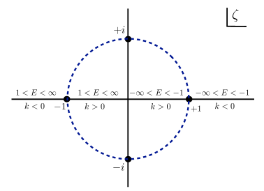
Figure 1: The spectral $\zeta$ plane, indicating the regions of positive and negative energy and momentum. We have set the mass scale $m=1$. Note that for $\zeta$ outside the unit circle the boost has a positive velocity, negative inside the unit circle. Bound states, having $|E|<1$, correspond to a $\zeta$ of magnitude 1, lying on the unit circle.

The boost parameter $\eta$, rapidity $\xi$ and velocity $v$ are related by:

$$\eta=e^{\xi}=\sqrt{\frac{1+v}{1-v}},\quad v=\frac{\eta^{2}-1}{\eta^{2}+1}$$ (13)

Under a Lorentz boost, the light-cone variables transform as:

$$z\to\eta z,\quad\bar{z}\to\eta^{-1}z,\quad\zeta\to\eta\zeta$$ (14)

and the Lorentz scalar argument of a plane wave is written as:

$$k_{\mu}x^{\mu}=-\frac{1}{2}\left(\zeta\bar{z}-\frac{z}{\zeta}\right)$$ (15)

In terms of these variables, and in terms of the complex condensate (5), the Dirac equation for the two-component spinor ($\psi_{1}=\psi_{L},\psi_{2}=\psi_{R}$) reads:

$$2i\bar{\partial}\psi_{2}=\Delta\psi_{1}\quad,\quad 2i\partial\psi_{1}=-\Delta^{*}\psi_{2}$$ (16)

II General TDHF solution

II.1 Transparent potential

In a recent paper, a large class of transparent, time-dependent, scalar-pseudoscalar Dirac potentials has been constructed Dunne:2013tr . The method used was a generalization of the method invented by Kay and Moses for finding all static, transparent Schrödinger potentials kaymoses . We collect the main results, referring to Ref. Dunne:2013tr for proofs and more details. We make the following ansatz for the continuum spinor

$$\psi_{\zeta}=\frac{1}{\sqrt{1+\zeta^{2}}}\left(\begin{array}[]{c}\zeta\chi_{1}\\ -\chi_{2}\end{array}\right)e^{i(\zeta\bar{z}-z/\zeta)/2},$$ (17)

where $\chi_{1}$ and $\chi_{2}$ approach some constant for $x\to\infty$. In that case, the continuum spinor behaves like a plane wave travelling to the right for $x\to-\infty$, as well as for $x\to\infty$ (for $k>0$); hence it is manifestly reflectionless.

The basic ingredients in the construction of $\Delta$ and $\psi_{\zeta}$ are $N$ “plane wave” factors $e_{n},f_{n}$, with complex spectral parameters $\zeta_{n}$,

$$e_{n}=e^{i(\zeta_{n}^{*}\bar{z}-z/\zeta_{n}^{*})/2},\quad f_{n}=\frac{e_{n}}{\zeta_{n}^{*}},\quad n=1,...,N$$ (18)

$N$ is the number of bound states. The reduced spinor components $\chi_{1,2}$ in (17) are written as finite sums with $N$ poles:

$$\chi_{1} = 1+i\sum_{n=1}^{N}\frac{1}{\zeta-\zeta_{n}}e_{n}^{*}\phi_{1,n},$$

$$\chi_{2} = 1-i\sum_{n=1}^{N}\frac{\zeta}{\zeta-\zeta_{n}}e_{n}^{*}\phi_{2,n},$$ (19)

Here $\phi_{1,n}$ and $\phi_{2,n}$ are 2$N$ functions defined as the solutions of the following systems of linear, algebraic equations,

$$\sum_{m=1}^{N}\left(\omega+B\right)_{nm}\phi_{1,m} = e_{n},$$

$$\sum_{m=1}^{N}\left(\omega+B\right)_{nm}\phi_{2,m} = -f_{n}.$$ (20)

Here, $\omega$ is a constant, hermitean but otherwise arbitrary $N\times N$ matrix, and $B$ is an $N\times N$ matrix constructed from the basis functions, $e_{n}(z,\bar{z})$, and spectral parameters, $\zeta_{n}$, as follows:

$$B_{nm}=i\frac{e_{n}e_{m}^{*}}{\zeta_{m}-\zeta_{n}^{*}}.$$ (21)

The $\zeta_{n}$ can be identified with the positions of the bound state poles of $\psi_{\zeta}$ in the complex $\zeta$-plane, see Eq. (19). To simplify the notation, we denote by $e,f,\phi_{1},\phi_{2}$ the $N$-dimensional vectors with components $e_{n},f_{n},\phi_{1,n},\phi_{2,n}$, respectively, whereas $\omega$ and $B$ denote $N\times N$ matrices. Eq. (20) becomes

$$(\omega+B)\phi_{1} = e,$$

$$(\omega+B)\phi_{2} = -f.$$ (22)

As shown in Ref. Dunne:2013tr , the $\phi_{n}$ are $N$ bound state spinors and $\psi_{\zeta}$ is the continuum spinor belonging to the transparent Dirac potential

$$\Delta=1-ie^{\dagger}\phi_{2}=1+i\phi_{1}^{\dagger}f=1+ie^{\dagger}\frac{1}{\omega+B}f.$$ (23)

The three different expressions for $\Delta$ given here are equivalent owing to Eq. (22). Let us introduce a 3rd vector $g$ in addition to $e,f$ defined in Eq. (18), with components

$$g_{n}=\frac{e_{n}}{\zeta-\zeta_{n}^{*}}.$$ (24)

This yields more compact expressions for $\chi_{1},\chi_{2}$ as well,

$$\chi_{1} = 1+ig^{\dagger}\phi_{1},$$

$$\chi_{2} = 1-i\zeta g^{\dagger}\phi_{2}.$$ (25)

Furthermore, simple expressions in terms of determinants have been presented in Dunne:2013xta ; Dunne:2013tr for the condensate $\Delta$ and the spinor components $\chi_{1,2}$.

The bound state spinors $\phi_{n}$ are in general neither orthogonal nor normalized. A set of properly orthonormalized spinors can be constructed via

$$\hat{\phi}_{n}=\sum_{m=1}^{N}C_{nm}\phi_{m},\quad\int_{-\infty}^{\infty}dx\hat{\phi}_{n}^{\dagger}\hat{\phi}_{m}=\delta_{n,m}.$$ (26)

As shown in Dunne:2013tr , the matrix $C$ then satisfies the condition,

$$2C\omega^{-1}C^{\dagger}=1.$$ (27)

This was derived under the assumption that ${\rm Im}\,k_{n}>0$, where

$$k_{n}=\frac{1}{2}\left(\zeta_{n}-\frac{1}{\zeta_{n}}\right)$$ (28)

is the complex momentum belonging to the $n$-th bound state. The following asymptotic behavior of the potential was found in Dunne:2013tr ,

$$\lim_{x\to-\infty}\Delta=1,\quad\lim_{x\to\infty}\Delta=\prod_{n=1}^{N}\frac{\zeta_{n}}{\zeta_{n}^{*}}=e^{i\Theta}.$$ (29)

This shows that $\Delta$ has a chiral twist $e^{i\Theta}$ where the chiral twist angle $\Theta$ can be computed by simply adding up the phases of all bound state pole parameters $\zeta_{n}$,

$$\Theta=2\sum_{n=1}^{N}\theta_{n},\qquad\zeta_{n}=|\zeta_{n}|e^{i\theta_{n}}.$$ (30)

The spinor components have the asymptotic behavior

$$\lim_{x\to-\infty}\chi_{1} = 1,\quad\lim_{x\to\infty}\chi_{1}=\prod_{n=1}^{N}\frac{\zeta-\zeta_{n}^{*}}{\zeta-\zeta_{n}},$$ (31)

$$\lim_{x\to-\infty}\chi_{2} = 1,\quad\lim_{x\to\infty}\chi_{2}=\prod_{n=1}^{N}\frac{\zeta_{n}}{\zeta_{n}^{*}}\frac{\zeta-\zeta_{n}^{*}}{\zeta-\zeta_{n}}.$$ (32)

From Eq. (31) we can read off the fully factorized, unitary transmission amplitude $T(\zeta)$ with the expected pole structure,

$$T(\zeta)=\prod_{n=1}^{N}\frac{\zeta-\zeta_{n}^{*}}{\zeta-\zeta_{n}},\qquad|T(\zeta)|=1.$$ (33)

The extra factors in the product in (32) are due to the chiral twist of the potential $\Delta$ which also affects the spinors.

II.2 Self-consistency

We now show that this solution also gives a self-consistent solution to the fully quantized TDHF problem (4), provided certain filling-fraction conditions are satisfied by the combined soliton-fermion system, generalizing the conditions already found by DHN and Shei Dashen:1974ci ; Shei:1976mn . The TDHF potential $\Delta$ receives contributions from the Dirac sea and the valence bound states,

$$\Delta=-2Ng^{2}\left(\langle\psi_{1}^{*}\psi_{2}\rangle_{\rm sea}+\langle\psi_{1}^{*}\psi_{2}\rangle_{\rm b}\right),$$ (34)

with

$$\langle\psi_{1}^{*}\psi_{2}\rangle_{\rm sea} = -\frac{1}{2}\int_{1/\Lambda}^{\Lambda}\frac{d\zeta}{2\pi}\frac{1}{\zeta}\chi_{1}^{*}\chi_{2},$$ (35)

$$\langle\psi_{1}^{*}\psi_{2}\rangle_{\rm b} = \sum_{n}\nu_{n}\hat{\phi}_{1,n}^{*}\hat{\phi}_{2,n}.$$ (36)

The integration limits in (35) correspond to a symmetric momentum cutoff $\pm\Lambda/2$ in ordinary coordinates. We insert the expressions for $\chi_{1},\chi_{2}$ from (25) and isolate the $\zeta$-dependence of the integrand in the continuum part (35). The integrand contains only simple poles in the complex $\zeta$-plane, so that the integration over $d\zeta$ with a cutoff can easily be performed. The pole at $\zeta=0$ yields the divergent contribution

$$\left.\langle\psi_{1}^{*}\psi_{2}\rangle_{\rm sea}\right|_{\rm div}=-\frac{\Delta}{2\pi}\ln\Lambda.$$ (37)

If one inserts this into (34) and uses the vacuum gap equation

$$\frac{Ng^{2}}{\pi}\ln\Lambda=1,$$ (38)

one finds that this part gives self-consistency by itself. Requiring that the convergent part of the sea contribution cancels the bound state contribution should give us the relationship between the bound state occupation fractions $\nu_{n}$ and the parameters of the solution, provided the solution is self-consistent. The computation of the convergent part of the sea contribution is straightforward. To present the result in a concise form, we introduce a diagonal matrix $M$,

$$M_{nm}=-i\delta_{nm}\ln(-\zeta_{n}^{*}).$$ (39)

(Logarithms of $\zeta_{n}$ appear if one integrates over $d\zeta$, as a result of the simple poles in the complex $\zeta$ plane.) The convergent part of (35) can then be simplified to

$$\left.\langle\psi_{1}^{*}\psi_{2}\rangle_{\rm sea}\right|_{\rm conv}=-\frac{1}{4\pi}\phi_{1}^{\dagger}\left(\omega M^{\dagger}+M\omega\right)\phi_{2}$$ (40)

The bound state contribution (36) is evaluated with the help of Eq. (27). After introducing another diagonal matrix $N$,

$$N_{nm}=4\pi\delta_{nm}\nu_{n},$$ (41)

it can be written as

$$\langle\psi_{1}^{*}\psi_{2}\rangle_{\rm b}=\frac{1}{4\pi}\phi_{1}^{\dagger}\left(C^{\dagger}NC\right)\phi_{2}.$$ (42)

Expressions (40) and (42) cancel if we require that

$$\omega M^{\dagger}+M\omega=C^{\dagger}NC.$$ (43)

This is the self-consistency relation determining the bound state occupation fractions. It can be cast into a more convenient form by combining Eqs. (27) and (43) as follows. From our experience with concrete applications of this formalism, it appears that $\omega$ should be chosen as a positive definite matrix to avoid singularities in $\Delta$ as a function of $(x,t)$. Assuming that $\omega$ is positive definite, it has the unique Cholesky decomposition

$$\omega=LL^{\dagger}$$ (44)

where $L$ is a lower triangular matrix. From (27) we conclude that the matrix

$$V=\sqrt{2}C\frac{1}{L^{\dagger}}$$ (45)

is unitary. The self-consistency condition (43) can then be transformed into the final form

$$2\left(L^{\dagger}M^{\dagger}\frac{1}{L^{\dagger}}+\frac{1}{L}ML\right)=V^{\dagger}NV.$$ (46)

Thus, the eigenvalues of the matrix on the left hand side of (46) determine the diagonal entries of the matrix $N$, which yield the fermion filling fractions $\nu_{n}$ in (41). To test whether a given candidate solution is self-consistent, one has to confirm that all eigenvalues are between 0 and $4\pi$, thereby satisfying the self-consistency condition with physical occupation fractions $\nu_{n}\in[0,1]$. As an alternative to the Cholesky decomposition, Eq. (46) remains valid if one replaces $L$ by $\sqrt{\omega}$, which can be computed by diagonalizing $\omega$ first.

II.3 Vanishing fermion density

Due to strong constraints from chiral symmetry in 1+1 dimensions, the massless NJL₂ model does not allow any localized fermion density or current Karbstein:2007 . Similarly, there is no localized energy or momentum density Brendel:2010 . This follows from the conservation laws

$$\partial_{\mu}j_{V}^{\mu}=0,\qquad\partial_{\mu}j_{A}^{\mu}=0,\qquad\partial_{\mu}{\cal T}^{\mu\nu}=0$$ (47)

together with the fact that

$$j_{V}^{0} = j_{A}^{1}=\psi^{\dagger}\psi,\qquad j_{V}^{1}=j_{A}^{0}=\psi^{\dagger}\gamma_{5}\psi$$

$${\cal T}^{00} = {\cal T}^{11}={\cal H},\qquad{\cal T}^{01}={\cal T}^{10}={\cal P}$$ (48)

in the massless NJL₂ model. The conservation laws (47) remain valid in TDHF approximation. Since the bound states carry lumps of localized fermions, there must be an exact cancellation between continuum states and bound states for all of these densities. As a consistency test of the above TDHF solution, let us check this cancellation explicitly for the simplest case, the fermion density $\rho=j_{V}^{0}$. The induced fermion density in the Dirac sea is

$$\rho_{\rm ind}=\int_{0}^{\infty}\frac{d\zeta}{2\pi}\frac{\zeta^{2}+1}{2\zeta^{2}}\left(\psi_{\zeta}^{\dagger}\psi_{\zeta}-1\right)=\frac{1}{2}\int_{0}^{\infty}\frac{d\zeta}{2\pi}\left\{\left|\chi_{1}\right|^{2}-1+\frac{1}{\zeta^{2}}\left(\left|\chi_{2}\right|^{2}-1\right)\right\}.$$ (49)

If we replace $\chi_{1},\chi_{2}$ by the expressions given in (25), we can simplify the result after some straightforward computations to

$$\rho_{\rm ind}=\partial_{x}\int_{0}^{\infty}\frac{d\zeta}{2\pi}g^{\dagger}\frac{1}{\omega+B}g.$$ (50)

Inserting the $g$’s and performing the integration over $d\zeta$, the result can be written as

$$\rho_{\rm ind}=\frac{1}{2\pi}{\rm Tr}\left[\left(\omega M^{\dagger}+M\omega\right)\partial_{x}\frac{1}{\omega+B}\right].$$ (51)

The density from the bound states with occupation fractions $\nu_{n}$ yields Dunne:2013tr

$$\rho_{b}=\sum_{n}\nu_{n}\hat{\phi}_{n}^{\dagger}\hat{\phi}_{n}=-\frac{1}{2\pi}{\rm Tr}\left[\left(C^{\dagger}NC\right)\partial_{x}\frac{1}{\omega+B}\right]$$ (52)

If the self-consistency condition (43) is satisfied, the bound state density (52), and the induced fermion density in the sea (51) cancel exactly. The vanishing of the current density $j_{V}^{1}$ can be proven in a similar manner, the only difference being that $\partial_{x}$ gets replaced by $\partial_{t}$ everywhere.

II.4 Time delays and masses

In standard soliton theory, the outcome of a scattering process is expressed via the time delay experienced by the solitons during the collision. As already discussed in Fitzner:2012gg , the situation is more complicated if multi-soliton bound states are involved. In this case the shape of the bound state may be affected as well. In the present work, we face the additional complication that the phases entering the breather oscillation may be changed during the scattering process. The best way to define the outcome of such a scattering process of composite multi-soliton objects is to compare the potential $\Delta$ for a cluster of kinks moving with a common velocity $v_{0}$ before and after the collision. Inspection of a few cases with small number of kinks shows the following general pattern: The change in $\Delta$ for a cluster involving $K$ kinks consists of an overall twist factor $\tau$ and rescalings of all the elementary functions $e_{n}$ by complex numers $\lambda_{n}$,

$$\Delta_{\rm out}(e_{i_{1}},...,e_{i_{K}})=\tau\Delta_{\rm in}(\lambda_{i_{1}}e_{i_{1}},...,\lambda_{i_{K}}e_{i_{K}})$$ (53)

with

$$\tau = \prod_{n(v_{n}<v_{0})}\frac{\zeta_{n}}{\zeta_{n}^{*}}\prod_{m(v_{m}>v_{0})}\frac{\zeta_{m}^{*}}{\zeta_{m}},$$

$$\lambda_{n} = \prod_{m(v_{m}<v_{0})}\left(\frac{\zeta_{n}^{*}-\zeta_{m}^{*}}{\zeta_{n}^{*}-\zeta_{m}}\right)\prod_{k(v_{k}>v_{0})}\left(\frac{\zeta_{n}^{*}-\zeta_{k}}{\zeta_{n}^{*}-\zeta_{k}^{*}}\right)$$ (54)

Alternatively, one could interpret the rescalings of the $e_{n}$ as a modification of the matrix $\omega^{0}$ of the cluster (one block out of the full, block-diagonal matrix $\omega$),

$$\left.\omega_{nm}^{0}\right|_{\rm out}=\frac{\left.\omega_{nm}^{0}\right|_{\rm in}}{\lambda_{n}\lambda_{m}^{*}}.$$ (55)

The twist factor $\tau$ can readily be understood in terms of the chiral twists of the solitons involved in the scattering process. The elementary factors entering the expression for $\lambda_{n}$ also have a simple interpretation. The transmission amplitude of a fermion with spectral parameter $\zeta$ scattering off soliton $m$ is

$$T_{m}(\zeta)=\frac{\zeta-\zeta_{m}^{*}}{\zeta-\zeta_{m}}.$$ (56)

Hence the factor $\lambda_{n}$ in (54) can be expressed in terms of transmission amplitudes of a fermion on all solitons not belonging to the cluster, evaluated at the complex spectral parameter $\zeta_{n}^{*}$, the complex conjugate of the bound state pole position,

$$\lambda_{n}=\prod_{m(v_{m}<v_{0})}T_{m}(\zeta_{n}^{*})\prod_{k(v_{k}>v_{0})}\frac{1}{T_{k}(\zeta_{n}^{*})}.$$ (57)

Another question of interest concerns the masses of clusters of solitons. In Ref. Brendel:2010 , a formula for the mass of TDHF solutions of the NJL₂ model was derived. Starting from Eqs. (47, 48) for the energy momentum tensor, it was found that the mass can be expressed in terms of the asymptotic behavior of the fermion phase shift for $k\to\infty$,

$$M=\frac{N}{\pi}\lim_{k\to\infty}k\delta(k).$$ (58)

Here, $\delta(k)$ is the phase of the (unimodular) fermion transmission amplitude $T(k)$. For a single twisted kink, this reproduces the original result of Shei Shei:1976mn ,

$$M_{1}=\frac{N}{\pi}\sin\varphi_{1},\qquad\zeta_{1}=-e^{-i\varphi_{1}}.$$ (59)

According to (33), the full transmission amplitude factorizes into fermion-kink transition amplitudes, hence the phase shifts are additive, as expected for integrable systems. This holds independently of whether the solitons form static bound states or breathers. Consequently, the mass of any compound of $n$ solitons is just the sum of the masses of the constituents — the binding energy vanishes. This is consistent with what has already been known for static bound states since Ref. Shei:1976mn , but generalizes to the breather case as well.

An interesting spinoff results if we apply these insights to real $\Delta$, i.e., TDHF solutions of the GN model. A two-kink bound state has the mass

$$M_{\rm kink}(\varphi_{1})+M_{\rm kink}(\pi-\varphi_{1})=\frac{2N}{\pi}\sin\varphi_{1}.$$ (60)

This relates the mass of the DHN baryon (or breather, for that matter) to the mass of the Shei kink ($\sin\varphi_{1}$ is the parameter $y$ in DHN). This is perhaps the most conspicuous manifestation of the long overlooked fact that twisted kinks are the (hidden) constituents of the DHN baryon.

III Explicit Examples

In this Section we illustrate the general solution to the TDHF problem (23, 25, 46) with several examples. We classify the applications according to the number of bound states or, equivalently, the number of poles of the continuum spinors in the complex $\zeta$-plane.

III.1 General solution with one pole: twisted kink

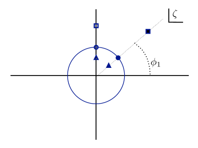
Figure 2: A spectral $\zeta$ plane representation of single kinks. Each of the open square, circle and triangle on the positive imaginary axis represents a real GN₂ kink, with positive, zero or negative boost, with respect to the rest frame. Each of the full square, circle and triangle on the ray at angle $\phi_{1}$ represents a complex twisted NJL₂ kink with phase parameter $\phi_{1}$. Taken together, all these six points represent the scattering of six kinks, 3 of them real and 3 with (equal) twist parameter $\phi_{1}$.

With one pole, the matrix $\omega$ is just a real number and the matrix $B$ reduces to a single function of $z,\bar{z}$. We parameterize the position $\zeta_{1}$ of the pole as

$$\zeta_{1}=-\frac{e^{-i\varphi_{1}}}{\eta_{1}},\quad\eta_{1}=\sqrt{\frac{1+v_{1}}{1-v_{1}}}.$$ (61)

The complex potential $\Delta$ can then be written as

$$\Delta=\frac{1+e^{-2i\varphi_{1}}U_{1}}{1+U_{1}}$$ (62)

with the real function

$$U_{1}=\frac{B_{11}}{\omega_{11}}=\frac{\eta_{1}}{2\omega_{11}\sin\varphi_{1}}\exp\left\{\frac{\sin\varphi_{1}}{\eta_{1}}(\bar{z}+\eta_{1}^{2}z)\right\}.$$ (63)

Expressed in ordinary coordinates, the argument of the exponential in $U_{1}$ reads

$$\frac{\sin\varphi_{1}}{\eta_{1}}(\bar{z}+\eta_{1}^{2}z)=2\sin\varphi_{1}\frac{x-v_{1}t}{\sqrt{1-v_{1}^{2}}}.$$ (64)

This is the boosted form of the Shei twisted kink (7) for the NJL₂ model. The role of the free parameter $\omega_{11}$ is to shift the position of the kink. The phase and modulus of $\zeta_{1}$ are related to the chiral twist and the velocity of the kink, respectively, as illustrated in Fig. 2. To cover the full range of chiral twists it is sufficient to restrict $\varphi_{1}$ to the interval $[0,\pi]$. In this case, $\sin\varphi_{1}>0$ and we have to choose $\omega_{11}>0$ in order to get a nonsingular $\Delta$. Notice that this definition of $\varphi_{1}$ also implies ${\rm Im}\,k_{1}>0$, as assumed in Dunne:2013tr . Turning to the self-consistency issue, the matrix $M$ introduced in (39) has just one component: $M_{11}=-i\,\ln(-\zeta_{1}^{*})=\varphi_{1}+i\,\ln\eta_{1}$. Thus, the NJL₂ filling fraction condition (46) gives:

$$\nu_{1}=\frac{\varphi_{1}}{\pi}$$ (65)

This self-consistent TDHF kink binds a number $n_{v}$ of valence fermions, where in the large $N_{f}$ limit the filling fraction $\nu_{1}=n_{v}/N_{f}$ is equal to the twist angle $\varphi_{1}$ divided by $\pi$.

We obtain the real kink solution (6) of GN₂ by choosing $\varphi_{1}=\frac{\pi}{2}$ in (62, 63). For GN₂ there is no filling fraction condition, as we do not have to impose a self-consistency condition on the pseudo scalar condensate.

In an $(S,P)$-plot, the twisted kink traces out a segment of a straight line, joining two points on the chiral circle. In our case, the starting point ($x\to-\infty$) is always the point $(S=1,P=0)$, whereas the endpoint ($x\to\infty$) depends on the chiral twist. Most of the examples discussed below are based on constituent kinks with parameters $\varphi_{1}$ = 1.0, 0.8, 0.6, 0.4, shown in Fig. 3 and, in greater detail, in the ancillary files to this paper (see 3dplot$\_$constituent$\_$kinks).

Figure 3: ($S,P$)-plot, of the scalar ($S$) and pseudoscalar ($P$) components of the condensate $\Delta$, for the four basic twisted kinks used to build up most of the multi-kink configurations in this work, as explained in the text.

III.2 General solution with two poles: kinks, baryons and breathers

With two poles, the matrices entering the general solution (23, 25, 46) are $2\times 2$. This enables us to work out everything explicitly, including the self-consistency condition. The physics depends on the assumptions about the constant matrix $\omega$ and the pole positions $\zeta_{1,2}$.

III.2.1 Non-breather solutions

We find non-breather solutions by choosing a diagonal form of $\omega$ in (23). Introducing functions $U_{i}=B_{ii}/\omega_{ii}$ for $i=1,2$ in analogy to (63) and generalizing the parameterization (61) to $\zeta_{1,2}$, we find the potential

$$\Delta=\frac{1+e^{-2i\varphi_{1}}U_{1}+e^{-2i\varphi_{2}}U_{2}+b_{12}e^{-2i(\varphi_{1}+\varphi_{2})}U_{1}U_{2}}{1+U_{1}+U_{2}+b_{12}U_{1}U_{2}}.$$ (66)

The interaction effects between the two twisted kinks are described by the real parameter $b_{12}$ given by

$$b_{12}=\left|\frac{\zeta_{1}-\zeta_{2}}{\zeta_{1}-\zeta_{2}^{*}}\right|^{2}=\frac{\eta_{1}^{2}+\eta_{2}^{2}-2\eta_{1}\eta_{2}\cos(\varphi_{1}-\varphi_{2})}{\eta_{1}^{2}+\eta_{2}^{2}-2\eta_{1}\eta_{2}\cos(\varphi_{1}+\varphi_{2})}.$$ (67)

This is the $N=2$ case of a general formula valid for diagonal $\omega$, presented in Sect. IIIB of Dunne:2013tr . Eq. (66) gives the self-consistent potential for the scattering of two twisted kinks, with twist angles $\varphi_{1}$ and $\varphi_{2}$, and boost parameters $\eta_{1}$ and $\eta_{2}$, or for a bound state if one chooses $\eta_{1}=\eta_{2}$. The filling-fraction consistency condition is simple when $\omega$ is diagonal. The $M$ matrix is $M={\rm diag}(\varphi_{1}+i\,\ln\eta_{1},\varphi_{2}+i\,\ln\eta_{2})$. Thus, we find filling fractions

$$\nu_{1}=\frac{\varphi_{1}}{\pi}\quad,\quad\nu_{2}=\frac{\varphi_{2}}{\pi},$$ (68)

as expected from the asymptotics of the scattering problem. If we are interested in solutions of the NJL₂ model with real $\Delta$, we are restricted to fermion number 0. In that case the self-consistency condition yields

$$\nu_{1}=\frac{\varphi_{1}}{\pi},\quad\nu_{2}=\frac{\varphi_{2}}{\pi}=\frac{\pi-\varphi_{1}}{\pi}=1-\nu_{1}$$ (69)

This corresponds to an “exciton” in condensed matter language. In the GN case, we cannot take over the derivation of the self-consistency condition which was only valid for generic parameters. Now, the contributions of the 2 bound states give equal and opposite contributions to the condensate $\bar{\psi}{\psi}$, so that only the difference of the corresponding two equations of the NJL₂ model survives,

$$\nu_{1}-\nu_{2}=\frac{\varphi_{1}-\varphi_{2}}{\pi}=\frac{2\varphi_{1}}{\pi}-1$$ (70)

The baryon state of lowest energy for given baryon number has fully occupied negative energy bound state, corresponding to $\nu_{2}=1,\nu_{1}=2\varphi_{1}/\pi$. This is the relation familiar from DHN.

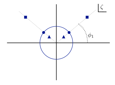
Figure 4: A spectral $\zeta$ plane representation of a real GN₂ baryon. The baryon is composed of two twisted kinks, one with chiral angle $\phi_{1}$, and the other with $\pi-\phi_{1}$. The triangles (squares) have $\zeta_{1}<1$ ($\zeta_{1}>1$), corresponding to negative (positive) boost parameter, while the circles correspond to a baryon at rest.

We can consider various special cases:

1. Scattering of two GN₂ kinks. We obtain real kink solutions by setting $\varphi_{1}=\varphi_{2}=\frac{\pi}{2}$. Then

   $$S=\frac{1-U_{1}-U_{2}+b_{12}U_{1}U_{2}}{1+U_{1}+U_{2}+b_{12}U_{1}U_{2}},\quad b_{12}=\left(\frac{\eta_{1}-\eta_{2}}{\eta_{1}+\eta_{2}}\right)^{2},$$ (71)

   and $\sin\varphi_{1,2}=1$ in the definition of $U_{1,2}$. This agrees with the $n=2$ case of the general formula in Fitzner:2010nv . There is no filling-fraction consistency condition.

2. GN₂ baryon. We can also obtain a real solution by choosing $\varphi_{2}=\pi-\varphi_{1}$, together with $\omega_{11}=\omega_{22}$. To obtain a baryon we also choose $\eta_{1}=\eta_{2}$. Then $U_{1}=U_{2}$ and we find

   $$S=\frac{1+2\cos(2\varphi_{1})U_{1}+\cos^{2}\varphi_{1}U_{1}^{2}}{1+2U_{1}+\cos^{2}\varphi_{1}U_{1}^{2}}$$ (72)

   which agrees with the GN₂ baryon in (8). Thus, we see that the DHN GN₂ baryon is in fact a bound pair of two twisted kinks, as depicted in Fig 4. The fermion filling-fractions are $\nu_{2}=1,\nu_{1}=2\varphi_{1}/\pi$, as in DHN. Note that DHN have written the parameter $y$ which defines the size of the baryon in the form $y=\sin\theta$, without geometrical interpretation of the angle $\theta$. Now we see that $\theta$ is nothing but the angle $\varphi_{1}$ related to the twist of the constituent kinks. These constituents are well hidden inside the baryon, since the individual twisted kinks are not solutions of the GN model. The only observable which hints at this compositeness is the factorized fermion transmission amplitude.

Figure 5: ($S,P$)-plot of a 2-kink, a bound state of two twisted kinks.

Figure 6: ($S,P$)-plot of a 2-breather made out of two kinks with the same parameters as the bound state in Fig. 5. The different curves illustrate the time dependence of the twisted breather, in equal time steps.

Figure 7: ($S,P$)-plot of the scattering process of two twisted kinks. The curves show the time dependence, in equal time steps. The initial and final states are open polygons with 2 segments, ending on the chiral circle.

III.2.2 Breather Solutions

Breather solutions in the rest frame are obtained by choosing $\eta_{1}=\eta_{2}=1$ and a non-diagonal $2\times 2$ matrix $\omega$ in (30, 46). Using the freedom of making translations in $x$ and $t$, we choose the following positive definite hermitean matrix:

$$\omega=\pmatrix{\sec\chi&\tan\chi\cr\tan\chi&\sec\chi}$$ (73)

Then we find for the GN₂ system where $\varphi_{2}=\pi-\varphi_{1}$:

$$S = \frac{\cal N}{\cal D}$$

$${\cal N} = 1+\frac{\cos(2\varphi_{1})}{\sin\varphi_{1}\cos\chi}e^{2x\sin\varphi_{1}}+\tan\chi e^{2x\sin\varphi_{1}}\sin(2t\cos\varphi_{1}+\varphi_{1})+\frac{1}{4}\cot^{2}\varphi_{1}e^{4x\sin\varphi_{1}}$$

$${\cal D} = 1+\frac{1}{\sin\varphi_{1}\cos\chi}e^{2x\sin\varphi_{1}}-\tan\chi e^{2x\sin\varphi_{1}}\sin(2t\cos\varphi_{1}+\varphi_{1})+\frac{1}{4}\cot^{2}\varphi_{1}e^{4x\sin\varphi_{1}}$$ (74)

This agrees (modulo translations in $x$ and $t$) with the DHN GN₂ breather (9) if we use the following identifications,

$$\epsilon=\tan\varphi_{1},\qquad b=\frac{1}{\cos\varphi_{1}\cos\chi},\qquad a=\tan\varphi_{1}\tan\chi.$$ (75)

The limit $\chi\to 0$ of (74) yields back the static DHN baryon (72) up to a shift in $x$, as can be seen by setting

$$U_{1}=\frac{e^{2x\sin\varphi_{1}}}{2\sin\varphi_{1}}.$$ (76)

A new twisted breather for the NJL₂ model is obtained by choosing the off-diagonal mixing matrix (73), and relaxing the reality condition (so that $\varphi_{2}\neq\pi-\varphi_{1}$) on the twist angles. This is the most complicated TDHF solution with two poles. In order to exhibit its structure, we first write down the potential $\Delta$ in the form

$$\Delta = \frac{\cal N}{\cal D}$$

$${\cal N} = 1+\frac{1}{\cos\chi}\left(\frac{\zeta_{1}}{\zeta_{1}^{*}}U_{1}+\frac{\zeta_{2}}{\zeta_{2}^{*}}U_{2}\right)+b_{12}\frac{\zeta_{1}\zeta_{2}}{\zeta_{1}^{*}\zeta_{2}^{*}}U_{1}U_{2}-\tan\chi\left(\frac{\zeta_{2}}{\zeta_{1}^{*}}B_{12}+\frac{\zeta_{1}}{\zeta_{2}^{*}}B_{21}\right)$$

$${\cal D} = 1+\frac{1}{\cos\chi}\left(U_{1}+U_{2}\right)+b_{12}U_{1}U_{2}-\tan\chi\left(B_{12}+B_{21}\right)$$ (77)

with $U_{1}=B_{11},U_{2}=B_{22}$, $B_{nm}$ from (21) and $b_{12}$ from (67). In the limit $\chi\to 0$, we recover the bound state of twisted kinks, see (66). The chiral twist of the solution is time independent and can be inferred from the prefactors of the $U_{1}U_{2}$ terms. It does not depend on $\chi$ and therefore coincides with the sum of the individual twists, like for the bound state. Consider the oscillating terms in ${\cal N}$ and ${\cal D}$ first, i.e., those multiplied by $\tan\chi$. Using ordinary coordinates to exhibit their space and time dependence, the factors multiplying $\tan\chi$ can be cast into the form

$$\left(\frac{\zeta_{2}}{\zeta_{1}^{*}}B_{12}+\frac{\zeta_{1}}{\zeta_{2}^{*}}B_{21}\right) = e^{-i(\varphi_{1}+\varphi_{2})}(B_{12}+B_{21}),$$

$$(B_{12}+B_{21}) = -\frac{2e^{Kx}}{\sqrt{K^{2}+\Omega^{2}}}\sin\left(\Omega t+\arctan\frac{K}{\Omega}\right),$$ (78)

where we have introduced a wave number $K$ and frequency $\Omega$ generalizing the corresponding quantities from the (real) DHN breather,

$$K=\sin\varphi_{1}+\sin\varphi_{2},\qquad\Omega=\cos\varphi_{1}-\cos\varphi_{2}.$$ (79)

The period of the twisted breather is $T=2\pi/\Omega$. The time independent parts of ${\cal N}$ and ${\cal D}$ can be evaluated with the help of

$$U_{1}=\frac{e^{2x\sin\varphi_{1}}}{2\sin\varphi_{1}},\qquad U_{2}=\frac{e^{2x\sin\varphi_{2}}}{2\sin\varphi_{2}},\qquad b_{12}=\frac{1-\cos(\varphi_{1}-\varphi_{2})}{1-\cos(\varphi_{1}+\varphi_{2})}.$$ (80)

Let us now turn to the issue of self-consistency. Following the steps leading to (46), we write $\omega$ in its Cholesky factorized form

$$\omega=\pmatrix{\sec\chi&\tan\chi\cr\tan\chi&\sec\chi}=LL^{\dagger}\quad,\quad L=\pmatrix{\sqrt{\sec\chi}&0\cr\sqrt{\cos\chi}\tan\chi&\sqrt{\cos\chi}}$$ (81)

Then

$$2\left(L^{\dagger}M^{\dagger}\frac{1}{L^{\dagger}}+\frac{1}{L}ML\right)=2\pmatrix{2\varphi_{1}&-(\varphi_{1}-\varphi_{2})\tan\chi\cr-(\varphi_{1}-\varphi_{2})\tan\chi&2\varphi_{2}}$$ (82)

Using (46), the eigenvalues of this matrix give the two filling fractions as:

$$\nu_{\pm}=\frac{\varphi_{1}+\varphi_{2}}{2\pi}\pm\frac{\varphi_{1}-\varphi_{2}}{2\pi}\sec\chi.$$ (83)

The condition that $\nu_{\pm}\in[0,1]$ restricts the allowed range of $\chi$ for given twist angles $\varphi_{1},\varphi_{2}$.

We illustrate these various examples in a few cases, using $(S,P)$ plots. In Fig. 5, a 2-kink bound state at rest (parameters: $\varphi_{1}=1.0,\,\varphi_{2}=0.8,\,\omega_{11}=3,\,\omega_{22}=1/\omega_{11}$) is shown. If one increases the distance between the kinks by increasing $\omega_{11}$, one reaches eventually two static, non-interacting kinks which would show up as an open polygon made out of two of the straight line segments shown in Fig. 3. The breather with the same parameters as the 2-kink and $\chi=1.1$ is illustrated in Fig. 6, where the different curves correspond to equidistant time steps. Fig. 7 shows the scattering of two twisted kinks with $\varphi_{1}=1.0,\varphi_{2}=0.8$. The initial and final states consist of two straight line segments ending on the chiral circle. During the collision process (illustrated again by a sequence of equidistant time steps), the kinks interchange their order. Clearly, these static pictures can give only an incomplete view of the time dependent examples. A complete graphical representation requires animated plots, as provided in the ancillary files to this paper for the same parameters, see the Appendix and the files animation$\_$kink$\_$plus$\_$kink and animation$\_$2-breather.

III.3 Three pole solutions

In the preceding section we have discussed the TDHF solutions built out of two kinks in great detail. With increasing number of kinks (or poles in the complex $\zeta$-plane), both the number of different physical configurations and the complexity of these solutions increase rapidly. It is straightforward to generate these solutions with Computer Algebra (CA) using the general formalism and to check the self-consistency by a numerical diagonalization of a finite matrix. We will show examples of such calculations at the end of this and the following sections. We start with a survey of the different cases with 3 poles.

Figure 8: ($S,P$)-plot of a 3-kink, a bound state of 3 twisted kinks.

Figure 9: ($S,P$)-plot of the scattering of a 2-kink and a kink. The curves illustrate the time dependence, in equal time steps. Initial and final states can be identified by the fact that one inner point on a curve touches the chiral circle.

Figure 10: $(S,P$)-plot of the scattering process of 3 single, twisted kinks. The curves show the time dependence, in equal time steps. Initial and final states correspond to 3-sided open polygons, all corners and endpoints lying on the chiral circle.

The input to any TDHF calculation of the NJL₂ or GN models are a set of boost parameters $\eta_{n}$ and chiral twist angles $\varphi_{n}$ for the constituent kinks, together with the bound state mixing matrix $\omega$. These parameters are not entirely independent though. A non-vanishing off diagonal matrix element $\omega_{nm}$ implies that the physical bound states of kinks $n$ and $m$ get mixed. This is only physically meaningful if these two kinks have the same boost parameter $\eta_{n}=\eta_{m}$, since otherwise the two kinks would be arbitrarily far apart at asymptotic times and the mixing would violate cluster separability. The other restriction is that two kinks (not involved in breathers) with the same $\eta_{n}$ parameter must have different $\varphi_{n}$’s, otherwise the number of kinks is reduced by 1.

With this in mind, the possibilities with 3 kinks are as follows. If $\eta_{1},\eta_{2},\eta_{3}$ are all different, we are dealing with the scattering of 3 individual kinks. If one chooses in particular $\varphi_{n}=\pi/2$ for all 3 kinks, this reproduces known results for 3 CCGZ kinks of the GN model derived from the Sinh-Gordon solitons in Fitzner:2010nv . If two of the kinks have the same velocity (say $\eta_{1}=\eta_{2}\neq\eta_{3}$), we are dealing with the scattering of a two-kink compound and a single kink and we must choose $\omega_{13}=\omega_{23}=0$. The compound system can either be a bound state ($\omega_{12}=0$) or a breather ($\omega_{12}\neq 0$), as discussed in section III.2. In the case of real potentials, this includes scattering and bound states of a DHN breather or baryon ($\varphi_{2}=\pi-\varphi_{1}$) and a CCGZ kink ($\varphi_{3}=\pi/2$). The bound state case has been discussed independently in the condensed matter Okuno:1983 and particle physics Feinberg:2003 literature. Finally, if all 3 kinks have the same velocity, there are 3 possibilities for $\omega$: If $\omega$ is diagonal, we describe the 3-kink bound state which fits into the framework of Takahashi:2012pk . If only one off-diagonal element $\omega_{nm}$ is different from zero, this describes a bound state of a 2-kink breather (kinks $n,m$) and a single kink. If more than one off-diagonal elements $\omega_{nm}$ are different from zero, this three kink compound state cannot be resolved into a 2-kink breather and a kink, but represents a more complicated oscillation mode where all 3 kinks are involved in a non-trivial way. Of course, in all of these cases one has to check that the self-consistency condition can be fulfilled with physical occupation fractions $\nu_{n}\in[0,1]$. Since this involves diagonalization of a 3$\times$3 matrix, this has to be checked on a case-by-case basis.

In order to simplify the discussion in the next section, we introduce the following language: A bound state of $n$ twisted kinks will be referred to as “$n$-kink” (a “1-kink” being simply a kink). An irreducible breather made out of $n$ kinks will be called “$n$-breather”. If several clusters are scattering, this will be indicated by a + sign, e.g., kink + kink for the scattering of 2 kinks. Then the one pole solution deals with the kink, the two pole solution with kink + kink, 2-kink, 2-breather, and the three pole solution with kink + kink + kink, kink + 2-kink, kink + 2-breather, 3-kink, 3-breather.

Let us illustrate once again a few cases, using $(S,P)$ plots. In Fig. 8, a 3-kink bound state at rest (parameters: $\varphi_{1}=1.0,\,\varphi_{2}=0.8,\,\varphi_{3}=0.6,\,\omega_{11}=9,\,\omega_{22}=1,\,\omega_{33}=1/9$) is shown. Fig. 9 represents the scattering of a 2-kink bound state and a single kink ($\eta_{1}=\eta_{2}=2,\eta_{3}=1/2$), and Fig. 10 the scattering of three twisted kinks ($\eta_{1}=2,\,\eta_{2}=1,\,\eta_{3}=1/2$). Similar plots involving 2-breathers or 3-breathers are not really able to convey a picture of the complicated time dependence. We refer the reader to the Appendix and the ancillary files, where full animations of all of these cases can be found (animation$\_$kink$\_$plus$\_$kink$\_$plus$\_$kink, animation$\_$2-breather$\_$kink$\_$boundstate, animation$\_$2-breather$\_$plus$\_$kink, animation$\_$3-breather).

III.4 Four pole solutions

TDHF solutions based on four kinks are of particular interest, since we reach the level of complexity needed to describe baryon-baryon and breather-breather scattering in the GN model. These problems have already been solved recently by a different method based on an ansatz for the TDHF potential Dunne:2011wu ; Fitzner:2012kb , at the expense of a substantial technical effort. It is an important cross-check of the present simpler approach to reproduce these complicated results.

From the preceding discussion, it is clear that the various four kink processes can be classified as follows: kink + kink + kink + kink, kink + kink + 2-kink, kink + kink + 2-breather, 2-kink + 2-kink, 2-kink + 2-breather, 2-breather + 2-breather, kink + 3-kink, kink + 3-breather, 4-kink, 4-breather. Out of these, we select the following processes which are of interest for the GN model:

1. 2-kink + 2-kink

   By pairing the twist angles ($\varphi_{1}+\varphi_{2}=\varphi_{3}+\varphi_{4}=\pi$) and using a diagonal matrix $\omega$, this particular process can be turned into scattering of two DHN baryons studied in Dunne:2011wu . We have checked with CA that the present closed expressions reproduce exactly the results of Ref. Dunne:2011wu , provided one chooses the origin of the $x$ and $t$ axes appropriately. This calculation can now be generalized to the scattering of two twisted 2-kinks in a straightforward manner.

   

   Figure 11: ($S,P$)-plot of a 4-kink, a bound state of four twisted kinks.

   

   Figure 12: ($S,P$)-plot of the scattering process of two 2-kinks. The curves show the time dependence, in equal time steps. The initial and final states are the curves touching the chiral circle with an inner point.

2. 2-breather + 2-breather

   In order to get a real TDHF potential for breather-breather scattering, one has to pair the twist angles as in the baryon-baryon case and choose $\omega$ in the block diagonal form

   $$\omega=\pmatrix{\omega_{11}&\omega_{12}&0&0\cr\omega_{12}^{*}&\omega_{11}&0&0\cr 0&0&\omega_{33}&\omega_{34}\cr 0&0&\omega_{34}^{*}&\omega_{33}}$$ (84)

   Once again, we have checked with CA that the result agrees with the solution of breather-breather scattering in the GN model from Fitzner:2012kb . A comparison between the complicated formulas given in Fitzner:2012kb and the present work shows how efficient it is to take the detour via the NJL₂ model, where one can take full advantage of factorization and integrability properties of the model. Once again, the present approach allows us to repeat the calculation with twisted breathers in the NJL₂ model with modest effort, solving an even more complicated problem analytically.

3. 4-breather

   An irreducible four-kink breather of the NJL₂ model has many free parameters due to the appearance of a general, hermitean 4$\times$4 matrix $\omega$. We do not study all of these complex oscillation modes here, but ask the question: How many parameters survive if we specialize the 4-breather to real $\Delta$, i.e., a solution of the GN model? This is of some interest, since the 4-breather is the simplest TDHF solution of the GN model which cannot be reduced to the known basic building blocks of kink, baryon and 2-breather. (There is no real 3-breather, since the chiral twists have to be paired). We have computed the TDHF potential $\Delta$ for the 4-breather at rest with CA, using $\varphi_{1}+\varphi_{2}=\varphi_{3}+\varphi_{4}=\pi$ and keeping $\omega$ general at first. We then demand that $\Delta$ is real. This puts a number of constraints on the matrix elements $\omega_{nm}$. The most general solution can be parameterized as follows ($a$ and $e$ are real),

   $$\omega=\pmatrix{a&b&c&d\cr b^{*}&a&d^{*}&c^{*}\cr c^{*}&d&e&f\cr d^{*}&c&f^{*}&e}$$ (85)

   This leaves a lot of room for new kinds of solutions of the GN model, parameterized by the 2 complex parameters $c,d$ characteristic for an irreducible 4-breather.

In Fig. 11, a 4-kink bound state at rest (parameters: $\varphi_{1}=1.0,\,\varphi_{2}=0.8,\,\varphi_{3}=0.6,\,\varphi_{4}=0.4,\,\omega_{11}=81,\,\omega_{22}=9,\,\omega_{33}=1,\,\omega_{44}=1/9$) is illustrated. Fig. 12 shows the scattering of a 2-kink on a 2-kink. For animations of the complete time dependence and processes involving breathers, see the Appendix and the ancillary files (animation$\_$2-kink$\_$plus$\_$2-kink, animation$\_$2-breather$\_$plus$\_$2-breather, animation$\_$4-breather), where also an example of an irreducible 4-breather of the GN model with real $\Delta=S$ (animation$\_$real$\_$4-breather) can be found.

IV Summary and conclusions

Within one year after the inception of the GN₂ model, DHN found a time dependent multi-fermion solution, the breather Dashen:1974ci . They also realized that it is related to the kink-antikink scattering problem by analytic continuation. Somewhat surprisingly, no further progress was made on time-dependent solutions of either the GN₂ or the NJL₂ model between 1975 and 2010, to the best of our knowledge. In the present work and in Refs. Dunne:2013xta ; Dunne:2013tr , we have presented what we believe to be the full solution of the TDHF problem for both the GN₂ and NJL₂ models. Let us briefly summarize how this has been achieved.

In a first round of investigations starting in 2010, the interaction of a small number of scatterers was studied in great detail by means of an ansatz method. The scatterers involved were kinks Klotzek:2010gp , baryons Dunne:2011wu and breathers Fitzner:2012kb , all belonging to the GN₂ model. The ansatz consisted of multiplying the scalar potentials and spinors for the individual scatterers and then varying the coefficients of some ($x,t$)-dependent exponentials, until the Dirac equation was satisfied. This could be done at the expense of considerable use of computational algebra, and led to the exact solutions of the problems considered. In the course of these works, many simplifying features emerged which enabled the authors to extrapolate the results to more complicated scattering processes involving $N$ scatterers Fitzner:2012gg . Since a general proof was lacking, these results could only be checked analytically for few body problems, up to $N=6$. In the simplest special case, that of multi-kink scattering, the problem proved to be fully solvable for all $N$, by mapping it onto the known soliton solutions of the Sinh-Gordon equation Fitzner:2010nv .

Several developments have helped us to solve the problem in full generality in the meantime. Thus for instance, we realized that it is advantageous to solve the NJL₂ model first, and then get the GN₂ solutions in a second step by specializing to real TDHF potentials. This strategy had been overlooked for a long time, and is indeed unexpected: the NJL₂ model has a more complicated Lagrangian than the GN₂ model. Moreover, its continuous chiral symmetry forbids states with localized fermion density, whereas one is just interested in such “baryonic” states in the GN₂ model. The reason why the NJL₂ model is easier to solve lies in the fact that twisted kinks are the basic constituents of all TDHF solutions, and they appear in free form only in the NJL₂ model. Nevertheless, they are also hidden constituents of GN₂ baryons and breathers, as we have shown here. As for the question of fermion density, we have shown that the same construction of the TDHF potential can be used for both models, but the self-consistency condition is different, leading to different assignments of fermion number, but with the same condensate.

A two step procedure for solving the TDHF problem has proven most economic. In a first step, we have constructed a general family of transparent scalar-pseudoscalar Dirac potentials Dunne:2013tr , generalizing the method used for the stationary Schrödinger equation by Kay and Moses long ago kaymoses . This yields closed form expressions for processes involving $N$ twisted kinks. Depending on the parameters, they describe kinks, bound states, breathers and scattering processes among all of these entities. In a second step reported in the present paper, we employ these transparent potentials in a TDHF calculation and prove their self-consistency. While the method is completely general, it requires diagonalization of an $N\times N$ matrix. Thus, for more than $N=2$ it is difficult to write general analytic expressions, so the occupation fractions of the bound states are best determined numerically. We have presented examples with up to 4 kinks, displaying a rich spectrum of scenarios, in particular as far as breathers are concerned. If one specializes these examples to real potential, either by choosing the twist angle $\pi$ or by pairing two twisted kinks to total twist 0, one recovers all the preceding results from the GN₂ model. In contrast to the earlier works, we now have the general proof of the Dirac equation and self-consistency condition, as well as compact closed expressions in terms of determinants, valid for arbitrary numbers of constituent kinks. We have also learned that new kinds of breathers appear at each $N$, so that one cannot exhaust the dynamics of the GN₂ model via bound or scattering states of $N=2$ objects only. The basic constituent common to all solutions is the twisted kink, which does not exist as a free entity in the GN model — it is hidden.

Characteristic for integrable models is the fact that the transmission amplitude for a fermion on a compound object factorizes in the individual kink constituents. Nevertheless, there are nontrivial back-reaction effects which require fermion filling-fraction conditions for a self-consistent TDHF solution. We have shown that the factorized scattering translates into an additivity of the kink masses for all bound states and breathers. It is also the key for finding the asymptotic behavior of the solitons after the scattering has taken place. This includes in general a deformation of the soliton shape, a time delay and (for breathers) a change in the phases of the oscillations.

Is this the end of the story? Given the fact that all static HF solutions are known, the only loophole is for the breathers. We have not yet completely ruled out that the ansatz we have used for finding transparent Dirac potentials misses some exotic breathers with an even more complicated structure. However, in view of the simplicity of the underlying Lagrangians, this seems very unlikely.

V Appendix: Parameters used in the animations

Here we collect the parameters used in the animations contained in the Ancillary/Supplementary Material to the present paper, which can be found at the link on this paper’s arXiv page.

The fermion occupation fractions $\nu_{n}$ are not input, but the result of the self-consistency condition. For kinks, they can be computed as $\nu_{n}=\varphi_{n}/\pi$, therefore they are not given below. For solutions involving breathers, the fermion occupation numbers are derived from the eigenvalues in the consistency condition (46), as described at the end of section II.2.

• animation$\_$kink$\_$plus$\_$kink

  $$\eta_{1}=2,\quad\eta_{2}=1/2$$

  $$\varphi_{1}=1.0,\quad\varphi_{2}=0.8$$

  $$\omega_{11}=3,\quad\omega_{22}=1/3$$

• animation$\_$2-breather

  $$\eta_{1}=\eta_{2}=1$$

  $$\varphi_{1}=0.6,\quad\varphi_{2}=1.2$$

  $$\chi=1.1$$

  $$\nu_{1}=0.076,\quad\nu_{2}=0.497$$

• animation$\_$kink$\_$plus$\_$kink$\_$plus$\_$kink

  $$\eta_{1}=2,\quad\eta_{2}=1,\quad\eta_{3}=1/2$$

  $$\varphi_{1}=1.0,\quad\varphi_{2}=0.8,\quad\varphi_{3}=0.6$$

  $$\omega_{11}=9,\quad\omega_{22}=1,\quad\omega_{33}=1/9$$

• animation$\_$2-kink$\_$plus$\_$kink

  $$\eta_{1}=\eta_{2}=2,\quad\eta_{3}=1/2$$

  $$\varphi_{1}=1.0,\quad\varphi_{2}=0.8,\quad\varphi_{3}=0.6$$

  $$\omega_{11}=9,\quad\omega_{22}=1,\quad\omega_{33}=1/9$$

• animation$\_$2-breather$\_$kink$\_$boundstate

  $$\eta_{1}=\eta_{2}=\eta_{3}=1$$

  $$\varphi_{1}=1.0,\quad\varphi_{2}=0.8,\quad\varphi_{3}=0.6$$

  $$\chi=1.4,\quad\omega_{33}=1/81$$

  $$\nu_{1}=0.474,\quad\nu_{2}=0.099$$

• animation$\_$2-breather$\_$plus$\_$kink

  $$\eta_{1}=\eta_{2}=1.1,\quad\eta_{3}=1/\eta_{1}$$

  $$\varphi_{1}=1.0,\quad\varphi_{2}=0.8,\quad\varphi_{3}=0.6$$

  $$\chi=1.4,\quad\omega_{33}=1/81$$

  $$\nu_{1}=0.474,\quad\nu_{2}=0.099$$

• animation$\_$3-breather

  $$\eta_{1}=\eta_{2}=\eta_{3}=1$$

  $$\varphi_{1}=1.0,\quad\varphi_{2}=0.8,\quad\varphi_{3}=0.6$$

  $$L=\left(\begin{array}[]{rrr}2.5&0&0\\ 2.4&0.5&0\\ 1.65&-0.7&1.0\end{array}\right)$$ (89)

  $$\nu_{1}=0.543,\quad\nu_{2}=0.007,\quad\nu_{3}=0.214$$

• animation$\_$2-kink$\_$plus$\_$2-kink

  $$\eta_{1}=\eta_{2}=2,\quad\eta_{3}=\eta_{4}=1/2$$

  $$\varphi_{1}=1.0,\quad\varphi_{2}=0.8,\quad\varphi_{3}=0.6,\quad\varphi_{4}=0.4$$

  $$\omega_{11}=81,\quad\omega_{22}=9,\quad\omega_{33}=1,\quad\omega_{44}=1/9$$

• animation$\_$2-breather$\_$plus$\_$2-breather

  $$\eta_{1}=\eta_{2}=1.1,\quad\eta_{3}=\eta_{4}=1/\eta_{1}$$

  $$\varphi_{1}=1.0,\quad\varphi_{2}=0.8,\quad\varphi_{3}=0.6,\quad\varphi_{4}=0.4$$

  $$\chi_{1}=1.1,\quad\chi_{2}=1.2$$

  $$\nu_{1}=0.357,\quad\nu_{2}=0.216,\quad\nu_{3}=0.247,\quad\nu_{4}=0.071$$

• animation$\_$4-breather

  $$\eta_{1}=\eta_{2}=\eta_{3}=\eta_{4}=1$$

  $$\varphi_{1}=1.0,\quad\varphi_{2}=0.8,\quad\varphi_{3}=0.6,\quad\varphi_{4}=0.4$$

  $$L=\left(\begin{array}[]{rrrr}1.48&0&0&0\\ 1.32&0.67&0&0\\ 0&1.50&1.66&0\\ 0&0&1.55&0.60\end{array}\right)$$ (94)

  $$\nu_{1}=0.473,\quad\nu_{2}=0.029,\quad\nu_{3}=0.172,\quad\nu_{4}=0.217$$

• animation$\_$real$\_$4-breather

  $$\eta_{1}=\eta_{2}=\eta_{3}=\eta_{4}=1$$

  $$\varphi_{1}=1.0,\quad\varphi_{2}=\pi-\varphi_{1},\quad\varphi_{3}=0.6,\quad\varphi_{4}=\pi-\varphi_{3}$$

  $$L=\left(\begin{array}[]{rrrr}1.07&0&0&0\\ 0.51&0.94&0&0\\ 0.22&0.20&1.20&0\\ 0.28&0.10&0.86&0.83\end{array}\right)$$ (99)

  $$\nu_{3}-\nu_{1}=0.922,\quad\nu_{4}-\nu_{2}=0.410$$

References

- (1) D. J. Gross and A. Neveu, “Dynamical Symmetry Breaking in Asymptotically Free Field Theories,” Phys. Rev. D 10, 3235 (1974).
- (2) Y. Nambu and G. Jona-Lasinio, “Dynamical Model of Elementary Particles Based on an Analogy with Superconductivity. 1.,” Phys. Rev. 122, 345 (1961).
- (3) M. Thies, “From relativistic quantum fields to condensed matter and back again: Updating the Gross-Neveu phase diagram,” J. Phys. A 39, 12707 (2006), arXiv:hep-th/0601049.
- (4) G. Basar, G. V. Dunne and M. Thies, “Inhomogeneous Condensates in the Thermodynamics of the Chiral NJL(2) model,” Phys. Rev. D 79, 105012 (2009), arXiv:0903.1868.
- (5) P. Fulde and R. A. Ferrell, “Superconductivity in a Strong Spin-Exchange Field,” Phys. Rev. 135, A550 (1964). A. I. Larkin and Y. N. Ovchinnikov, “Nonuniform state of superconductors,” Zh. Eksp. Teor. Fiz. 47, 1136 (1964) [Sov. Phys. JETP 20, 762 (1965)].
- (6) R. Peierls, The Quantum Theory of Solids (Oxford, 1955); P. G. de Gennes, Superconductivity of Metals and Alloys (Addison-Wesley, Redwood City, CA, 1989).
- (7) B. Horovitz, “Soliton Lattice in Polyacetylene, Spin-Peierls Systems, and Two-Dimensional Sine-Gordon Systems”, Phys. Rev. Lett. 46, 742 (1981).
- (8) S. A. Brazovskii, S. A. Gordynin, and N. N. Kirova, “Exact solution of the Peierls model with an arbitrary number of electrons in the unit cell”, Pis. Zh. Eksp. Teor. Fiz. 31, 486 (1980) [JETP Lett. 31, 456 (1980)]; S. A. Brazovskii and N. N. Kirova, “Excitons, polarons and bipolarons in conducting polymers”, Pis. Zh. Eksp. Teor. Fiz. 33, 6 (1981) [JETP Lett. 33, 4 (1981)].
- (9) S. Okuno and Y. Onodera, “Coexistence of a soliton and a polaron in trans-polyacetylene,” J. Phys. Soc. Jap. 52, 3495 (1983).
- (10) K. Machida and H. Nakanishi, “Superconductivity under a ferromagnetic molecular field”, Phys. Rev. B 30, 122 (1984), K. Machida and M. Fujita, “Soliton lattice structure of incommensurate spin-density wave: Application to Ce and Cr-rich Cr-Mn and Cr-V alloys”, Phys. Rev. B 30, 5284 (1984).
- (11) K. Machida, “Magnetism in La2CuO4 based compounds”, Physica C 158, 192 (1989).
- (12) M. Kato, K. Machida, H. Nakanishi, and M. Fujita, “Soliton lattice modulation of incommensurate spin density wave in two dimensional Hubbard model–a mean field study”, J. Phys. Soc. Jpn. 59, 1047 (1990).
- (13) K. Rajagopal and F. Wilczek, “The condensed matter physics of QCD,” in At the Frontier of Particle Physics; Handbook of QCD, M. Shifman, ed., (World Scientific, 2001), arXiv:hep-ph/0011333.
- (14) R. Casalbuoni and G. Nardulli, “Inhomogeneous superconductivity in condensed matter and QCD,” Rev. Mod. Phys. 76, 263 (2004), arXiv:hep-ph/0305069.
- (15) A. J. Heeger, S. Kivelson, J. R. Schrieffer and W. -P. Su, “Solitons in conducting polymers,” Rev. Mod. Phys. 60, 781 (1988).
- (16) T. Mizushima, K. Machida, and M. Ichioka, “Direct imaging of spatially modulated superfluid phases in atomic fermion systems”, Phys. Rev. Lett. 94, 060404 (2005).
- (17) M. W. Zwierlein, A. Schirotzek, C. H. Schunck and W. Ketterle, “Fermionic Superfluidity with Imbalanced Spin Populations and the Quantum Phase Transition to the Normal State”, Science 311, 492 (2006); G. B. Partridge et al, “Pairing and Phase Separation in a Polarized Fermi Gas”, Science 311, 503 (2006).
- (18) S. Giorgini, L. P. Pitaevskii and S. Stringari, “Theory of ultracold atomic Fermi gases,” Rev. Mod. Phys. 80, 1215 (2008), arXiv:0706.3360.
- (19) A. Adams, L. D. Carr, T. Schäfer, P. Steinberg and J. E. Thomas, “Strongly Correlated Quantum Fluids: Ultracold Quantum Gases, Quantum Chromodynamic Plasmas, and Holographic Duality,” New J. Phys. 14, 115009 (2012), arXiv:1205.5180.
- (20) R. Kanamoto, L. D. Carr and M. Ueda, “Topological Winding and Unwinding in Metastable Bose-Einstein Condensates,” Phys. Rev. Lett. 100, 060401 (2008), arXiv:0704.3114.
- (21) C. P. Herzog, P. Kovtun, S. Sachdev and D. T. Son, “Quantum critical transport, duality, and M-theory,” Phys. Rev. D 75, 085020 (2007), arXiv:hep-th/0701036; S. Sachdev, “Holographic metals and the fractionalized Fermi liquid,” Phys. Rev. Lett. 105, 151602 (2010), arXiv:1006.3794.
- (22) R. F. Dashen, B. Hasslacher and A. Neveu, “Nonperturbative Methods and Extended Hadron Models in Field Theory. 1. Semiclassical Functional Methods,” Phys. Rev. D 10, 4114 (1974), “Nonperturbative Methods and Extended Hadron Models in Field Theory. 2. Two-Dimensional Models and Extended Hadrons,” Phys. Rev. D 10, 4130 (1974), “Semiclassical Bound States in an Asymptotically Free Theory,” Phys. Rev. D 12, 2443 (1975).
- (23) F. Correa, G. V. Dunne and M. S. Plyushchay, “The Bogoliubov/de Gennes system, the AKNS hierarchy, and nonlinear quantum mechanical supersymmetry,” Annals Phys. 324, 2522 (2009), arXiv:0904.2768.
- (24) G. V. Dunne and M. Thies, “Time-Dependent Hartree-Fock Solution of Gross-Neveu models: Twisted Kink Constituents of Baryons and Breathers,” to appear in Phys. Rev. Lett., arXiv:1306.4007.
- (25) V. E. Zakharov and A. V. Mikhailov, “Relativistically Invariant Two-Dimensional Models in Field Theory Integrable by the Inverse Problem Technique,” Sov. Phys. JETP 47, 1017 (1978) [Zh. Eksp. Teor. Fiz. 74, 1953 (1978)]; “On The Integrability Of Classical Spinor Models In Two-dimensional Space-time,” Commun. Math. Phys. 74, 21 (1980).
- (26) K. Pohlmeyer, “Integrable Hamiltonian Systems and Interactions Through Quadratic Constraints,” Commun. Math. Phys. 46, 207 (1976).
- (27) A. Neveu and N. Papanicolaou, “Integrability of the Classical Scalar and Symmetric Scalar-Pseudoscalar Contact Fermi Interactions in Two-Dimensions,” Commun. Math. Phys. 58, 31 (1978).
- (28) A. Klotzek and M. Thies, “Kink dynamics, sinh-Gordon solitons and strings in AdS3 from the Gross-Neveu model,” J. Phys. A 43, 375401 (2010), arXiv:1006.0324.
- (29) C. Fitzner and M. Thies, “Exact solution of N baryon problem in the Gross-Neveu model,” Phys. Rev. D 83, 085001 (2011), arXiv:1010.5322.
- (30) A. Jevicki and K. Jin, “Moduli Dynamics of AdS(3) Strings,” JHEP 0906, 064 (2009), arXiv:0903.3389.
- (31) G. V. Dunne and M. Thies, “Transparent Dirac potentials in one dimension: the time-dependent case”, arXiv:1308.5801.
- (32) S. -S. Shei, “Semiclassical Bound States in a Model with Chiral Symmetry,” Phys. Rev. D 14, 535 (1976).
- (33) G. V. Dunne, C. Fitzner and M. Thies, “Baryon-baryon scattering in the Gross-Neveu model: the large N solution,” Phys. Rev. D 84, 105014 (2011), arXiv:1108.5888.
- (34) C. Fitzner and M. Thies, “Evidence for factorized scattering of composite states in the Gross-Neveu model,” Phys. Rev. D 85, 105015 (2012), arXiv:1202.0648.
- (35) C. Fitzner and M. Thies, “Breathers and their interaction in the massless Gross-Neveu model,” Phys. Rev. D 87, 025001 (2013), arXiv:1210.4423.
- (36) F. Karbstein and M. Thies, “Divergence of the axial current and fermion density in Gross-Neveu models,” Phys. Rev. D 76, 085009 (2007), arXiv:0706.0424.
- (37) W. Brendel and M. Thies, “Covariant boost and structure functions of baryons in Gross-Neveu models,” Phys. Rev. D 81, 085002 (2010), arXiv:0910.5351.
- (38) J. Feinberg, “All about the static fermion bags in the Gross-Neveu model,” Annals Phys. 309, 166 (2004), arXiv:hep-th/0305240.
- (39) D. A. Takahashi and M. Nitta, “Self-consistent multiple complex-kink solutions in Bogoliubov-de Gennes and chiral Gross-Neveu systems,” Phys. Rev. Lett. 110, 131601 (2013), arXiv:1209.6206; D. A. Takahashi, S. Tsuchiya, R. Yoshii and M. Nitta, “Fermionic solutions of chiral Gross-Neveu and Bogoliubov-de Gennes systems in nonlinear Schródinger hierarchy,” Phys. Lett. B 718, 632 (2012), arXiv:1205.3299; D. A. Takahashi and M. Nitta, “On reflectionless nature of self-consistent multi-soliton solutions in Bogoliubov-de Gennes and chiral Gross-Neveu models,” arXiv:1307.3897.
- (40) G. Basar and G. V. Dunne, “Self-consistent crystalline condensate in chiral Gross-Neveu and Bogoliubov-de Gennes systems,” Phys. Rev. Lett. 100, 200404 (2008), arXiv:0803.1501; “A Twisted Kink Crystal in the Chiral Gross-Neveu model,” Phys. Rev. D 78, 065022 (2008), arXiv:0806.2659.
- (41) I. Kay and H. E. Moses, “Reflectionless transmission through dielectrics and scattering potentials,” J. Appl. Phys. 27, 1503 (1956).
- (42) J. Feinberg, “Marginally stable topologically nontrivial solitons in the Gross-Neveu model,” Phys. Lett. B 569, 204 (2003), arXiv:hep-th/0209108.
- (43) Y. Nogami and C. Warke, “Soliton solutions of multicomponent nonlinear Schrödinger equation”, Phys. Lett. A 59, 251 (1976), “Exactly solvable time-dependent Hartree-Fock equations”, Phys. Rev. C 17, 1905 (1978).