Transition amplitudes, polarizabilities and energy levels within optical wavelength of highly charged ions Sm¹⁴⁺ and Sm¹³⁺.

Abstract

We discuss possible search for optical transitions in Sm¹³⁺ and Sm¹⁴⁺ using ab initio calculations of differential dynamic polarizability. We calculate dynamic polarizability for M1 transition between first and second excited states of Sm¹⁴⁺ . Transition amplitudes and energies within optical range for states that contribute to the polarizability of the mentioned transition are presented. Employing simple analytical formula for polarizability data in the vicinity of a resonance and assuming that several values of the polarizability for different laser frequencies will be measured one can find the accurate position of the resonance. Results of similar calculations of amplitudes and energies of states that contribute to the polarizability of the M1 transition between ground and first excited states of Sm¹³⁺ are also presented.

I Introduction

The physics of highly charged ions (HCI) has long and rich history due to the role the ions play in studying laboratory and cosmic plasma. Recently, the interest to the subject was further elevated due to proposals to use HCI for exceptionally accurate atomic clock clock1 ; clock2 and for laboratory search for possible time variation of the fine structure constant var1 ; var2 ; var3 ; var4 . The latter proposal suggests the use of HCI with optical transitions between states of different configurations. The existence of such transitions is due to level crossing while moving from Madelung to Coulomb level ordering along an isoelectronic sequence with increasing nuclear charge $Z$ optHCI . One of the main obstacles in the use of HCI with optical transitions is absence of experimental data on the spectra of the ions. Theoretical calculations are also difficult just because of level crossing. Level crossing means that the energy interval between states of different configurations is very small ($\sim 10^{-2}-10^{-3}$) compared to the total ionization energy of valence electrons. As a result, the relative theoretical error in this interval is enhanced $\sim 10^{2}-10^{3}$ times. For example, different calculations give different ground states for Sm¹⁴⁺, Eu¹⁴⁺, etc. optHCI ; Safronova .

Experimental study of the optical transitions is likely to have problems as well. All these transitions are very weak magnetic dipole (M1), electric quadrupole (E2) or strongly suppressed electric dipole (E1) transitions. This is because level crossing in HCI happens mostly between $s$ and $f$ levels or $p$ and $f$ levels. The $s-d$ crossing happens for low ionization degree and there is no level crossing consistent with selection rules for electric dipole transitions. However, electric dipole optical transitions are still possible between many-valence-electron states of HCI due to configuration mixing. These transitions are suppressed because leading configurations do not contribute to the amplitude and small admixture of appropriate configurations make the electric dipole transition possible. In this paper we suggest to employ dynamic Stark shift of single known transition for recovering other optically accessible transitions.

We consider optically accessible transitions in Sm¹⁴⁺ and Sm¹³⁺ ions. For these ions it is reasonable to consider M1 transitions between first and second exited states (first exited state is metastable) for Sm¹³⁺ and ground to first exited state transition in Sm¹⁴⁺. If differential dynamic Stark shift of such transitions in external laser field is measured for different frequencies of the light the information about ion spectra can be extracted. The value of the dynamic Stark shift is determent by E1 or M1 transitions from these two states to other states. Therefore, studying the dependence of the shift on frequency of the laser field can reveal the positions of theses other states. It is important that in contrast to direct scanning we don’t have to come close to the resonance while its position can be found with very high accuracy. This may have significant advantage in searching for weak transitions in considered HCI.

II Calculations

II.1 Energy levels

The results of calculations presented in this paper rely on method described in details in Dzuba:1996 ; Dzuba:2005 ; Ginges:2006 . A brief description of this method is presented below.

We use the $V^{N-M}$ approximation Dzuba:2005 . The core electron states were obtained in Hartree-Fock approximation for $N-M$ electrons, where $N$ and $M$ are total number of electrons and number of electrons above closed shells (”valence electrons”). The Hartree-Fock (HF) Hamiltonian of the system has the form

$$\hat{H}_{HF}=\sum_{i=1}^{M}c\alpha\hat{\bf p_{i}}+(\beta-1)mc^{2}-\frac{Ze^{2}}{r_{i}}+V^{N-M}(r_{i}),$$ (1)

where ${\bf\hat{p}_{i}}$ and ${\bf r_{i}}$ are operator of momentum and coordinate of electron, $V^{N-M}$ is the self-consistent HF potential.

The configuration interaction method combined with the many-body perturbation theory (the CI+MBPT method CI+MBPT is used to construct the many-electron states for valence electrons. The effective CI Hamiltonian has the form

$$\hat{H}^{CI}=\sum_{i=1}^{M}\hat{h}_{1}(r_{i})+\sum_{j>i=1}^{M}\hat{h}_{2}(r_{i},r_{j}),$$ (2)

where $\hat{h}_{1}(r)$ is the single-electron operator and $\hat{h}_{2}(r_{i},r_{j})$ is the two-electron operator. The single electron operator $\hat{h}_{1}(r)$ differs from (1) by an extra operator $\Sigma_{1}(r)$

$$\hat{h}_{1}(r_{i})=c\alpha\hat{\bf p_{i}}+(\beta-1)mc^{2}-\frac{Ze^{2}}{r_{i}}+V^{N-M}(r_{i})+\Sigma_{1}(r_{i}).$$ (3)

This $\Sigma_{1}$ operator represents The correlation interaction between a particular valence electron and electrons in the core. The two electron part of (2) is given by

$$\hat{h}_{2}(r_{i},r_{j})=\frac{e^{2}}{|{\bf r_{i}}-{\bf r_{j}}|}+\Sigma_{2}(r_{i},r_{j}),$$ (4)

where $\Sigma_{2}$ accounts for screening of Coulomb interaction between valence electrons by core electrons. We calculate the $\Sigma_{1}$ and $\Sigma_{2}$ operators in the lowest, second order of the MBPT.

The CI many-electron wave function is written in a form

$$\Psi=\sum_{k}c_{k}\Phi_{k}(r_{1},...,r_{M}),$$ (5)

where $\Phi_{k}$ are determinants made of single electron eigenfunctions of (1) combined in a way to have appropriate value of total angular moment $J$. The expansion coefficients $c_{k}$ and corresponding energies are found by solving the matrix eigenvalue problem

$$H^{CI}\Psi=E\Psi$$ (6)

for lowest states of definite $J$ and parity.

II.2 Transition amplitudes and dynamic polarizabilities

Electric dipole transition amplitudes are calculated using the time-dependent Hartree-Fock method Dzuba:1987 (equivalent to the well-known random-phase approximation) and the CI technique

$$\left<a|E1|b\right>=\left<\Psi^{(a)}|d_{z}+\delta V^{N-M}_{ij}|\Psi^{(b)}\right>,$$ (7)

where $d_{z}=-ez$ is the $z$-component of the dipole moment operator and $\delta V^{N-M}$ is the correction to core potential due to its polarization by external electric field. Electron wavefunctions $\Psi^{(a)}$ and $\Psi^{(b)}$ were obtained using the CI+MBPT techniques described in previous section.

Dynamic Stark shift is considered in the Appendix. For our analysis we need scalar polarizability given by (11). Its calculation involves summation over complete set of intermediate many-electron states. We use the Dalgarno-Lewis method Dalgarno:1955 to reduce this summation to solving a system of linear equations with the CI matrix. The polarizability is rewritten as

$$\alpha(\omega)=\frac{2}{3(2J+1)}\sum_{J^{\prime}=J,J\pm 1}\left<\delta\Psi_{J^{\prime}}^{(a)}||{\bf d}||\Psi_{J}^{(a)}\right>,$$ (8)

where $J$ is the total angular momentum of the state $a$. The correction $\delta\Psi_{J^{\prime}}^{(a)}$ to the wavefunction $\Psi_{J}^{(a)}$ due to the laser electric field is found from the equation

$$\left(H^{CI}-E_{a}\right)\delta\Psi_{J^{\prime}}^{(a)}=-\left(d_{z}+\delta V^{N-M}\right)\Psi_{J}^{(a)}.$$ (9)

The same formulas can be used to calculate energy shift in laser magnetic field.

III Energy levels of Sm¹⁴⁺ and Sm¹³⁺.

Table 1: E1 and M1-allowed transitions within the optical wave-lengths from one of the reference levels of Sm¹⁴⁺.

initial state		final state		transition	matrix	partial width,
$J_{i}$	$E_{i},$cm-1	$J_{f}$	$E_{f},$cm-1	energy,	element	$\Gamma$, a.u.
				a.u.	$\left<i||E1||f\right>,a_{0}$
2	1243	2	9337	0.0371	$1.1\times 10^{-2}$	$6.3\times 10^{-16}$
2	1243	3	13070	0.0539	$-2.1\times 10^{-3}$	$7.2\times 10^{-17}$
3	3053	2	9337	0.0288	$-6.6\times 10^{-3}$	$7.6\times 10^{-17}$
3	3053	3	13070	0.0456	$-1.2\times 10^{-2}$	$1.0\times 10^{-15}$
3	3053	4	0	0.0139	$-0.95\times 10^{-3}$	$1.8\times 10^{-19}$
3	3053	4	13891	0.0494	$3.9\times 10^{-3}$	$1.0\times 10^{-16}$
3	3053	4	21048	0.0820	$1.4\times 10^{-3}$	$6.22\times 10^{-17}$
initial state		final state		transition	matrix	partial width,
$J_{i}$	$E_{i},$cm-1	$J_{f}$	$E_{f},$cm-1	energy,	element	$\Gamma$, a.u.
				a.u.	$\left<i||M1||f\right>,a_{0}$
2	1243	3	14603	0.0609	$-2.9\times 10^{-3}$	$9.4\times 10^{-17}$
3	3053	3	14603	0.0526	$-8.3\times 10^{-4}$	$5.0\times 10^{-18}$
3	3053	4	8092	0.0230	$9.0\times 10^{-3}$	$3.8\times 10^{-17}$

Table 2: Energy spectrum of Sm⁺¹⁴. The results were obtained using configuration interaction method and include up to second order of many body perturbation theory. Reference transition is allocated with bold font, measurement of its dynamic Stark shift gives necessary a differential polarizability can be obtained. Star symbol indicates levels that contribute to differential polarizability of reference transition and therefore can be calculated using proposed method.

Configuration	J	Parity	$\Delta E,\text{cm}^{-1}$	g-factor
$4f^{2}$ *	4	e	0	0.8
5s4f	2	o	1243	0.67
5s4f	3	o	3053	1.07
$4f^{2}$	5	e	5409	1.0
$5s4f$ *	4	o	8092	1.25
$4f^{2}$ *	2	e	9377	0.67
$4f^{2}$	6	e	10877	1.16
$4f^{2}$ *	3	e	13070	1.0
$4f^{2}$ *	4	e	13891	1.14
$5s4f$ *	3	o	14611	1.0
$4f^{2}$ *	4	e	21048	1.1
$5s^{2}$	0	e	30908	0.0

All optical E1-transitions in highly charged ions are narrow. This is because these transitions are in optical range due to $s-f$ or $p-f$ level crossing optHCI . The $f$ states are not connected to either $s$ or $p$ states by electric dipole operator. However, if the number of valence electrons is larger than one, the electric dipole transition might be possible due to the mixing with appropriate configuration. This mixing is small due to large energy intervals between the states in HCI. For example, the $f^{2}$ – $sf$ electric dipole transition might be possible if second state is mixed with the $df$ configuration. This mixing is small because it is inversely proportional to the $d-f$ energy interval which is large in HCI.

Let’s consider in detail the search for electrical dipole optical transitions in Sm¹⁴⁺ ion. It has two valence electrons above Xe-like core. There is a $4f-5s$ levels crossing for this ion optHCI which means that all lower states of the ion are dominated by the $4f^{2}$, $4f5s$ and $5s^{2}$ configurations and intervals between them are in optical range. It makes this ion a candidate for optical clocks and for experimental search of time variation of the fine structure constant. Experimental spectrum of this ion is not known and we use ab initio calculations to find all data we need. The results for energy levels and $g$-factors are presented in Table 2. Note that due to the level crossing energy intervals between states of Sm¹⁴⁺ are small compared to total two-electron removal energy. Therefore, they are very sensitive to accurate treatment of correlation and relativistic effects. For example, estimations of Ref. optHCI give different order of states than those presented in Table 2. The most accurate calculations for Sm¹⁴⁺ will be published elsewhere Safronova . Preliminary results of  Safronova indicate the same order of states as in present work.

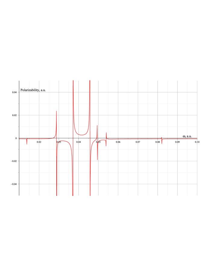
We consider differential dynamic polarizability in the M1 transition between first and second excited states of Sm¹⁴⁺. These states are shown in Table 2 in bold. Both states are very long-living states. Although, there is an allowed E1 transition from second exited state to the ground state we expect it to be very weak for reasons discussed above (see also calculated E1-transition amplitudes in Table 1). The first excited state can decay to the ground state only via E3 transition. Due to its high order and small frequency the probability of the transition is extremely small.

Figure 1 presents results of calculation of differential polarizability of M1 transition between first and second exited states in Sm⁺¹⁴ (reference transition). Energy levels within the optical range which contribute to the polarizability of the reference transition are listed in Table 1.

Table 3: Energy levels of Sm¹⁴⁺ recovered from data on Fig. 2. $\Delta E$ and $A$ are the interpolation parameters in eq. (13). Sign of $A$ together with theoretical calculation results allows to pick correct one (bold) of two possible values of $E_{k}$ - exited energy level, that contributes to reference transition differential polarizability.

$\Delta E$, a.u.	$A/2(3J+1),a_{0}^{2}$	$\left<i||E1||f\right>^{2},a_{0}^{2}$	$E_{k}$, cm-1
0.0139	$+9.07\times 10^{-7}$	$9.02\times 10^{-7}$	3053-3052=1
			1243+3052=4295
0.0288	$-4.34\times 10^{-5}$	$4.36\times 10^{-5}$	3053+6324=9377
			1243-6324=-5081
0.0371	$+1.22\times 10^{-4}$	$1.21\times 10^{-4}$	1243+8146=9389
			3053-8146=-5093
0.0456	$-1.39\times 10^{-4}$	$1.44\times 10^{-4}$	3053+10013=13066
			1243-10013=-8830
0.0494	$-1.52\times 10^{-5}$	$1.50\times 10^{-5}$	3053+10847=13900
			1243-10847=-9604
0.0539	$+4.43\times 10^{-6}$	$4.41\times 10^{-6}$	1243+11835=13078
			3053-11835=-8782
0.0820	$-2.03\times 10^{-6}$	$1.96\times 10^{-6}$	3053+18005=21058
			1243-18005=-16762

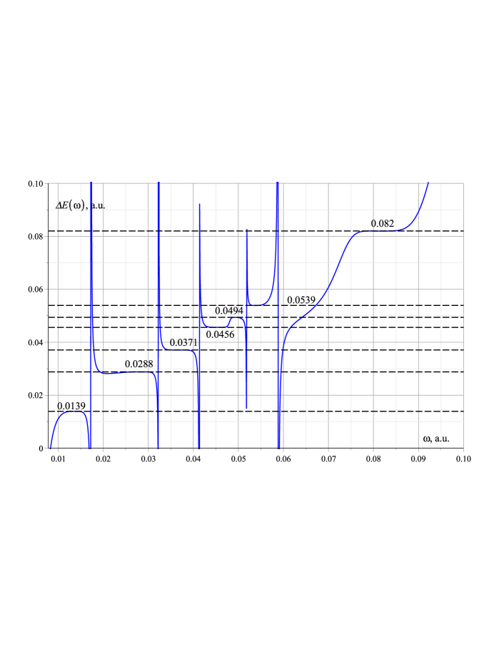
The results for relative position of the levels given by equation (14) are presented on Fig. 2. Presence of horizontal regions (same value of $\Delta E$ for different values of $\omega$) indicates the existence of frequency intervals where one resonance strongly dominates. Fitting of the dynamic polarizability using (14) in these frequency intervals recovers the positions of the energy levels which are in good agreement with direct calculations. This means that such approximation for differential polarizability is valid near resonances. The frequency intervals in which level can be detected now are of the order of $10^{-4}$ a.u.

There is an additional uncertainty in fitting procedure which needs to be discussed. When differential polarizability is considered and energy distance to the resonance $\Delta E$ is found from the fitting procedure, it is not known to energy of which of two states this $\Delta E$ should be added to find the position of the resonance level. There is also a question about the sign of $\Delta E$. The sign is always positive for the ground state polarizability. For differential polarizability of excited states the sign of $\Delta E$ must be consistent with the sign of $A$ (see (14)). This is evident from comparing (12) and (13). If $A<0$ then the energy of the resonance state is either $E_{e}+\Delta E$ or $E_{g}-\Delta E$. If $A>0$ then the energy is $E_{e}-\Delta E$ or $E_{g}+\Delta E$. The actual choice between these two possibilities is easy when calculated spectrum is available. Note that the accuracy of the calculations does not have to be very high since we only need to choose between two very distinct possibilities.

Table 3 illustrates reconstruction of the energy levels of Sm¹⁴⁺ from the data on the dynamic scalar polarizability of the M1 transition (Fig. 1). First two columns presents the values of $\Delta E$ and $A$ obtained from (14) using the values of the polarizabilities close to corresponding resonance. The last column of the table shows the recovering of the energies of the resonance states using presumably known energies of the states for which polarizability is measured and $\Delta E$ from first column. The right choice of the sign of $\Delta E$ and to the energy of which of the two states it should be added is shown in bold. The resulting energies agree well with calculated energies of Table 2. Note that the energies of the states which contribute to polarizabilities of both considered states are found twice.

Third column in Table 3 presents the squared reduced matrix element of the electric dipole transition which can be compared with the parameter $A$. In a single-resonance approximation they are related by $|A|=\langle g||E1||e\rangle^{2}/2(3J+1)$. One can see from the table that they are really close in value. Some small difference illustrates the accuracy of fitting by (13). The data in Table 3 shows that in the frequency intervals where the fitting formula (13) works well it can be used to recover not only the energy positions of the resonance states but also the values of electric dipole transition amplitudes.

The procedure considered above implies dynamic Stark shift of reference transition energy in external electric field of a laser. This shift is suppressed due to small values of electric dipole transition amplitudes. The amplitudes are small because the transitions cannot go between leading configurations and appear only due to configuration mixing. On the other hand, there are magnetic dipole transitions which are not suppressed because they go between states of the same configuration. In this situation magnetic dipole transitions can give significant contribution to the dynamic polarizability. To check this we have performed calculations of the M1 amplitudes for transitions which may affect the energy shift of the reference transition. The results are presented in lower lines of Table 1. To present M1 amplitudes we use the relation Bohr magneton $\mu_{B}=\alpha/2\approx 3.65\times 10^{-3}$ a.u. As one can notice the values of M1 and E1 amplitudes are of the same order of magnitude. Therefore, they should be included in the calculation of the total energy shift. The shift is described by the same equations as ones presented in Appendix after replacing electric field with magnetic in (10) and E1 with M1 amplitudes in (11). The analysis based on formula (13) is still the same. There are going to be extra peaks on the graph of the energy shift as a function of external frequency. This complicates the analysis, however the positive side of this is that it allows to see more levels. Theoretical calculations might be used to help identify the states where the resonances originate from.

The same relation between optical E1 and M1 transitions is expected to be valid for many HCI with more than one valence electron. In such systems electric dipole transition amplitudes are small because they cannot go between leading configurations and appear only due to configuration mixing. On the other hand, there are always states of the same configuration where M1 amplitudes are of the order of Borh magneton.

Table 4 presents the results of similar calculations for the Sm¹³⁺ ion. This ion has one extra electron above closed shells which leads to much larger number of transitions within the optical range. The reference transition is the M1 transition between the ground and first exited states with the energy of 6787 cm^-1. The last column of the table represents the amplitudes, that can be used to reduce the number of fitting parameters.

For this ion there are only two levels of odd parity (reference transition) within optical range. Therefore for the Sm¹³⁺ ion there will be no extra resonances in energy shift due to laser magnetic field as it was for the Sm¹⁴⁺ ion.

Table 4: E1-allowed transitions within the optical wave-lengths from one of the reference levels of Sm¹³⁺.

initial state		final state		transition	matrix
$5s^{2}4f^{1}$, odd		$5s^{1}4f^{2}$, even		energy,	element
$J_{i}$	$E_{i},$cm-1	$J_{f}$	$E_{f},$cm-1	a.u.	$\left<i||E1||f\right>,a_{0}$
2.5	0	1.5	31974	0.1457	$-3.5\times 10^{-5}$
2.5	0	1.5	59831	0.2726	$-7.9\times 10^{-3}$
2.5	0	1.5	63794	0.2907	$-3.4\times 10^{-3}$
2.5	0	2.5	33648	0.1533	$-3.2\times 10^{-3}$
2.5	0	2.5	47679	0.2172	$-1.4\times 10^{-2}$
2.5	0	2.5	59004	0.2688	$-5.9\times 10^{-4}$
2.5	0	3.5	22824	0.1040	$-2.1\times 10^{-3}$
2.5	0	3.5	35940	0.1638	$3.0\times 10^{-3}$
2.5	0	3.5	44036	0.2006	$1.1\times 10^{-2}$
2.5	0	3.5	53901	0.2456	$2.3\times 10^{-3}$
3.5	6787	2.5	33648	0.1224	$0.3\times 10^{-3}$
3.5	6787	2.5	47679	0.1863	$-2.5\times 10^{-3}$
3.5	6787	2.5	59004	0.2379	$6.8\times 10^{-3}$
3.5	6787	3.5	22824	0.0731	$0.3\times 10^{-3}$
3.5	6787	3.5	35940	0.1328	$2.0\times 10^{-3}$
3.5	6787	3.5	44036	0.1697	$-6.9\times 10^{-3}$
3.5	6787	3.5	53901	0.2147	$1.4\times 10^{-2}$
3.5	6787	4.5	25357	0.0846	$-3.0\times 10^{-3}$
3.5	6787	4.5	37041	0.1378	$1.2\times 10^{-2}$
3.5	6787	4.5	39687	0.1499	$3.0\times 10^{-4}$
3.5	6787	4.5	46921	0.1829	$1.7\times 10^{-2}$

IV Conclusions

It has been shown that the analysis of the dynamic Stark shift for a single transition in HCI can be used to recover a significant part of the spectrum of this ion as well as the values of the electric dipole transition amplitudes between the shifted states and states which contribute to their polarizabilities. Highly charged ions Sm¹⁴⁺ and Sm¹³⁺ considered in the paper are of particular interest since they are candidates for atomic clocks and for the search for time variation of the fine structure constant. The ions have relatively simple electron structure with two and three valence electrons above closed shells. This makes it easier to base the analysis on the theoretical calculations of the polarizabilities. However, similar analysis based on experimental data is not limited to ions with simple electron structure and can be useful for experimental study of wide range of the HCI.

Appendix A Stark shift near resonance

Energy shift of atomic levels in the presence of external electric field $\mathcal{E}$ of linearly polarized light with frequency $\omega$ can be written as Manakov:1986 ; Manakov:1978

$$\Delta\varepsilon_{nJM}=-\left[\alpha_{nJ}^{S}(\omega)+\alpha_{nJ}^{T}(\omega)\frac{3M^{2}-J(J+1)}{J(2J-1)}\right]\frac{\mathcal{E}^{2}}{4},$$ (10)

where $n,J,M$ are main quantum number, total electron angular momentum and its projection respectively and $\alpha_{nf}^{S}(\omega)$ and $\alpha_{nf}^{T}(\omega)$ are scalar and tensor dynamic polarizabilities of the state $n,J$. Averaging over all total angular momentum projections cancels out tensor polarizability, therefore for simplicity we will consider only scalar polarizability. It can be written as

$$\alpha_{nJ}^{S}(\omega)=\frac{2}{3(2J+1)}\sum_{n^{\prime},J^{\prime}=J-1}^{J^{\prime}=J+1}\frac{\Delta E\langle nJ||\textbf{d}||n^{\prime}J^{\prime}\rangle^{2}}{\Delta E^{2}-\omega^{2}},$$ (11)

where $\Delta E=E_{n}-E_{n^{\prime}}$, $\textbf{d}=-e\textbf{r}$ is the electric dipole operator and summation goes over complete set of intermediate states. The above equation has singular points at $\omega=E_{n}-E_{n^{\prime}}$, which correspond to the resonances. If frequency $\omega$ of the laser light is close to a resonance it is convenient to rewrite 11 in the following form

$$\begin{split}&\alpha_{nJ}^{S}(\omega)=-\frac{2}{3(2J+1)}\left(\frac{1}{2}\frac{\langle nJ||\textbf{d}||kJ^{\prime}\rangle^{2}}{(E_{n}-E_{k})-\omega}+\right.\\ &\frac{1}{2}\frac{\langle nJ||\textbf{d}||kJ^{\prime}\rangle^{2}}{(E_{n}-E_{k})+\omega}+\left.\sum_{n^{\prime}\neq k}\frac{(E_{n}-E_{n^{\prime}})\langle nJ||\textbf{d}||n^{\prime}J^{\prime}\rangle^{2}}{(E_{n}-E_{n^{\prime}})^{2}-\omega^{2}}\right).\end{split}$$ (12)

Since $\omega$ is close to resonance energy $\Delta E=|E_{n}-E_{k}|$ first or second term in brackets determines behavior of $\alpha_{0}(\omega)$ depending on the sign of $\Delta E$. Hence for differential polarizability $\alpha^{S}(\omega)=\alpha_{n_{1}J_{1}}^{S}(\omega)-\alpha_{n_{2}J_{2}}^{S}(\omega)$ of the reference transition near resonance a simple analytical formula containing single resonance term and some simple approximation for the rest of the sum can be employed:

$$\Delta\alpha_{nJ}^{S}(\omega)=-\left(\frac{A}{\Delta E-\omega}+K\omega+C\right).$$ (13)

Here $nJ$ is the one of the two states $n_{1}J_{1}$ or $n_{2}J_{2}$ which satisfy the resonance condition $\omega\approx|E_{n^{\prime}J^{\prime}}-E_{nJ}|$; $A$, $K$, $C$ and $\Delta E$ are fitting parameters. It is assumed that $\Delta E>0$. Comparing (13) to (11) one can see that the parameter $A$ is related to the electric dipole transition amplitude between the resonance states $nJ$ and $n^{\prime}J^{\prime}$ by $A=\pm\langle nJ||\textbf{d}||n^{\prime}J^{\prime}\rangle^{2}/3(2J+1)$. The plus sign corresponds to the case when $E_{n^{\prime}J^{\prime}}>E_{nJ}$, the minus sign is when $E_{n^{\prime}J^{\prime}}<E_{nJ}$. Fitting measured differential Stark shift of the frequency of the reference transition as a function of the laser frequency using (13) allows one to find the position of the resonance ($\Delta E$) and the value of the electric dipole transition amplitude between the states involved in the resonance ($A$). Note that there is still uncertainty due to the fact that it is still not known which of the the two reference states $n_{1}J_{1}$ or $n_{2}J_{2}$ is involved in the resonance. Fitting by (13) does not distinguish between the two possibilities. One has to compare with the calculations or use some other considerations. For example, if $A<0$ then the state $nJ$ cannot be the ground state. More generally, it cannot be the state from which there is no electric dipole transitions to the lower states.

It can be useful to have the formulae for the parameters $\Delta E$, $A$, $K$ and $C$ in (13) for the case when the differential polarizability is known at four values of laser frequency, $\omega_{1},\omega_{2},\omega_{3}$ and $\omega_{4}$ separated by equal frequency intervals $\Delta\omega$. The formulae are

$$\Delta E = \frac{\omega_{4}-Q\omega_{1}}{1-Q},$$ (14)

$$Q = \frac{\alpha_{nJ}^{S}(\omega_{1})-2\alpha_{nJ}^{S}(\omega_{2})+\alpha_{nJ}^{S}(\omega_{3})}{\alpha_{nJ}^{S}(\omega_{2})-2\alpha_{nJ}^{S}(\omega_{3})+\alpha_{nJ}^{S}(\omega_{4})}$$

$$A = -\frac{\alpha_{nJ}^{S}(\omega_{1})-2\alpha_{nJ}^{S}(\omega_{2})+\alpha_{nJ}^{S}(\omega_{3})}{\Delta\omega^{2}}\frac{3(2J+1)}{4}\times$$

$$(\Delta E-\omega_{1})(\Delta E-\omega_{2})(\Delta E-\omega_{3}).$$

Figure 1: Difference of the scalar polarizabilities (11) for Sm⁺¹⁴ M1 transition. The resonances appear for $\omega$ equal to 0.0139; 0.0288; 0.0371; 0.0456; 0.0494; 0.0539; 0.0820.

Figure 2: Energy level position $\Delta E$ given by (14) relative to one of the reference transition levels, as a function of external laser frequency $\omega_{1}$. Dashed lines corresponds to resonances in polarizability presented in Fig. 1. For small values of $\Delta\omega$ there is no sensitivity to $\Delta\omega$.

References

- (1) A. Derevianko, V.A. Dzuba, and V. V. Flambaum, Phys. Rev. Lett. 109, 180801 (2012).
- (2) V. A. Dzuba, A. Derevianko, and V. V. Flambaum, Phys. Rev. A 86, 054501 (2012); Phys. Rev. A 87, 029906(E) (2013).
- (3) J. C. Berengut, V. A. Dzuba, V. V. Flambaum, Phys. Rev. Lett. 105, 120801 (2010).
- (4) J. C. Berengut, V. A. Dzuba, V. V. Flambaum, and A. Ong, Phys. Rev. Lett. 106, 210802 (2011).
- (5) J. C. Berengut, V. A. Dzuba, V. V. Flambaum, A. Ong, Phys. Rev. Lett. 109, 070802 (2012).
- (6) V. A. Dzuba, A. Derevianko, and V. V. Flambaum, Phys. Rev. A 86, 054502 (2012).
- (7) J. C. Berengut, V. A. Dzuba, V. V. Flambaum, A. Ong, Phys. Rev. A 86, 022517 (2012).
- (8) M. S. Safronova et al, to be published.
- (9) V. A. Dzuba, V. V. Flambaum, and M. G. Kozlov, Phys. Rev. A 54, 3948 (1996).
- (10) V. A. Dzuba, Phys. Rev. A 71, 032512 (2005).
- (11) V. A. Dzuba and J. S. M. Ginges, Phys. Rev. A 73, 032503 (2006).
- (12) V. A. Dzuba, V. V. Flambaum, and M. G. Kozlov, Phys. Rev. A, 54, 3948 (1996); JETP Letteres, 63, 882 (1996).
- (13) V. A. Dzuba, V. V. Flambaum, P. G. Silvestrov, O. P. Sushkov, J. Phys. B 20, 1399 (1987).
- (14) A. Derevianko, W. R. Johnson, M. S. Safronova, J. F. Babb, Phys. Rev. Lett. 82, 3589 (1999).
- (15) V. A. Dzuba and A. Derevianko, J. Phys. B 43, 074011 (2010).
- (16) A. Dalgarno and J. T. Lewis, Proc. R. Soc. Lond. A 223, 70 (1955).
- (17) W. R. Johnson, Adv. At. Mol. Opt. Phys. 25, 375 (1988).
- (18) N. L. Manakov, V. D. Ovsiannikov, L. P. Rapoport, Phys. Rep. 141, 320 (1986).
- (19) N. L. Manakov, V. D. Ovsiannikov, Phys. Rep. 75, 803 (1978).
- (20) V. A. Dzuba, V. V. Flambaum, P. G. Silvestrov, O. P. Sushkov, J. Phys. B 20, 1399-1412 (1987).
- (21) V. A. Dzuba, J. S. M. Ginges, Phys. Rev. A, 73 032503 (2006).
- (22) V. A. Dzuba and V. V. Flambaum, J. Phys. B 40 227 (2007).
- (23) H. Karlsson, U. Litzén, Phys. Scr. 60, 321 (1999).