Minimizing Finite Sums with the Stochastic Average Gradient
Abstract
We analyze the stochastic average gradient (SAG) method for optimizing the sum of a finite number of smooth convex functions. Like stochastic gradient (SG) methods, the SAG method’s iteration cost is independent of the number of terms in the sum. However, by incorporating a memory of previous gradient values the SAG method achieves a faster convergence rate than black-box SG methods. The convergence rate is improved from to in general, and when the sum is strongly-convex the convergence rate is improved from the sub-linear to a linear convergence rate of the form for . Further, in many cases the convergence rate of the new method is also faster than black-box deterministic gradient methods, in terms of the number of gradient evaluations. This extends our earlier work [Le Roux et al., 2012], which only lead to a faster rate for well-conditioned strongly-convex problems. Numerical experiments indicate that the new algorithm often dramatically outperforms existing SG and deterministic gradient methods, and that the performance may be further improved through the use of non-uniform sampling strategies.
1 Introduction
A plethora of the optimization problems arising in practice involve computing a minimizer of a finite sum of functions measuring misfit over a large number of data points. A classical example is least-squares regression,
where the and are the data samples associated with a regression problem. Another important example is logistic regression,
where the and are the data samples associated with a binary classification problem. A key challenge arising in modern applications is that the number of data points (also known as training examples) can be extremely large, while there is often a large amount of redundancy between examples. The most wildly successful class of algorithms for taking advantage of the sum structure for problems where is very large are stochastic gradient (SG) methods [Robbins and Monro, 1951, Bottou and LeCun, 2003]. Although the theory behind SG methods allows them to be applied more generally, SG methods are often used to solve the problem of optimizing a finite sample average,
| (1) |
In this work, we focus on such finite data problems where each is smooth and convex.
In addition to this basic setting, we will also be interested in cases where the sum has the additional property that it is strongly-convex. This often arises due to the use of a strongly-convex regularizer such as the squared -norm, resulting in problems of the form
| (2) |
where each is a data-misfit function (as in least-squares and logistic regression) and the positive scalar controls the strength of the regularization. These problems can be put in the framework of (1) by using the choice
The resulting function will be strongly-convex provided that the individual loss functions are convex. An extensive list of convex loss functions used in a statistical data-fitting context is given by Teo et al. [2007], and non-smooth loss functions (or regularizers) can also be put in this framework by using smooth approximations (for example, see Nesterov [2005]).
For optimizing problem (1), the standard deterministic or full gradient (FG) method, which dates back to Cauchy [1847], uses iterations of the form
| (3) |
where is the step size on iteration . Assuming that a minimizer exists, then under standard assumptions the sub-optimality achieved on iteration of the FG method with a constant step size is given by
when is convex [see Nesterov, 2004, Corollary 2.1.2]. This results in a sublinear convergence rate. When is strongly-convex, the error also satisfies
for some which depends on the condition number of [see Nesterov, 2004, Theorem 2.1.5]. This results in a linear convergence rate, which is also known as a geometric or exponential rate because the error is cut by a fixed fraction on each iteration. Unfortunately, the FG method can be unappealing when is large because its iteration cost scales linearly in .
The main appeal of SG methods is that they have an iteration cost which is independent of , making them suited for modern problems where may be very large. The basic SG method for optimizing (1) uses iterations of the form
| (4) |
where at each iteration an index is sampled uniformly from the set . The randomly chosen gradient yields an unbiased estimate of the true gradient and one can show under standard assumptions (see [Nemirovski et al., 2009]) that, for a suitably chosen decreasing step-size sequence , the SG iterations have an expected sub-optimality for convex objectives of
and an expected sub-optimality for strongly-convex objectives of
In these rates, the expectations are taken with respect to the selection of the variables. These sublinear rates are slower than the corresponding rates for the FG method, and under certain assumptions these convergence rates are optimal in a model of computation where the algorithm only accesses the function through unbiased measurements of its objective and gradient (see Nemirovski and Yudin [1983], Nemirovski et al. [2009], Agarwal et al. [2012]). Thus, we should not expect to be able to obtain the convergence rates of the FG method if the algorithm only relies on unbiased gradient measurements. Nevertheless, by using the stronger assumption that the functions are sampled from a finite dataset, in this paper we show that we can achieve the convergence rates of FG methods while preserving the iteration complexity of SG methods.
The primary contribution of this work is the analysis of a new algorithm that we call the stochastic average gradient (SAG) method, a randomized variant of the incremental aggregated gradient (IAG) method of Blatt et al. [2007]. The SAG method has the low iteration cost of SG methods, but achieves the convergence rates stated above for the FG method. The SAG iterations take the form
| (5) |
where at each iteration a random index is selected and we set
| (6) |
That is, like the FG method, the step incorporates a gradient with respect to each function. But, like the SG method, each iteration only computes the gradient with respect to a single example and the cost of the iterations is independent of . Despite the low cost of the SAG iterations, we show in this paper that with a constant step-size the SAG iterations have an convergence rate for convex objectives and a linear convergence rate for strongly-convex objectives, like the FG method. That is, by having access to and by keeping a memory of the most recent gradient value computed for each index , this iteration achieves a faster convergence rate than is possible for standard SG methods. Further, in terms of effective passes through the data, we will also see that for many problems the convergence rate of the SAG method is also faster than is possible for standard FG methods.
One of the main contexts where minimizing the sum of smooth convex functions arises is machine learning. In this context, is often an empirical risk (or a regularized empirical risk), which is a sample average approximation to the true risk that we are interested in. It is known that with training examples the empirical risk minimizer (ERM) has an error for the true risk of in the convex case and in the strongly-convex case. Since these rates are achieved by doing one pass through the data with an SG method, in the worst case the SAG algorithm applied to the empirical risk cannot improve the convergence rate in terms of the true risk over this simple method. Nevertheless, Srebro and Sridharan [2011] note that “overwhelming empirical evidence shows that for almost all actual data, the ERM is better. However, we have no understanding of why this happens”. Although our analysis does not give insight into the better performance of ERM, our analysis shows that the SAG algorithm will be preferable to SG methods for finding the ERM and hence for many machine learning applications.
The next section reviews several closely-related algorithms from the literature, including previous attempts to combine the appealing aspects of FG and SG methods. However, despite years of extensive research on SG methods, with a significant portion of the applications focusing on finite datasets, we believe that this is the first general method that achieves the convergence rates of FG methods while preserving the iteration cost of standard SG methods. Section 3 states the (standard) assumptions underlying our analysis and gives our convergence rate results. Section 4 discusses practical implementation issues including how we adaptively set the step size and how we can reduce the storage cost needed by the algorithm. For example, we can reduce the memory requirements from to in the common scenario where each only depends on a linear function of , as in least-squares and logistic regression. Section 5 presents a numerical comparison of an implementation based on SAG to competitive SG and FG methods, indicating that the method may be very useful for problems where we can only afford to do a few passes through a data set.
A preliminary conference version of this work appears in Le Roux et al. [2012], and we extend this work in various ways. Most notably, the analysis in the prior work focuses only on showing linear convergence rates in the strongly-convex case while the present work also gives an convergence rate for the general convex case. In the prior work we show (Proposition 1) that a small step-size gives a slow linear convergence rate (comparable to the rate of FG methods in terms of effective passes through the data), while we also show (Proposition 2) that a much larger step-size yields a much faster convergence rate, but this requires that is sufficiently large compared to the condition number of the problem. In the present work (Section 3) our analysis yields a very fast convergence rate using a large step-size (Theorem 1), even when this condition required by the prior work is not satisfied. Surprisingly, for ill-conditioned problems our new analysis shows that using SAG iterations can be nearly times as fast as the standard gradient method. To prove this stronger result, Theorem 1 employs a Lyapunov function that generalizes the Lyapunov functions used in Propositions 1 and 2 of the previous work. This new Lyapunov function leads to a unified proof for both the convex and the strongly-convex cases, and for both well-conditioned and ill-conditioned problems. However, this more general Lyapunov function leads to a more complicated analysis. To significantly simplify the formal proof, we use a computed-aided strategy to verify the non-negativity of certain polynomials that arise in the proof. Beyond this significantly strengthened result, in this work we also argue that yet-faster convergence rates may be achieved by non-uniform sampling (Section 4.8) and present numerical results showing that this can lead to drastically improved performance (Section 5.5).
2 Related Work
There are a large variety of approaches available to accelerate the convergence of SG methods, and a full review of this immense literature would be outside the scope of this work. Below, we comment on the relationships between the new method and several of the most closely-related ideas.
Momentum: SG methods that incorporate a momentum term use iterations of the form
see Tseng [1998]. It is common to set all for some constant , and in this case we can rewrite the SG with momentum method as
We can re-write the SAG updates (5) in a similar form as
| (7) |
where the selection function is equal to if is the maximum iteration number where example was selected and is set to otherwise. Thus, momentum uses a geometric weighting of previous gradients while the SAG iterations select and average the most recent evaluation of each previous gradient. While momentum can lead to improved practical performance, it still requires the use of a decreasing sequence of step sizes and is not known to lead to a faster convergence rate.
Gradient Averaging: Closely related to momentum is using the sample average of all previous gradients,
which is similar to the SAG iteration in the form (5) but where all previous gradients are used. This approach is used in the dual averaging method of Nesterov [2009] and, while this averaging procedure and its variants lead to convergence for a constant step size and can improve the constants in the convergence rate [Xiao, 2010], it does not improve on the sublinear convergence rates for SG methods.
Iterate Averaging: Rather than averaging the gradients, some authors propose to perform the basic SG iteration but use an average over certain values as the final estimator. With a suitable choice of step-sizes, this gives the same asymptotic efficiency as Newton-like second-order SG methods and also leads to increased robustness of the convergence rate to the exact sequence of step sizes [Polyak and Juditsky, 1992, Bach and Moulines, 2011]. Bather’s method [Kushner and Yin, 2003, §1.3.4] combines gradient averaging with online iterate averaging and also displays appealing asymptotic properties. Several authors have recently shown that suitable iterate averaging schemes obtain an rate for strongly-convex optimization even for non-smooth objectives [Hazan and Kale, 2011, Rakhlin et al., 2012]. However, none of these methods improve on the and rates for SG methods.
Stochastic versions of FG methods: Various options are available to accelerate the convergence of the FG method for smooth functions, such as the accelerated full gradient (AFG) method of Nesterov [1983], as well as classical techniques based on quadratic approximations such as diagonally-scaled FG methods, non-linear conjugate gradient, quasi-Newton, and Hessian-free Newton methods (see [Nocedal and Wright, 2006]). There has been a substantial amount of work on developing stochastic variants of these algorithms, with several of the notable recent examples including Bordes et al. [2009], Hu et al. [2009], Sunehag et al. [2009], Ghadimi and Lan [2010], Martens [2010], Xiao [2010]. Duchi et al. [2011] have recently shown an improved regret bound using a diagonal scaling that takes into account previous gradient magnitudes. Alternately, if we split the convergence rate into a deterministic and stochastic part, these methods can improve the dependency of the convergence rate of the deterministic part [Hu et al., 2009, Ghadimi and Lan, 2010, Xiao, 2010]. However, we are not aware of any existing method of this flavor that improves on the and dependencies on the stochastic part. Further, many of these methods typically require carefully setting parameters (beyond the step size) and often aren’t able to take advantage of sparsity in the gradients .
Constant step size: If the SG iterations are used for strongly-convex optimization with a constant step size (rather than a decreasing sequence), then Nedic and Bertsekas [2000, Proposition 3.4] showed that the convergence rate of the method can be split into two parts. The first part depends on and converges linearly to . The second part is independent of and does not converge to . Thus, with a constant step size, the SG iterations have a linear convergence rate up to some tolerance, and in general after this point the iterations do not make further progress. Indeed, up until the recent work of Bach and Moulines [2013], convergence of the basic SG method with a constant step size had only been shown for the strongly-convex quadratic case (with averaging of the iterates) [Polyak and Juditsky, 1992], or under extremely strong assumptions about the relationship between the functions [Solodov, 1998]. This contrasts with the method we present in this work which converges to the optimal solution using a constant step size and does so with a linear rate (without additional assumptions).
Accelerated methods: Accelerated SG methods, which despite their name are not related to the aforementioned AFG method, take advantage of the fast convergence rate of SG methods with a constant step size. In particular, accelerated SG methods use a constant step size by default, and only decrease the step size on iterations where the inner-product between successive gradient estimates is negative [Kesten, 1958, Delyon and Juditsky, 1993]. This leads to convergence of the method and allows it to potentially achieve periods of faster convergence where the step size stays constant. However, the overall convergence rate of the method is not improved.
Hybrid Methods: Some authors have proposed variants of the SG method for problems of the form (1) that seek to gradually transform the iterates into the FG method in order to achieve a faster convergence rate. Bertsekas [1997] proposes to go through the data cyclically with a specialized weighting that allows the method to achieve a linear convergence rate for strongly-convex quadratic functions. However, the weighting is numerically unstable and the linear convergence rate presented treats full passes through the data as iterations. A related strategy is to group the functions into ‘batches’ of increasing size and perform SG iterations on the batches. Friedlander and Schmidt [2012] give conditions under which this strategy achieves the and convergence rates of FG methods. However, in both cases the iterations that achieve the faster rates have a cost that is not independent of , as opposed to SAG iterations.
Incremental Aggregated Gradient: Blatt et al. [2007] present the most closely-related algorithm to the SAG algorithm, the IAG method. This method is identical to the SAG iteration (5), but uses a cyclic choice of rather than sampling the values. This distinction has several important consequences. In particular, Blatt et al. are only able to show that the convergence rate is linear for strongly-convex quadratic functions (without deriving an explicit rate), and their analysis treats full passes through the data as iterations. Using a non-trivial extension of their analysis and a novel proof technique involving bounding the gradient and iterates simultaneously by a Lyapunov potential function, in this work we give an rate for general convex functions and an explicit linear convergence rate for general strongly-convex functions using the SAG iterations that only examine a single function. Further, as our analysis and experiments show, the SAG iterations allow a much larger step size than is required for convergence of the IAG method. This leads to more robustness to the selection of the step size and also, if suitably chosen, leads to a faster convergence rate and substantially improved practical performance. This shows that the simple change (random selection vs. cycling) can dramatically improve optimization performance.
Special Problem Classes: For certain highly-restricted classes of problems, it is possible to show faster convergence rates for methods that only operate on a single function . For example, Strohmer and Vershynin [2009] show that the randomized Kaczmarz method with a particular sampling scheme achieves a linear convergence rate for the problem of solving consistent linear systems. It is also known that the SG method with a constant step-size has the and convergence rates of FG methods if is bounded by a linear function of for all and Schmidt and Le Roux [2013]. This is the strong condition required by Solodov [1998] to show convergence of the SG method with a constant step size. Unlike these previous works, our analysis in the next section applies to general that satisfy standard assumptions, and only requires gradient evaluations of the functions rather than dual block-coordinate steps.
Subsequent work: Since the first version of this work was released, there has been an explosion of research into stochastic gradient methods with faster convergence rates. It has been shown that similar rates can be achieved for certain constrained and non-smooth problems, that similar rates can be achieved without the memory requirements, that Newton-like variants of the method may be possible, and that similar rates can be achieved with other algorithms. In Section 6, we survey these recent developments.
3 Convergence Analysis
In our analysis we assume that each function in (1) is convex and differentiable, and that each gradient is Lipschitz-continuous with constant , meaning that for all and in and each we have
| (8) |
This is a fairly weak assumption on the functions, and in cases where the are twice-differentiable it is equivalent to saying that the eigenvalues of the Hessians of each are bounded above by . We will also assume the existence of at least one minimizer that achieves the optimal function value. We denote the average iterate by , and the variance of the gradient norms at the optimum by . Our convergence results consider two different initializations for the variables: setting for all , or setting them to the centered gradient at the initial point given by . We note that all our convergence results are expressed in terms of expectations with respect to the internal randomization of the algorithm (the selection of the random variables ), and not with respect to the data which is assumed to be deterministic and fixed.
In addition to this basic convex case discussed above, we will also consider the case where the average function is strongly-convex with constant , meaning that the function is convex. For twice-differentiable , this is equivalent to requiring that the eigenvalues of the Hessian of are bounded below by . This is a stronger assumption that is often not satisfied in practical applications. Nevertheless, in many applications we are free to choose a regularizer of the parameters, and thus we can add an -regularization term as in (2) to transform any convex problem into a strongly-convex problem (in this case we have ). Note that strong-convexity implies the existence of a unique that achieves the optimal function value.
Under these standard assumptions, we now state our convergence result.
Theorem 1.
With a constant step size of , the SAG iterations satisfy for :
where if we initialize with we have
and if we initialize with we have
Further, if is -strongly convex we have
The proof is given in Appendix B of the extended version of this paper, and involves finding a Lyapunov function for a non-linear stochastic dynamical system defined on the and variables that converges to zero at the above rates, and showing that this function dominates the expected sub-optimality . This is the same approach used to show Proposition 1 and 2 in the conference version of the paper [Le Roux et al., 2012], but in this work we use a more general Lyapunov function that gives a much faster rate for ill-conditioned problems and also allows us to analyze problems that are not strongly-convex. To simplify the analysis of this more complicated Lyapunov function, our new proof verifies positivity of certain polynomials that arise in the bound using a computer-aided approach.
Note that while the first part of Theorem (1) is stated for the average , with a trivial change to the proof technique it can be shown to also hold for any iterate where is lower than the average function value up to iteration , . Thus, in addition to the result also holds for the best iterate. We also note that our bounds are valid for any greater than or equal to the minimum satisfying (8), implying an and linear convergence rate for any (but the bound becomes worse as grows). Although initializing each with the centered gradient may have an additional cost and slightly worsens the dependency on the initial sub-optimality , it removes the dependency on the variance of the gradients at the optimum. While we have stated Theorem 1 in terms of the function values, in the strongly-convex case we also obtain a convergence rate on the iterates because we have
Theorem 1 shows that the SAG iterations are advantageous over SG methods in later iterations because they obtain a faster convergence rate. However, the SAG iterations have a worse constant factor because of the dependence on . We can improve the dependence on using an appropriate choice of . In particular, following Le Roux et al. [2012] we can set to the result of iterations of an appropriate SG method. In this setting, the expectation of is in the convex setting, while both and would be in in the strongly-convex setting. If we use this initialization of and set , then in terms of and the SAG convergence rates take the form and in the convex and strongly-convex settings, instead of the and rates implied by Theorem 1. However, in our experiments we do not use an SG initialization but rather use a minor variant of SAG in the early iterations (discussed in the next section), which appears more difficult to analyze but which gives better empirical performance.
An interesting consequence of using a step-size of is that it makes the method adaptive to the strong-convexity constant . That is, for problems with a higher degree of local strong-convexity around the solution , the algorithm will automatically take advantage of this and yield a faster local rate. This can even lead to a local linear convergence rate if the problem is strongly-convex near the optimum but not globally strongly-convex. This adaptivity to the problem difficulty is in contrast to SG methods whose sequence of step sizes typically depend on global constants and thus do not adapt to local strong-convexity.
We have observed in practice that the IAG method with a step size of may diverge. While the step-size needed for convergence of the IAG iterations is not precisely characterized, we have observed that it requires a step-size of approximately in order to converge. Thus, the SAG iterations can tolerate a step size that is roughly times larger, which leads to increased robustness to the selection of the step size. Further, as our analysis and experiments indicate, the ability to use a large step size leads to improved performance of the SAG iterations. Note that using randomized selection with a larger step-size leading to vastly improved performance is not an unprecedented phenomenon; the analysis of Nedic and Bertsekas [2000] shows that the iterations of the basic stochastic gradient method with a constant step-size can achieve the same error bound as full cycles through the data of the cyclic variant of the method by using steps that are times larger (see the discussion after Proposition 3.4). Related results also appear in Collins et al. [2008], Lacoste-Julien et al. [2013] showing the advantage of stochastic optimization strategies over deterministic optimization strategies in the context of certain dual optimization problems.
The convergence rate of the SAG iterations in the strongly-convex case takes a somewhat surprising form. For ill-conditioned problems where , does not appear in the convergence rate and the SAG algorithm has nearly the same convergence rate as the FG method with a step size of , even though it uses iterations which are times cheaper. This indicates that the basic gradient method (under a slightly sub-optimal step-size) is not slowed down by using out-of-date gradient measurements for ill-conditioned problems. Although appears in the convergence rate in the well-conditioned setting where , if we perform iterations of SAG (i.e., one effective pass through the data), the error is multiplied by , which is independent of . Thus, in this setting each pass through the data reduces the excess objective by a constant multiplicative factor that is independent of the problem.
It is interesting to compare the convergence rate of SAG in the strongly-convex case with the known convergence rates for first-order methods [see Nesterov, 2004, §2]. In Table 1, we use two examples to compare the convergence rate of SAG to the convergence rates of the standard FG method, the faster AFG method, and the lower-bound for any first-order strategy (under certain dimensionality assumptions) for optimizing a function satisfying our assumptions. In this table, we compare the rate obtained for these FG methods to the rate obtained by running iterations of SAG, since this requires the same number of evaluations of . Case in this table focuses on a well-conditioned case where the rate of SAG is , while Case focuses on an ill-conditioned example where the rate is . Note that in the latter case the rate for the method may be faster.
In Table 1 we see that performing iterations of SAG can actually lead to a rate that is faster than the lower bound for FG methods. Thus, for certain problems SAG can be substantially faster than any FG method that does not use the structure of the problem. However, we note that the comparison is somewhat problematic because in the SAG rates is the Lipschitz constant of the functions, while in the FG method we only require that is an upper bound on the Lipschitz continuity of so it may be much smaller. To give a concrete example that takes this into account and also considers the rates of dual methods and coordinate-wise methods, in Appendix A of the extended version of this paper we attempt to more carefully compare the rates obtained for SAG with the rates of primal and dual FG and coordinate-wise methods for the special case of -regularized least-squares regression.
| Algorithm | Step Size | Theoretical Rate | Rate in Case 1 | Rate Case 2 |
|---|---|---|---|---|
| FG | ||||
| FG | ||||
| AFG | ||||
| Lower-Bound | — | |||
| SAG ( iters) |
4 Implementation Details
In Algorithm 1 we give pseudo-code for an implementation of the basic method, where we use a variable to track the quantity . This section focuses on further implementation details that are useful in practice. In particular, we discuss modifications that lead to better practical performance than the basic Algorithm 1, including ways to reduce the storage cost, how to handle regularization, how to set the step size, using mini-batches, and using non-uniform sampling. Note that an implementation of the algorithm that incorporates many of these aspects is available from the first author’s webpage.
4.1 Structured gradients and just-in-time parameter updates
For many problems the storage cost of for the vectors is prohibitive, but we can often use the structure of the gradients to reduce this cost. For example, a commonly-used specialization of (1) is linearly-parameterized models which take form
| (9) |
Since each is constant, for these problems we only need to store the scalar for rather than the full gradient . This reduces the storage cost from down to .
For problems where the vectors are sparse, an individual gradient will inherit the sparsity pattern of the corresponding . However, the update of in Algorithm 1 appears unappealing since in general will be dense, resulting in an iteration cost of . Nevertheless, we can take advantage of the simple form of the SAG updates to implement a ‘just-in-time’ variant of the SAG algorithm where the iteration cost is proportional to the number of non-zeroes in . In particular, we do this by not explicitly storing the full vector after each iteration. Instead, on each iteration we only compute the elements corresponding to non-zero elements of , by applying the sequence of updates to each variable since the last iteration where it was non-zero in . This sequence of updates can be applied efficiently since it simply involves changing the step size. For example, if variable has been zero in for iterations, then we can compute the needed value using
This update allows SAG to be efficiently applied to sparse data sets where and are both in the millions or higher but the number of non-zeros is much less than .
4.2 Re-weighting on early iterations
In the update of in Algorithm 1, we normalize the direction by the total number of data points . When initializing with we believe this leads to steps that are too small on early iterations of the algorithm where we have only seen a fraction of the data points, because many variables contributing to are set to the uninformative zero-vector. Following Blatt et al. [2007], the more logical normalization is to divide by , the number of data points that we have seen at least once (which converges to once we have seen the entire data set), leading to the update . Although this modified SAG method appears more difficult to analyze, in our experiments we found that running the basic SAG algorithm from the very beginning with this modification outperformed the basic SAG algorithm as well as the SG/SAG hybrid algorithm mentioned in the Section 3. In addition to using the gradient information collected during the first iterations, this modified SAG algorithm is also advantageous over hybrid SG/SAG algorithms because it only requires estimating a single constant step size.
4.3 Exact and efficient regularization
In the case of regularized objectives like (2), the cost of computing the gradient of the regularizer is independent of . Thus, we can use the exact gradient of the regularizer in the update of , and only use to approximate the sum of the functions. By incorporating the gradient of the regularizer explicitly, the update for in Algorithm 1 becomes , and in the case of -regularization the update for becomes
If the loss function gradients are sparse as in Section 4.1, then these modifications lead to a reduced storage requirement even though the gradient of the regularizer is dense. Further, although the update of again appears to require dense vector operations, we can implement the algorithm efficiently if the are sparse. In particular, to allow efficient multiplication of by the scalar , it is useful to represent in the form , where is a scalar and is a vector (as done by Shalev-Shwartz et al. [2011]). Under this representation, we can multiply by a scalar in by simply updating (though to prevent becoming too large or too small we may need to occasionally re-normalize by setting and ). To efficiently implement the vector subtraction operation, we can use a variant of the just-in-time updates from Section 4.1. In Algorithm 2, we give pseudo-code for a variant of SAG that includes all of these modifications, and thus uses no full-vector operations. This code uses a vector to keep track of the scalars , a vector to determine whether a data point has previously been visited, a vector to track the last time a variable was updated, and a vector to keep track of the cumulative sums needed to implement the just-in-time updates.
4.4 Warm starting
In many scenarios we may need to solve a set of closely-related optimization problems. For example, we may want to apply Algorithm 2 to a regularized objective of the form (2) for several values of the regularization parameter . Rather than solving these problems independently, we might expect to obtain better performance by warm-starting the algorithm. Although initializing with the solution of a related problem can improve performance, we can expect an even larger performance improvement if we also use the gradient information collected from a run of SAG for a close value of . For example, in Algorithm 2 we could initialize , , , , and based on a previous run of the SAG algorithm. In this scenario, Theorem 1 suggests that it may be beneficial in this setting to center the variables around .
4.5 Larger step sizes
In our experiments we have observed that utilizing a step size of , as in standard FG methods, always converged and often performed better than the step size of suggested by our analysis. Thus, in our experiments we used even though we do not have a formal analysis of the method under this step size. We also found that a step size of , which in the strongly-convex case corresponds to the best fixed step size for the FG method in the special case of [see Nesterov, 2004, Theorem 2.1.15], sometimes yields even better performance (though in other cases it performs poorly).
4.6 Line-search when is not known
In general the Lipschitz constant will not be known, but we may obtain a reasonable approximation of a valid by evaluating values while running the algorithm. In our experiments, we used a basic line-search where we start with an initial estimate , and double this estimate whenever we do not satisfy the inequality
which must be true if is valid. An important property of this test is that it depends on but not on , and thus the cost of performing this test is independent of . To avoid instability caused by comparing very small numbers, we only do this test when . Since is a global quantity but the algorithm will eventually remain within a neighbourhood of the optimal solution, it is possible that a smaller estimate of (and thus a larger step size) can be used as we approach . To potentially take advantage of this, we initialize with the slightly smaller at each iteration, so that the estimate of is halved if we do iterations (an effective pass through the data) and never violate the inequality. Note that in the case of -regularized objectives, we can perform the line-search to find an estimate of the Lipschitz constant of rather than , and then simply add to this value to take into account the effect of the regularizer.
Note that the cost of this line-search is independent of , making it suitable for large problems. Further, for linearly-parameterized models of the form , it is also possible to implement the line-search so that its cost is also independent of the number of variables . To see why, if we use and the structure in the gradient then the left side is given by
Thus, if we pre-compute the squared norms and note that and are already needed by the SAG update, then each iteration only involves operations on scalar values and the single-variable function .
4.7 Mini-batches for vectorized computation and reduced storage
Because of the use of vectorization and parallelism in modern architectures, practical SG implementations often group functions into ‘mini-batches’ and perform SG iterations on the mini-batches. We can also use mini-batches within the SAG iterations to take advantage of the same vectorization and parallelism. Additionally, for problems with dense gradients mini-batches can dramatically decrease the storage requirements of the algorithm, since we only need to store a vector for each mini-batch rather than for each example. Thus, for example, using a mini-batch of size leads to a -fold reduction in the storage cost.
A subtle issue that arises when using mini-batches is that the value of in the Lipschitz condition (8) is based on the mini-batches instead of the original functions . For example, consider the case where we have a batch and the minimum value of in (8) for each is given by . In this case, a valid value of for the function would be . We refer to this as . But we could also consider using . The value is still valid and will be smaller than unless all are equal. We could even consider the minimum possible value of , which we refer to as because (if each is twice-differentiable) it is equal to the maximum eigenvalue of across all . Note that , although will typically be more difficult to compute than or (although a line-search as discussed in the previous section can reduce this cost). Due to the potential of using a smaller , we may obtain a faster convergence rate by using larger mini-batches. However, in terms of passes through the data this faster convergence may be offset by the higher iteration cost associated with using mini-batches.
4.8 Non-uniform example selection
In standard SG methods, it is crucial to sample the functions uniformly, at least asymptotically, in order to yield an unbiased gradient estimate and subsequently achieve convergence to the optimal value (alternately, the bias induced by non-uniform sampling would need to be asymptotically corrected). In SAG iterations, however, the weight of each gradient is constant and equal to , regardless of the frequency at which the corresponding function is sampled. We might thus consider sampling the functions non-uniformly, without needing to correct for this bias. Though we do not yet have any theoretical proof as to why a non-uniform sampling might be beneficial, intuitively we would expect that we do not need to sample functions whose gradient changes slowly as often as functions whose gradient changes more quickly. Indeed, we provide here an argument to justify a non-uniform sampling strategy based on the Lipschitz constants of the individual gradients and we note that in subsequent works this intuition has proved correct for related algorithms [Xiao and Zhang, 2014, Schmidt et al., 2015].
Let again be the Lipschitz constant of , and assume that the functions are placed in increasing order of Lipschitz constants, so that . In the ill-conditioned setting where the convergence rate depends on , a simple way to improve the rate by decreasing is to replace by two functions and such that
We have thus replaced the original problem by a new, equivalent problem where:
-
•
has been replaced by ,
-
•
for is ,
-
•
and are equal to .
Hence, if , this problem has the same but a smaller than the original one, improving the bound on the convergence rate. By duplicating , we increase its probability of being sampled from to , but we also replace by a noisier version, i.e. . Using a noisier version of the gradient appears detrimental, so we assume that the improvement comes from increasing the frequency at which is sampled, and that logically we might obtain a better rate by simply sampling more often in the original problem and not explicitly duplicating the data.
We now consider the extreme case of duplicating each function a number of times equal to the Lipschitz constant of their gradient, assuming that these constants are integers. The new problem becomes
The function is now written as the sum of functions, each with a gradient with Lipschitz constant . The new problem has the same as before, but now has an equal to the average of the Lipschitz constants across the , rather than their maximum, thus improving the bound on the convergence rate. Sampling these functions uniformly is now equivalent to sampling the original ’s according to their Lipschitz constant. Thus, we might expect to obtain better performance by, instead of creating a larger problem by duplicating the functions in proportion to their Lipschitz constant, simply sampling the functions from the original problem in proportion to their Lipschitz constants.
Sampling in proportion to the Lipschitz constants of the gradients was explored by Nesterov [2010] in the context of coordinate descent methods, and is also somewhat related to the sampling scheme used by Strohmer and Vershynin [2009] in the context of their randomized Kaczmarz algorithm. Since the first version of this work was released, Needell et al. [2014] have analyzed sampling according to the Lipschitz constant in the context of SG iterations. Such a sampling scheme makes the iteration cost depend on , due to the need to generate samples from a general discrete distribution over variables. However, after an initial preprocessing cost of we can sample from such distributions in using a simple binary search [see Robert and Casella, 2004, Example 2.10].
Unfortunately, sampling the functions according to the Lipschitz constants and using a step size of does not seem to converge in general. However, by changing the number of times we duplicate each , we can interpolate between the Lipschitz sampling and the uniform sampling. In particular, if each function is duplicated times, where is the Lipschitz constant of and a positive number, then the new problem becomes
Unlike in the previous case, these functions have gradients with different Lipschitz constants. Denoting , the maximum Lipschitz constant is equal to and we must thus use the step size .
5 Experimental Results
In this section we perform empirical evaluations of the SAG iterations. We first compare the convergence of an implementation of the SAG iterations to a variety of competing methods available. We then seek to evaluate the effect of different algorithmic choices such as the step size, mini-batches, and non-uniform sampling.
5.1 Comparison to FG and SG Methods
The theoretical convergence rates suggest the following strategies for deciding on whether to use an FG or an SG method:
-
•
If we can only afford one pass through the data, then an SG method should be used.
-
•
If we can afford to do many passes through the data (say, several hundred), then an FG method should be used.
We expect that the SAG iterations will be most useful between these two extremes, where we can afford to do more than one pass through the data but cannot afford to do enough passes to warrant using FG algorithms like the AFG or L-BFGS methods. To test whether this is indeed the case in practice, we perform a variety of experiments evaluating the performance of the SAG algorithm in this scenario.
Although the SAG algorithm can be applied more generally, in our experiments we focus on the important and widely-used -regularized logistic regression problem
| (10) |
as a canonical problem satisfying our assumptions. In our experiments we set the regularization parameter to , which is in the range of the smallest values that would typically be used in practice, and thus which results in the most ill-conditioned problems of this form that would be encountered. Our experiments focus on the freely-available benchmark binary classification data sets listed in Table 2. The quantum and protein data set was obtained from the KDD Cup 2004 website;111http://osmot.cs.cornell.edu/kddcup the covertype (based on the datset of Blackard, Jock, and Dean), rcv1, news, and rcv1Full data sets were obtained from the LIBSVM Data website; 222http://www.csie.ntu.edu.tw/~cjlin/libsvmtools/datasets; the sido data set was obtained from the Causality Workbench website,333 http://www.causality.inf.ethz.ch/home.php the spam data set was prepared by [see Carbonetto, 2009, §2.6.5] using the TREC 2005 corpus444http://plg.uwaterloo.ca/~gvcormac/treccorpus; and the alpha data set was obtained from the Pascal Large Scale Learning Challenge website555http://largescale.ml.tu-berlin.de. We added a (regularized) bias term to all data sets, and for dense features we standardized so that they would have a mean of zero and a variance of one. To obtain results that are independent of the practical implementation of the algorithm, we measure the objective as a function of the number of effective passes through the data, measured as the number of times we evaluate divided by the number of examples . If they are implemented to take advantage of the sparsity present in the data sets, the runtimes of all algorithms examined in this section differ by at most a constant times this measure.
| Data set | Data Points | Variables | Reference |
|---|---|---|---|
| quantum | 50 000 | 78 | [Caruana et al., 2004] |
| protein | 145 751 | 74 | [Caruana et al., 2004] |
| covertype | 581 012 | 54 | [Frank and Asuncion, 2010] |
| rcv1 | 20 242 | 47 236 | [Lewis et al., 2004] |
| news | 19 996 | 1 355 191 | [Keerthi and DeCoste, 2005] |
| spam | 92 189 | 823 470 | [Cormack and Lynam, 2005, Carbonetto, 2009] |
| rcv1Full | 697 641 | 47 236 | [Lewis et al., 2004] |
| sido | 12 678 | 4 932 | [Guyon, 2008] |
| alpha | 500 000 | 500 | Synthetic |
In our first experiment we compared the following variety of competitive FG and SG methods:
-
•
AFG: A variant of the accelerated full gradient method of Nesterov [1983], where iterations of (3) with a step size of are interleaved with an extrapolation step. We used an adaptive line-search to estimate a local based on the variant proposed for -regularized logistic regression by Liu et al. [2009].
-
•
L-BFGS: A publicly-available limited-memory quasi-Newton method that has been tuned for log-linear models such as logistic regression [Schmidt, 2005]. This method is the most complicated method we considered.
-
•
SG: The stochastic gradient method described by iteration (4). Since setting the step-size in this method is a tenuous issue, we chose the constant step size that gave the best performance (in hindsight) among all powers of (we found that this constant step-size strategies gave better performance than the variety of decreasing step-size strategies that we experimented with).
-
•
ASG: The average of the iterations generated by the SG method above, where again we choose the best step size among all powers of .666Note that we also compared to a variety of other SG methods including the popular Pegasos SG method of Shalev-Shwartz et al. [2011], SG with momentum, SG with gradient averaging, the regularized dual averaging method of Xiao [2010] (a stochastic variant of the primal-dual subgradient method of Nesterov [2009] for regularized objectives), the accelerated SG method of Delyon and Juditsky [1993], SG methods that only average the later iterations as in the ‘optimal’ SG method for non-smooth optimization of Rakhlin et al. [2012], the epoch SG method of Hazan and Kale [2011], the ‘nearly-optimal’ SG method of Ghadimi and Lan [2010], a diagonally-scaled SG method using the inverse of the coordinate-wise Lipshitz constants as the diagonal terms, and the adaptive diagonally-scaled AdaGrad method of Duchi et al. [2011]. However, we omit results obtained using these algorithms since they never performed substantially better than the minimum between the SG and ASG methods when their step-size was chosen in hindsight.
-
•
IAG: The incremental aggregated gradient method of Blatt et al. [2007] described by iteration (5) with a cyclic choice of . We used the re-weighting described in Section 4.2, we used the exact regularization as described in Section 4.3, and we chose the step-size that gave the best performance among all powers of .
-
•
SAG-LS: The proposed stochastic average gradient method described by iteration (5). We used the re-weighting described in Section 4.2, the exact regularization as described in Section 4.3, and we used a step size of where is an approximation of the Lipschitz constant for the negative log-likelihoods . Although this Lipschitz constant is given by , we used the line-search described in Section 4.6 to estimate it, to test the ability to use SAG as a black-box algorithm (in addition to avoiding this calculation and potentially obtaining a faster convergence rate by obtaining an estimate that could be smaller than the global value). To initialize the line-search we set .
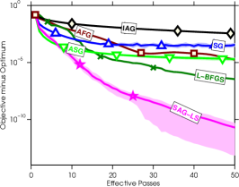
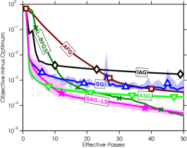
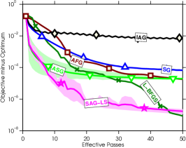
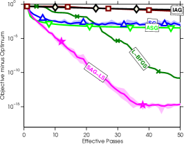

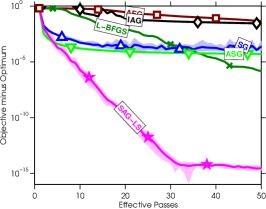
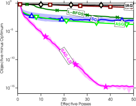
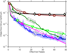
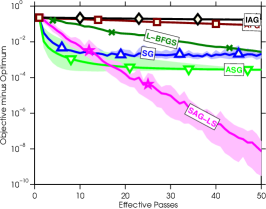
We plot the results of the different methods for the first effective passes through the data in Figure 1. For the stochastic methods, we plot the mean performance as well as the minimum and maximum function values across choices for the initial random seed. We can observe several trends across the experiments:
-
•
FG vs. SG: Although the performance of SG methods is known to be catastrophic if the step size is not chosen carefully, after giving the SG methods (SG and ASG) an unfair advantage (by allowing them to choose the best step-size in hindsight), the SG methods always do substantially better than the FG methods (AFG and L-BFGS) on the first few passes through the data. However, the SG methods typically make little progress after the first few passes. In contrast, the FG methods make steady progress and eventually the faster FG method (L-BFGS) typically passes the SG methods.
-
•
(FG and SG) vs. SAG: The SAG iterations seem to achieve the best of both worlds. They start out substantially better than FG methods, often obtaining similar performance to an SG method with the best step-size chosen in hindsight. But the SAG iterations continue to make steady progress even after the first few passes through the data. This leads to better performance than SG methods on later iterations, and on most data sets the sophisticated FG methods do not catch up to the SAG method even after passes through the data.
-
•
IAG vs. SAG: Even though these two algorithms differ in only the seemingly-minor detail of selecting data points at random (SAG) compared to cycling through the data (IAG), the performance improvement of SAG over its deterministic counterpart IAG is striking (even though the IAG method was allowed to choose the best step-size in hindsight). We believe this is due to the larger step sizes allowed by the SAG iterations, which would cause the IAG iterations to diverge.
5.2 Comparison to Coordinate Optimization Methods
For the -regularized logistic regression problem, an alternative means to take advantage of the structure of the problem and achieve a linear convergence rate with a cheaper iteration cost than FG methods is to use randomized coordinate optimization methods. In particular, we can achieve a linear convergence rate by applying coordinate descent to the primal [Nesterov, 2010] or coordinate-ascent to the dual [Shalev-Schwartz and Zhang, 2013b]. In our second experiment, we included the following additional methods in this comparison:
-
•
PCD: The randomized primal coordinate-descent method of Nesterov [2010], using a step-size of , where is the Lipschitz-constant with respect to coordinate of . Here, we sampled the coordinates uniformly.
-
•
PCD-L: The same as above, but sampling coordinates according to their Lipschitz constant, which can lead to an improved convergence rate [Nesterov, 2010].
-
•
DCA: Applying randomized coordinate ascent to the dual, with uniform example selection and an exact line-search [Shalev-Schwartz and Zhang, 2013b].
As with comparing FG and SG methods, it is difficult to compare coordinate-wise methods to FG and SG methods in an implementation-independent way. To do this in a way that we believe is fair (when discussing convergence rates), we measure the number of effective passes of the DCA method as the number of iterations of the method divided by (since each iteration accesses a single example as in SG and SAG iterations). We measure the number of effective passes for the PCD and PCD-L methods as the number of iterations multiplied by so that effective pass for this method has a cost of as in FG and SG methods. We ignore the additional cost associated with the Lipschitz sampling for the PCD-L method (as well as the expense incurred because the PCD-L method tended to favour updating the bias variable for sparse data sets) and we also ignore the cost of numerically computing the optimal step-size for the DCA method.
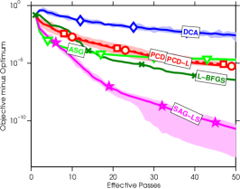
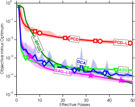
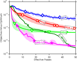
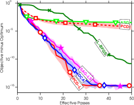
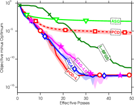
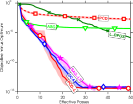
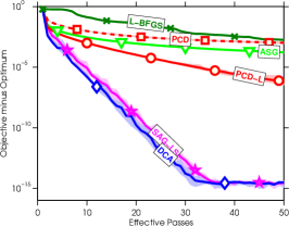
We compare the performance of the randomized coordinate optimization methods to several of the best methods from the previous experiment in Figure 2. In these experiments we observe the following trends:
-
•
PCD vs. PCD-L: For the problems with (top and bottom rows of Figure 2), there is little difference between uniform and Lipschitz sampling of the coordinates. For the problems with (middle row of Figure 2), sampling according to the Lipschitz constant leads to a large performance improvement over uniform sampling.
-
•
PCD vs. DCA: For the problems with , DCA and PCD-L have similar performance. For the problems with , the performance of the methods typically differed but neither strategy tended to dominate the other.
-
•
(PCD and DCA) vs. (SAG): For some problems, the PCD and DCA methods have performance that is similar to SAG-LS and the DCA method even gives better performance than SAG-LS on one data set. However, for many data sets either the PCD-L or the DCA method (or both) perform poorly while the SAG-LS iterations are among the best or substantially better than all other methods on every data set. This suggests that, while coordinate optimization methods are clearly extremely effective for some problems, the SAG method tends to be a more robust choice across problems.


5.3 Comparison of Step-Size Strategies
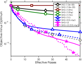
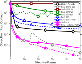
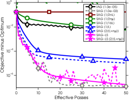
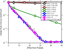
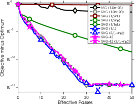
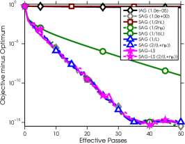
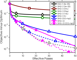
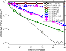
In our prior work we analyzed the step-sizes and [Le Roux et al., 2012], while Section 3 considers the choice and Section 4.5 discusses the choices and as in FG methods. In Figure 3 we compare the performance of these various strategies to the performance of the SAG algorithm with our proposed line-search as well as the IAG and SAG algorithms when the best step-size is chosen in hindsight. In this plot we see the following trends:
-
•
Proposition 1 of Le Roux et al. [2012]: Using a step-size of performs poorly, and makes little progress compared to the other methods. This makes sense because Proposition 1 in Le Roux et al. [2012] implies that the convergence rate (in terms of effective passes through the data) under this step size will be similar to the basic gradient method, which is known to perform poorly unless the problem is very well-conditioned.
-
•
Proposition 2 of Le Roux et al. [2012]: Using a step-size of performs extremely well on the data sets with (middle row). In contrast, for the data sets with it often performs very poorly, and in some cases appears to diverge. This is consistent with Proposition 2 in Le Roux et al. [2012], which shows a fast convergence rate under this step size only if certain conditions on hold.
-
•
Theorem 1: Using a step-size of performs consistently better than the smaller step size , but in some cases it performs worse than . However, in contrast to , the step size always has reasonable performance.
-
•
Section 4.5: The step size of performs performs extremely well on the data sets with , and performs better than the step sizes discussed above on all but one of the remaining data sets. The step size of seems to perform the same or slightly better than using except on one data set where it performs poorly.
-
•
Line-Search: Using the line-search from Section 4.6 tends to perform as well or better than the various constant step size strategies, and tends to have similar performance to choosing the best step size in hindsight.
-
•
IAG vs. SAG: When choosing the best step size in hindsight, the SAG iterations tend to choose a much larger step size than the IAG iterations. The step sizes chosen for SAG were to times larger than the step sizes chosen by IAG, and always lead to better performance by several orders of magnitude.

5.4 Effect of mini-batches
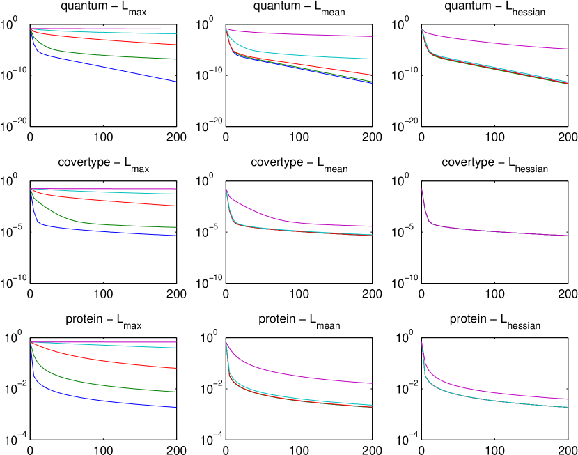
As we discuss in Section 4.7, when using mini-batches within the SAG iterations there is a trade-off between the higher iteration cost of using mini-batches and the faster convergence rate obtained using mini-batches due to the possibility of using a smaller value of . In Figure 4, we compare (on the dense data sets) the excess sub-optimality as a function of the number of examples seen for various mini-batch sizes and the three step-size strategies , , and discussed in Section 4.7.
Several conclusions may be drawn from these experiments:
-
•
Even though Theorem 1 hints at a maximum mini-batch size of without loss of convergence speed, this is a very conservative estimate. In our experiments, the original value of was on the order of and mini-batch sizes of up to 500 could be used without a loss in performance. Not only does this yield large memory storage gains, it would increase the computational efficiency of the algorithm when taking into account vectorization.
-
•
To achieve fast convergence, it is essential to use a larger step-size when larger mini-batches are used. For instance, in the case of the quantum dataset with a mini-batch size of , we have , and . In the case of the covertype dataset and for a mini-batch size of , we have , and .

5.5 Effect of non-uniform sampling
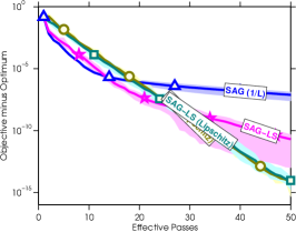
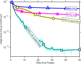
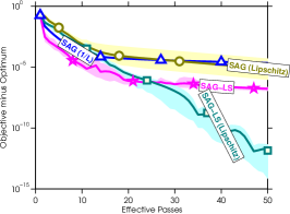
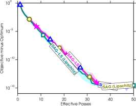
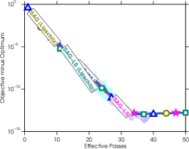
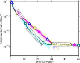
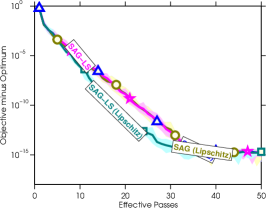
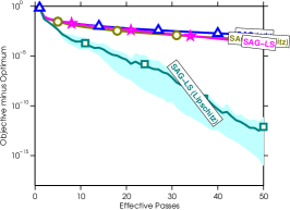
In our final experiment, we explored the effect of using the non-uniform sampling strategy discussed in Section 4.8. In Figure 5, we compare several of the SAG variants with uniform sampling to the following two methods based on non-uniform sampling:
-
•
SAG (Lipschitz): In this method we sample the functions in proporition to , where is the global Lipschitz constant of the corresponding and we set to the average of these constants, . Plugging in these values into the formula at the end of Section 4.8 and using to denote the maximum value, we set the step-size to .
-
•
SAG-LS (Lipschitz): In this method we formed estimates of the quantities , , and . The estimator is computed in the same way as the SAG-LS method. To estimate each , we keep track of an estimate for each and we set to the average of the values among the that we have sampled at least once. We set if example was not selected and otherwise we initialize to and perform the line-search until we have a valid (this means that will be approximately halved if we perform a full pass through the data set and never violate the inequality). To ensure that we do not ignore important unseen data points for too long, in this method we sample a previously unseen function with probability , and otherwise we sample from the previously seen in proportion to . To prevent relying too much on our initially-poor estimate of , we use a step size of , where is the step-size we normally use with uniform sampling and is the step-size we use with the non-uniform sampling method, so that the method interpolates between these extremes until the entire data set has been sampled.
We make the following observations from these experiments:
-
•
SAG (1/L) vs. SAG (Lipschitz): With access to global quantities and a constant step size, the difference between uniform and non-uniform sampling was typically quite small. However, in some cases the non-uniform sampling method behaved much better (top row of Figure 5).
-
•
SAG-LS vs. SAG-LS (Lipschitz): When estimating the Lipschitz constants of the individual functions, the non-uniform sampling strategy often gave better performance. Indeed, the adaptive non-uniform sampling strategy gave solutions that are orders of magnitude more accurate than any method we examined for several of the data sets (e.g., the protein, covertype, and sido data sets) In the context of logistic regression, it makes sense that an adaptive sampling scheme could lead to better performance, as many correctly-classified data samples might have a very slowly-changing gradient near the solution, and thus they do not need to be sampled often.

6 Discussion
Since the first version of this work was published [Le Roux et al., 2012], there has been an explosion of interest in stochastic methods with improved convergence rates. In this section we first review other algorithms that have been discovered to have this property, and then we discuss the many possible variants on these basic algorithms that have been explored. As this is a very quickly-evolving area there are likely to be many new developments in the near future, but we note that this literature review is up to date as of January, 2015.
6.1 Alternative Algorithms
SDCA: The first algorithm that was shown to have a similar convergence rate and iteration cost to SAG was in fact a much older algorithm: coordinate optimization applied to a dual problem with randomized coordinate selection, referred to as stochastic dual coordinate ascent (SDCA). Shalev-Schwartz and Zhang [2013b] consider the problem of minimizing an -regularized finite sum,
where each is convex and each is Lipschitz-continuous, by optimizing its Fenchel dual,
They consider applying exact coordinate optimization to a randomly selected coordinate. Using the primal-dual relationship , they show a linear convergence rate in terms of the duality gap. Since there is one dual variable associated with each example , the iteration cost is independent of and thus the strategy has similar convergence properties to SAG (the memory requirements are identical in this context, see Section 4.1).
This result is related to the earlier result of [Nesterov, 2010], who shows a similar convergence rate for randomized coordinate descent.777Local linear convergence rates of deterministic coordinate descent methods had been established much earlier [Luo and Tseng, 1992]. However, the result of Nesterov cannot be directly applied to the dual problem in general since the dual does not necessarily have a Lipschitz-continuous gradient. A similar result was also reported even earlier by Collins et al. [2008] without requiring that the gradient of the dual is Lipschitz-continuous, but this result again only applied to the dual objective. More recently, Shalev-Schwartz and Zhang [2013a] show linear convergence of SDCA in the more general setting
where are matrices and is strongly convex. They also relax the requirement of exact coordinate optimization, providing a variety of more practical alternatives. Further, in subsequent work they obtain a convergence rate in the convex case by adding an explicit strongly-convex regularizer to the problem [Shalev-Schwartz and Zhang, 2014].
A disadvantage of SDCA compared to the SAG algorithm is that the SDCA convergence rates depend on rather than the strong-convexity constant . In the worst case we have , but if is much larger then the convergence rate of SAG is much faster. Further, even in cases where , the convergence rate of SAG might be much faster if the iterates stay in local region with a higher strong-convexity constant. As an extreme example, due to local strong-convexity SAG might have a linear convergence rate in scenarios where SDCA has a sub-linear convergence. This subtle but practically important issue was a key focus in the recent work of [Agarwal and Bottou, 2014], and indeed the performance of SDCA was very poor on three of the test problems in our experiments. See Figure 2 (top left, top right, bottom right).
MISO: Mairal [2013] analyzes a very general surrogate optimization framework, that includes a wide vareity of existing algorithms. He also considers incremental algorithms in this framework, and specialized to the smooth and unconstraeind setting (with a ‘Lipschitz surrogate’) obtains an algorithm (MISO) that is very similar to the SAG algorithm,
where is defined as in the SAG algorithm 6, and is the parameter vector used to compute the corresponding . Thus, instead of applying the SAG step to , MISO applies the step to the average of the previous values used to form the current variables. Mairal [2013] shows that this algorithm also achieves an rate for convex objectives and a linear convergence rate for strongly-convex objectives.
However, MISO has the disadvantage that it not only requires storing the gradient values but also storing previous iterations (which are less likely to have a nice structure). Further, the linear convergence rate shown for MISO is substantially slower than the convergence rate shown in Theorem 1. In particular, the rate is more similar to the substantially slower Proposition 1 in our prior work [Le Roux et al., 2012]. Subsequent work on the MISO algorithm has shown an analogous result to Proposition 2 in our prior work; if the is sufficiently larger than , then using a step-size proportional to yields a faster convergence rate [Mairal, 2014, Defazio et al., 2014b]. However, using this step-size causes divergence if is not sufficiently large.
SVRG: Another interesting framework that has been considered is known as ‘mixed optimization’, ‘stochastic variance-reduced gradient’ (SVRG), or ‘semi-stochastic gradient descent’ (S2GD) [Mahdavi and Jin, 2013, Johnson and Zhang, 2013, Zhang et al., 2013, Konečnỳ and Richtárik, 2013].888Wang et al. [2013] consider a related algorithm that maintains an easily-computable approximation to the current gradient . Although this can improve the constants in the sublinear SG convergence rates, it does not improve the rates. Unlike FG methods that utilize the full gradient and SG methods that consider individual gradients , these mixed optimization methods combine the two. In particular, they use a (possibly regularized) iteration of the form
where is the last iterate where the full gradient was evaluated. The algorithm alternates between computing the full gradient at , and performing some number of stochastic gradient iterations. Note this is very similar to the SAG algorithm written in the form
where is defined as in the MISO algorithm. These methods are thus similar to SAG in the use of potentially-outdated gradient information, but differ in that the outdated gradients are all computed at the same previous iteration and the weighting of terms is changed. If the step-size and parameter are set appropriately, this algorithm has a linear convergence rate in the strongly-convex case. It can also achieve an convergence rate in the general convex case, by applying it to a purturbed problem where a strongly-convex regularizer has been added.
A key advantage of this strategy is it only requires storing , rather than the gradient values. However, to obtain this improved memory requirement we must evaluate twice on each iteration. Further, the algorithm innefficiently requires full passes through the data to evaluate for all .
A disadvantage of the SVRG method is that it requires setting two parameters (rather than one) and the convergence rate depends in a non-trivial way on their interaction both with each other and with both the Lipschitz constant and the strong-convexity. As with SDCA, the dependence on the strong-convexity constant is notable. In particular, the algorithm can’t be applied without modification to general convex problems, and (although the effect is not as severe as it is with SDCA) the convergence rate may be substantially slower than SAG if there exists hidden strong convexity.
Self-Concordant Objectives: A surprising recent development is that Bach and Moulines [2013] have shown that the finite sum assumption is not required to obtain the convergence rate in the special case of least squares. They show that an averaged SG method achieves this rate, and give a 2-phase Newton-like SG method that achieves this rate under an assumption similar to self-concordance. However, this assumption does not hold in general for the class of problems considered here.
SAGA: One of the most recent developments in this area is the SAGA algorithm Defazio et al. [2014a]. This algorithm intelligently combines the updates used in the SAG and SVRG algorithms. This method maintains the appealing properties of SAG, but yields a simpler proof. However, the proof technique used in that work does not yield a simpler analysis of the original SAG algorithm.
Lower Bounds: There has been recent work on determining a lower bound on the convergence rate that can be expected for minimizing finite sums. Defazio et al. [2014b] show that the rate must be at least in the strongly-convex case, while Agarwal and Bottou [2014] establish a bound that also depends on the condition number .
6.2 Generalizations and Other Issues
Accelerated gradient: AFG methods are variants of the basic FG method that can obtain an convergence rate for the general convex case, and faster linear convergence rates that depend on the square root of the condition number rather than the condition number in the strongly-convex case [see Nesterov, 2004, §2.2.1]. For strongly-convex objectives, it has been shown that a mini-batch strategy can obtain a better dependence on the condition number in certain regimes for SDCA [Shalev-Shwartz and Zhang, 2013] and more recently for SVRG [Nitanda, 2014]. It is possible that similar arguments could hold for SAG algorithms, which could be advantageous over these methods for reasons discussed in the previous section.
Shalev-Schwartz and Zhang [2014] have also given an accelerated version of the SDCA method for ill-conditioned problems, that uses SDCA to solve a sequence of regularized problems up to a prescribed optimality. Since this procedure ultimately relies on the sequence of primal solutions, we can also accelerate SAG using a procedure like this. However, a difficulty with this procedure (whether SAG or SDCA are used) is the cost of measuring the optimality of the sub-problems.
Rather than using this inner-outer procedure, Lin et al. [2014] show that using a deterministic primal iteration (based on the full data set) allows one to construct a primal solution that has the accelerated rate from the result of an accelerated dual coordinate ascent method. Zhang and Xiao [2014] give a coordinate-wise variant of the accelerated primal-dual method of Chambolle and Pock [2011] that also achieves this rate. Based on these results, it is possible that accelerated versions of SAG could be developed that do not rely on an inner-outer procedure.
The convergence rates of these accelerated methods have the same form as the lower bound established by Agarwal and Bottou [2014]. However, Agarwal and Bottou point out that these accelerated convergence rates depend on rather than . Thus, they conclude that the basic SAG algorithm may still be much faster on some problems than accelerated SDCA methods, and indeed show how to construct a problem where SAG is arbitrarily faster than accelerated SDCA. The possibility of developing an accelerated SAG algorithm that is adaptive to remains open.
Proximal gradient and ADMM: It is becoming increasingly common to address problems of the form
where and satisfy our assumptions and is a general convex function that could be non-smooth or enforce that constraints are satisfied. Proximal-gradient methods for problems with this structure use iterations of the form
where the prox operator is the solution to the proximity problem
Proximal-gradient and accelerated proximal-gradient methods are appealing for solving non-smooth optimization problems because they achieve the same convergence rates as FG methods for smooth optimization problems [Nesterov, 2007, Schmidt et al., 2011]. We have explored a variant of the proximal-gradient method where the average over the values is replaced by the SAG approximation (6). Although our analysis does not directly apply to this scenario, we believe that this proximal-SAG algorithm for composite non-smooth optimization achieves the same convergence rates as the SAG algorithm for smooth optimization; this is supported by the experiments of Xiao and Zhang [2014]. Indeed, there now exist proximal-gradient variants of SDCA [Shalev-Schwartz and Zhang, 2013a], MISO [Mairal, 2013], SVRG [Xiao and Zhang, 2014], and SAGA [Defazio et al., 2014a].
In cases where is composed with a linear function, we can consider approaches based on the alternating direction method of multipliers (ADMM). This has been explored for SDCA [Suzuki, 2014] and MISO [Zhong and Kwok, 2014], and a variant based on SAG is also likely to be possible.
Coordinate-wise: The key advantage of SG and SAG methods is that the iteration cost is independent of the number of functions . However, in many applications we may also be concerned with the dependence of the iteration cost on the number of variables . Randomized coordinate-wise methods offer linear convergence rates with an iteration cost that is linear in but independent of [Nesterov, 2010]. We can consider a variant of SAG whose iteration cost is independent of both and by using the update
to each coordinate of each vector in the SAG algorithm, and where is a sample from the set . Konečnỳ et al. [2014] recently proposed an SVRG algorithm of this flavour.
Newton-like: In cases where is twice-differentiable, we can also consider Newton-like variants of the SAG algorithm,
where is a positive-definite approximation to the inverse Hessian . We would expect to obtain a faster convergence rate by using an appropriate choice of the sequence . However, in order to not increase the iteration cost these matrices should be designed to allow fast multiplication. For example, we could choose to be diagonal, which would also preserve any sparsity present in the updates. Sohl-Dickstein et al. [2014] propose a quasi-Newton method in this class that shows impressive empirical results, although the iteration cost is much higher.
Relaxing Convexity Assumptions: It is likely that the convexity assumptions made in this work could be relaxed. For example, Gong and Ye [2014] show SVRG can obtain a linear convergence under weaker assumptions. Since SAG is adaptive to hidden strong-convexity, the assumptions needed for its linear convergence are likely even weaker. Further, the SAG algorithm may also be useful even if is non-convex (which is different than SDCA). In this case we expect that, similar to the IAG method [Blatt et al., 2007], the algorithm converges to a stationary point under very general conditions.
Non-Uniform Sampling: We have given an argument that non-uniform sampling should benefit the SAG algorithm, and shown empirically that it can lead to a substantial improvement. However, we have not yet given a full analysis of this scheme. Subsequent works have shown that the type of dependency we conjecture here (e.g., dependence on the average Lispschitz constant) can be achieved with non-uniform sampling in the context of SDCA [Qu et al., 2014, Zhao and Zhang, 2014], SVRG [Xiao and Zhang, 2014], and SAGA [Schmidt et al., 2015]
Step-size selection and termination criteria: The three major disadvantages of SG methods are: (i) the slow convergence rate, (ii) deciding when to terminate the algorithms, and (iii) choosing the step size while running the algorithm. This work shows that the SAG iterations achieve a much faster convergence rate, but the SAG iterations may also be advantageous in terms of termination criteria and choosing step sizes. In particular, the SAG iterations suggest a natural termination criterion; since the quantity in Algorithm 1 converges to as converges to zero, we can use as an approximation of the optimality of as the iterates converge. Regarding choosing the step-size, a disadvantage of a constant step-size strategy is that a step-size that is too large may cause divergence. But, we expect that it is possible to design line-search or trust-region strategies that avoid this issue. Such strategies might even lead to faster convergence for functions that are locally well-behaved around their optimum, as indicated in our experiments. Further, while SG methods require specifying a sequence of step sizes and mis-specifying this sequence can have a disastrous effect on the convergence rate [see Nemirovski et al., 2009, §2.1], our theory shows that the SAG iterations achieve a fast convergence rate for any sufficiently small constant step size, and our experiments indicate that a simple line-search gives strong performance.
Acknowledgements
We would like to thank the anonymous reviewers for their many useful comments. This work was partially supported by the European Research Council (SIERRA-ERC-239993) and a Google Research Award. Mark Schmidt is also supported by a postdoctoral fellowship from the Natural Sciences and Engineering Research Council of Canada.
Appendix A: Comparison of convergence rates
We now present a comparison of the convergence rates of primal and dual FG and coordinate-wise methods to the rate of the SAG method in terms of effective passes through the data for -regularized least-squares regression. In particular, in this appendix we will consider the problem
where to apply the SG or SAG method we can use
If we use to denote a vector containing the values and to denote a matrix withs rows , we can re-write this problem as
The Fenchel dual of this problem is
We can obtain the primal variables from the dual variables by the formula . Convergence rates of different primal and dual algorithms are often expressed in terms of the following Lipschitz constants:
| (Lipschitz constant of ) | |||
| (Lipschitz constant for all ) | |||
| (Lipschitz constant of all ) | |||
| (Lipschitz constant of ) | |||
| (Lipschitz constant of all ) |
Here, we use to denote the maximum eigenvalue of , to denote the maximum squared row-norm , and to denote the maximum squared column-norm . We use to refer to element of of , and similarly for . The convergence rates will also depend on the primal and dual strong-convexity constants:
| (Strong-convexity constant of ) | |||
| (Strong-convexity constant of ) |
Here, is the minimum eigenvalue of , and is the minimum eigenvalue of .
A.3 Full Gradient Methods
Using a similar argument to [Nesterov, 2004, Theorem 2.1.15], if we use the basic FG method with a step size of , then converges to zero with rate
while a larger step-size of gives a faster rate of
and we see that the speed improvement is determined by how much smaller is than .
If we use the basic FG method on the dual problem with a step size of , then converges to zero with rate
and with a step-size of the rate is
Thus, whether we can solve the primal or dual method faster depends on and . In the over-determined case where has independent columns, a primal method should be preferred. In the under-determined case where has independent rows, we can solve the dual more efficiently. However, we note that a convergence rate on the dual objective does not necessarily yield the same rate in the primal objective. If is invertible (so that ) or it has neither independent columns nor independent rows (so that ), then there is no difference between the primal and dual rates.
The AFG method achieves a faster rate. Applied to the primal with a step-size of it has a rate of [Nesterov, 2004, Theorem 2.2.2]
and applied to the dual with a step-size of it has a rate of
A.4 Coordinate-Descent Methods
The cost of applying one iteration of an FG method is . For this same cost we could apply iterations of a coordinate descent method to the primal, assuming that selecting the coordinate to update has a cost of . If we select coordinates uniformly at random, then the convergence rate for iterations of coordinate descent with a step-size of is [Nesterov, 2010, Theorem 2]
Here, we see that applying a coordinate-descent method can be much more efficient than an FG method if . This can happen, for example, when the number of variables is much larger than the number of examples . Further, it is possible for coordinate descent to be faster than the AFG method if the difference between and is sufficiently large.
For the cost of one iteration of the FG method, we could alternately perform iterations of coordinate descent on the dual problem. With a step size of this would obtain a rate on the dual objective of
which will be faster than the dual FG method if . This can happen, for example, when the number of examples is much larger than the number of variables . The difference between the primal and dual coordinate methods depends on compared to and compared to .
The analysis of SDCA gives a convergence rate in terms of the duality gap (and hence the primal) rather than simply in terms of the dual Shalev-Schwartz and Zhang [2013b]. Using the SDCA analysis, we obtain a rate in the duality gap of
which is the same as the dual rate given above when , and is slower otherwise.
A.5 Stochastic Average Gradient
For the cost of one iteration of the FG method, we can perform iterations of SAG. With a step size of , performing iterations of the SAG algorithm has a rate of
In the case where , this is most similar to the rate obtained with the dual coordinate descent method, though there is a constant factor of and the rate depends on the primal strong convexity constant rather than the dual . However, in this case the SAG rate will often be faster because the term in the denominator is replaced by . An interesting aspect of the SAG rate is that unlike other methods the convergence rate of SAG reaches a limit: the convergence rate improves as grows and as the condition number decreases but no further improvement in the convergence rate is obtained beyond the point where . Thus, while SAG may not be the method of choice for very well-conditioned problems, it is a robust choice as it will always tend to be among the best methods in most situations.
Appendix B: Proof of the theorem
In this Appendix, we give the proof of Theorem 1.
B.3 Problem set-up and notation
Recall that we use to denote a -strongly convex function, where the functions for are convex functions from to with -Lipschitz continuous gradients. In this appendix we will use the convention that so that the regular convex case (where ) is allowed. We assume that a minimizer of is attained by some parameter (such a value always exists and is unique when ).
Recall that the SAG algorithm performs the recursion (for ):
where an integer is selected uniformly at random from and we set
We will use the notation
and we will also find it convenient to use
| (17) |
With this notation, note that and .
For a square matrix , we use to denote a vector of size composed of the diagonal of , while for a vector of dimension , is the diagonal matrix with on its diagonal. Thus is a diagonal matrix with the diagonal elements of on its diagonal, and .
In addition, if is a matrix and is a matrix, then we will use the convention that:
-
•
is the matrix being the concatenation of the ()-blocks on the diagonal of ;
-
•
is the block-diagonal matrix whose ()-blocks on the diagonal are equal to the ()-blocks of .
Finally, will denote the -field of information up to (and including) time . In other words, is the -field generated by . Given , we can write the expected values of the and variables in the SAG algorithm as
The proof is based on finding a Lyapunov function from to such that the sequence decreases at an appropriate rate, and dominates . We derive these results in a parameterized way, leaving a variety of coefficients undetermined but tracking the constraints required of the coefficients as we go. Subsequently, we guide the setting of these coefficients by using a second-order cone solver, and verify the validity of the resulting coefficients using a symbolic solver to check positivity of certain polynomials. Finally, the constants in the convergence rate are given by the initial values of the Lyapunov function, based on the choice of .
The Lyapunov function contains a term of the form for some values of , and . Our analysis makes use of the following lemma, derived in [Le Roux et al., 2012, Appendix A.4], showing how this quadratic form evolves through the SAG recursion in terms of the elements of .
Lemma 1.
If , for , and , then
with
Our proof also uses the following lemma, giving the inverse of a highly-structured matrix that arises in the analysis.
Lemma 2.
Let be the identity in and be defined by stacking identity matrices in as in (17). If and are non-zero real-valued scalars, then it holds that
Proof.
It is sufficient to verify that the inverse of the left side times the right side is equal to the identity matrix,
where we use that , giving . ∎
B.4 General Lyapunov function
For some , we consider a Lyapunov function of the form
with
To achieve the desired convergence rate, our goal is to show for appropriate values of and that
almost surely. Thus, in addition to the algorithm parameter , there are 2 parameters of the result {, } and 6 parameters of the Lyapunov function {, , , , , }.
B.5 Lyapunov upper bound
To show (a), we derive an upper bound on the quantity
Lemma 1 gives an expression for the expectation over the quadratic term in the last line, and we will have
We also use that strong convexity of implies
| (18) |
Further, using the Lipschitz-continuity of and the identity , followed by applying Lemma 1 using to expand the last term, gives us the bound
| (19) | ||||
Combining Lemma 1 with Inequalities (18) and (19) yields an upper bound on with a large number of terms. To help in the process of simplifying these terms, Table 3 lists all the terms up to a scalar factor and possibly a matrix . The table also gives these scalars and matrices for each term, as well as the source of the term.
| Term | Scalar | Matrix | Source | Group |
| 0 | ||||
| 0 | ||||
| 3 and 4 | ||||
| 5 | ||||
| 9 | ||||
| Inequality (18) | 0 | |||
| Inequality (18) | 7 | |||
| Inequality (18) | 4 | |||
| Inequality (19) | 0 | |||
| Inequality (19) | 7 | |||
| Inequality (19) | 2 | |||
| Inequality (19) | 3 and 4 | |||
| Inequality (19) | 8 | |||
| Inequality (19) | 6 and 7 | |||
| Lemma 1 | 3 and 4 | |||
| Lemma 1 | 5 | |||
| Lemma 1 | 9 | |||
| Lemma 1 | 8 | |||
| Lemma 1 | 6 and 7 | |||
| Lemma 1 | 1 |
We combine the expressions from Table 3 using the stated groups in the last column. For example, we add together all the terms in group to obtain a scalar coefficient for terms in this group. We do this in the straightforward way (using that and ) for groups , , , , , and . For groups and we split into terms that have an identity matrix () and terms with an term (). Similarly, comes from terms with an identity matrix in and correspond to terms with an term. Combining expressions in this way (and adding/subtracting ) gives:
with
In this expression, only appears through a quadratic form, with a quadratic term . If and , then this quadratic term is non-positive and we may maximize in closed form with respect to to obtain an upper bound. Assuming that and , we use Lemma 2, , to obtain:
By using Lipschitz continuity of each to observe that , we obtain:
with
In order to show the decrease of the Lyapunov function, we need to show that for all .
If we assume that and , then we have by strong-convexity
and thus the condition is that
And if we want to show that , then it suffices to have and .
B.6 Domination of
By again using the strong convexity of (as in (18)), we have
using the smoothness of and the assumption that .
Thus, in order for to dominate we require the additional constraints
B.7 Finding constants
Given the algorithm and result parameters , we have the following constraints:
| (Constraint 1) | ||||
| (Constraint 2) | ||||
| (Constraint 3) | ||||
| (Constraint 4) | ||||
| (Constraint 5) | ||||
| (Constraint 6) | ||||
| (Constraint 7) | ||||
| (Constraint 8) | ||||
| (Constraint 9) |
We also require , but this will follow from Constraint 8 since we will have . All of the constraints above are convex in , , , , , . Thus, given candidate values for the remaining values, the feasibility of these constraints may be checked using a numerical toolbox (as a second-order cone program). However, these parameters should be functions of and should be valid for all . Thus, given a sampling of values of and , representing these parameters as polynomials in , the candidate functions may be found through a second-order cone programs.
By experimenting with this strategy, we have come up with the following values for the constants:
We will assume , since the result for follows because SAG is equivalent to gradient descent in this case. Under this assumption, we see that Constraints 1 and 2 are satisfied by the above parameterizaiton. Below we verify that Constraints 3-9 are also satisfied using symbolic computations in Matlab (the code used in this section is available on the first author’s webpage). Specifically, we parameterize the constraints as polynomials and then verify that the polynomials are positive over an appropriate interval using the function below (which simply checks that no roots of the polynomial lie in the interval , and that is positive at the mid-point of the interval).
![[Uncaptioned image]](/html/1309.2388/assets/isPositive.png)
B.8 Verifying the result
To verify the result under these constants, we consider whether or . In , we discard the term of the form , which does not impact the validity of our result. Moreover, without loss of generality, we may assume and .
B.8.1 Well-conditioned problems ()
In this situation, it suffices to show the result for since, (a) if a function is -strongly convex, then it is -strongly convex for all smaller , and (b) the final inequality does not involve . All constraints (when properly multiplied where appropriate by ) can be written as rational functions of :
| (Constraint 3) | |||
| (Constraint 4) | |||
| (Constraint 5) | |||
| (Constraint 6) | |||
| (Constraint 7) | |||
| (Constraint 8) | |||
| (Constraint 9) |
We only need to check the positivity of these polynomials in . We do this using the function above, via the script below. Note that we also have and for .
![[Uncaptioned image]](/html/1309.2388/assets/largeMu.png)
B.8.2 Ill-conditioned problems ()
We consider the variables and , so that . We may express all quantities using and . The difficulty here is that we have two variables. We first check the dependency in terms of of the expressions , , and . These are univariate polynomials with an affine dependence on , so their positivity can be checked by checking positivity for or . Again making use of symbolic computation, we can deduce that
| (Constraint 3) | |||
| (Constraint 4) | |||
We include below the additional commands to verify these properties:
![[Uncaptioned image]](/html/1309.2388/assets/smallMu1.png)
Given the monotonicity of the bounds in and , we only need to check our results for the smaller values of and , i.e., for . Similarly, because of the monotonicity in the term , we may replace by times its upper-bound (i.e., its value at ). Also note that is divisble by , and we have and for . Using this, we can show that Constraints 5-9 are satisfied by checking the positivity of the following polynomials:
| (Constraint 5) | |||
| (Constraint 6) | |||
| (Constraint 7) | |||
| (Constraint 8) | |||
| (Constraint 9) |
Constraints 5-7 are affine in and we thus only need to check positivity for and .
![[Uncaptioned image]](/html/1309.2388/assets/smallMu2a.png)
The other two expressions (Constraints 8 and 9) are more complicated as there are second-order polynomials in . If , they have positive second derivatives, negative derivatives at and , and positive values at . They are thus positive, which is verified by the code below.
![[Uncaptioned image]](/html/1309.2388/assets/smallMu2b.png)
For the remaining scenarios where , we have a fixed so we can check the positivity of the polynomials in . A Matlab script that does the steps above in addition to checking these not-particularly-interesting cases is available from the first author’s web page.
B.9 Convergence Rate
We have that
and that
In the strongly-convex case (), combining these gives us the linear convergence rate
In the convex case ( and ), we have by convexity that
We then have
Summing this up to iteration yields
Finally, by Jensen’s inequality note that
so with we have
B.10 Intial values of Lyapunov function
To obtain the results of Theorem 1, all that remains is computing the initial value of the Lyapunov function for the two initializations.
B.10.1 Initialization with the zero vector
If we initialize with we have
Plugging in the values of our parameters,
and using we obtain (noting that )
B.10.2 Initialization with average gradient
If we initialize with we have, by noting that we still have ,
By observing that and using [Nesterov, 2004, Equations 2.17], we can bound the norm in the second term as follows:
Using this in the Lyapunov function we obtain
References
- Agarwal and Bottou [2014] A. Agarwal and L. Bottou. A lower bound for the optimization of finite sums. arXiv preprint, 2014.
- Agarwal et al. [2012] A. Agarwal, P. L. Bartlett, P. Ravikumar, and M. J. Wainwright. Information-theoretic lower bounds on the oracle complexity of stochastic convex optimization. IEEE Transactions on Information Theory, 58(5), 2012.
- Bach and Moulines [2011] F. Bach and E. Moulines. Non-asymptotic analysis of stochastic approximation algorithms for machine learning. Advances in Neural Information Processing Systems, 2011.
- Bach and Moulines [2013] F. Bach and E. Moulines. Non-strongly-convex smooth stochastic approximation with convergence rate . arXiv preprint, 2013.
- Bertsekas [1997] D. P. Bertsekas. A new class of incremental gradient methods for least squares problems. SIAM Journal on Optimization, 7(4):913–926, 1997.
- Blatt et al. [2007] D. Blatt, A. O. Hero, and H. Gauchman. A convergent incremental gradient method with a constant step size. SIAM Journal on Optimization, 18(1):29–51, 2007.
- Bordes et al. [2009] Antoine Bordes, Léon Bottou, and Patrick Gallinari. Sgd-qn: Careful quasi-newton stochastic gradient descent. Journal of Machine Learning Research, 10:1737–1754, 2009.
- Bottou and LeCun [2003] L. Bottou and Y. LeCun. Large scale online learning. Advances in Neural Information Processing Systems, 2003.
- Carbonetto [2009] P. Carbonetto. New probabilistic inference algorithms that harness the strengths of variational and Monte Carlo methods. PhD thesis, Univ. of British Columbia, May 2009.
- Caruana et al. [2004] R. Caruana, T. Joachims, and L. Backstrom. KDD-cup 2004: results and analysis. ACM SIGKDD Newsletter, 6(2):95–108, 2004.
- Cauchy [1847] A.L. Cauchy. Méthode générale pour la résolution des systèmes d’équations simultanées. Comptes rendus des séances de l’Académie des sciences de Paris, 25:536–538, 1847.
- Chambolle and Pock [2011] Antonin Chambolle and Thomas Pock. A first-order primal-dual algorithm for convex problems with applications to imaging. Journal of Mathematical Imaging and Vision, 40(1):120–145, 2011.
- Collins et al. [2008] M. Collins, A. Globerson, T. Koo, X. Carreras, and P.L. Bartlett. Exponentiated gradient algorithms for conditional random fields and max-margin markov networks. The Journal of Machine Learning Research, 9:1775–1822, 2008.
- Cormack and Lynam [2005] G. V. Cormack and T. R. Lynam. Spam corpus creation for TREC. In Proc. 2nd Conference on Email and Anti-Spam, 2005. http://plg.uwaterloo.ca/~gvcormac/treccorpus/.
- Defazio et al. [2014a] Aaron Defazio, Francis Bach, and Simon Lacoste-Julien. Saga: A fast incremental gradient method with support for non-strongly convex composite objectives. Advances in Neural Information Processing Systems, 2014a.
- Defazio et al. [2014b] Aaron J Defazio, ANUEDU AU, Tibério S Caetano, NICTA COM AU, and Justin Domke. Finito: A faster, permutable incremental gradient method for big data problems. International Conference on Machine Learning, 2014b.
- Delyon and Juditsky [1993] B. Delyon and A. Juditsky. Accelerated stochastic approximation. SIAM Journal on Optimization, 3(4):868–881, 1993.
- Duchi et al. [2011] John Duchi, Elad Hazan, and Yoram Singer. Adaptive subgradient methods for online learning and stochastic optimization. Journal of Machine Learning Research, 12:2121–2159, 2011.
- Frank and Asuncion [2010] A. Frank and A. Asuncion. UCI machine learning repository, 2010. URL http://archive.ics.uci.edu/ml.
- Friedlander and Schmidt [2012] M. P. Friedlander and M. Schmidt. Hybrid deterministic-stochastic methods for data fitting. SIAM Journal of Scientific Computing, 34(3):A1351–A1379, 2012.
- Ghadimi and Lan [2010] S. Ghadimi and G. Lan. Optimal stochastic approximation algorithms for strongly convex stochastic composite optimization. Optimization Online, July, 2010.
- Gong and Ye [2014] Pinghua Gong and Jieping Ye. Linear convergence of variance-reduced projected stochastic gradient without strong convexity. arXiv preprint, 2014.
- Guyon [2008] I. Guyon. Sido: A phamacology dataset, 2008. URL http://www.causality.inf.ethz.ch/data/SIDO.html.
- Hazan and Kale [2011] E. Hazan and S. Kale. Beyond the regret minimization barrier: an optimal algorithm for stochastic strongly-convex optimization. Conference on Learning Theory, 2011.
- Hu et al. [2009] C. Hu, J.T. Kwok, and W. Pan. Accelerated gradient methods for stochastic optimization and online learning. Advances in Neural Information Processing Systems, 2009.
- Johnson and Zhang [2013] R. Johnson and T Zhang. Accelerating stochastic gradient descent using predictive variance reduction. Advances in Neural Information Processing Systems, 2013.
- Keerthi and DeCoste [2005] S.S. Keerthi and D. DeCoste. A modified finite newton method for fast solution of large scale linear svms. Journal of Machine Learning Research, 6:341–361, 2005.
- Kesten [1958] H. Kesten. Accelerated stochastic approximation. Annals of Mathematical Statistics, 29(1):41–59, 1958.
- Konečnỳ and Richtárik [2013] Jakub Konečnỳ and Peter Richtárik. Semi-stochastic gradient descent methods. arXiv preprint, 2013.
- Konečnỳ et al. [2014] Jakub Konečnỳ, Zheng Qu, and Peter Richtárik. Semi-stochastic coordinate descent. arXiv preprint, 2014.
- Kushner and Yin [2003] H. J. Kushner and G. Yin. Stochastic approximation and recursive algorithms and applications. Springer-Verlag, Second edition, 2003.
- Lacoste-Julien et al. [2013] S. Lacoste-Julien, M. Jaggi, M. Schmidt, and P. Pletscher. Block-coordinate frank-wolfe optimization for structural svms. International Conference on Machine Learning, 2013.
- Le Roux et al. [2012] N. Le Roux, M. Schmidt, and F. Bach. A stochastic gradient method with an exponential convergence rate for strongly-convex optimization with finite training sets. Advances in Neural Information Processing Systems, 2012.
- Lewis et al. [2004] D.D. Lewis, Y. Yang, T. Rose, and F. Li. RCV1: A new benchmark collection for text categorization research. Journal of Machine Learning Research, 5:361–397, 2004.
- Lin et al. [2014] Qihang Lin, Zhaosong Lu, and Lin Xiao. An accelerated proximal coordinate gradient method and its application to regularized empirical risk minimization. arXiv preprint, 2014.
- Liu et al. [2009] J. Liu, J. Chen, and J. Ye. Large-scale sparse logistic regression. ACM SIGKDD Conference on Knowledge Discovery and Data Mining, 2009.
- Luo and Tseng [1992] Zhi-Quan Luo and Paul Tseng. On the convergence of the coordinate descent method for convex differentiable minimization. Journal of Optimization Theory and Applications, 72(1):7–35, 1992.
- Mahdavi and Jin [2013] M. Mahdavi and R. Jin. Mixedgrad: An ) convergence rate algorithm for stochastic smooth optimization. Advances in Neural Information Processing Systems, 2013.
- Mairal [2013] Julien Mairal. Optimization with first-order surrogate functions. International Conference on Machine Learning, 2013.
- Mairal [2014] Julien Mairal. Incremental majorization-minimization optimization with application to large-scale machine learning. arXiv preprint, 2014.
- Martens [2010] J. Martens. Deep learning via Hessian-free optimization. International Conference on Machine Learning, 2010.
- Nedic and Bertsekas [2000] A. Nedic and D. Bertsekas. Convergence rate of incremental subgradient algorithms. In Stochastic Optimization: Algorithms and Applications, pages 263–304. Kluwer Academic, 2000.
- Needell et al. [2014] D. Needell, N. Srebro, and R. Ward. Stochastic gradient descent, weighted sampling, and the randomized Kaczmarz algorithm. Advances in Neural Information Processing Systems, 2014.
- Nemirovski and Yudin [1983] A. Nemirovski and D. B. Yudin. Problem complexity and method efficiency in optimization. Wiley, 1983.
- Nemirovski et al. [2009] A. Nemirovski, A. Juditsky, G. Lan, and A. Shapiro. Robust stochastic approximation approach to stochastic programming. SIAM Journal on Optimization, 19(4):1574–1609, 2009.
- Nesterov [1983] Y. Nesterov. A method for unconstrained convex minimization problem with the rate of convergence . Doklady AN SSSR, 269(3):543–547, 1983.
- Nesterov [2004] Y. Nesterov. Introductory lectures on convex optimization: A basic course. Springer, 2004.
- Nesterov [2007] Y. Nesterov. Gradient methods for minimizing composite objective function. CORE Discussion Papers, 2007.
- Nesterov [2009] Y. Nesterov. Primal-dual subgradient methods for convex problems. Mathematical programming, 120(1):221–259, 2009.
- Nesterov [2010] Y. Nesterov. Efficiency of coordinate descent methods on huge-scale optimization problems. CORE Discussion Paper, 2010.
- Nesterov [2005] Yu Nesterov. Smooth minimization of non-smooth functions. Mathematical Programming, 103(1):127–152, 2005.
- Nitanda [2014] Atsushi Nitanda. Stochastic proximal gradient descent with acceleration techniques. Advances in Neural Information Processing Systems, 2014.
- Nocedal and Wright [2006] J. Nocedal and S. J. Wright. Numerical Optimization. Springer, New York, second edition, 2006.
- Polyak and Juditsky [1992] B. T. Polyak and A. B. Juditsky. Acceleration of stochastic approximation by averaging. SIAM Journal on Control and Optimization, 30(4):838–855, 1992.
- Qu et al. [2014] Zheng Qu, Peter Richtárik, and Tong Zhang. Randomized dual coordinate ascent with arbitrary sampling. arXiv preprint arXiv:1411.5873, 2014.
- Rakhlin et al. [2012] A. Rakhlin, O. Shamir, and K. Sridharan. Making gradient descent optimal for strongly convex stochastic optimization. International Conference on Machine Learning, 2012.
- Robbins and Monro [1951] H. Robbins and S. Monro. A stochastic approximation method. Annals of Mathematical Statistics, 22(3):400–407, 1951.
- Robert and Casella [2004] Christian P Robert and George Casella. Monte Carlo Statistical Methods. Springer, 2nd edition, 2004.
- Schmidt [2005] M. Schmidt. minfunc: unconstrained differentiable multivariate optimization in matlab. https://www.cs.ubc.ca/~schmidtm/Software/minFunc.html, 2005.
- Schmidt and Le Roux [2013] M. Schmidt and N. Le Roux. Fast convergence of stochastic gradient descent under a strong growth condition. arXiv preprint, 2013.
- Schmidt et al. [2011] M. Schmidt, N. Le Roux, and F. Bach. Convergence rates of inexact proximal-gradient methods for convex optimization. Advances in Neural Information Processing Systems, 2011.
- Schmidt et al. [2015] M. Schmidt, R. Babanezhad, M.O. Ahemd, A. Clifton, and A. Sarkar. Non-uniform stochastic average gradient method for training conditional random fields. International Conference on Artificial Intelligence and Statistics, 2015.
- Shalev-Schwartz and Zhang [2013a] S. Shalev-Schwartz and T. Zhang. Proximal stochastic dual coordinate ascent. arXiv preprint, 2013a.
- Shalev-Schwartz and Zhang [2013b] S. Shalev-Schwartz and T. Zhang. Stochastic dual coordinate ascent methods for regularized loss minimization. Journal of Machine Learning Research, 14:567–599, 2013b.
- Shalev-Schwartz and Zhang [2014] S. Shalev-Schwartz and T. Zhang. Accelerated proximal stochastic dual coordinate ascent for regularized loss minimization. International Conference on Machine Learning, 2014.
- Shalev-Shwartz et al. [2011] S. Shalev-Shwartz, Y. Singer, N. Srebro, and A. Cotter. Pegasos: primal estimated sub-gradient solver for svm. Mathematical programming, 127(1):3–30, 2011.
- Shalev-Shwartz and Zhang [2013] Shai Shalev-Shwartz and Tong Zhang. Accelerated mini-batch stochastic dual coordinate ascent. Advances in Neural Information Processing Systems, 2013.
- Sohl-Dickstein et al. [2014] Jascha Sohl-Dickstein, Ben Poole, and Surya Ganguli. Fast large-scale optimization by unifying stochastic gradient and quasi-newton methods. International Conference on Machine Learning, 2014.
- Solodov [1998] M.V. Solodov. Incremental gradient algorithms with stepsizes bounded away from zero. Computational Optimization and Applications, 11(1):23–35, 1998.
- Srebro and Sridharan [2011] N. Srebro and K. Sridharan. Theoretical basis for “more data less work”? NIPS Workshop on Computataional Trade-offs in Statistical Learning, 2011.
- Strohmer and Vershynin [2009] T. Strohmer and R. Vershynin. A randomized kaczmarz algorithm with exponential convergence. Journal of Fourier Analysis and Applications, 15(2):262–278, 2009.
- Sunehag et al. [2009] P. Sunehag, J. Trumpf, SVN Vishwanathan, and N. Schraudolph. Variable metric stochastic approximation theory. International Conference on Artificial Intelligence and Statistics, 2009.
- Suzuki [2014] Taiji Suzuki. Stochastic dual coordinate ascent with alternating direction method of multipliers. International Conference on Machine Learning, 2014.
- Teo et al. [2007] C. H. Teo, Q. Le, A. J. Smola, and S. V. N. Vishwanathan. A scalable modular convex solver for regularized risk minimization. ACM SIGKDD Conference on Knowledge Discovery and Data Mining, 2007.
- Tseng [1998] P. Tseng. An incremental gradient(-projection) method with momentum term and adaptive stepsize rule. SIAM Journal on Optimization, 8(2):506–531, 1998.
- Wang et al. [2013] Chong Wang, Xi Chen, Alex Smola, and Eric Xing. Variance reduction for stochastic gradient optimization. Advances in Neural Information Processing Systems, 2013.
- Xiao [2010] L. Xiao. Dual averaging methods for regularized stochastic learning and online optimization. Journal of Machine Learning Research, 11:2543–2596, 2010.
- Xiao and Zhang [2014] Lin Xiao and Tong Zhang. A proximal stochastic gradient method with progressive variance reduction. SIAM Journal on Optimization, 24(2):2057–2075, 2014.
- Zhang et al. [2013] Lijun Zhang, Mehrdad Mahdavi, and Rong Jin. Linear convergence with condition number independent access of full gradients. Advances in Neural Information Processing Systems, 2013.
- Zhang and Xiao [2014] Yuchen Zhang and Lin Xiao. Stochastic primal-dual coordinate method for regularized empirical risk minimization. arXiv preprint, 2014.
- Zhao and Zhang [2014] Peilin Zhao and Tong Zhang. Stochastic optimization with importance sampling. arXiv preprint arXiv:1401.2753, 2014.
- Zhong and Kwok [2014] L.W. Zhong and J.T. Kwok. Fast stochastic alternating direction method of multipliers. International Conference on Machine Learning, 2014.