Detection of a Majorana-fermion zero mode by a T-shaped quantum-dot structure

Abstract

Electron transport through the T-shaped quantum-dot (QD) structure is theoretically investigated, by considering a Majorana zero mode coupled to the terminal QD. It is found that in the double-QD case, the presence of the Majorana zero mode can efficiently dissolve the antiresonance point in the conductance spectrum and induce a conductance peak to appear at the same energy position whose value is equal to $e^{2}/2h$. This antiresonance-resonance change will be suitable to detect the Majorana bound states. Next in the multi-QD case, we observe that in the zero-bias limit, the conductances are always the same as the double-QD result, independent of the parity of the QD number. We believe that all these results can be helpful for understanding the properties of Majorana bound states.

I Introduction

Majorana fermions, exotic quasiparticles with non-Abelian statistics, have attracted a great deal of attention due to both their fundamental interest and the potential application for the decoherence-free quantum computation. Different groups have proposed various ways to realize unpaired Majorana fermions, such as in a vortex core in a p-wave superconductorMBS1 ; Read ; FuL ; Sato ; Sau ; Alicea or superfluid.Kopnin ; Sarma Recently, it has been reported that Majorana bound states (MBSs) can be realized at the ends of a one-dimensional p-wave superconductor for which the proposed system is a semiconductor nanowire with Rashba spin-orbit interaction to which both a magnetic field and proximity-induced s-wave pairing are added.Kitaev ; Sau2 ; Oreg ; Wu0 This means that Majorana fermions can be constructed in solid states, and that its application becomes more feasible. However, how to detect and verify the existence of MBSs is a key issue and is rather difficult. Various schemes have been suggested, including the noise measurements,Bolech ; Nilsson the resonant Andreev reflection by a scanning tunneling miscroscope (STM),Law and the $4\pi$ periodic Majorana-Josephson currents.FuL2

More recently, some researchers demonstrated that the MBS can be detected by coupling it laterally to a QD in one closed circuit. The main reason arises from the quantifiable change of the MBS on the electron transport through a QD structure. For example, when the QD is noninteracting and in the resonant-tunneling regime, the MBS influences the conductance through the QD by inducing the sharp decrease of the conductance by a factor of $1\over 2$, as reported by D. E. Liu and H. U. Baranger.Liude If the QD is in the Kondo regime, the QD-MBS coupling reduces the unitary-limit value of the linear conductance by exactly a factor ${3\over 4}$.LeeM These results exactly illustrate that the QD structure is a good candidate for the detection of MBSs. Motivated by these works, researchers tried to clarify the other underlying transport properties of the QD structure due to the QD-MBS coupling. Y. Cao $et$ $al.$ discussed the current and shot noise properties of this system by tuning the structure parameters.Lixq Besides, the MBS-assisted transport properties have been investigated in the double-QD structures, and a variety of interesting results have been observed, such as the crossed Andreev reflectionZocher and nonlocal entanglement.Hu These works convinced researchers that it can be feasible to detect Majorana fermions in the QD structure. However, the key point is that the experimental results are difficult to coincide with the value calculated in theory, because various decoherence factors exist in the experimental process. This means that it is less convincing to detect the MBSs by observing the change of resonant tunneling from $e^{2}\over h$ to $e^{2}\over 2h$. Therefore, any new schemes to efficiently detect the MBSs are desirable.

QDs have one important characteristic that some QDs can be coupled to form the coupled-QD systems. In comparison with the single-QD and double-QD systems, mutiple QDs present more intricate quantum transport behaviors, because of the tunable structure parameters and abundant quantum interference mechanisms. As a typical example, the antiresonance in electronic transport through a T-shaped multi-QD structure were extensively studied in the previous works.Wangxr ; Orellana ; Iye ; Sato0 ; Zheng ; Torio ; Liuy Such an effect is tightly related to the parity of QD number. Namely, in the odd-numbered QD case, resonant tunneling occurs at the low-bias limit. Conversely, for the case of even-numbered QDs, the electronic transport shows the antiresonance effect which leads to one conductance zero.Orellana ; Zheng In view of these results, it is natural to think that if the MBSs could efficiently modify the transport properties of the T-shaped QD structure, e.g., the antiresonance effect, such a QD structure will be a more promising candidate for the detection of MBSs. Motivated by this idea, in the present work we consider a Majorana zero mode to side-couple to the last QD of the T-shaped QD structure. By calculating the conductance spectrum, we found that the presence of the Majorana zero mode completely modifies the electron transport properties of the T-shaped QD structure. The conductance spectra always exhibit the similar conductance peaks whose values are equal to $e^{2}\over 2h$ at the zero-bias limit, accompanied by the disappearance of the antiresonance effect. We therefore propose this structure to be an appropriate candidate to detect the MBSs.

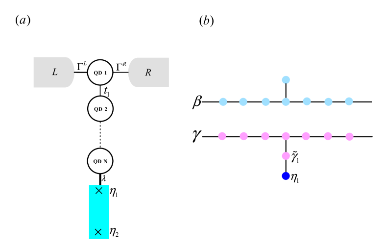
Figure 1: Sketch of a T-shaped QD system with coupled MBSs. The two MBSs are defined as $\eta_{1}$ and $\eta_{2}$, respectively. (b) Schematic of the T-shaped double-QD structure with coupled MBSs in the Majorana fermion representation.

II model

The electronic transport structure we propose to detect the MBS is illustrated in Fig.1. In such a structure, the last QD of a noninteracting T-shaped QD system is coupled to one MBS. With the current experimental technique, the T-shaped QD structure can be readily fabricated. And it is also actually possible to measure its electron transport spectrum. For example, the antiresonance phenomenon in the electron transport process has been successfully observed in an recent experimental work.Japan1 As for the realization of the MBSs, various schemes have been proposed. For instance, when a semiconductor nanowire with strong Rashba interaction is subjected to a strong magnetic field $B$ and adhere to a proximity-induced $s$-wave superconductivity, a pair of MBSs can form at the end of the nanowire,Sau ; Oreg in the case of $V_{z}=g\mu_{B}B/2>\sqrt{\Delta^{2}+\mu^{2}}$ ($\Delta$ is the superconducting order parameter and $\mu$ is the chemical potential of the nanowire).

In Fig.1, one MBS, defined by $\eta_{1}$, is assumed to be coupled to QD-$N$. Accordingly, the Hamiltonian of such a structure can be written as

$$H=H_{0}+H_{M}+H_{MD}.$$ (1)

The first term is the Hamiltonian for the T-shaped QD system with the two connected normal metallic leads, which takes the form as

$$H_{0} = \underset{\alpha k}{\sum}\varepsilon_{\alpha k}c_{\alpha k}^{\dagger}c_{\alpha k}+\sum_{j=1}^{N}\varepsilon_{j}d_{j}^{\dagger}d_{j}+\sum_{j=1}^{N-1}t_{j}d_{j}^{\dagger}d_{j+1}$$ (2)

$$+\underset{\alpha k}{\sum}V_{\alpha}d_{1}^{\dagger}c_{\alpha k}+{\mathrm{H.c.}}.$$

$c_{\alpha k}^{\dagger}$ $(c_{\alpha k})$ is an operator to create (annihilate) an electron of the continuous state $|k\rangle$ in the lead-$\alpha$ ($\alpha\in L,R$). $\varepsilon_{\alpha k}$ is the corresponding single-particle energy. $d^{{\dagger}}_{j}$ ($d_{j}$ ) is the creation (annihilation) operator of electron in QD-$j$. $\varepsilon_{j}$ denotes the electron level in the corresponding QD. $t_{j}$ denotes the tunneling between the two neighboring QDs. $V_{\alpha}$ is the tunneling element between QD-1 and lead-$\alpha$. Note that since the QD structure is noninteracting, we in this paper neglect the spin index. Next, the low-energy effective Hamiltonian for $H_{M}$ (i.e., the Majorana fermion) reads

$$H_{M}=i\epsilon_{M}\eta_{1}\eta_{2}.$$ (3)

It describes the paired MBSs generated at the ends of the nanowire and coupled to each other by an energy $\epsilon_{M}\sim e^{-l/\xi}$, with $l$ the wire length and $\xi$ the superconducting coherent length. The last term in Eq.(1) describes the tunnel coupling between QD-$N$ and the nearby MBS, which is given by

$$H_{MD} = (\lambda d_{N}-\lambda^{*}d^{\dagger}_{N})\eta_{1}.$$ (4)

$\lambda$ is the coupling coefficient between QD-$N$ and the MBS.

By applying a bias voltage $V_{b}$ between the two leads with $\mu_{L}=\varepsilon_{F}+{eV_{b}\over 2}$ and $\mu_{R}=\varepsilon_{F}-{eV_{b}\over 2}$, we can investigate the electron transport properties in the presence of Majorana fermion ($\mu_{\alpha}$ is the chemical potential of lead-$\alpha$, and $\varepsilon_{F}$ is the Fermi level in the case of $V_{b}=0$ which can be assumed to be zero). Note that in order to realize the robust MBSs, the following condition must be satisfied: the Zeeman splitting $V_{z}\gg|V_{b}|$, $\lambda$, and $\Gamma$. $\Gamma={1\over 2}(\Gamma^{L}+\Gamma^{R})$ is the QD-lead coupling with $\Gamma^{\alpha}\equiv 2\pi|V_{\alpha}|^{2}\rho$ and $\rho$ the density of states of the leads. One can notice that since the presence of MBSs, this structure is actually a three-terminal system. Thus, we have to calculate the current of lead-$L$ and lead-$R$, respectively, for completely clarifying the electron transport in this structure. With the help of the nonequilibrium Green function technique, the current in lead-$\alpha$ is expressed asMeir

$$J_{\alpha}={e\over h}\int d\omega[T_{ee}^{\alpha\alpha^{\prime}}(\omega)(f^{\alpha}_{e}-f^{\alpha^{\prime}}_{e})+T_{eh}^{\alpha\alpha}(\omega)(f^{\alpha}_{e}-f^{\alpha}_{h})].$$ (5)

In this formula, $f^{\alpha}_{e}$ and $f^{\alpha}_{h}$ are the Fermi distributions of the electron and hole in lead-$\alpha$, respectively. $T_{ee}^{\alpha\alpha^{\prime}}(\omega)={\rm Tr}[\Gamma_{e}^{\alpha}\textbf{G}^{R}\Gamma_{e}^{\alpha^{\prime}}\textbf{G}^{A}]$ and $T_{eh}^{\alpha\alpha}(\omega)={\rm Tr}[\Gamma_{e}^{\alpha}\textbf{G}^{R}\Gamma_{h}^{\alpha}\textbf{G}^{A}]$, where $\textbf{G}^{R}$ and $\textbf{G}^{A}$ are the related and advanced Green functions. Within the wide-band limit approximation, $\Gamma^{\alpha}_{e}=\Gamma^{\alpha}_{h}=\Gamma^{\alpha}$. Moreover, when the symmetric-coupling case is considered, i.e., $\Gamma^{\alpha}=\Gamma$, the two terms on the right side of Eq.(5) will be equal and $J_{L}=-J_{R}$.

In order to get the analytical form of the retarded Green function, it is necessary to switch from the Majorana fermion representation to the completely equivalent regular fermion one by defining $\eta_{1}=(f^{\dagger}+f)/\sqrt{2}$ and $\eta_{2}=i(f^{\dagger}-f)/\sqrt{2}$ with $\{f,f^{\dagger}\}=1$. Accordingly, we can write out $H_{M}$ and $H_{D}$ respectively as $H_{M}=\epsilon_{M}(f^{\dagger}f-{1\over 2})$ and

$$H_{MD}={1\over\sqrt{2}}(\lambda d_{N}-\lambda^{*}d^{\dagger}_{N})(f^{\dagger}+f).$$ (6)

Then with the equation of motion method, the matrix form of the retarded Green function can be written out, i.e.,

$$\textbf{G}^{R}(\omega)=\left[\begin{array}[]{ccccccccc}g_{1}(z)^{-1}&0&-t_{1}&0&0&0&0&\cdots&0\\ 0&\tilde{g}_{1}(z)^{-1}&0&t_{1}&0&0&0&\cdots&0\\ -t^{*}_{1}&0&g_{2}(z)^{-1}&0&-t_{2}&0&0&\cdots&0\\ 0&t^{*}_{1}&0&\tilde{g}_{2}(z)^{-1}&0&\ddots&0&\cdots&\vdots\\ 0&0&-t^{*}_{2}&0&\ddots&0&t_{N-1}&\cdots&\vdots\\ 0&0&&\ddots&0&g_{N}(z)^{-1}&0&\frac{\lambda^{*}}{\sqrt{2}}&\frac{\lambda^{*}}{\sqrt{2}}\\ \vdots&&&&t^{*}_{N-1}&0&\tilde{g}_{N}(z)^{-1}&-\frac{\lambda}{\sqrt{2}}&-\frac{\lambda}{\sqrt{2}}\\ 0&0&\cdots&0&0&\frac{\lambda}{\sqrt{2}}&-\frac{\lambda^{*}}{\sqrt{2}}&g_{M}(z)^{-1}&0\\ 0&0&0&0&\cdots&\frac{\lambda}{\sqrt{2}}&-\frac{\lambda^{*}}{\sqrt{2}}&0&\tilde{g}_{M}(z)^{-1}\end{array}\right]^{-1}.\$$ (16)

In the above equation, $g_{j}(z)^{-1}=\omega-\varepsilon_{j}+i\Gamma\delta_{j1}$ and $\tilde{g}_{j}(z)^{-1}=\omega+\varepsilon_{j}+i\Gamma\delta_{j1}$; $g_{M}(z)^{-1}=\omega-\epsilon_{M}+i0^{+}$ and $\tilde{g}_{M}(z)^{-1}=\omega+\epsilon_{M}+i0^{+}$. Via the above derivation, we can simplify the current formula in this structure as

$$J={e\over h}\int d\omega T(\omega)(f^{L}_{e}-f^{R}_{e}),$$ (17)

in which $T(\omega)=-\Gamma{\rm Im}G^{R}_{11}$.

III Numerical results and discussions

With the formulation developed in the above section, we perform the numerical calculation to investigate the electron transport properties of the T-shaped QD structure. In the context, the symmetric QD-lead coupling is considered, and temperature is fixed at $k_{B}T=0$.

First of all, we investigate the electron transport properties of the double-QD configuration with the finite coupling between QD-2 and $\eta_{1}$. The numerical results are shown in Fig.2 where $\varepsilon_{j}$ is taken to be zero. In Fig.2(a), we find that in the case of $\lambda=0$, the conductance exhibits two peaks at the points of $eV_{b}=\pm 2.0$, and at the point of $eV_{b}=0$ it becomes equal to zero. These two results are easy to understand. In the case of $\varepsilon_{j}=0$, the molecular states of the double QDs are located at the points of $\omega=\pm t_{1}$. When $eV_{b}=\pm 2.0$, the Fermi levels of the leads will coincide with the energy levels of the molecular states, respectively. On the other hand, many groups have demonstrated that such a structure provides two special transmission paths for the quantum interference. As a result, when the energy of the incident electron is the same as the energy level of the side-coupled QD, destructive quantum interference will take place, leading to the well-known Fano antiresonance effect. In the zero-bias limit, only the zero-energy electron takes part in the quantum transport, so the conductance zero comes into being.

Next, when the coupling between QD-2 and $\eta_{1}$ is incorporated, we can clearly find that the conductance peaks are first suppressed and then split. What is interesting is that in the presence of nonzero $\lambda$, the conductance at the zero-bias point shows a peak. By a further observation, we know that the conductance value at the energy zero point is exactly equal to $e^{2}/2h$. With the enhancement of such a coupling, this conductance peak is widened, leaving its peak height unchanged. For explaining this result, we should first solve the value of the conductance peak mathematically. Based on the expression of $G^{R}_{11}$ in Eq.(18), we get the analytical form of $G^{R}_{11}$ in the finite-$\lambda$ case, i.e.,

$$G^{R}_{11}=1/[\omega-\varepsilon_{1}+i\Gamma-\frac{|t_{1}|^{2}\Delta(\omega)-|t_{1}\lambda|^{2}\omega(\omega+\varepsilon_{1}+i\Gamma)}{(\omega-\varepsilon_{2})\Delta(\omega)+|t_{1}\lambda|^{2}\omega-2|\lambda|^{2}\omega^{2}(\omega+\varepsilon_{1}+i\Gamma)}],$$ (18)

where $\Delta(\omega)=[(\omega+\varepsilon_{1}+i\Gamma)(\omega+\varepsilon_{2})-|t_{1}|^{2}](\omega^{2}-\varepsilon_{M}^{2})$. Such a result shows that the nonzero $\lambda$ indeed complicates the selfenergy of $G^{R}_{11}$, hence to modify its properties. It is known that in the case of $V_{b}\rightarrow 0$, the electron transport is in the linear regime where $J={\cal G}\cdot V_{b}$. Here ${\cal G}$ is the so-called linear conductance defined by ${\cal G}_{=}{e^{2}\over h}T(\omega)|_{\omega=0}$. Surely, in such a case, the characteristic of $G^{R}_{11}$ in the region of $\omega\rightarrow 0$ plays a dominant role in contributing to the linear conductance. We can readily find that in the case of $\omega\rightarrow 0$, $G^{R}_{11}$ can be simplified, i.e.,

$$G^{R}_{11}\approx{1\over\omega+2i\Gamma}.$$ (19)

Consequently, the conductance is equal to $e^{2}\over 2h$ in the zero-bias limit.

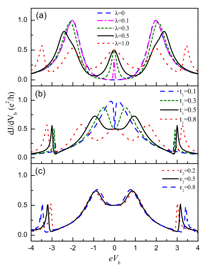
Figure 2: The conductance spectra of the T-shaped double-QD structure. The QD-lead coupling is fixed with $\Gamma={1\over 2}$. (a) The conductance as functions of $eV_{b}$ with the increase of the coupling between QD-N and $\eta_{1}$. The interdot coupling is taken to be $t_{1}=1.0$. (b) The conductance as functions changed by the decrease of the interdot coupling. $\lambda=1.0$. (c) The conductance influenced by the shift of $\varepsilon_{2}$ with $t_{1}={1\over 2}$ and $\lambda=1.0$.

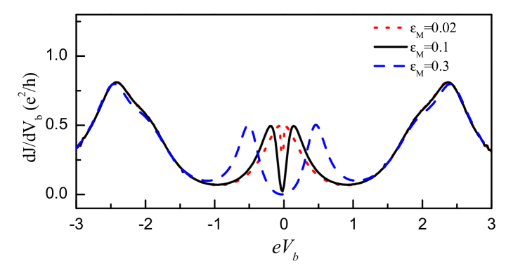
Figure 3: The conductance spectra of the T-shaped double-QD structure in the case of nonzero coupling between $\eta_{1}$ and $\eta_{2}$.

In order to further analyze the results shown in Fig.2(a), we should clarify the underlying physics mechanism in such a structure. For this purpose, we rewrite the Hamiltonian in Eq.(1) in the Majorana representation. To be specific, the two leads should be first rewritten into two semi-infinite tight-binding fermionic chains, i.e., $\sum_{k}\varepsilon_{Lk}c_{Lk}^{\dagger}c_{Lk}=\sum_{j=-\infty}^{-1}\tau(c_{j}^{\dagger}c_{j-1}+h.c.)$ and $\sum_{k}\varepsilon_{Rk}c_{Rk}^{\dagger}c_{Rk}=\sum_{j=1}^{\infty}\tau(c_{j}^{\dagger}c_{j+1}+h.c.)$ ( $\varepsilon_{\alpha k}$ and $\tau$ are confined by the relation of $\varepsilon_{\alpha k}=2\tau\cos k$). Suppose $d_{1}=c_{0}$ ($d^{\dagger}_{1}=c_{0}^{\dagger}$), i.e., the two leads with their connected QD-1 just becomes a one-dimensional chain. Next, by defining $\beta_{j}=(c^{\dagger}_{j}+c_{j})/\sqrt{2}$ and $\gamma_{j}=i(c^{\dagger}_{j}-c_{j})/\sqrt{2}$, the one-dimensional chain reduces to two decoupled Majorana chains. By the same token, the side-coupled QD can be transformed into a MBS by defining $\tilde{\beta}_{1}=(d^{\dagger}_{2}+d_{2})/\sqrt{2}$ and $\tilde{\gamma}_{1}=i(d^{\dagger}_{2}-d_{2})/\sqrt{2}$. As a consequence, one can readily find that the T-shaped double-QD structure can exactly be divided into two isolated T-shaped Majorana chains, as shown in Fig.1(b). The difference between these two chains is that there are two MBSs coupled to each other serially in the lower branch, whereas in the upper branch only one MBS is presented. For each branch, the Majorana fermion transport can be evaluated by means of the nonequilibrium Green function technique. Since the calculation is simple, we would not like to present the derivation precess. According to the calculation results, the T-shaped Majorana chain exhibits the same transport properties as the regular fermionic one. Namely, when the number of the side-coupled MBSs is odd, the transport spectra show up as an antiresonance point at the point of $\omega=0$; instead, the transport will occur resonantly if the MBS number is even. Therefore, in the T-shaped double-QD structure with the side-coupled MBSs, the transport is only contributed by the lower branch. And then, the value of the conductance is equal to $e^{2}\over 2h$ in the zero-bias limit.

Fig.2(b)-(c) show the influences of changing $t_{1}$ and $\varepsilon_{2}$ on the conductance, respectively. In Fig.2(b), we see that with the decrease of $t_{1}$, the conductance peaks in the vicinities of $eV_{b}=\pm 1.5$ enhance and shift to the zero-bias direction. However, the conductance value at the zero-bias point is robust with ${\cal G}\equiv{e^{2}\over 2h}$. Thereby, at such a point the original conductance peak vanishes and a conductance valley forms. In addition, it can be seen that during the process of decreasing $t_{1}$, the conductance peaks around the points of $eV_{b}=\pm 3.0$ disappears. These results can be understood as follows. When $t_{1}$ deceases, QD-2 tends to decouple from QD-1. In such a case, the strong coupling between QD-2 and $\eta_{1}$ will construct a new MBS which couples to QD-1 weakly. Just due to this reason, we can find that the result of $t_{1}=0.1$ is consistent with that of the small $\lambda$ in Ref.Liude, . Alternatively, in Fig.2(c), it shows that the shift of $\varepsilon_{2}$ contributes little to the change of the electron transport. This is completely opposite to the results in the absence of MBSs. We can analyze this result with the help of Eq.(19). We see that in the region of $|\omega|\rightarrow 0$, the terms related to $\varepsilon_{2}$ are ignored. This exactly means the trivial role of $\varepsilon_{2}$. Based on this result, we readily know that in the presence of MBSs, the fluctuation of QD levels can not influence the electron transport, which is helpful for the relevant experiment.

If the MBS wire is not long enough, the two MBSs will be coupled to each other. In Fig.3 we present the conductance spectra in the case of nonzero coupling between the two MBSs. It can be found that different from the results of $\epsilon_{M}=0$, the nonzero $\epsilon_{M}$ induces the appearance of the conductance dip in the zero-bias limit. When $\epsilon_{M}=0.02$, the conductance dip is relatively weak, and the conductance spectrum is consistent with that in the case of $\epsilon_{M}=0$ in principle. Next, with the increase of $\epsilon_{M}$, the conductance dip becomes apparent. Especially in the case of $\epsilon_{M}=0.3$, it exactly becomes an antiresonance with the wide antiresonance valley. This indicates that in the case of $\epsilon_{M}\neq 0$, the conductance spectrum will exhibit an antiresonance point at the zero-bias limit, similar to the zero-MBS result. However, it should be pointed out that regardless of the splitting of the conductance peak at the zero-bias case, the height of the two new conductance peaks near the point of $V_{b}=0$ is still close to $e^{2}\over 2h$. Therefore, even not in the zero mode, the effect of the QD-MBS coupling on the conductance is distinct.

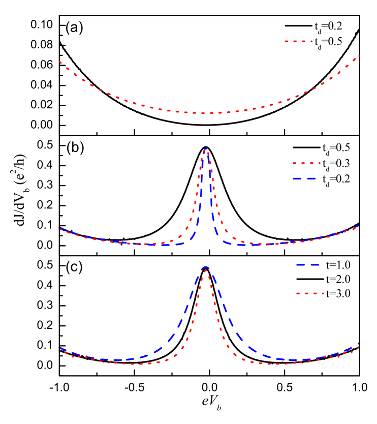
Figure 4: The influence of the Majorana zero mode on the electron transport in the double-QD case when the Majorana zero mode is mimicked by a semi-infinite chain. The structure parameters are taken as follows: (a) $t=1.0$ and $\Delta=0$; (b) $t=1.0$ and $\Delta=0.3$; (c) $t_{d}=0.5$ and $\Delta=0.3$.

In order to describe the robustness of the MBS signature in the real physical system, we next calculate the electron transport by writing the MBS into a one-dimensional semi-infinite topological superconductor.Wu1 For simplicity, we write $H_{M}$ as a semi-infinite p-wave superconducting chain, i.e., $H_{M}=-\mu\sum_{j}c^{\dagger}_{j}c_{j}+{1\over 2}\sum_{j}[tc^{\dagger}_{j}c_{j+1}+\Delta e^{i\phi}c^{\dagger}_{j}c^{\dagger}_{j+1}+h.c.]$. Meanwhile, $H_{MD}$ has its new expression: $H_{MD}=t_{d}(d^{\dagger}_{2}c_{1}+h.c.)$. By iteratively solving the end states of the semi-infinite chain, the MBS-assisted electron transport can be evaluated, and the influence of the structure parameters of $H_{M}$ can then be clarified. Fig.4 shows the numerical results with $\mu=0$. In Fig.4(a), we see that in the case of $\Delta=0$, the conductance spectra are still characterized by the apparent valleys, despite the disappearance of the antiresonance. The reason is that in such a case, the superconductor just becomes a normal electron reservoir and introduces the inelastic scattering for electron transmission, hence to weaken the antiresonance effect. But in the case of $t_{d}=0.2$, the coupling between QD-2 and the chain is relatively weak, so that the conductance minimum is almost equal to zero. On the other hand, in Fig.4(b) when $\Delta=0.3$, one conductance peak with its value equal to $e^{2}\over 2h$ appears in the conductance spectra at the zero-bias limit. The decrease of $t_{d}$ can only narrow the conductance peak but can not suppress its height. Similar results can be found in the process of increasing $t$, as shown in Fig.4(c). What is notable in Fig.4(c) is that when $t$ increases from $2.0$ to $3.0$, the conductance peak narrows more weakly compared with that of increasing $t$ from $1.0$ to $2.0$. Based on these results, it can be found that $\Delta$ and $t_{d}$ are the two key factors to adjust the MBS-assisted electron transport. At the same time, these calculations exactly verify our results in the previous paragraphs.

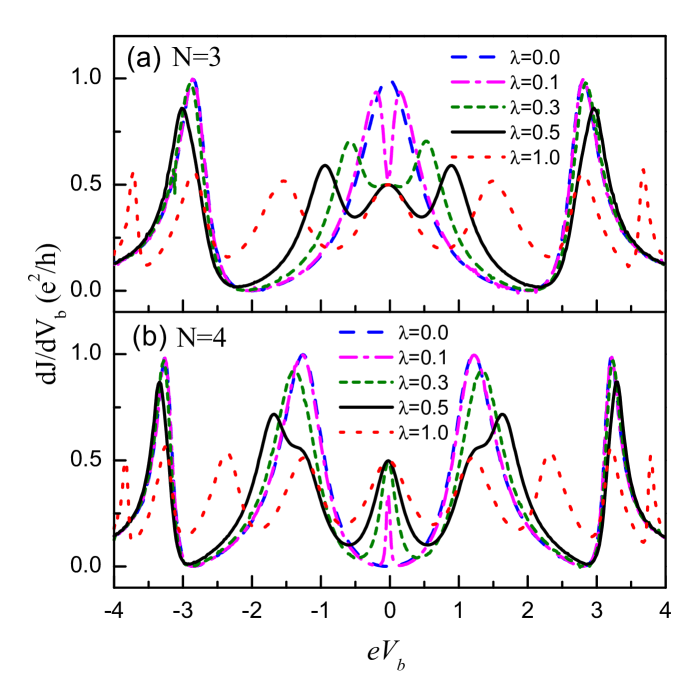
Figure 5: The conductance spectra of the T-shaped multi-QD structure. In (a) N=3, and N=4 in (b). The relevant parameters are the same as those in Fig.2.

Motivated by the results of the double-QD structure, we next investigate the multi-QD case. According to the previous works, the antiresonance is tightly related to the QD number in the T-shaped multi-QD structure. Concretely, when the QD number is even, antiresonance always appear at the zero-bias point; The resonant tunneling will be observed at such a point otherwise.Zheng ; Liuy In Fig.5 we take the cases of $N=3$ and $N=4$ to compare the electron transport properties modified by the MBS in the T-shaped multi-QD structure. From Fig.5(a), we readily find that in the case of $N=3$, the conductance is equal to $e^{2}\over h$ around the point of $eV_{b}=0$ when $\lambda=0$. When $\lambda=0.1$, despite the weak coupling between QD-3 and $\eta_{1}$, the conductance gradually decreases to $e^{2}\over 2h$ at the zero-bias point. Consequently, the conductance exhibits a valley around the zero-bias point. With the increase of $\lambda$, such a valley becomes widened. When $\lambda$ further increases to $\lambda=0.5$, the conductance magnitude is suppressed apparently, leading to the formation of the conductance peak at the zero-bias point. As for the results in Fig.5(b) where $N=4$, we see that they are similar to those in the double-QD case. The only difference is the increase of the conductance peaks. These results can be understood by following our analysis about the double-QD case. In the Majorana fermion representation, the T-shaped QD structure transforms into two isolated branches, and the side-coupled MBSs in the two branches just differ by one. Thus when the transport in one branch is resonant, the antiresonant transport certainly happens in the other. Therefore, in the low-bias limit, the conductance is certainly equal to $e^{2}\over 2h$, independent of the size of the side-coupled QD chain.

IV summary

In summary, we have introduced a Majorana zero mode to couple to the last QD of the T-shaped QD structure and then investigated the electron transport in it. After numerical calculation, we have found that the existence of the Majorana zero mode completely modifies the electron transport properties of the QD structure. For a typical structure of double QDs, the coupling between the Majorana zero mode and the side-coupled QD efficiently dissolves the antiresonance point in the conductance spectrum and induces a conductance peak to appear at the same energy position whose value is equal to $e^{2}\over 2h$. We believe that such an antiresonance-resonance transformation will more feasible to detect the MBSs, in comparison with the change of from $e^{2}\over h$ to $e^{2}\over 2h$ in the single-QD structure. Next, the influences of the MBSs on the electron transport in the multi-QD structure have been discussed. It showed that the conductance spectra always exhibit the similar conductance peaks whose values are always equal to $e^{2}\over 2h$ in the zero-bias limit, independent of the change of QD number. By transforming the QD system into the Majorana fermion representation, all the results have been well clarified. Based on all the obtained results, we propose that this structure can be a promising candidate for the detection of the MBSs.

References

- (1) G. Moore and N. Read, Nucl. Phys. B 360, 362 (1991).
- (2) N. Read and D. Green, Phys. Rev. B 61, 10267 (2000).
- (3) L. Fu and C. L. Kane, Phys. Rev. Lett. 100, 096407 (2008).
- (4) M. Sato, Y. Takahashi, and S. Fujimoto, Phys. Rev. Lett. 103, 020401 (2009).
- (5) J. D. Sau, R. M. Lutchyn, S. Tewari, and S. Das Sarma, Phys. Rev. Lett. 104, 040502 (2010).
- (6) J. Alicea, Phys. Rev. B 81, 125318 (2010).
- (7) N. B. Kopnin and M. M. Salomaa, Phys. Rev. B 44, 9667 (1991).
- (8) S. Tewari, S. Das Sarma, C. Nayak, C. Zhang, and P. Zoller, Phys. Rev. Lett. 98, 010506 (2007).
- (9) A. Y. Kitaev, Phys. Usp. 44, 131 (2001).
- (10) R. M. Lutchyn, J. D. Sau, and S. Das Sarma, Phys. Rev. Lett. 105, 077001 (2010).
- (11) Y. Oreg, G. Refael, and F. von Oppen, Phys. Rev. Lett. 105, 177002 (2010).
- (12) B. H. Wu and J. C. Cao, Phys. Rev. B 85, 085415 (2012).
- (13) C. J. Bolech and E. Demler, Phys. Rev. Lett. 98, 237002 (2007).
- (14) J. Nilsson, A. R. Akhmerov, and C. W. J. Beenakker, Phys. Rev. Lett. 101, 120403 (2008).
- (15) K. T. Law, P. A. Lee, and T. K. Ng, Phys. Rev. Lett. 103, 237001 (2009).
- (16) L. Fu and C. L. Kane, Phys. Rev. B 79, 161408 (2009).
- (17) D. E. Liu and H. U. Baranger, Phys. Rev. B 84, 201308(R) (2011).
- (18) M. Lee, J. S. Lim, and R. López, Phys. Rev. B 87, 241402(R)(2013).
- (19) Y. Cao, P. Wang, G. Xiong, M. Gong, and X. Q. Li, Phys. Rev. B 86, 115311 (2012).
- (20) B. Zocher and B. Rosenow, Phys. Rev. Lett. 111, 036802 (2013).
- (21) Z. Wang, X. Y. Hu, Q. F. Liang, and X. Hu, Phys. Rev. B 87, 214513 (2013).
- (22) X. R. Wang, Yupeng Wang, and Z. Z. Sun, Phys. Rev. B 65, 193402 (2002).
- (23) P. A. Orellana, F. Domínguez-Adame, I. Gómez, and M. L. Ladrón de Guevara, Phys. Rev. B 67, 085321 (2003).
- (24) K. Kobayashi, H. Aikawa, A. Sano, S. Katsumoto, and Y. Iye, Phys. Rev. B 70, 035319 (2004).
- (25) M. Sato, H. Aikawa, K. Kobayashi, S. Katsumoto, and Y. Iye, Phys. Rev. Lett. 95, 066801 (2005).
- (26) Y. Zheng, T. Lü, C. Zhang, and W. Su, Physica E (Amsterdam) 24, 290 (2004).
- (27) M. E. Torio, K. Hallberg, S. Flach, A. E. Miroshnichenko, and M. Titov, Eur. Phys. J. B 37, 399 (2004).
- (28) Y. Liu, Y. Zheng, W. Gong, T. Lü, Phys. Lett. A 360, 154 (2006).
- (29) S. Sasaki, H. Tamura, T. Akazaki, and T. Fujisawa Phys. Rev. Lett. 103, 266806 (2009); M. Sato, H. Aikawa, K. Kobayashi, S. Katsumoto, and Y. Iye, Phys. Rev. Lett. 95, 066801 (2005).
- (30) Y. Meir and N. S. Wingreen, Phys. Rev. Lett. 68, 2512 (1992); W. Gong, Y. Zheng, Y. Liu, and T. Lü, Phys. Rev. B 73, 245329 (2006).
- (31) A. C. Potter and P. A. Lee, Phys. Rev. Lett. 105, 227003 (2010).