The Stellar Number Density Distribution in the Local Solar Neighborhood is North-South Asymmetric
Abstract
We study the number density distribution of a sample of K and M dwarf stars, matched North and South of the Galactic plane within a distance of from the sun, using observations from the Ninth Data Release of the Sloan Digital Sky Survey. We determine distances using the photometric parallax method, and in this context systematic effects exist which could potentially impact the determination of the number density profile with height from the Galactic plane — and ultimately affect a number density North-South asymmetry. They include: (i) the calibration of the various photometric parallax relations, (ii) the ability to separate dwarfs from giants in our sample, (iii) the role of stellar population differences such as age and metallicity, (iv) the ability to determine the offset of the sun from the Galactic plane, and (v) the correction for reddening from dust in the Galactic plane, though our stars are at high Galactic latitudes. We find the various analyzed systematic effects to have a negligible impact on our observed asymmetry, and using a new and larger sample of stars we confirm and refine the earlier discovery of Widrow et al. of a significant Galactic North-South asymmetry in the stellar number density distribution.
1 Introduction
Our own Milky Way Galaxy is a spiral galaxy composed of stars, gas, dust — and a significant amount of dark matter (Gilmore et al., 1989). While matter beyond that provided by disk stars and gas is required to stabilize the Milky Way’s disk (Ostriker & Peebles, 1973), the distribution and density of that additional, apparently dark, matter is poorly known (see, e.g., Bovy & Tremaine (2012) and Garbari et al. (2012)). Disk systems are not static, and while the literature on the azimuthal and radial dynamics of spiral systems is vast, less attention has been given to studies of disk dynamics in the vertical direction.
The finding of Widrow et al. (2012) (hereafter W12) that there appears to be a significant (peak amplitude of 10%) vertical wave in the number of stars within 1 kpc of the sun is surprising and at odds with a history of models of the disk as symmetrical and static in the vertical direction. It suggests that the Galaxy is not in as close to a state of equilibrium in the vertical direction as is frequently assumed, and there may be events in the Galaxy’s recent past driving this and similar vertical waves (Gomez et al., 2013). The unexpected nature of this result makes it worth revisiting with a larger sample of stars over a larger range in Galactic longitude, while paying special attention to possible systematic effects which could affect the number counts above and below the Galactic plane.
The systematics which we explore are largely connected to our use of a photometric parallax relation to determine the distance to a star. In this the intrinsic luminosity of a main-sequence star is inferred from its color, so that its distance follows once its apparent magnitude is measured. Systematic errors also arise from the confusion of dwarfs with giants, from the existence of unresolved binaries, and from stellar population differences, particularly in age and metallicity. The stars we consider are well above the Galactic plane, but we also consider possible inadequacies in the application of corrections for reddening and extinction due to dust. To these ends we explore the dereddened colors of distant halo turnoff stars as a function of Galactic longitude as well. Finally, the location of the sun from the Galactic plane is also a systematic, in that its value impacts the precise shape of the distribution of stars with respect to the Galactic plane, though the inclusion of this effect does not reduce the significance of the asymmetry we observe. Indeed, we find that none of these effects can have a significant effect on the large (10%) asymmetry we observe in the stellar number counts North versus South.
This paper provides the background error analysis for the results of W12 and precedes the forthcoming paper (Gardner et al., in preparation), which simultaneously analyzes North-South and left-right (Humphreys et al., 2011) asymmetries and discusses their dynamical implications. In anticipation we present here the North-South asymmetry as a function of Galactic longitude as well.
2 Data Selection
We employ photometric and astrometric observations from SDSS DR9, the Ninth Data Release (DR9) of the Sloan Digital Sky Survey (SDSS) (Ahn et al., 2012). DR9 is similar to the Eighth Data Release (DR8) (Aihara et al., 2011), in that it has the same photometric imaging footprint, including a significant area of approximately 1000 square degrees over which the same Galactic longitude range is covered at moderate Galactic latitudes, avoiding the Galactic plane, of equal and opposite sign. DR9 does correct an earlier issue with the astrometry of DR8, which affected positions and proper motions of a small subset of stars with . In fact, we have used the measured proper motion of M67 to identify its stars, but that cluster is at sufficiently low that it is unaffected by this change. The photometry from DR9 is also remeasured separately from earlier SDSS data releases, and this has possible effect on the calibration of photometric parallax relations. We consider this explicitly. One further difference between DR9 and earlier SDSS imaging releases is that the DR9 release does not resolve the centers of dense clusters into individual stars as well as in earlier releases, such as in the Seventh Data Release (DR7) (Abazajian et al., 2009). These issues mean that when we test photometric parallax relations on known clusters, we find differences between different SDSS data releases. These differences, however, are demonstrably small, and in fact have negligible impact on the asymmetry.
The same telescope, instrument, and software reduction system have been used to determine both the North and South data sets, and this gives us confidence that most of the systematic effects which could affect an asymmetry in the star counts have largely cancelled out. Nevertheless, issues remain, specifically regarding inadequacies in the reddening corrections, which differ in the North and South, as well as large-scale calibration offset differences, both of which could mimic stellar population differences. We analyze these in more detail than could be done in the limited space of W12.
To minimize obfuscation from dust, we consider high Galactic latitudes, so that the viewing is well out of the Galactic plane. We thus assume that all of the stars we select are beyond the dust, which is thought to lie at (Marshall et al., 2006) — this study is for only, but Fig. 19 of Berry et al. (2012) reveals that the dust scale height actually increases as one goes to the Galactic center, making the assessment of Marshall et al. (2006) a conservative one for our analysis. Throughout we convert from the observed apparent magnitudes in the SDSS filters to “dereddened” ones, denoted by a “0” subscript, using the extinction maps of Schlegel et al. (1998). The dust maps depend on the Galactic longitude and latitude and are rather different in the North and South, though the effects of dust are substantially reduced at the higher latitudes which we employ here. Moreover, for our stars, which are predominately late K and M dwarfs, the vast majority of the region in both the north and south has extinction . Specifically, using the Schlegel et al. (1998) maps, we note that less than 1% and 5.6% of the area in the North and South, respectively, has .
We have recently studied (W12) a data set selected as per the following criteria: namely, stars with Galactic coordinates with and that also reside within a perpendicular distance of from the line extending directly up and down from the sun in the vertical coordinate . Limiting the -band magnitude such that and yields a data set of some 300,000 (0.3 M) stars. The study of this data set yields a significant North-South asymmetry which has the appearance of a wavelike perturbation. In this paper we select a similar but non-identical data set, to investigate whether we can confirm the North-South asymmetry observed in our earlier data set. Moreover, if an asymmetry is present and is indeed the result of a perturbation, it is possible that it is localized to particular Galactic longitudes in the neighborhood of the sun. We will pursue this possibility explicitly in Gardner et al. (in preparation), and this predicates the use of a data set with broader coverage in . We thus select the stars of our present study under slightly broader criteria. The selected stars from SDSS DR9 satisfy the constraints and , with brightness but without saturation yielding a sample of some stars. The selection in is shown in Fig. 1. Restricting to as per W12 yields a data set of some stars, comprised of late K and M dwarfs (Covey et al., 2007). We select , magnitude, , , and colors for each star. Note that there is no cut on the distance from the sun imposed explicitly here as there was in W12. For our asymmetry analysis as a function of Galactic longitude, we consider a data set with , a sample of some 1.98M stars, comprised of K and M dwarfs (Covey et al., 2007).
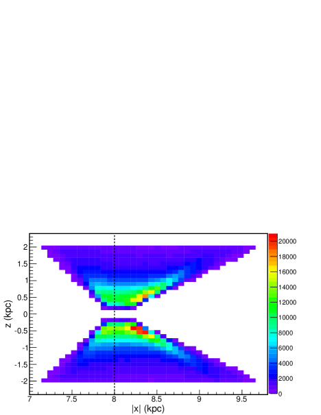
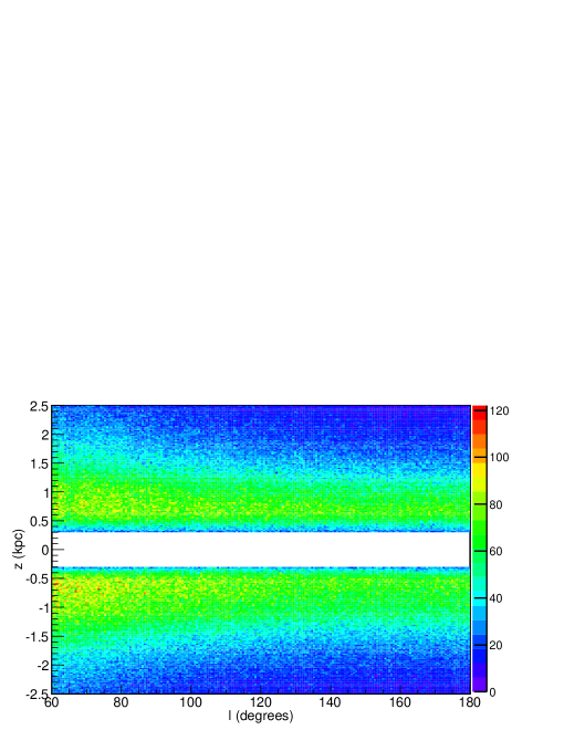
The covered region in and is shown in Fig. 2; note that this range is also manifestly North-South symmetric and extends to kpc. In comparison, the fits of W12 extend to kpc. We use band observations to assess the apparent magnitude of our stars because for the red stars we employ this band offers the greatest signal-to-noise ratio for the range of types of stars, which are K and M dwarfs, in our sample. From these inputs we estimate the distance to each star, albeit with systematic and statistical uncertainties, as we detail in the next section.
3 Photometric Parallax Stellar Distances
The color of a main-sequence star can be used to determine its absolute magnitude through a photometric parallax relation. Although typical random errors for stars at in the SDSS catalog are 7%, after averaging together large numbers of measurements we can reduce the color errors for stars as faint as this magnitude to the level of the systematic error of 1.5% (Padmanabhan et al., 2008) or below. Combining statistical and systematic errors in quadrature, the associated colors are thus determined to within 3% for even the faintest objects.
We determine the distance to a star in our sample of stars from DR9 using relations constructed using the stars imaged in SDSS DR7, such as those of Jurić et al. (2008), in color, and of Ivezić et al. (2008), in color, respectively. To employ the photometric parallax method we have made a number of implicit assumptions, whose assessment ultimately lead to estimates of systematic errors. They concern i) the identification of the stars in the survey, i.e., whether they are single, main-sequence stars or not, ii) the neglect of unmeasured properties such as stellar metallicity or age on the determined distance, iii) the role of dust in the context of our use of the Schlegel et al. (1998) maps, and iv) large-scale calibration issues between non-contiguously connected regions of the sky. We will consider each of these possibilities, and in each case we provide detailed, observational tests of our procedures.
To begin with, however, we test and calibrate the photometric parallax relations we employ by applying them to the study of stellar clusters at known distance. Of these, we choose clusters out of the Galactic plane containing stars of comparable color and metallicity to those in our data set. These criteria severely limit the number of clusters we can employ; indeed, the clusters M67 (NGC 2682) and NGC 2420 turn out to be the only suitable candidates. Both clusters have been imaged (once) by the SDSS and were released in both DR7 and DR9. The image processing was similar but distinct in the two cases. The primary difference was that the processing in DR7 ran with a longer timeout, so that it resolved stars appearing deeper towards the centers of these clusters than in DR9 (Aihara et al., 2011). The final photometric calibrations of DR7 and DR9 were performed separately using methods described in Padmanabhan et al. (2008). We calibrate the photometric parallax relations we use with cluster data from DR7. Note that the relations used in this paper and in W12 differ in that different procedures to assess cluster membership were employed in the two cases. Here we advocate a more refined procedure, as we shall describe. We also evaluate the impact of the shift from the use of DR7 to DR9 reductions quantitatively.
We employ photometric parallax relations devised by Jurić et al. (2008) in color and by Ivezić et al. (2008) in color. The analyses of Jurić et al. (2008) and Ivezić et al. (2008) are based on main sequence fitting to a set of cluster fiducials covering a large range in color. In W12 we used a different zeroth coefficient in each case in order to confront the literature distance to M67 successfully. We have refined that adjustment in our current work. For color, we begin with the “bright” relation of Jurić et al. (2008), valid over the color range , include a correction for the metallicity, and adjust the constant term in order to confront the cluster distances we have noted. In W12 we employed
| (1) | |||||
for the absolute magnitude , noting a metallicity correction (Ivezić et al., 2008), with in dex characterizing the metallicity. We assume a universal in our analysis of K and M dwarf field stars; however, as we proceed out of the Galactic plane in we expect the fraction of stars (i.e. a thick disk population) with a metallicity content of to increase. If , the assessed distance would be off by some 200 pc, or some 20% on 1 kpc. Our assessed distance error at any given height is a small fraction of this. This additional systematic error in distance for low-metal, thick-disk stars could potentially impact the location of the second peak in our asymmetry somewhat. We note, then, that the final constant term in color for these stars evaluates to some 0.50 mag less than that employed in Jurić et al. (2008). Although this may seem like a large offset it will not turn out to be so. One reason for this is that the stars used to calibrate Jurić et al. (2008) and Ivezić et al. (2008) were much bluer and essentially disjoint from the red stars used to calibrate our version of their photometric parallax relations. Interested readers can find more sophisticated M-dwarf photometric parallax relations in Bochanski et al. (2013). In performing the current analysis, we realized that the large offset we found was driven by our simple assessment of cluster membership in M67 and NGC 2420, which we amend here. In the current paper we employ a constant term of 3.2 in Eq. (1), which is just that of Jurić et al. (2008), though we allow for a metallicity correction of as well, unlike that work. Note that both the current analysis and that of W12 were adjusted to yield the literature distances to the clusters; the play of some 20% in the distance assessments is a consequence of the manner in which we deduced cluster membership — it is removed once the membership criteria are sharpened. Thus we investigate these issues in careful detail. The relation of Ivezić et al. (2008), for , comes from confronting DR7 SDSS globular cluster data with , and the shape of the extension to redder colors was developed from the “bright” relation of Jurić et al. (2008), over the color range . For color, we start with the relation of Ivezić et al. (2008) and adjust the constant term in order to confront the cluster distances we have noted. In W12 we employed
| (2) | |||||
where we used precisely the same metallicity correction in both color bands. We note that our constant term for these stars is some 0.66 mag less than that employed in Ivezić et al. (2008). This shift, too, is a consequence of our assessment of cluster membership. In the current paper we employ a constant of -.50, which is 0.06 mag greater than the constant in Ivezić et al. (2008). Finally, we estimate the distance (in parsecs) to a star with intrinsic magnitude and apparent magnitude via the standard relation . The analysis of Jurić et al. (2008) has been used to study the stars of the local solar neighborhood, particularly to the end of determining the height of the sun with respect to the Galactic plane. In comparing the stars selected for our asymmetry analysis with those of that study, our sample is not as red in color so that it does not go as close to the Galactic plane. Moreover, our estimated offset of the intrinsic luminosity, as per the reference distance to stars of a more limited color range, also pushes our stars somewhat farther away.
In what follows we reexamine these photometric parallax relations in detail using the observations of main sequence K and M dwarf stars in our two chosen reference clusters, paying careful attention to cluster membership and other systematic effects. We calibrate the photometric parallax relations we use with cluster data from DR7. We then employ our calibrated relations to study the distance to the stars from the same clusters in the DR9 data set, to examine whether any additional adjustments of the photometric parallax relations are necessary. We wish to realize the sharpest assessment of the photometric distance possible, making analysis choices driven by data independent of our asymmetry sample in order to realize an accurate assessment of its shape.
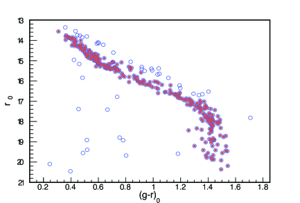
We begin with the cluster M67, for which proper motion information is available (and which we did not exploit in W12). Figure 3 shows the proper motion of stars in and around the field of M67. There are two distinct loci, that of stars in M67 itself and that of a somewhat broader set of stars clearly separated from M67. These are Milky Way field stars. The preliminary membership cut was based on an empirical look at the one-dimensional histograms of in each coordinate ( and ). The cut was slightly refined by displaying candidate members in a color-magnitude diagram and finding a reasonably small number of outliers. We have made the following proper motion cuts: and . No objects with a proper motion error greater than 5 in either coordinate are included. A histogram of proper-motion errors shows a modal value of about 2.5 . Figure 4 shows a () color-magnitude diagram (CMD) of DR7 stars near the position of the cluster M67 which have proper motions consistent with it. A cursory glance at Fig. 3 shows that the Milky Way field in this direction has an average proper motion significantly offset from the M67 average proper motion, so that this procedure removes most field stars, but there is some overlap.
While the proper motion cut significantly decreases outliers, there remain several field stars which stand out in the CMD. Also, there is a clear sequence of unresolved, roughly equal-mass binaries sitting approximately 0.7 mag above the main sequence. These, as well as the obvious field stars, are separated with simple diagonal cuts and are indicated with open symbols. The filled circles represent our “cleaned” sample used to calibrate our photometric parallax relations. Roughly half of all stars are in binaries, as borne out by explicit study of the M67 cluster (Fan et al., 1996). However, since the luminosity of a main-sequence star scales as its mass raised to the power , the distance to a sufficiently unequal-mass binary can nevertheless be reasonably evaluated through use of a photometric parallax relation — upon assuming that the heavy companion were alone present. A star which is 2.5 times brighter than another is approximately 1.0 less than it in magnitude; thus we see that evaluating the magnitude of a binary of main-sequence stars by replacing it with the heavier star of them yields magnitude shifts of 0.75, 0.57, 0.41, and 0.28 for a binary with stars in a mass ratio of 1.0, 0.9, 0.8, and 0.7, respectively. The appearance of binaries smears the locus of points in the connection of color to intrinsic luminosity and thus limits the precision to which we can assess the distance — this will be reflected in the scatter of distances we determine to the stars in the cluster, which we will assess as a statistical, or random, error. Studies of the mass-ratio distribution shows that binaries occur more frequently in relatively close mass pairs, both in the M67 cluster, noting Fig. 14 of Fan et al. (1996), and for solar-like stars in the Milky-Way field, noting Fig. 16 of Raghavan et al. (2010). The presence of such like-mass binaries smear the color-luminosity relation the most and thus, from the perspective of distance assessment, are the most problematic; however, from visual inspection of Fig. 4 we see that they are only some 10% of our cluster stars. We identify 27 of such objects in DR7, which we presume are binaries with mass ratios of 0.9 or greater; this number compares closely to the some 30 stars noted in Fig. 14 of Fan et al. (1996). Although equal-mass binaries must also be present in our field stars, possibly with equal probability, we have omitted correcting for a fraction of these objects in our calibration of our photometric parallax relation because we believe it best to sharpen the distance determination of the preponderance of stars in our sample. We note that this cleaning procedure was not effected in the calibration used in W12, so that we can test the impact of this choice through the comparison of our results with those of W12. Let us remark in advance that we observe no changes which would be predicated by this.
Figure 5 shows a () diagram after applying the photometric parallax relation of Eq. (2) and employing (An et al., 2008b) for the cluster. We also show the diagram in Fig. 6, which results from using the distance relation of Eq. (1). As for the reference distance to this cluster, we note the recent compilation of Schlesinger et al. (2012); assuming the results therein are independent, we make an error-weighted average, assuming the errors are independent, to find . We use this result in what follows, though we note by comparison the distance obtained from the use of empirically calibrated (theoretical) isochrone models is kpc (An et al., 2007a).
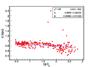
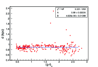
Ideally the determined photometric distance to a cluster should be independent of the employed color; the extent to which this is practically so is a test of the photometric parallax relation. In Fig. 7 we probe the color-distance relationship for M67; we show three panels, the first employing Eq. (2) to yield (in kpc), which we denote as . Fitting a linear polynomial in color to these results, for , yields a small correction amounting largely to a slope adjustment. Specifically we note the corrected distance is
| (3) |
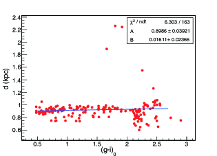
and the impact of the use of this correction is shown in the second panel. Our experience with the fits indicated that the use of a linear correction was sufficient. The third panel shows the result of applying Eqs. (2) and (3) to the DR9 (rather than the DR7) sample. It is apparent that the small correction gives a significantly better fit, and it is also apparent that the SDSS calibration of the DR9 sample is close enough to the DR7 sample that the same photometric parallax relations (with linear slope correction) may be used for both DR7 and DR9. We now proceed to determine how precisely we can assess the cluster distance.
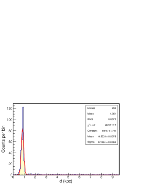
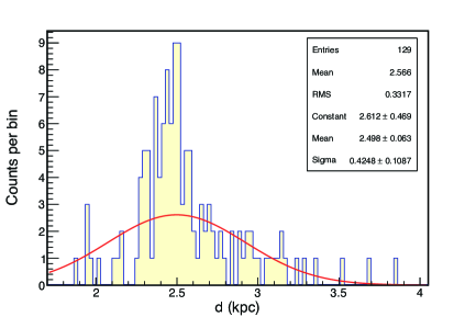
The upper left panel of Fig. 8 shows the DR7 data for the M67 cluster with only the proper motion cut applied. The upper right panel shows the same field with the unresolved binaries removed, as per the “cleaning” procedure we have described, noting the changed scale on the x-axis. The lower panel is the DR9 version of the upper right panel, i.e., the binaries have been removed via a similar procedure and the same proper motion cut has been applied. Each panel shows both a histogram of the distances to the stars in the cluster as well as the results of a Gaussian fit. The fit parameters are listed in small boxes at the upper right of each panel. We list from the top down: the number of stars, the histogram mean and root-mean-square (RMS), as well as the information for the Gaussian fit, for which . That is, we show the per degree of freedom, as well as the fit parameters, namely, a constant (), mean (), and sigma (). The two most relevant parameters to compare are the histogram RMS with the sigma from the Gaussian fit. These parameters should agree in the limit of a large number of points if the data set is indeed normally distributed 111http://root.cern.ch. In particular, when a data set has many outliers, the histogram RMS width may be very different from the Gaussian width. For instance, in the upper left panel, the histogram RMS is , whereas is only . After cleaning, the histogram RMS becomes , whereas becomes — the difference has shrunk from a factor of eight to a factor of two. Looking at the DR9 sample, after a similar cleaning procedure has been applied, the RMS is , whereas is , yielding a comparison somewhat worse than the fit to the DR7 data. We are not concerned by this because the DR9 data set has only 65% as many stars as the DR7 sample. We regard the difference between the histogram RMS and the Gaussian sigma as an estimate of systematic error, reflective of the presence of non-cluster members, whereas sigma itself provides a statistical error estimate. We combine these two types of error in quadrature, using the results of the upper right panel of Fig. 8, to determine , reproducing the Schlesinger et al. (2012) distance by construction, to find a total cluster distance error of about 0.11 kpc. For the DR9 set, kpc for a total error of 0.16 kpc; the two data sets are clearly compatible. The latter result thus also compares favorably with the average literature value we have determined from Schlesinger et al. (2012), namely, kpc. This gives us confidence that we can employ our DR7-tuned photometric parallax relations on the DR9 data set. Note, too, we are able to assess the cluster distance to within . Noting once again the upper right panel of Fig. 8, we can translate the statistical error in the distance to the cluster to a typical error in the distance to a star by multiplying 0.066 by the square root of the number of cluster members, to yield an error of about 0.11 kpc. Consequently, we claim that we can assess the distance to a star in M67 to as well.
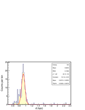
We now turn to the analysis of the cluster NGC 2420, for which we employ a metallicity of (Anthony-Twarog et al., 2006; Lee et al., 2008), though other determinations have yielded a range of metallicities (Lee et al., 2008). Figure 9 shows a CMD of members of the cluster NGC2420 from DR9, which have further been culled by only keeping objects with SDSS heliocentric radial velocities compatible with the radial velocity of the cluster, (Lee et al., 2008), though Lee et al. (2008) note previous radial velocities measurements ranging from . We note that the systematic proper motion of NGC 2420 and that of nearby Galactic field stars do not differ significantly, so that we cannot use the method we employed for M67 to isolate cluster members here. Velocities from SDSS stellar spectra typically have errors of , so that we do not restrict the cluster membership based on the error in the determined radial velocity and demand only that the velocity itself fall within the interval . Since our ability to determine cluster membership is less crisp in this case, we do not try to refine our distance assessment further. Rather, we wish only to apply our present procedure to the stars of NGC2420, as an additional test. We show in Fig. 10 the photometric parallax relation for NGC2420 stars with (small filled circles) and without (open circles) the slope correction derived from M67. The slope correction lessens the variations in the computed distance with color slightly. In Fig. 11 we compare the Gaussian fit to the histogram of NGC2420 distances. We apply the same procedure we used previously for M67 to determine the systematic and statistical distance errors, finding kpc for a total distance error of kpc. An error-weighted average of the distances given in Schlesinger et al. (2012), assuming the errors are independent, yields kpc. The determinations compare favorably, though the width of the Gaussian fit in this case is much broader than it was for the M67 cluster. This could be reflective of the presence of a range of metallicities within the cluster, giving a basis for the range of metallicities found in studies of selected stars (Lee et al., 2008).
We now repeat our -based analyses with one based on color and its associated photometric parallax of Eq. (1), after Jurić et al. (2008). By so doing we wish to show that our assessment of systematic errors is independent of the particular choice of photometric parallax relation. This is also crucial for our ultimate application of these refined relations to the stars of our asymmetry analysis, for we wish to demonstrate that the results which emerge there are also independent of the photometric relation chosen. For this to be a sensitive test, the two relations must be similarly well calibrated. Thus we have repeated the analysis depicted in Fig. 7 using the photometric parallax relation in color. The determined linear correction in color turns out to be slightly larger in this case, yielding a corrected distance , namely,
| (4) |
We have also confirmed that the same correction applied to the distances to the stars in the DR9 data set also yields a reasonably flat distance relation with color, rather comparable to that shown in the third panel of Fig. 7 for color. While there are star-by-star differences between DR7 and DR9, the corrected photometric parallax relation remains flat — no additional adjustments are needed, and we do not make any. We have made Gaussian fits of the distances to M67, mirroring Fig. 8 for color. For DR7 we obtain , whereas for DR9 we find , very comparable to the results. We have also studied the NGC2420 distances before and after applying the M67-derived correction to the NGC2420 candidate members after the radial velocity cut has been applied. In this case the distance refinement yields at best a modest improvement. Finally, the DR9 NGC2420 sample, refined by the radial velocity cut we have described, is fit, which yields . This distance is also compatible with the reference distance to this cluster.
We conclude that our distance estimates, as well as their precision, are not sensitive to the specific photometric parallax relation we choose. We demonstrate that we are able to recover statistical distance errors for the cluster for which we have the best membership information. Moreover, we are able to assess the systematic errors incurred quantitatively by our assumption of cluster membership and find that they are no larger than our assessed statistical error. We have employed both parallax relations in the analyses which follow, and find no marked differences, though we focus on the results determined through use of the color relation in what follows. We used a relation in W12; a comparison of the detailed calibrations reveal, however, that the correction required to yield a M67 cluster distance independent of color is smaller in the case of the relation. Moreover, we find that we can study a somewhat larger interval in in the case. Thus we favor this choice in what follows.
3.1 Stellar Identification
Although the great preponderance of the stars in our sample are K- and M-type main-sequence stars, it is possible that giants can appear in our sample as well. Moreover, although their distances are reasonably determined by treating them as single, resolved objects, near-equal-mass unresolved binaries can also be present — the distances to the latter, as we have noted, are not well-treated by this approximation. We consider each of these possibilities in turn.
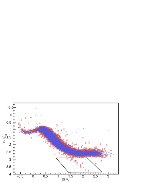
Our selection is numerically dominated by faint-end-magnitude stars; this ensures that giants can only play a small role in our sample. Exploiting the full multi-band nature of the SDSS data also permits us to make an explicit numerical bound on their appearance. Figure 12, similar to Fig. 10 of Yanny et al. (2009b), reveals the extent to which giants appear. Giants are visible in color-color space as a small diagonal tail running from to . Their numbers are completely swamped by dwarf stars; specifically for the band selection , we note that there are only some 30 giants in comparison to roughly 70,000 main-sequence stars, for a pollution of only some . Only a fraction of the few giants which do appear in Fig. 12 can appear in the sample which we analyze in this paper. Consequently we conclude that giants have no impact on either the number count asymmetries of W12 or on the asymmetries we present here. Fig. 12 also splits the stars into solid circle (blue) () and open circle (red) () subsamples. The distributions of these two samples in color-color space, while not identical, lie on top of each other, suggesting there is no gross stellar population difference, i.e., from either metallicity or age, in these two sub-populations. We return to this point in the next section.
We now turn to the possibility of unresolved, equal-mass binaries in our sample. Figure 4 shows a locus of stars shifted about 0.7 mag brighter than the single star locus for the cluster M67; it seems that some 10% of the stars are near equal mass unresolved binaries (Fan et al., 1996). In the general field, we note the study of solar-like stars using data from Hipparcos (Raghavan et al., 2010): Fig. 16 of that reference shows that 17 of 110 binaries have a mass ratio of 0.9 or greater, which is consistent within statistics with our study of M67. Even though we do not correct for this effect in the field, there is nothing different about the way these objects affect apparent star magnitudes above or below the plane, and again, as with the contamination by giants, unresolved binaries cannot not alter the asymmetry results of W12 significantly.
3.2 Role of Unmeasured Properties: Metallicity and Age Effects
How do unmeasured properties such as age and metallicity impact the assessed distances to our stars? Stellar age is a particularly straightforward issue for us, since we are dealing nearly exclusively with stars (K and M dwarfs) which have not yet begun to evolve off the main sequence. A spread in the ages of these stars will not have a significant effect on their colors until they do so. Moreover, the impact of very young stars is also not an issue. The minimum height above the plane for our stars is no less than 300 pc, so that we are also confident that the vast majority of our stars () are already on the main sequence and have standard color-magnitude relations for main sequence K and M stars (Jurić et al., 2008). T Tauri stars and other young stars which may still be on their descending Hayashi track to the main sequence are restricted to distances much closer to the plane. In particular, the scale height of molecular gas, where essentially all stars are born is only 74 pc (Dame et al., 1987). The role of metallicity is a more difficult issue. Attempts to determine metallicity from photometry only (Ivezić et al., 2008) almost invariably rely on the determination of -band-connected colors because such colors are the most sensitive (for SDSS filters) to the presence or absence of the line-blanketing effects of UV atomic metal transitions. While we have access to the -band magnitudes and colors for our stars, we do not have sufficient precision in the band to develop a sufficiently accurate photometric proxy for the metallicity. Nevertheless, our Fig. 12, with its closely overlapping North and South dwarf stellar loci, crudely demonstrates the absence of a strong shift in the average metallicity of the two samples. Although vertical and radial gradients in the metallicity are known (Chen et al., 2011), the existence of possible north-south differences have not been documented. Certainly our Fig. 12 offers a simple probe of this issue and suggests that it is unimportant, allowing us to set it aside.
3.3 Testing Dust Corrections
A remaining systematic effect concerns the possibility of inadequately estimated reddening differences between the North and South. While the Schlegel et al. (1998) dust maps have been shown, using photometry and CMD histograms, to be very accurate (Schlafly et al., 2010), especially for higher latitude () sight-lines, there remains their finding, which is affirmed with a separate analysis using stars with SEGUE spectra (Schlafly and Finkbeiner, 2011), that the stars in the South, working in color and using a very large scale average, appear to be about 0.02 mag redder than the stars in the North. This result is based on the average colors of blue turn-off stars. The difference in color is smaller by a factor of three.
There are three possible explanations for the observed color difference. First, there may be a global calibration error in the photometry within the SDSS DR7 (and DR8) releases, which the study of Schlafly et al. (2010) supports, though this, noting Table 4 of Schlafly et al. (2010), does not seem to capture the complete effect. However, the differences in area in the two studies implies that the conclusions of Schlafly and Finkbeiner (2011) need not hold for the photometric study (Schlafly et al., 2010). An offset in the -band magnitude scale is the most likely because the blue-tip stars in color are relatively unaffected. Maintaining absolute calibrations to better than 1% across very large areas, especially those which are only nominally contiguous, as it is here with different regions connected only by narrow strips running through the Galactic plane, is an extremely difficult task, subject to many subtle problems. A recent analysis by Betoule et al. (2013) re-examines the large scale calibration of the SDSS with an effort toward improving Type I supernovae (standard candle) distances and finds that there are indeed systematic drifts in the SDSS calibration of some filters at the level of 1% to 2% over 100∘ scales. Thus we regard it as very possible that such a large-scale calibration drift exists in the band between the North and South. A second way to explain a global color difference would be a reddening map anomaly. All our colors and magnitudes are corrected for reddening based on Schlegel et al. (1998). We regard a problem with the reddening maps to be unlikely, as we discuss below, but we cannot completely rule out this possibility. A third way to have a global color difference would be through an actual stellar population difference, namely, that the distribution of stellar metallicity is different above and below the Galactic plane. This, too, we think is unlikely, and we discuss it further later.
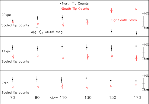
In order to select among the possibilities, we divide the “blue-tip” stars (turn-off stars of spectral type F extending to the halo of the Milky Way), in our survey region into six 20∘ segments in Galactic . We plot the color histograms of these blue-tip stars in three magnitude bins, namely , and , and measure the central color and peak heights of each histogram in the north and south samples separately. Since Schlafly et al. (2010) uses CMDs for their analysis of blue-tip stars, we adopt the same analysis for consistency. The results of this analysis are reported in Table 1, and the number count studies and color offsets are also summarized in Fig. 13. Table 1 presents peak turnoff color for star subsets, namely for and the indicated range with restricted to the range given in brackets. The numbers in parentheses indicate the total star counts in the central bin. Note that the number counts of blue-tip stars in each bin should roughly match in the north and south (within Poisson errors), provided the halo is fairly smooth. Within Poisson statistics, only two bins (in boldface) are markedly discrepant — and we will find that they correspond to the angular location and distance of the turnoff stars in the Sagittarius stream.
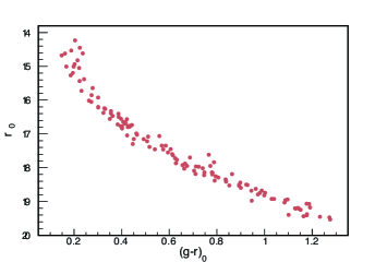
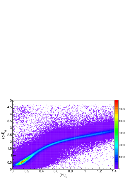
Generally Fig. 13 and Table 1 show that the number of turn-off stars tends to fall more or less smoothly for a fixed band of as increases, i.e., as one looks away from the Galactic center. There is one pair of bins in the South, however, with and , which is strikingly inconsistent with that trend. In this case the difference in the number counts in matching bins North and South are several times the square root of the counts in the corresponding bins — suggesting the presence of a structure. In fact these bins in the South are contaminated by Sagittarius stream stars, as can be seen by an examination of Fig. 9 of Yanny et al. (2009a), which clearly shows the Sagittarius stream passing through this range. The implied distances to the blue-tip stars, that is, kpc, closely matches that of the distance to the Sagittarius stream stars. Aside from this particular structure present in the South, the relative numbers of blue-tip stars in the North and South are fairly closely matched. We also note that the average colors of the South blue tip stars are systematically a couple of percent redder than the corresponding bins in the North, and these differences persist across four of the 20∘ longitude bins and three different magnitude bins, the latter corresponding to three different distance bins ranging from some 5 to 25 kpc from the sun. This persistent color difference, which is just what Schlafly et al. (2010) found, argues strongly against the existence of a localized stellar population difference, or a localized “rogue dust cloud,” in either just the North or the South, but rather suggests a global calibration difference. In support of this we show in Fig. 14 the comparison of and for stars in our sample. The tight central locus of Fig. 14 which appears without sharp bends, shows that one color may be substituted for the other without large shifts of estimated (photometric parallax) distances. This in itself argues against the possibilities of rogue population or reddening differences. Note that even with this global calibration difference, the star counts made in the North in comparison to those made in the South are not really affected because we see the same asymmetries whether we use the or the photometric parallax relation. We have shown, too, by exploring photometric parallax relations in two correlated color ranges, and , that our distance estimates are independent of the filters used.
4 The North-South Asymmetry
We now proceed to analyze our larger sample in the spirit of W12, to determine the vertical distribution of the stars and finally the North-South asymmetry they possess with respect to the center of the Galactic plane. To do this, we must first determine the appropriate saturation and color cuts. We then construct a selection function in order to estimate the stellar number density as a function of vertical displacement from the sun, given that our stellar sample is restricted to a limited window in and . We note that with suitable color cuts the selection function is determined by purely geometric factors. Finally, we fit our inferred “true” vertical distribution of stars to a theoretical form in order to determine the location of the sun with respect to the Galactic plane. With this in hand we can finally determine the North-South asymmetry about the Galactic plane — and we have sufficient statistics to analyze its variation with Galactic longitude as well.
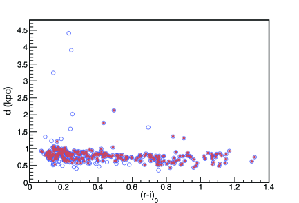
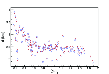
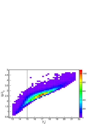
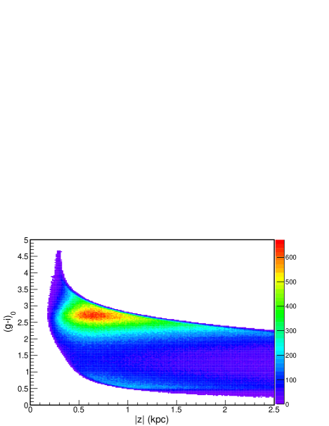
The SDSS data are affected by a selection on the bright end — most objects are saturated if . In order to make our saturation limit more uniform in color, we apply a slightly fainter saturation cut (though we used in W12). Its intended effect is to remove any systematics due to saturation in our asymmetry analysis. Fig. 15 shows that we may remove stars with — this improves the completeness of the sample on the near end, without significantly losing statistical significance. Fig. 16 shows how the particular colors of the stars relate to their vertical distances, where we impose and compute distances as per Eq. (3). The shape of the region is determined by our window on ; a judicious choice of color interval opens a vertical window on which is not limited by our finite range of . We note, e.g., that if we choose , our sample is complete on the interval . In DR9, there are some 794,500 stars which satisfy all our cuts. The selection function is determined by geometry. Since we bin the photometric data with vertical height, the selection function is the effective volume, bin by bin, associated with the observed stars. That is, if the center of a vertical bin is at , then the selection function for our North-South symmetric data sample is
| (5) |
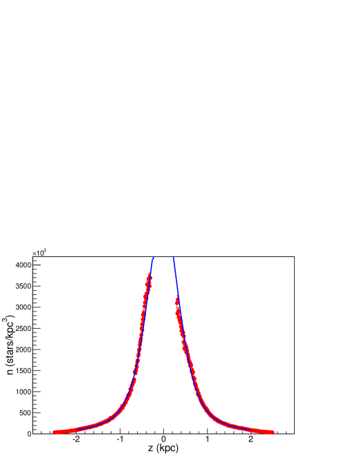
where is the bin width in kpc, noting and are in radians. Finally we fit the function determined by , where is the number of stars we observe in a vertical bin centered on . We adopt the same standard Galaxy thin and thick disk model form used in W12,
| (6) |
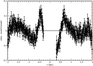
and show the result in Fig. 17, which displays the stellar number density as a function of distance. Already here we see that the deviations of the counts from the best-fit model change sign under ; i.e., they are odd under parity. This is further highlighted in Fig. 18. We have 600 bins over the region , so that . The fit is over the region with , yielding , , , , , and . Figures 17 and 18 update Fig. 1 in W12. The quality of our fit is markedly better than in W12, due to an improved calibration and saturation-cut choices, though we still reject a North-South symmetric model for . The results of Figs. 17 and 18 evince a North-South asymmetry, strongly confirming the results of W12.
We construct a North-South asymmetry by comparing star counts North and South directly. If we compare, e.g., the raw counts as a function of the vertical displacement from the sun’s location, we define
| (7) |
This quantity is shown in Fig. 19. Ultimately, however, we would like to determine the North-South asymmetry in terms of the effective stellar number density as a function of the vertical displacement from the Galactic plane. We realize this in two steps. First, we plot the raw asymmetry in terms of as shown in Fig. 19. We then include the selection function as well, in order to compute the asymmetry in terms of the effective number density, namely,
| (8) |
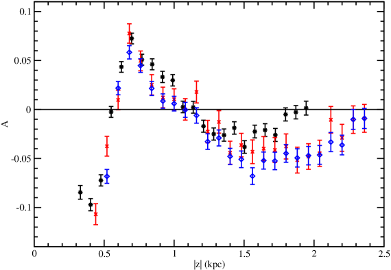
We use as per our earlier fit. The North-South asymmetry is visible in the original star number counts, and the refinements we have included in Eq. (8) impact its precise shape but not its significance. At this point it is appropriate to revisit the various systematic effects we have studied earlier in the paper and explore their impact on the asymmetry. Specifically, we consider the role of , the impact of our tune of the photometric parallax relation from the fit to M67 data, Eq. 3, and finally the impact of a possible 2% calibration error in the band, either North or South. The asymmetries which result from these changes are illustrated in Fig. 20. In all cases the resulting asymmetry is still significantly non-zero. However, the impact of the change in and in the tilt and offset of the photometric parallax relation away from the optimal values determined in our fits yield significant changes in the shape of our asymmetry. The impact of the possible 2% calibration errors is, in contrast, much smaller.
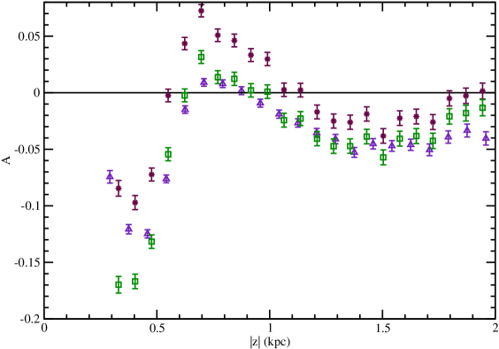
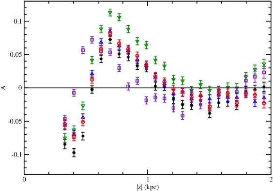
In Fig. 21 we compare the asymmetry computed using different color bins; the window on the vertical coordinate for each color band is limited by the saturation and faintness limits on in each case, noting, e.g., Fig. 16 for color. We show the asymmetries for three different bins on color, namely, , , and . The different asymmetries are reasonably similar where they all coexist. We also compare these results with an asymmetry determined from distances computed using color, namely Eq. (4). Choosing a sample with , we note as per Fig. 14 that this crudely corresponds to . Perhaps not unexpectedly, the asymmetry results in these two particular bands compare favorably, though the stars selected by the cut are a distinct sample — some 852,000 stars satisfy the cuts for this analysis. This particular result confirms, moreover, the findings of W12 with a sample size roughly three times bigger. Interestingly, the close comparison of the results based on the different photometric parallax relations suggests that any possible problem with the large-scale calibration of the band does not impact the asymmetry significantly; this is supported by our study of Fig. 20 as well.
We consider now the persistently large asymmetry seen in Fig. 21 at larger distances from the plane, for the bluest color bin, . The blue end of this bin corresponds to K-type stars with . Could this excess be due to a contamination in this field? We note that giants in the Sagittarius stream’s southern tail are located in our observing window some 15-30 kpc below the plane. Figure 11 from Majewski et al. (2003) shows that only approximately 100 such M giants exist below the Galactic plane. Still, perhaps stars associated with the more populous red giant branch and even sub-giant branch stars associated with Sagittarius could add to the effect. By inspection of our sample, we note that the magnitude and color of the largest excess of stars with kpc have an average . These values correspond to a spectral class G/K sub-giant with absolute (see Fig.3 of Yanny et al. (2009a) for a view of the turnoff of the Sagittarius stream in the North at 45 kpc from the sun, somewhat fainter than the magnitudes explored here), at a distance of about 15 kpc, close to the 15-30 kpc distance range for known Sagittarius stream south stars. Are there enough of them? For every M-giant (noting the seen in Majewski et al. (2003)), there can be 50 sub-giants in an evolving cluster luminosity function of this age and metallicity, though not all of these will have colors as red as . Indeed most subgiant stars are bluer than our bluest cut in Fig. 21. Still a significant portion of these stars are likely to remain. To explore the issue further, we study the asymmetry as a function of the bluest colors we choose to include in Fig. 22. We see explicitly that restricting the color from to does reduce the number of stars in the South at . Nevertheless, this change has no impact and significance of the asymmetry we claim at smaller , and some asymmetry in the region of would seem to persist. We have studied the asymmetry split into latitude bins as well, and it further supports this interpretation, with the finding of a similar asymmetry only in the bin containing Sagittarius stream stars (see Table 1) at compared with the lower latitude bin (), which shows a smaller asymmetry. While the apparent third peak of the asymmetry remains visible in Fig. 21 at the 3-4% level when we exclude sub-giant contaminants by restricting our choice to redder stars , (corresponding to a late K, early M spectral type) we could have some contamination from Sagittarius giants affecting the amplitude of the third peak at the 1% level. Conversely, there is no evidence that the two larger peaks at could be due to sub-giant contamination from a more distant stream. The asymmetries are color-independent and significantly larger in amplitude than any known stream could accommodate — Sagittarius is the largest known Milky Way halo stream.
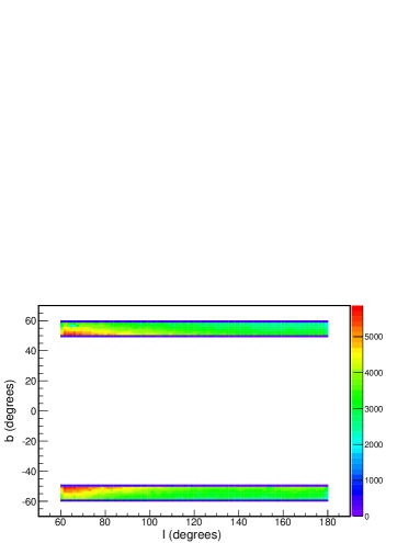
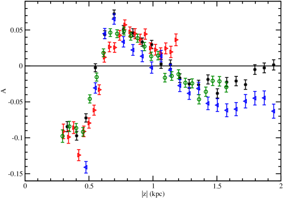
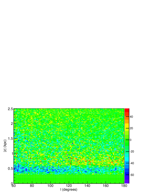
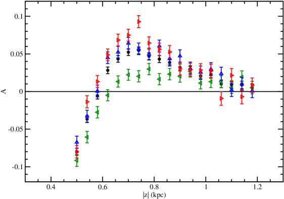
Finally we consider the Galactic longitude dependence of the asymmetry. Here we work in color, choosing the band . The analysis sample is shown in Fig. 23; it appears rather uniform, North and South. The number counts differences, North and South, are also shown in Fig. 24; here we see in the raw data a persistent excess of counts in the South, and then in the North, as we move out of the Galactic plane, for a sweep of . Finally, we report the determined North-South asymmetry in Fig. 25. In the latter we restrict our consideration to the vertical window , the range for which the sample is complete. For this larger color swatch there are some 1.98 million stars in our sample. To study the dependence, we split this sample into three forty-degree-wide bins. For , there are some 783,000 stars with a mean color of . For , there are some 635,000 stars with . For , there are some 566,000 stars with . The asymmetry for all in this color band is shown by the asterisk points in Fig. 25. We note that indeed there appears to be a significant difference in the asymmetry with , with a smaller amplitude towards the Galactic center. This is naively what one would expect for a disk which gets thicker the closer one gets to the Galactic center; it would be less responsive to a disturbing force. Our forward- and backward-looking samples, noting Fig. 2, probe regions of the disk separated by roughly 1 kpc. The longitudinal angle dependence could also be suggestive of the location of a perturbing influence. In a followup paper (Gardner et al., in preparation), we plan to examine how well-localized the asymmetry may be. We know that there are also effects due to a bar toward the Galactic center which are not completely symmetric north and south, left and right (Benjamin et al., 2005), though such effects do not figure in our present study.
5 Summary and Outlook
In the context of a larger data set we confirm and refine the earlier observation of a large North-South asymmetry in the star counts with respect to the Galactic plane (W12). We observe a peak asymmetry of some 10%, that is, roughly a peak-to-trough difference of 20%.
The strong Jeans theorem states that the matter probability distribution function in steady state can be written in terms of three isolating integrals. One of these becomes the vertical energy , which in turn goes as , having manifest even parity, as one approaches the Galactic plane (Binney & Tremaine, 2008). The appearance of our odd-parity asymmetry can be regarded as either falsifying the expected relationship as one approaches the Galactic plane, or, alternatively, as challenging the notion that the matter distribution function can written in terms of isolating integrals at all. The “ringing” nature of the asymmetry result we have found strongly favors the latter interpretation. We thus believe the asymmetry speaks to observational evidence for the failure of local gravitational equilibrium, or steady-state dynamics, in the local solar neighborhood.
We regard this as a cautionary tale for analyses which would employ equilibrium assumptions to analyze the local distribution of dark matter. While 20% density differences are well within the uncertainties of the unknown local dark matter distribution, the large velocity tail of the local dark matter phase space distribution is likely much more sensitive to such effects. We note that recent results from the RAVE velocity survey show evidence for vertical ringing in the velocity of stars at the same distances discussed here (Williams et al., 2013).
We have considered a wide range of possible systematic effects which could affect the symmetry in the distribution of stars north and south of the Galactic plane. We are able to quantify these systematics to a great extent and rule out giant/dwarf confusion, photometric parallax distance relation differences, reddening corrections, and large scale calibration errors as possible sources of the observed asymmetry. We are able to demonstrate that photometric parallax method based on SDSS photometry gives systematic and statistical distance errors of typically O(10%) at least for lower main sequence (K/M dwarf) populations. To a more limited degree, we constrain the extent to which the asymmetry can be resolved by equal-mass binary confusion, or metallicity differences, though we cannot rule out these effects completely.
Certain systematic effects are best explored through the study of distant “blue-tip” stars in our sample. By dividing the data into six bins in and exploring the properties of these stars therein, we are able to state that there are no significant localized reddening correlations beyond those of the Schlegel et al. (1998) maps. We confirm the slight color difference in noted by Schlafly et al. (2010), and we find evidence that the most likely explanation for it is a some 0.02 mag difference in the global calibration of the filter in the SDSS, as it connects the South survey region to the North survey region. We study the asymmetries in both and colors and show explicitly that the asymmetry results agree nicely without regard to which color baseline is used.
The colors of our samples are consistent with no significant color differences in the North versus the South. Regarding a possible difference in metallicity gradients, North and South, we do not have sufficient -band accuracy to perform a photometric metallicity analysis in the manner of Ivezić et al. (2008). Slight systematic differences in the average metallicity of the north versus south populations remain possible. However, no possible metallicity shift would lead to stellar density ringings confirmed here. We note that the persistence of the asymmetries observed in W12 in the current work, determined using a much larger sample of stars in a slightly different portion of the sky, also argues against the existence of idiosyncratic north-south population differences as a source of the effect.
In Gardner et al. (in preparation) we plan to analyze the symmetries associated with multiple integrals of motion simultaneously, in hope of isolating the origin of the asymmetry.
References
- Abazajian et al. (2009) Abazajian, K., Adelman-McCarthy, J.K., Agueros, M.A., et al. 2009 ApJS, 182, 543
- Aihara et al. (2011) Aihara, H., Allende Prieto, C., An, D. et al. 2011 ApJS, 193, 29
- Ahn et al. (2012) Ahn, C. P., Alexandroff, R., Allende Prieto, C. et al. 2012 ApJS, 203, 21
- An et al. (2007a) An, D., Terndrup, D. M., Pinsonneault, M. H., Paulson, D. B., Hanson, R. B., & Stauffer, J. R. 2007 ApJ, 655, 233
- An et al. (2008b) An, D., Johnson, J. A., Clem, J. L. et al., 2008 ApJS, 179, 326
- Anthony-Twarog et al. (2006) Anthony-Twarog, B. J., Tanner, D., Cracraft, M., & Twarog, B. A. 2006, AJ, 131, 461
- Benjamin et al. (2005) Benjamin, R. A., Churchwell, E., Bable, B.L. et al. 2005 ApJ 630, L149
- Berry et al. (2012) Berry, M. Ivezic, Z., Sesar, B. et al., 2012, ApJ, 757, 35
- Betoule et al. (2013) Betoule, M., Marriner, J., Regnault, N. et al. 2013 A&A 552, 124
- Binney & Tremaine (2008) Binney, J., & Tremaine, S. 2008, Galactic Dynamics: Second Edition (Princeton University Press)
- Bochanski et al. (2013) Bochanski, J.J., Savcheva, A., West, A.A. and Hawley, S.L. 2013 AJ 145, 40
- Bovy & Tremaine (2012) Bovy, J., & Tremaine, S. 2012 ApJ 756, 89
- Chen et al. (2011) Chen, Y. Q., Zhao, G., Carrell, K., Zhao, J. K., 2011, AJ, 142, 8
- Covey et al. (2007) Covey, K. R., Ivezić, Z., Schlegel, D. et al., 2007, AJ, 134, 2398
- Dame et al. (1987) Dame, T. M., Ungerechts, H., Cohen, R. S. et al. 1987, ApJ, 322, 706
- Fan et al. (1996) Fan, X., Burstein, D., Chen., J. S. et al. 1996 AJ, 112, 628
- Garbari et al. (2012) Garbari, S., Liu, C., Read, J.I., & Lake, G. 2012 MNRAS 425, 1445
- Gilmore et al. (1989) Gilmore, G., Wyse, R. F. G., & Kuijken, K 1989 ARA&A, 27, 555
- Gomez et al. (2013) Gomez, F.A., Minchev, I., O’Shea, B. W., Beers, T. C., Bullock, J. S., & Purcell, C. W. 2013 MNRAS 429, 159
- Humphreys et al. (2011) Humphreys, R. M., Beers, T.C., Cabanela, J.E., Grammer, S., Davidson, K., Lee, Y.S. & Larsen, J.A. 2011 AJ, 141, 131
- Ivezić et al. (2008) Ivezić, Ž., Sesar, B., Juric, M. et al., 2008a, ApJ, 684, 287
- Jurić et al. (2008) Jurić, M., Ivezic, Z., Brooks, A. et al. 2008 ApJ, 673, 864
- Lee et al. (2008) Lee, Y. S., Beers, T. C., Sivarani, T. et al. 2008, AJ, 136, 2050
- Majewski et al. (2003) Majewski, S. R., Skrutskie, M. F., Weinberg, M. D., Ostheimer, J. C. 2003 ApJ 599, 1082
- Marshall et al. (2006) Marshall, D. J., Robin, A. C., Reylé, C., Schultheis, M., & Picaud, S. 2006, A&A, 453, 635
- Ostriker & Peebles (1973) Ostriker, J. P. and Peebles, P. J. E. 1973, ApJ 186, 467
- Padmanabhan et al. (2008) Padmanabhan, N., Schlegel, D. J., Finkbeiner, D. P. et al. 2008 ApJ 674, 1217
- Raghavan et al. (2010) Raghavan, D., McAlister, H. A., Henry, T. J., Latham, D. W., Marcy, G. W., Mason, B. D., Gies, D. R., White, R. J., & ten Brummelaar, T. A. 2010, ApJS, 190, 1
- Schlafly et al. (2010) Schlafly, Finkbeiner, Schlegel, Jurić, Ivezić, Gibson, Knapp, & Weaver 2010, ApJ, 725, 1175
- Schlafly and Finkbeiner (2011) Schlafly, E. F., and Finkbeiner, D. P. 2011 ApJ 737, 103
- Schlesinger et al. (2012) Schlesinger, K. J., Johnson, J. A., Rockosi, C. M. et al. 2012 ApJ 761, 160
- Schlegel et al. (1998) Schlegel, D. J., Finkbeiner, D. P., & Davis, M. 1998, ApJ, 500, 525
- Widrow et al. (2012) Widrow, L. M., Gardner, S., Yanny, B., Dodelson, S., and Chen, H.Y., 2012, ApJ, 750, L41 (W12)
- Williams et al. (2013) Williams, M.E.K., Steinmetz, M., Binney, J. et al. 2013 MNRAS, in press, arXiv:1302.2468
- Yanny et al. (2009a) Yanny, B., Newberg, H. J., Johnson, J. A. et al. 2009a ApJ700, 1282
- Yanny et al. (2009b) Yanny, B., Rockosi, C., Newberg, H. J. et al., 2009b, AJ, 137, 4377
| range (in ∘) | aaThe peak color of all blue-tip (F turnoff) halo stars are tabulated North and South of the plane in three magnitude and six longitude bins, followed by the number of stars in each peak in parentheses. The Southern tip stars are significantly redder than the Northern tip stars in nearly all bins, independent of magnitude and longitude – likely indicating a large scale calibration offset. The numbers in boldface indicate the direction and distance where the Southern color is affected by Sagittarius dwarf stream stars, which are bluer than typical halo turnoff stars. N | S (peak) | N | S | N | S |
|---|---|---|---|---|---|---|
| 60 80 | 0.305 (884) | 0.316 (855) | 0.300 (673) | 0.317 (565) | 0.291(484) | 0.306(423) |
| 80 100 | 0.304 (733) | 0.320 (651) | 0.301 (552) | 0.315 (482) | 0.287(400) | 0.312(342) |
| 100 120 | 0.304 (591) | 0.333 (512) | 0.300 (465) | 0.324 (373) | 0.283(346) | 0.309(306) |
| 120 140 | 0.305 (503) | 0.320 (481) | 0.302 (400) | 0.325 (333) | 0.282(317) | 0.304(260) |
| 140 160 | 0.306 (461) | 0.299 (690) | 0.300 (367) | 0.312 (317) | 0.283(269) | 0.292(243) |
| 160 180 | 0.304 (484) | 0.299 (784) | 0.296 (382) | 0.306 (302) | 0.294(278) | 0.294(255) |