On Rényi entropies of disjoint intervals
in conformal field theory

Abstract

We study the Rényi entropies of $N$ disjoint intervals in the conformal field theories given by the free compactified boson and the Ising model. They are computed as the $2N$ point function of twist fields, by employing the partition function of the model on a particular class of Riemann surfaces. The results are written in terms of Riemann theta functions. The prediction for the free boson in the decompactification regime is checked against exact results for the harmonic chain. For the Ising model, matrix product states computations agree with the conformal field theory result once the finite size corrections have been taken into account.

Contents

toc

1 Introduction

The study of the entanglement in extended quantum systems and of its measures has attracted a lot of interest during the last decade (see the reviews [1]). Given a system in its ground state $|\Psi\rangle$, a very useful measure of entanglement is the entanglement entropy. When the Hilbert space of the full system can be factorized as $\mathcal{H}=\mathcal{H}_{A}\otimes\mathcal{H}_{B}$, the $A$’s reduced density matrix reads $\rho_{A}={\rm Tr}_{B}\rho$, being $\rho=|\Psi\rangle\langle\Psi|$ the density matrix of the entire system. The Von Neumann entropy associated to $\rho_{A}$ is the entanglement entropy

$$S_{A}=-{\rm Tr}(\rho_{A}\log\rho_{A})\,.$$ (1.1)

Introducing $S_{B}$ in an analogous way, we have $S_{B}=S_{A}$ because $\rho$ describes a pure state.

In quantum field theory the entanglement entropy (1.1) is usually computed by employing the replica trick, which consists in two steps: first one computes ${\rm Tr}\rho_{A}^{n}$ for any integer $n\geqslant 2$ (when $n=1$ the normalization condition ${\rm Tr}\rho_{A}=1$ is recovered) and then analytically continues the resulting expression to any complex $n$. This allows to obtain the entanglement entropy as $S_{A}=-\lim_{n\rightarrow 1}\partial_{n}{\rm Tr}\rho_{A}^{n}$. The Rényi entropies are defined as follows

$$S_{A}^{(n)}=\frac{1}{1-n}\,\log{\rm Tr}\rho_{A}^{n}\,.$$ (1.2)

Given the normalization condition, the replica trick tells us that $S_{A}=\lim_{n\rightarrow 1}S_{A}^{(n)}$.

In this paper we consider one dimensional critical systems when $A$ and $B$ correspond to a spatial bipartition. The simplest and most important example is the entanglement entropy of an interval $A$ of length $\ell$ in an infinite line, which is given by [2, 3, 4]

$$S_{A}=\frac{c}{3}\log\frac{\ell}{\epsilon}+c_{1}^{\prime}\,,$$ (1.3)

where $c$ is the central charge of the corresponding conformal field theory (CFT), $\epsilon$ is the UV cutoff and $c_{1}^{\prime}$ is a non universal constant. The result (1.3) has been rederived in [3] by computing ${\rm Tr}\rho_{A}^{n}$ for an interval $A=[u,v]$ as the two point function of twist fields, namely

$${\rm Tr}\rho_{A}^{n}=\frac{c_{n}}{|u-v|^{2\Delta_{n}}}\,,\qquad\Delta_{n}=\frac{c}{12}\left(n-\frac{1}{n}\right)\,,$$ (1.4)

being $\Delta_{n}$ the scaling dimension of the twist fields and $c_{n}$ a non universal constant such that $c_{1}=1$, in order to guarantee the normalization condition.

When $A$ is a single interval, ${\rm Tr}\rho_{A}^{n}$ and $S_{A}$ are sensible only to the central charge of the CFT. Instead, when the subsystem $A=\cup_{i=1}^{N}A_{i}$ consists of $N\geqslant 2$ disjoint intervals on the infinite line, the Rényi entropies encode all the data of the CFT. Denoting by $A_{i}=[u_{i},v_{i}]$ the $i$-th interval with $i=1,\dots,N$, in Fig. 1 we depict a configuration with $N=4$ disjoint intervals. By employing the method of [3, 4], ${\rm Tr}\rho_{A}^{n}$ can be computed as a $2N$ point function of twist fields. In CFT, the dependence on the positions in a $2N$ point function of primary operators with $N\geqslant 2$ is not uniquely determined by the global conformal invariance. Indeed, we have that [4]

$${\rm Tr}\rho_{A}^{n}=c_{n}^{N}\left|\,\frac{\prod_{i<j}(u_{j}-u_{i})(v_{j}-v_{i})}{\prod_{i,j}(v_{j}-u_{i})}\,\right|^{2\Delta_{n}}\mathcal{F}_{N,n}(\boldsymbol{x})\,,$$ (1.5)

where $\mathcal{F}_{N,n}(\boldsymbol{x})$ is a model dependent function of the $2N-3$ independent variables $0<x_{1}<\dots<x_{2N-3}<1$ (indicated by the vector $\boldsymbol{x}$), which are the invariant ratios that can be built with the $2N$ endpoints of the intervals through a conformal map.

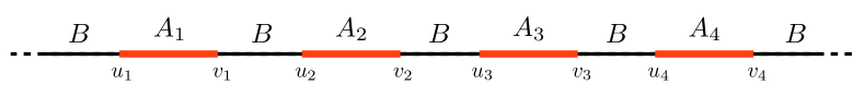
Figure 1: A typical configuration of disjoint intervals in the infinite line. We consider the entanglement between $A=\cup_{i=1}^{N}A_{i}$ (in this figure $N=4$) and its complement $B$.

For $N=2$ intervals there is only one harmonic ratio $0<x<1$. The function $\mathcal{F}_{2,n}(x)$ has been computed for the free boson compactified on a circle [5] and for the Ising model [6]. A crucial role in the derivation is played by the methods developed in [7, 8, 9, 10, 11, 12, 13, 14] to study CFT on higher genus Riemann surfaces. The results are expressed in terms of Riemann theta functions [15, 16, 17] and it is still an open problem to compute their analytic continuation in $n$ for the most general case, in order to get the entanglement entropy $S_{A}$. These CFT predictions are supported by numerical studies performed through various methods [18, 19, 20, 21, 22, 23, 24, 25].

For three or more intervals, few analytic results are available in the literature. For instance, the Rényi entropies of $N>2$ disjoint intervals for the Dirac fermion in two dimensions has been computed in [26, 27, 28]. This result holds for a specific sector and it is not modular invariant [29].

In this paper we compute $\mathcal{F}_{N,n}(\boldsymbol{x})$ with $N\geqslant 2$ for the free boson compactified on a circle and for the Ising model, by employing the results of [7, 9, 10, 11, 14] and [30]. The case $n=2$ has been studied in [7] and its extension to $n>2$ has been already discussed in [12, 13, 5, 29]. Here we provide explicit expressions for $\mathcal{F}_{N,n}(\boldsymbol{x})$ in terms of Riemann theta functions. The free boson on the infinite line is obtained as a limiting regime and the corresponding CFT predictions have been checked against exact numerical results for the harmonic chain. The numerical checks of the CFT formulas for the Ising model have been done by employing the Matrix Product States (MPS) [31, 32].

We remark that, in the case of several disjoint intervals, the entanglement entropy $S_{A}$ measures the entanglement of the union of the intervals with the rest of the system $B$. It is not a measure of the entanglement among the intervals, whose union is in a mixed state. In order to address this issue, one needs to consider other quantities which measure the entanglement for mixed states. An interesting example is the negativity [33, 34], which has been studied for a two dimensional CFT in [35, 36] by employing the twist fields method (see [37, 38, 39] for the Ising model).

In the context of the AdS/CFT correspondence, there is a well estabilished prescription to compute $S_{A}$ in generic spacetime dimensions through the gravitational background in the bulk [40, 41, 42], which has been applied also in the case of disjoint regions [43, 44, 45, 46, 47]. Proposals for the holographic computation of the Rényi entropies $S_{A}^{(n)}$ are also available [48, 49, 50, 51, 52]. The holographic methods hold in the regime of large $c$, while the models that we consider here have $c=1$ and $c=1/2$.

The layuot of the paper is as follows. In §2 we describe the relation between ${\rm Tr}\rho_{A}^{n}$ and the partition functions of two dimensional conformal field theories on the particular class of Riemann surfaces occurring in our problem. In §3 we compute the Rényi entropies for the free compactified boson in the generic case of $N$ intervals and $n$ sheets, which allows us to write the same quantity also for the Ising model. In §4 we discuss how the known case of two intervals is recovered. In §5 we check the CFT predictions for the free boson in the decompactification regime against exact results obtained for the harmonic chain with periodic boundary conditions. In §6 numerical results obtained with MPS for the Ising model with periodic boundary conditions are employed to check the corresponding CFT prediction through a finite size scaling analysis. In the Appendices, we collect further details and results.

2 Rényi entropies and Riemann surfaces

Given a two dimensional quantum field theory, let us consider a spatial subsystem $A=\cup_{i=1}^{N}A_{i}$ made by $N$ disjoint intervals $A_{1}=[u_{1},v_{1}]$, $\dots$, $A_{N}=[u_{N},v_{N}]$.

The path integral representation of $\rho_{A}$ has been largely discussed in [2, 3, 4]. Tracing over the spatial complement $B$ leaves open cuts, one for each interval, along the line characterized by a fixed value of the Euclidean time. Thus, the path integral giving $\rho_{A}$ involves fields which live on this sheet with open cuts, whose configurations are fixed on the upper and lower parts of the cuts.

To compute ${\rm Tr}\rho_{A}^{n}$, we take $n$ copies of the path integral representing $\rho_{A}$ and combine them as briefly explained in the following. For any fixed $x\in A$, we impose that the value of a field on the upper part of the cut on a sheet is equal to the value of the same field on the lower part of the corresponding cut on the sheet right above. This condition is applied in a cyclic way. Then, we integrate over the field configurations along the cuts. Correspondingly, the $n$ sheets must be sewed in the same way and this procedure defines the $n$-sheeted Riemann surface $\mathscr{R}_{N,n}$. The endpoints $u_{i}$ and $v_{i}$ ($i=1,\dots,N$) are branch points where the $n$ sheets meet. The Riemann surface $\mathscr{R}_{N,n}$ is depicted in Fig. 2 for $N=3$ intervals and $n=3$ copies. Denoting by $\mathcal{Z}_{N,n}$ the partition function of the model on the Riemann surface $\mathscr{R}_{N,n}$, we can compute ${\rm Tr}\rho_{A}^{n}$ as [3]

$${\rm Tr}\rho_{A}^{n}=\frac{\mathcal{Z}_{N,n}}{\mathcal{Z}^{n}}\,,$$ (2.1)

where $\mathcal{Z}=\mathcal{Z}_{0,1}$ is the partition function of the model defined on a single copy and without cuts. Notice that (2.1) implies ${\rm Tr}\rho_{A}=1$. From (2.1), one easily gets the Rényi entropies (1.2). If the analytic continuation of (2.1) to $\textrm{Re}\,n>1$ exists and it is unique, the entanglement entropy is obtained as the replica limit

$$S_{A}=\lim_{n\,\rightarrow\,1}S_{A}^{(n)}=\,-\lim_{n\,\rightarrow\,1}\frac{\partial}{\partial n}\,{\rm Tr}\rho_{A}^{n}\,.$$ (2.2)

In order to find the genus of $\mathscr{R}_{N,n}$ [8], let us consider a single sheet and triangulate it through $V$ vertices, $E$ edges and $F$ faces, such that $2N$ vertices are located at the branch points $u_{i}$ and $v_{i}$. Considering $\mathscr{R}_{N,n}$ constructed as explained above, the replication of the same triangulation on the other sheets generates a triangulation of the Riemann surface $\mathscr{R}_{N,n}$ made by $V^{\prime}$ vertices, $E^{\prime}$ edges and $F^{\prime}$ faces. Notice that, since the branch points belong to all the $n$ sheets, they are not replicated. This observation tells us that $V^{\prime}=n(V-2N)+2N$, while $E^{\prime}=nE$ and $F^{\prime}=nF$ because all the edges and the faces are replicated. Then, the genus $g$ of $\mathscr{R}_{N,n}$ is found by plugging these expressions into the relation $V^{\prime}-E^{\prime}+F^{\prime}=2-2g$ and employing the fact that, since each sheet has the topology of the sphere, $V-E+F=2$. The result is

$$g=(N-1)(n-1)\,.$$ (2.3)

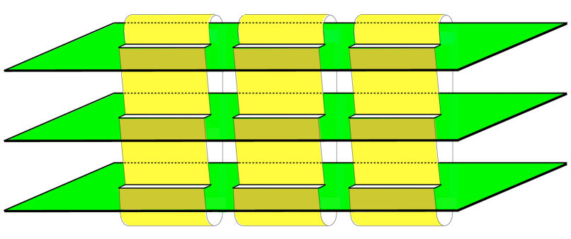
Figure 2: The path integral representation of $\textrm{Tr}\rho_{A}^{n}$ involves a Riemann surface $\mathscr{R}_{N,n}$, which is shown here for $N=3$ and $n=3$.

We remark that we are not considering the most general genus $g$ Riemann surface, which is characterized by $3g-3$ complex parameters, but only the subclass of Riemann surfaces obtained through the replication procedure.

Let us consider a conformal field theory with central charge $c$. As widely argued in [3, 4], in the case of one interval $A=[u,v]$ in an infinite line, ${\rm Tr}\rho_{A}^{n}$ can be written as the two point function of twist fields on the complex plane plus the point at infinity, i.e.

$${\rm Tr}\rho_{A}^{n}=\langle\mathcal{T}_{n}(u)\bar{\mathcal{T}}_{n}(v)\rangle=\frac{c_{n}}{|u-v|^{2\Delta_{n}}}\,,\qquad\Delta_{n}=\frac{c}{12}\left(n-\frac{1}{n}\right).$$ (2.4)

Both the twist field $\mathcal{T}_{n}$ and $\bar{\mathcal{T}}_{n}$, also called branch point twist fields [53], have the same scaling dimension $\Delta_{n}$. The constant $c_{n}$ is non universal and such that $c_{1}=1$ because of the normalization condition.

Similarly, when $A$ consists of $N\geqslant 2$ disjoint intervals $A_{i}=[u_{i},v_{i}]$ with $i=1,\dots,N$, ordered on the infinite line according to $i$, namely $u_{1}<v_{1}<\dots<u_{N}<v_{N}$, we can write ${\rm Tr}\rho_{A}^{n}$ as the following $2N$ point function of twist fields

$${\rm Tr}\rho_{A}^{n}=\langle\prod_{i\,=1}^{N}\mathcal{T}_{n}(u_{i})\bar{\mathcal{T}}_{n}(v_{i})\rangle\,.$$ (2.5)

In the case of four and higher point correlation functions of primary fields, the global conformal invariance does not fix the precise dependence on $u_{i}$ and $v_{i}$ because one can construct invariant ratios involving these points. In particular, let us consider the conformal map such that $u_{1}\rightarrow 0$, $u_{N}\rightarrow 1$ and $v_{N}\rightarrow\infty$, namely

$$w_{N}(z)=\frac{(u_{1}-z)(u_{N}-v_{N})}{(u_{1}-u_{N})(z-v_{N})}\,.$$ (2.6)

The remaining $u_{i}$’s and $v_{j}$’s are sent into the $2N-3$ harmonic ratios $x_{1}=w_{N}(v_{1})$, $x_{2}=w_{N}(u_{2})$, $x_{3}=w_{N}(v_{2})$, $\dots$, $x_{2N-3}=w_{N}(v_{N-1})$ which are invariant under $SL(2,\mathbb{C})$ transformations. The map (2.6) preserves the ordering: $0<x_{1}<x_{2}<\dots<x_{2N-3}<1$. We denote by $\boldsymbol{x}$ the vector whose elements are the harmonic ratios $x_{1},\dots,x_{2N-3}$.
Global conformal invariance allows to write the $2N$ point function (2.5) as [4]

$${\rm Tr}\rho_{A}^{n}=c_{n}^{N}\left|\,\frac{\prod_{i<j}(u_{j}-u_{i})(v_{j}-v_{i})}{\prod_{i,j}(v_{j}-u_{i})}\,\right|^{2\Delta_{n}}\mathcal{F}_{N,n}(\boldsymbol{x})\,,$$ (2.7)

where $i,j=1,\dots,N$. The function $\mathcal{F}_{N,n}(\boldsymbol{x})$ encodes the full operator content of the model and therefore it must be computed through its dynamical details. Since ${\rm Tr}\rho_{A}=1$, we have $\mathcal{F}_{N,1}(\boldsymbol{x})=1$. In the case of two intervals, $\mathcal{F}_{2,n}(\boldsymbol{x})$ has been computed for the free compactified boson [5] and for the Ising model [6]. We remark that the domain of $\mathcal{F}_{N,n}(\boldsymbol{x})$ is $0<x_{1}<\dots<x_{2N-3}<1$ (see Fig. 3 for $N=3$).

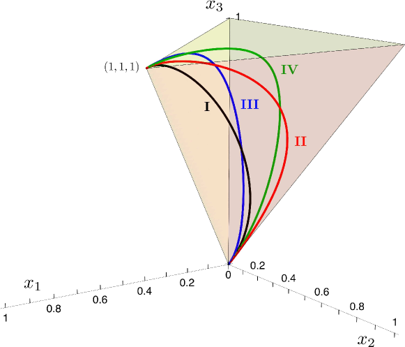
Figure 3: The domain $0<x_{1}<x_{2}<x_{3}<1$ of the function $\mathcal{F}_{3,n}(\boldsymbol{x})$. The lines within this domain are the configurations defined in (5.14).

The expression (2.7) is UV divergent. Such divergence is introduced dividing any length occurring in the formula ($u_{j}-u_{i}$, $v_{j}-u_{i}$, etc.) by the UV cutoff $\epsilon$. Since the ratios $\boldsymbol{x}$ are left unchanged, the whole dependence on $\epsilon$ of (2.7) comes from the ratio of lengths within the absolute value, which gives $\epsilon^{2N\Delta_{n}}$.

It is useful to introduce some quantities which are independent of the UV cutoff. For $N=2$, we can construct a combination of Rényi entropies having this property as follows

$$I^{(n)}_{A_{1},A_{2}}\equiv S^{(n)}_{A_{1}}+S^{(n)}_{A_{2}}-S^{(n)}_{A_{1}\cup A_{2}}=\frac{1}{n-1}\,\log\bigg{(}\frac{{\rm Tr}\rho^{n}_{A_{1}\cup A_{2}}}{{\rm Tr}\rho^{n}_{A_{1}}{\rm Tr}\rho^{n}_{A_{2}}}\bigg{)}.$$ (2.8)

The limit $n\rightarrow 1$ of this quantity defines the mutual information $I_{A_{1},A_{2}}$

$$I_{A_{1},A_{2}}\equiv S_{A_{1}}+S_{A_{2}}-S_{A_{1}\cup A_{2}}=\lim_{n\,\rightarrow\,1}I^{(n)}_{A_{1},A_{2}}\,,$$ (2.9)

which is independent of the UV cutoff as well. The subadditivity of the entanglement entropy tells us that $I_{A_{1},A_{2}}\geqslant 0$, while the strong subadditivity implies that it increases when one of the intervals is enlarged.

For $N>2$ we can find easily two ways to construct quantities such that the short distance divergence cancels. Let us consider first the following ratio

$$R_{N,n}\equiv\prod_{p\,=\,1}^{N}\;\prod_{\sigma_{N,p}}\big{(}{\rm Tr}\rho^{n}_{\sigma_{N,p}}\big{)}^{(-1)^{N-p}},$$ (2.10)

where we denoted by $\sigma_{N,p}$ a generic choice of $1\leqslant p\leqslant N$ intervals among the $N$ ones we are dealing with. Since ${\rm Tr}\rho^{n}_{\sigma_{N,p}}$ goes like $\epsilon^{2p\Delta_{n}}$, one finds that (2.10) is independent of $\epsilon$ by employing that $\sum_{p=1}^{N}(-1)^{N-p}\binom{N}{p}p=0$. In the simplest cases of $N=2$ and $N=3$, the ratio (2.10) reads

$$R_{2,n}=\frac{{\rm Tr}\rho^{n}_{\{1,2\}}}{{\rm Tr}\rho^{n}_{\{1\}}\,{\rm Tr}\rho^{n}_{\{2\}}}\,,\qquad R_{3,n}=\frac{{\rm Tr}\rho^{n}_{\{1,2,3\}}\,\big{(}{\rm Tr}\rho^{n}_{\{1\}}\,{\rm Tr}\rho^{n}_{\{2\}}\,{\rm Tr}\rho^{n}_{\{3\}}\big{)}}{{\rm Tr}\rho^{n}_{\{1,2\}}\,{\rm Tr}\rho^{n}_{\{1,3\}}\,{\rm Tr}\rho^{n}_{\{2,3\}}}\,,\qquad\dots$$ (2.11)

In order to generalize (2.8) for $N\geqslant 2$, one introduces

$$I_{A_{1},\dots,A_{N}}^{(n)}\equiv\frac{(-1)^{N}}{n-1}\log R_{N,n}\,,$$ (2.12)

and its limit $n\rightarrow 1$, as done in (2.9) for $N=2$, i.e.

$$I_{A_{1},\dots,A_{N}}\equiv\lim_{n\rightarrow 1}I_{A_{1},\dots,A_{N}}^{(n)}\,.$$ (2.13)

For the simplest cases of $N=3$ and $N=4$, one finds respectively

$$I_{A_{1},A_{2},A_{3}} = S_{A_{1}}+S_{A_{2}}+S_{A_{3}}-S_{A_{1}\cup A_{2}}-S_{A_{1}\cup A_{3}}-S_{A_{2}\cup A_{3}}+S_{A_{1}\cup A_{2}\cup A_{3}}\,,$$ (2.14)

$$\rule{0.0pt}{22.76228pt}I_{A_{1},A_{2},A_{3},A_{4}} = \sum_{i=1}^{4}S_{A_{i}}-\sum_{\begin{subarray}{c}i,j=1\\ i\,<\,j\end{subarray}}^{4}S_{A_{i}\cup A_{j}}+\sum_{\begin{subarray}{c}i,j,k=1\\ i<j<k\end{subarray}}^{4}S_{A_{i}\cup A_{j}\cup A_{k}}-S_{A_{1}\cup A_{2}\cup A_{3}\cup A_{4}}\,.$$ (2.15)

The quantity $I_{A_{1},A_{2},A_{3}}$ is called tripartite information [27] and it provides a way to establish whether the mutual information is extensive ($I_{A_{1},A_{2},A_{3}}=0$) or not. In a general quantum field theory there is no definite sign for $I_{A_{1},A_{2},A_{3}}$, but for theories with a holographic dual it has been shown that $I_{A_{1},A_{2},A_{3}}\leqslant 0$ [47].

Another cutoff independent ratio is given by

$$\tilde{R}_{N,n}\equiv\frac{{\rm Tr}\rho_{A}^{n}}{\prod_{i=1}^{N}{\rm Tr}\rho_{A_{i}}^{n}}\,.$$ (2.16)

When $N=2$ we have $R_{2,n}=\tilde{R}_{2,n}$ but (2.10) and (2.16) are different for $N>2$.
From the definitions (2.10) and (2.16), we observe that, when one of the intervals collapses to the empty set, i.e. $A_{k}\rightarrow\emptyset$ for some $k\in\{1,\dots,N\}$, we have that $R_{N,n}\rightarrow 1$ and $\tilde{R}_{N,n}\rightarrow\tilde{R}_{N-1,n}$, where $\tilde{R}_{N-1,n}$ is defined through $A\setminus A_{k}$.

For two dimensional conformal field theories at zero temperature we can write $R_{N,n}$ and $\tilde{R}_{N,n}$ more explicitly. In particular, plugging (2.4) and (2.7) into (2.16), it is straightforward to observe that $c_{n}$ simplifies and we are left with

$$\tilde{R}_{N,n}(\boldsymbol{x})=\bigg{|}\prod_{i<j}\frac{(u_{i}-u_{j})(v_{i}-v_{j})}{(u_{i}-v_{j})(u_{j}-v_{i})}\,\bigg{|}^{2\Delta_{n}}\mathcal{F}_{N,n}(\boldsymbol{x})\equiv|p_{N}(\boldsymbol{x})|^{2\Delta_{n}}\,\mathcal{F}_{N,n}(\boldsymbol{x})\,,$$ (2.17)

where the product within the absolute value, that we denote by $p_{N}$, can be written in terms of $\boldsymbol{x}$. Thus, (2.17) tells us that $\mathcal{F}_{N,n}(\boldsymbol{x})$ can be easily obtained from $\tilde{R}_{N,n}(\boldsymbol{x})$. When $N=2$ we have $p_{2}(x)=-1/(1-x)$, while for $N=3$ we find

$$p_{3}(\boldsymbol{x})\equiv-\frac{(x_{3}-x_{1})(1-x_{2})\,x_{2}}{(x_{2}-x_{1})(1-x_{1})(1-x_{3})\,x_{3}}\,.$$ (2.18)

For higher values of $N$, the expression of $p_{N}(\boldsymbol{x})$ is more complicated.

As for $R_{N,n}$ in (2.10), considering the choice of intervals given by $\sigma_{N,p}$, we have

$${\rm Tr}\rho_{\sigma_{N,p}}^{n}=c_{n}^{p}\,\big{|}P_{p}(\sigma_{N,p})\big{|}^{2\Delta_{n}}\,\mathcal{F}_{p,n}(\boldsymbol{x}^{\sigma_{N,p}})\,,$$ (2.19)

where

$$P_{p}(\sigma_{N,p})\equiv\left.\frac{\prod_{i<j}(u_{j}-u_{i})(v_{j}-v_{i})}{\prod_{i,j}(v_{j}-u_{i})}\,\right|_{\,i,j\,\in\,\sigma_{N,p}}\,,$$ (2.20)

and $\boldsymbol{x}^{\sigma_{N,p}}$ denotes the $2p-3$ harmonic ratios that can be constructed through the $2p$ endpoints of the intervals of $A$ specified by $\sigma_{N,p}$. Notice that (2.19) becomes (2.7) when $p=N$ and (2.4) for $p=1$ because $\mathcal{F}_{N,1}=1$ by definition and $P_{1}(\sigma_{N,1})=1/(v_{j}-u_{j})$, being $j$ the interval specified by $\sigma_{N,1}$. Moreover, since (2.20) can be written in terms of the $2N-3$ elements of $\boldsymbol{x}$, we have that $R_{N,n}=R_{N,n}(\boldsymbol{x})$ (see Appendix A for more details). Plugging (2.19) into (2.10), one finds that for $N>2$ all the factors $P_{p}(\sigma_{N,p})$ cancel (this simplification is explained in Appendix A) and therefore we have

$$R_{N,n}(\boldsymbol{x})=\prod_{p\,=\,2}^{N}\,\prod_{\sigma_{N,p}}\big{[}\mathcal{F}_{p,n}(\boldsymbol{x}^{\sigma_{N,p}})\big{]}^{(-1)^{N-p}}.$$ (2.21)

In order to cancel those parameters which occur only through multiplicative factors, we find it useful to normalize the quantities we introduced by themselves computed for a fixed configuration. Thus, for (2.10) and (2.13) we have respectively

$$R^{\textrm{\tiny{norm}}}_{N,n}\equiv\frac{R_{N,n}}{R_{N,n}\big{|}_{\textrm{\tiny{fixed configuration}}}}\,,\qquad I^{\textrm{\tiny{sub}}}_{N}\equiv I_{N}-I_{N}\big{|}_{\textrm{\tiny{fixed configuration}}}\,,$$ (2.22)

where we adopted the shorthand notation $I_{N}\equiv I_{A_{1},\dots,A_{N}}$. In conformal field theories, for the scale invariant quantities depending on the harmonic ratios $\boldsymbol{x}$, the fixed configuration is characterized by fixed values $\boldsymbol{x}_{\textrm{\tiny{fixed}}}$. For instance, we have

$$R^{\textrm{\tiny{norm}}}_{N,n}(\boldsymbol{x})=\frac{R_{N,n}(\boldsymbol{x})}{R_{N,n}(\boldsymbol{x}_{\textrm{\tiny{fixed}}})}\,,\qquad\mathcal{F}^{\textrm{\tiny{norm}}}_{N,n}(\boldsymbol{x})=\frac{\mathcal{F}_{N,n}(\boldsymbol{x})}{\mathcal{F}_{N,n}(\boldsymbol{x}_{\textrm{\tiny{fixed}}})}\,.$$ (2.23)

In §5 this normalization is adopted to study the free boson on the infinite line.

3 Free compactified boson

In this section we consider the real free boson $\phi(z,\bar{z})$ on the Riemann surface $\mathscr{R}_{N,n}$ and compactified on a circle of radius $R$. Its action reads

$$S[\phi]\propto\int_{\mathscr{R}_{N,n}}\partial_{z}\phi\,\partial_{\bar{z}}\phi\,d^{2}z\,.$$ (3.1)

The worldsheet is $\mathscr{R}_{N,n}$ and the target space is $\mathbb{R}/(2\pi R\,\mathbb{Z})$. This model has $c=1$ and its partition function for a generic compact Riemann surface of genus $g$ has been largely discussed in the literature (see e.g. [7, 9, 10, 14, 12, 13]).

Instead of working with a single field $\phi$ on $\mathscr{R}_{N,n}$, one could equivalently consider $n$ independent copies of the model with a field $\phi_{j}$ on the $j$-th sheet [26, 53]. These $n$ fields are coupled through their boundary conditions along the cuts $A_{i}$ on the real axis in a cyclic way (see Fig. 4)

$$\phi_{j}(x,0^{+})=\phi_{j+1}(x,0^{-})\,,\qquad x\in A\,,\qquad j\in\{1,\dots,n\}\,,\qquad n+1\equiv 1\,.$$ (3.2)

This approach has been adopted in [5] for the $N=2$ case, employing the results of [8]. In principle one should properly generalize the construction of [5] to $N>2$. For $n=2$ this computation has been done in [7]. Here, instead, in order to address the case $n>2$, we compute (2.7) for the model (3.1) more directly, borrowing heavily from the literature about the free compactified boson on higher genus Riemann surfaces, whose partition function has been constructed in terms of the period matrix of the underlying Riemann surface.

3.1 The period matrix

The $n$-sheeted Riemann surface $\mathcal{R}_{N,n}$ obtained by considering $N$ intervals $A_{i}=[u_{i},v_{i}]$ ($i=1,\dots,N$) is defined by the following complex curve in $\mathbb{C}^{2}$ [30]

$$y^{n}=u(z)v(z)^{n-1}\,,\qquad u(z)=\prod_{\gamma\,=\,1}^{N}(z-x_{2\gamma-2})\,,\qquad v(z)=\prod_{\gamma\,=\,1}^{N-1}(z-x_{2\gamma-1})\,.$$ (3.3)

The complex coordinates $y$ and $z$ parameterize $\mathbb{C}^{2}$ and in $u(z)$ we introduced $x_{0}\equiv 0$ and $x_{2N-2}\equiv 1$ for notational convenience. For $n=2$, the curve (3.3) is hyperelliptic. The genus of $\mathcal{R}_{N,n}$ is (2.3) and it can be found also by applying the Riemann-Hurwitz formula for the curve (3.3).

The period matrix of the curve (3.3) has been computed in [30] by considering the following non normalized basis of holomorphic differentials

$$\omega_{\alpha,j}=\frac{z^{\alpha-1}\,v(z)^{j-1}}{y^{j}}\,dz\,,\qquad\alpha=1,\dots,N-1\,,\qquad j=1,\dots,n-1\,,$$ (3.4)

where $y=y(z)$ through (3.3). The set of one forms defined in (3.4) contains $g$ elements.
In (3.4) we employed a double index notation: a greek index for the intervals and a latin one for the sheets. We make this choice to facilitate the comparison with [5], slightly changing the notation with respect to the previous section. These two indices can be combined either as $r=\alpha+(N-1)(j-1)$ [30] or $r=j+(n-1)(\alpha-1)$ [29] in order to have an index $r=1,\dots,g$. Hereafter we assume the first choice. Notice that for the cases of $(N,n)=(2,n)$ and $(N,n)=(N,2)$ we do not need to introduce this distinction.

The period matrix of the Riemann surface is defined in terms of a canonical homology basis, namely a set of $2g$ closed oriented curves $\{a_{r},b_{r}\}$ which cannot be contracted to a point and whose intersections satisfy certain simple relations. In particular, defining the intersection number $h\circ\tilde{h}$ between two oriented curves $h$ and $\tilde{h}$ on the Riemann surface as the number of intersection points, with the orientation taken into account (through the tangent vectors at the intersection point and the right hand rule), for a canonical homology basis we have $a_{r}\circ a_{s}=b_{r}\circ b_{s}=0$ and $a_{r}\circ b_{s}=-\,b_{r}\circ a_{s}=\delta_{rs}$. By employing the double index notation mentioned above, we choose the canonical homology basis $\{a_{\alpha,j},b_{\alpha,j}\}$ adopted in [30], which is depicted in Fig. 4 and in Fig. 5 for the special case of $N=3$ intervals and $n=4$ sheets.

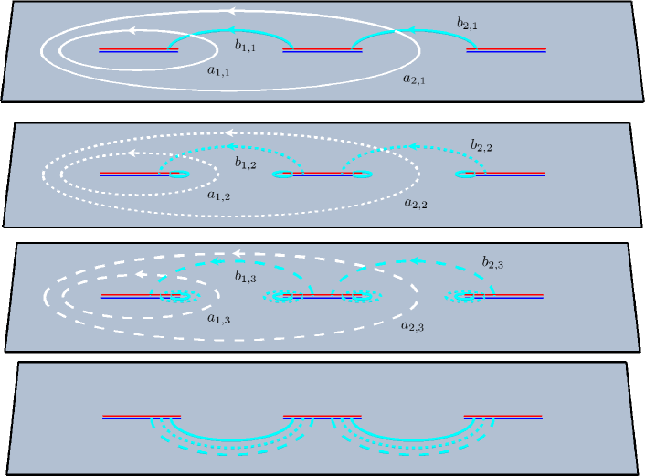
Figure 4: The canonical homology basis $\{a_{\alpha,j},b_{\alpha,j}\}$ for $N=3$ intervals of equal length and $n=4$ sheets. The sheets are ordered starting from the top. For each cut, the upper part (red) is identified with the lower part (blue) of the corresponding cut on the next sheet in a cyclic way, according to (3.2).

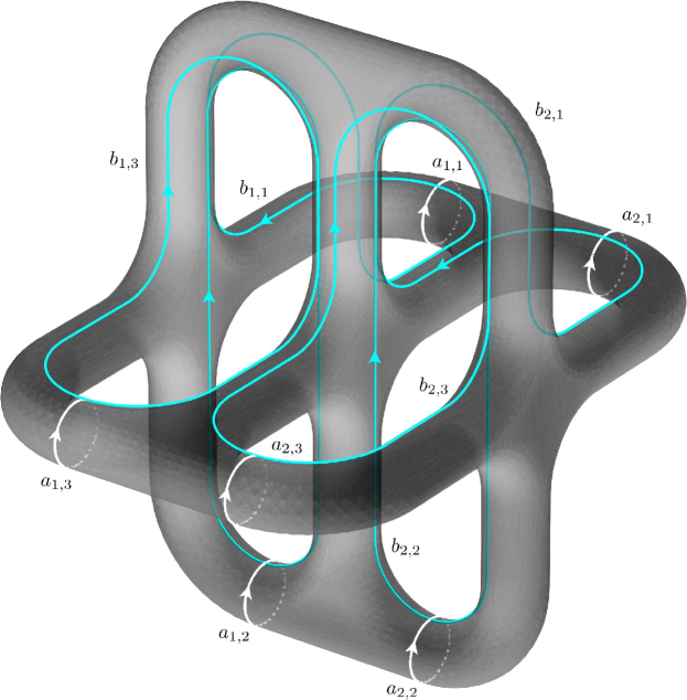
Figure 5: The Riemann surface $\mathscr{R}_{3,4}$ with the canonical homology basis $\{a_{\alpha,j},b_{\alpha,j}\}$, represented also in Fig. 4.

Once the canonical homology basis has been chosen, we introduce the $g\times g$ matrices

$$\mathcal{A}_{k,j}^{\beta,\alpha}=\oint_{a_{\alpha,j}}\omega_{\beta,k}\,,\qquad\mathcal{B}_{k,j}^{\beta,\alpha}=\oint_{b_{\alpha,j}}\omega_{\beta,k}\,,$$ (3.5)

where latin and greek indices run as in (3.4). Given the convention adopted above, $\mathcal{A}_{k,j}^{\beta,\alpha}$ provides the element $\mathcal{A}_{rs}$ of the $g\times g$ matrix $\mathcal{A}$ by setting $r=\beta+(N-1)(k-1)$ and $s=\alpha+(N-1)(j-1)$ (similarly for $\mathcal{B}$), namely the row index is determined by the one form and the column index by the cycle. This connection among indices is important because the matrices $\mathcal{A}$ and $\mathcal{B}$ are not symmetric.

From the one forms (3.4) and the matrix $\mathcal{A}$ in (3.5), one constructs the normalized basis of one forms $\nu_{r}=\sum_{s=1}^{g}\mathcal{A}^{-1}_{rs}\omega_{s}$, which provides the period matrix $\tau$ as follows

$$\oint_{a_{r}}\nu_{s}=\delta_{rs}\,,\qquad\oint_{b_{r}}\nu_{s}=\tau_{rs}\,,\qquad r,s=1,\dots,g\,.$$ (3.6)

The period matrix $\tau$ is a $g\times g$ complex and symmetric matrix with positive definite imaginary part, i.e. it belongs to the Siegel upper half space. Substituting the expression of $\nu_{s}$ into the definition of $\tau$ in (3.6) and employing the definition of the matrix $\mathcal{B}$ in (3.5), it is straightforward to observe that

$$\tau\,=\,\mathcal{A}^{-1}\cdot\mathcal{B}\,\equiv\,\mathcal{R}+{\rm i}\,\mathcal{I}\,,$$ (3.7)

where $\mathcal{R}$ and $\mathcal{I}$ are respectively the real and the imaginary part of the period matrix.

In order to compute the period matrix (3.7), let us introduce the set of auxiliary cycles $\{a^{\textrm{\tiny aux}}_{\alpha,j},b^{\textrm{\tiny aux}}_{\alpha,j}\}$, which is represented in Figs. 27 and 28. It is clear that this set is not a canonical homology basis. Indeed, some cycles intersect more than one cycle. Nevertheless, we can use them to decompose the cycles of the basis $\{a_{\alpha,j},b_{\alpha,j}\}$ as

$$a_{\alpha,j}=\sum_{\gamma\,=\,1}^{\alpha}a^{\textrm{\tiny aux}}_{\gamma,j}\,,\qquad b_{\alpha,j}=\sum_{l\,=\,j}^{n-1}b^{\textrm{\tiny aux}}_{\alpha,l}\,.$$ (3.8)

Integrating the one forms (3.4) along the auxiliary cycles as shown in (3.5) for the basis $\{a_{\alpha,j},b_{\alpha,j}\}$, one defines the matrices $\mathcal{A}^{\textrm{\tiny aux}}$ and $\mathcal{B}^{\textrm{\tiny aux}}$. The advantage of the auxiliary cycles is that the integrals $(\mathcal{A}^{\textrm{\tiny aux}})^{\beta,\alpha}_{k,j}$ and $(\mathcal{B}^{\textrm{\tiny aux}})^{\beta,\alpha}_{k,j}$ on the $j$-th sheet are obtained multiplying the corresponding ones on the first sheet by a phase [8]

$$(\mathcal{A}^{\textrm{\tiny aux}})^{\beta,\alpha}_{k,j}=\rho_{n}^{k(j-1)}(\mathcal{A}^{\textrm{\tiny aux}})^{\beta,\alpha}_{k,1}\,,\qquad(\mathcal{B}^{\textrm{\tiny aux}})^{\beta,\alpha}_{k,j}=\rho_{n}^{k(j-1)}(\mathcal{B}^{\textrm{\tiny aux}})^{\beta,\alpha}_{k,1}\,,\qquad\rho_{n}\equiv e^{2\pi\textrm{i}/n}\,.$$ (3.9)

Because of the relation (3.8) among the cycles of the canonical homology basis and the auxiliary ones, the matrices $\mathcal{A}$ and $\mathcal{B}$ in (3.5) are related to $\mathcal{A}^{\textrm{\tiny aux}}$ and $\mathcal{B}^{\textrm{\tiny aux}}$ as

$$\mathcal{A}^{\beta,\alpha}_{k,j}=\sum_{\gamma\,=\,1}^{\alpha}(\mathcal{A}^{\textrm{\tiny aux}})^{\beta,\gamma}_{k,j}=\rho_{n}^{k(j-1)}\sum_{\gamma\,=\,1}^{\alpha}(\mathcal{A}^{\textrm{\tiny aux}})^{\beta,\gamma}_{k,1}\,,$$ (3.10)

$$\mathcal{B}^{\beta,\alpha}_{k,j}=\sum_{l\,=\,j}^{n-1}(\mathcal{B}^{\textrm{\tiny aux}})^{\beta,\alpha}_{k,l}=\sum_{l\,=\,j}^{n-1}\rho_{n}^{k(l-1)}(\mathcal{B}^{\textrm{\tiny aux}})^{\beta,\alpha}_{k,1}=\frac{\rho_{n}^{kj}-1}{\rho_{n}^{k}(1-\rho_{n}^{k})}\,(\mathcal{B}^{\textrm{\tiny aux}})^{\beta,\alpha}_{k,1}\,,$$ (3.11)

where the relations (3.9) have been used. Thus, from (3.10) and (3.11) we learn that we just need $(\mathcal{A}^{\textrm{\tiny aux}})^{\beta,\alpha}_{k,1}$ and $(\mathcal{B}^{\textrm{\tiny aux}})^{\beta,\alpha}_{k,1}$ to construct the matrices $\mathcal{A}$ and $\mathcal{B}$.

By carefully considering the phases in the integrand along the cycles, we find

$$(\mathcal{A}^{\textrm{\tiny aux}})^{\beta,\alpha}_{k,1}=\oint_{a^{\textrm{\tiny aux}}_{\alpha,1}}\omega_{\beta,k} = (-1)^{N-\alpha}(\rho_{n}^{-k}-1)\,\mathscr{I}_{\beta,k}\big{|}_{x_{2\alpha-2}}^{x_{2\alpha-1}}\,,$$ (3.12)

$$\rule{0.0pt}{19.91684pt}(\mathcal{B}^{\textrm{\tiny aux}})^{\beta,\alpha}_{k,1}=\oint_{b^{\textrm{\tiny aux}}_{\alpha,1}}\omega_{\beta,k} = (-1)^{N-\alpha}\rho_{n}^{k/2}(\rho_{n}^{-k}-1)\,\mathscr{I}_{\beta,k}\big{|}_{x_{2\alpha-1}}^{x_{2\alpha}}\,,$$ (3.13)

where we introduced the following integral

$$\mathscr{I}_{\beta,k}\big{|}_{a}^{b}\equiv\int_{0}^{1}\frac{(b-a)\,\big{[}(b-a)t+a\big{]}^{\beta-1-k/n}\;dt}{\prod_{\gamma=2}^{N}\big{|}(b-a)t-(x_{2\gamma-2}-a)\big{|}^{k/n}\prod_{\gamma=1}^{N-1}\big{|}(b-a)t-(x_{2\gamma-1}-a)\big{|}^{1-k/n}}.$$ (3.14)

We numerically evaluate the integrals needed to get the $g\times g$ matrices $\mathcal{A}$ and $\mathcal{B}$ as explained above and then construct the period matrix $\tau=\mathcal{A}^{-1}\cdot\mathcal{B}$, as in (3.7).

In Appendix B we write the integrals occurring in (3.12) and (3.13) in terms of Lauricella functions, which are generalizations of the hypergeometric functions [54]. As a check of our expressions, we employed the formulas for the number of real components of the period matrix found in [29].

Both the matrices in (3.10) and (3.11) share the following structure

$$\mathcal{H}^{\beta,\alpha}_{k,j}=h(k,j)(\mathcal{H}_{k})_{\beta\alpha}\,,\qquad(\mathcal{H}_{k})_{\beta\alpha}\equiv\mathcal{H}^{\beta,\alpha}_{k,1}\,,$$ (3.15)

where we denoted by $\mathcal{H}$ a $g\times g$ matrix whose indices run as explained in the beginning of this subsection, $h$ is a generic function and we also introduced the $(N-1)\times(N-1)$ matrices $\mathcal{H}_{k}$ labelled by $k=1,\dots,n-1$. Considering the block diagonal matrix made by the $\mathcal{H}_{k}$’s, one finds that (3.15) can be written as

$$\mathcal{H}=\mathcal{H}_{\textrm{d}}\cdot(\mathscr{M}_{\mathcal{H}}\otimes\mathbb{I}_{N-1})\,,\qquad\mathcal{H}_{\textrm{d}}\equiv\textrm{diag}(\dots,\mathcal{H}_{k}\,,\dots)\,,\qquad(\mathscr{M}_{\mathcal{H}})_{kj}\equiv h(k,j)\,,$$ (3.16)

where we denote by $\mathbb{I}_{p}$ the $p\times p$ identity matrix. For the determinant of (3.16), we find

$$\textrm{det}(\mathcal{H})=\big{(}\textrm{det}(\mathscr{M}_{\mathcal{H}})\big{)}^{n-1}\prod_{k\,=\,1}^{n-1}\textrm{det}(\mathcal{H}_{k})\,.$$ (3.17)

Thus, (3.10) and (3.11) can be expressed as in (3.16) with

$$(\mathscr{M}_{\mathcal{A}})_{kj} \equiv \rho_{n}^{k(j-1)}\,,\qquad\hskip 28.45274pt(\mathcal{A}_{k})_{\beta\alpha}\equiv\mathcal{A}^{\beta,\alpha}_{k,1}=(\rho_{n}^{-k}-1)\sum_{\gamma\,=\,1}^{\alpha}(-1)^{N-\gamma}\mathscr{I}_{\beta,k}\big{|}_{x_{2\gamma-2}}^{x_{2\gamma-1}}\,,$$ (3.18)

$$(\mathscr{M}_{\mathcal{B}})_{kj} \equiv \frac{\rho_{n}^{kj}-1}{\rho_{n}^{k}(1-\rho_{n}^{-k})}\,,\qquad(\mathcal{B}_{k})_{\beta\alpha}\equiv\mathcal{B}^{\beta,\alpha}_{k,1}=(-1)^{N-\alpha}\rho_{n}^{-k/2}(1-\rho_{n}^{-k})\,\mathscr{I}_{\beta,k}\big{|}_{x_{2\alpha-1}}^{x_{2\alpha}}\,,$$ (3.19)

where (3.12) and (3.13) have been employed. The period matrix (3.7) becomes [30]

$$\tau=(\mathscr{M}_{\mathcal{A}}\otimes\mathbb{I}_{N-1})^{-1}\cdot\textrm{diag}(\mathcal{A}^{-1}_{1}\cdot\mathcal{B}_{1},\mathcal{A}^{-1}_{2}\cdot\mathcal{B}_{2},\dots,\mathcal{A}^{-1}_{n-1}\cdot\mathcal{B}_{n-1})\cdot(\mathscr{M}_{\mathcal{B}}\otimes\mathbb{I}_{N-1})\,.$$ (3.20)

Notice that $\textrm{det}(\mathscr{M}_{\mathcal{A}})=\textrm{det}(\mathscr{M}_{\mathcal{B}})$ and this implies

$$\textrm{det}(\tau)=\textrm{det}\big{(}\textrm{diag}(\mathcal{A}^{-1}_{1}\cdot\mathcal{B}_{1},\dots,\mathcal{A}^{-1}_{n-1}\cdot\mathcal{B}_{n-1})\big{)}=\prod_{k=1}^{n-1}\frac{\textrm{det}(\mathcal{B}_{k})}{\textrm{det}(\mathcal{A}_{k})}\,.$$ (3.21)

Moreover, since $\textrm{det}(\mathscr{M}_{\mathcal{A}})\neq 1$, from the relation (3.17) we have $\textrm{det}(\mathcal{A})\neq\prod_{k=1}^{n-1}\textrm{det}(\mathcal{A}_{k})$ and $\textrm{det}(\mathcal{B})\neq\prod_{k=1}^{n-1}\textrm{det}(\mathcal{B}_{k})$.

3.2 The partition function

In order to write the partition function of the free boson on $\mathscr{R}_{N,n}$, we need to introduce the Riemann theta function, which is defined as follows [15, 16]

$$\Theta(\boldsymbol{0}|\Omega)=\sum_{\boldsymbol{m}\,\in\,\mathbb{Z}^{p}}\exp(\textrm{i}\pi\,\boldsymbol{m}^{{\rm t}}\cdot\Omega\cdot\boldsymbol{m})\,,$$ (3.22)

where $\Omega$ is a $p\times p$ complex, symmetric matrix with positive imaginary part. Notice that the Riemann theta function $\Theta(\boldsymbol{z}|\Omega)$ is defined as a periodic function of a complex vector $\boldsymbol{z}\in\mathbb{C}^{p}$, but in our problem the special case $\boldsymbol{z}=\boldsymbol{0}$ occurs.

As mentioned at the beginning of this section, we do not explicitly extend the construction of [7, 8, 5] to the case $N\geqslant 2$ and $n\geqslant 2$. Given the form of the result for $N=2$ intervals and $n\geqslant 2$ sheets [19, 5], we assume its straightforward generalization to $N>2$. Let us recall that $\mathcal{F}_{2,n}(x)$ can be obtained as the properly normalized partition function of the model (3.1) on $\mathscr{R}_{2,n}$, once the four endpoints of the two intervals have been mapped to $0$, $x$, $1$ and $\infty$ ($0<x<1$) [5]. Thus, for $N>2$ we compute $\mathcal{F}_{N,n}(\boldsymbol{x})$ in (2.7) as the normalized partition function of (3.1) on $\mathscr{R}_{N,n}$, once (2.6) has been applied.

By employing the results of [7, 9, 10, 12, 13, 14], for the free compactified boson we can write $\mathcal{F}_{N,n}(\boldsymbol{x})=\mathcal{F}_{N,n}^{\textrm{\tiny qu}}\,\mathcal{F}_{N,n}^{\textrm{\tiny cl}}(\eta)$, where this splitting comes from the separation of the field as the sum of a classical solution and the quantum fluctuation around it. The classical part is made by the sum over all possible windings around the circular target space and therefore it encodes its compactified nature. This tells us that $\mathcal{F}_{N,n}^{\textrm{\tiny cl}}$ contains all the dependence on the compactification radius through the parameter $\eta\propto R^{2}$. We refer the reader to the explicit constructions of [7, 8, 5] for the details.

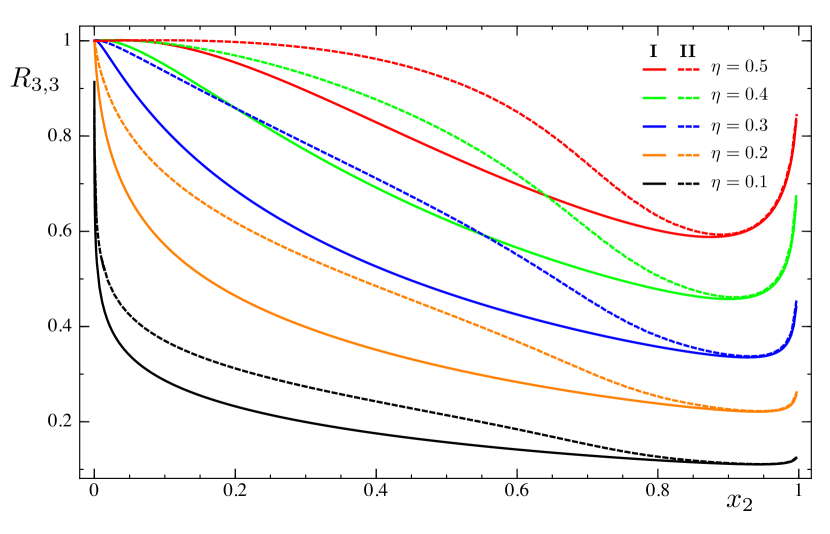
Figure 6: The function $R_{3,3}(\boldsymbol{x})$ for the free compactified boson, obtained from (2.21) and (3.29), computed for two configurations of intervals defined in §5 (see Fig. 3).

Given the period matrix $\tau$ for $\mathscr{R}_{N,n}$ computed in §3.1, the quantum and the classical part in $\mathcal{F}_{N,n}(\boldsymbol{x})=\mathcal{F}_{N,n}^{\textrm{\tiny qu}}\,\mathcal{F}_{N,n}^{\textrm{\tiny cl}}(\eta)$ read [7, 9, 10, 14]

$$\mathcal{F}_{N,n}^{\textrm{\tiny qu}}=\frac{1}{|\Theta(\boldsymbol{0}|\tau)|^{2}}\,,\qquad\mathcal{F}_{N,n}^{\textrm{\tiny cl}}(\eta)=\sum_{\boldsymbol{p},\tilde{\boldsymbol{p}}}\exp[\textrm{i}\pi(\boldsymbol{p}^{{\rm t}}\cdot\tau\cdot\boldsymbol{p}-\tilde{\boldsymbol{p}}^{{\rm t}}\cdot\tau\cdot\tilde{\boldsymbol{p}})]\,,$$ (3.23)

where

$$\boldsymbol{p}=\frac{\boldsymbol{m}}{\sqrt{2\eta}}+\frac{\boldsymbol{n}\sqrt{2\eta}}{2}\,,\qquad\tilde{\boldsymbol{p}}=\frac{\boldsymbol{m}}{\sqrt{2\eta}}-\frac{\boldsymbol{n}\sqrt{2\eta}}{2}\,,\qquad\boldsymbol{m},\boldsymbol{n}\in\mathbb{Z}^{g}\,.$$ (3.24)

Expanding the argument of the exponential in (3.23), one finds that the classical part can be written in terms of the Riemann theta function as

$$\mathcal{F}_{N,n}^{\textrm{\tiny cl}}(\eta)=\Theta(\boldsymbol{0}|T_{\eta})\,,$$ (3.25)

where $T_{\eta}$ is the following $2g\times 2g$ symmetric matrix

$$T_{\eta}=\begin{pmatrix}\,{\rm i}\,\eta\,\mathcal{I}&\mathcal{R}\\ \mathcal{R}&{\rm i}\,\mathcal{I}/\eta\,\end{pmatrix}.$$ (3.26)

Being $\mathcal{I}$ positive definite and $\eta>0$, also the imaginary part of $T_{\eta}$ is positive definite. From (3.25) and (3.26), it is straightforward to observe that $\mathcal{F}^{{\rm cl}}_{N,n}(\eta)=\mathcal{F}^{{\rm cl}}_{N,n}(1/\eta)$. Thus, since all the dependence of $\mathcal{F}_{N,n}(\boldsymbol{x})$ on $\eta$ is contained in $\mathcal{F}^{{\rm cl}}_{N,n}$, we find that $\mathcal{F}_{N,n}(\boldsymbol{x})$ is invariant under $\eta\leftrightarrow 1/\eta$.

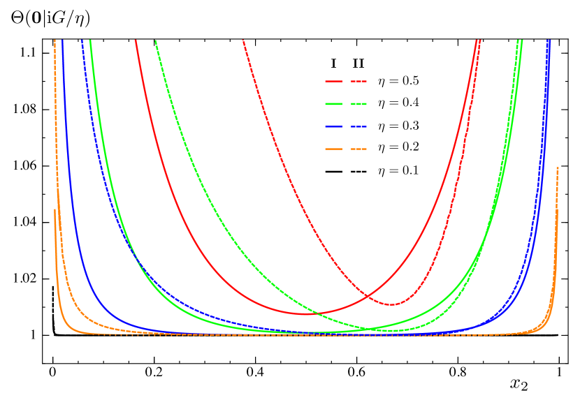
Figure 7: The function $\Theta(\boldsymbol{0}|\textrm{i}G/\eta)$ with $N=3$, $n=3$ and for the configurations I and II shown in Fig. 3. For small $\eta$ (the decompactification regime) this term can be neglected (see (3.27) and (3.29)).

By employing the Poisson summation formula (only for half of the sums), the classical part (3.25) can be written as

$$\mathcal{F}_{N,n}^{\textrm{\tiny cl}}(\eta)=\eta^{g/2}\,\frac{\Theta(\boldsymbol{0}|\textrm{i}\eta G)}{\sqrt{\textrm{det}(\mathcal{I})}}=\eta^{-g/2}\,\frac{\Theta(\boldsymbol{0}|\textrm{i}G/\eta)}{\sqrt{\textrm{det}(\mathcal{I})}}\,,$$ (3.27)

where the $g\times g$ matrix $G$ reads

$$G=\begin{pmatrix}\,\mathcal{I}+\mathcal{R}\cdot\mathcal{I}^{-1}\cdot\mathcal{R}&\;\;\mathcal{R}\cdot\mathcal{I}^{-1}\,\\ \mathcal{I}^{-1}\cdot\mathcal{R}&\;\;\mathcal{I}^{-1}\end{pmatrix}.$$ (3.28)

This matrix is real, independent of $\eta$ and symmetric, being $\mathcal{R}$ and $\mathcal{I}$ symmetric matrices.
Combining (3.23), (3.25) and (3.27), we find $\mathcal{F}_{N,n}(\boldsymbol{x})$ for the free compactified boson

$$\mathcal{F}_{N,n}(\boldsymbol{x})=\frac{\Theta(\boldsymbol{0}|T_{\eta})}{|\Theta(\boldsymbol{0}|\tau)|^{2}}=\frac{\eta^{g/2}\,\Theta(\boldsymbol{0}|\textrm{i}\eta G)}{\sqrt{\textrm{det}(\mathcal{I})}\,|\Theta(\boldsymbol{0}|\tau)|^{2}}=\frac{\eta^{-g/2}\,\Theta(\boldsymbol{0}|\textrm{i}G/\eta)}{\sqrt{\textrm{det}(\mathcal{I})}\,|\Theta(\boldsymbol{0}|\tau)|^{2}}\,.$$ (3.29)

The term $|\Theta(\boldsymbol{0}|\tau)|$ in the denominator can be rewritten by applying the Thomae type formula for the complex curves (3.3) [30, 55]

$$\Theta(\boldsymbol{0}|\tau)^{8}=\frac{\prod_{k\,=1}^{n-1}[\textrm{det}(\mathcal{A}_{k})]^{4}}{(2\pi\textrm{i})^{4g}}\,\Bigg{(}\,\prod_{\begin{subarray}{c}i,j\,=\,0\\ i\,<\,j\end{subarray}}^{N-1}(x_{2j}-x_{2i})\prod_{\begin{subarray}{c}r,s\,=\,0\\ r\,<\,s\end{subarray}}^{N-2}(x_{2s+1}-x_{2r+1})\Bigg{)}^{2(n-1)},$$ (3.30)

where the $(N-1)\times(N-1)$ matrices $\mathcal{A}_{k}$ have been defined in (3.18).
Plugging (3.29) into (2.7), one finds ${\rm Tr}\rho_{A}^{n}$ for the free compactified boson in terms of the compactification radius and of the endpoints of the intervals. Once $\mathcal{F}_{N,n}(\boldsymbol{x})$ has been found, $\tilde{R}_{N,n}(\boldsymbol{x})$ and $R_{N,n}(\boldsymbol{x})$ are obtained through (2.17) and (2.21) respectively.

In [6] the expansion where all the lengths of the intervals are small with respect to the other characteristic lengths of the systems has been studied. This means that $x_{2i+1}-x_{2i}$ are small compared to the distances $x_{2j+2}-x_{2j+1}$, where $i,j=0,\dots,N-2$ (we recall that $x_{0}=0$ and $x_{2N-2}=1$). Analytic expressions have been found for $N=2$ [6] and one could extend this analysis to $N>2$ by employing (3.29). We leave this analysis for future work. We checked numerically that $\mathcal{F}_{N,n}(\boldsymbol{0})=1$, which generalizes the known result $\mathcal{F}_{2,n}(0)=1$ [5].

In Appendix C we discuss the invariance of (3.29) under a cyclic change in the ordering of the sheets, an inversion and the exchange $A\leftrightarrow B$, writing explicitly these transformations in terms of symplectic matrices.

3.3 The decompactification regime

When $\eta\rightarrow\infty$ the target space of the free boson becomes the infinite line. This regime is important because it can be obtained as the continuum limit of the harmonic chain. Notice that the results of this subsection can be obtained also for $\eta\rightarrow 0$ because of the $\eta\leftrightarrow 1/\eta$ invariance.

Since $\Theta(\boldsymbol{0}|\textrm{i}\eta G)\rightarrow 1$ when $\eta\rightarrow\infty$ (or equivalently $\Theta(\boldsymbol{0}|\textrm{i}G/\eta)\rightarrow 1$ when $\eta\rightarrow 0$ as shown in Fig. 7), we find that (3.29) becomes

$$\mathcal{F}_{N,n}^{\eta\rightarrow\infty}(\boldsymbol{x})=\frac{\eta^{g/2}}{\sqrt{\textrm{det}(\mathcal{I})}\,|\Theta(\boldsymbol{0}|\tau)|^{2}}\equiv\eta^{g/2}\,\widehat{\mathcal{F}}_{N,n}(\boldsymbol{x})\,.$$ (3.31)

Writing $|\Theta(\boldsymbol{0}|\tau)|$ through (3.30), one can improve the numerical evaluation of (3.31).
Plugging (3.31) into (2.21), we find that in the decompactification regime $R_{N,n}$ becomes

$$R_{N,n}^{\eta\rightarrow\infty}(\boldsymbol{x})=\eta^{(-1)^{N}(n-1)/2}\prod_{p\,=\,2}^{N}\,\prod_{\sigma_{N,p}}\big{[}\widehat{\mathcal{F}}_{p,n}(\boldsymbol{x}^{\sigma_{N,p}})\big{]}^{(-1)^{N-p}}\,.$$ (3.32)

In this case it is very useful to consider the normalization (2.23) through a fixed configuration of intervals characterized by $\boldsymbol{x}_{\textrm{\tiny{fixed}}}$ because the dependence on $\eta$ simplifies in the ratio. Indeed, from (3.32) we find

$$\lim_{\eta\,\rightarrow\,\infty}R_{N,n}^{\textrm{\tiny{norm}}}(\boldsymbol{x})=\frac{R_{N,n}^{\eta\rightarrow\infty}(\boldsymbol{x})}{R_{N,n}^{\eta\rightarrow\infty}(\boldsymbol{x}_{\textrm{\tiny{fixed}}})}=\prod_{p\,=\,2}^{N}\,\prod_{\sigma_{N,p}}\left[\frac{\widehat{\mathcal{F}}_{p,n}(\boldsymbol{x}^{\sigma_{N,p}})}{\widehat{\mathcal{F}}_{p,n}(\boldsymbol{x}^{\sigma_{N,p}}_{\textrm{\tiny{fixed}}})}\right]^{(-1)^{N-p}},$$ (3.33)

and similarly, from (3.31), we have

$$\lim_{\eta\,\rightarrow\,\infty}\mathcal{F}_{N,n}^{\textrm{\tiny{norm}}}(\boldsymbol{x})=\frac{\mathcal{F}_{N,n}^{\eta\rightarrow\infty}(\boldsymbol{x})}{\mathcal{F}_{N,n}^{\eta\rightarrow\infty}(\boldsymbol{x}_{\textrm{\tiny{fixed}}})}=\frac{\widehat{\mathcal{F}}_{N,n}(\boldsymbol{x})}{\widehat{\mathcal{F}}_{N,n}(\boldsymbol{x}_{\textrm{\tiny{fixed}}})}\,.$$ (3.34)

In §5 we compare (3.33) and (3.34) to the corresponding results for the harmonic chain with periodic boundary conditions.

3.4 The Dirac model

It is well known that the partition function of the compactified massless free boson describes various systems at criticality. For example, the free Dirac fermion corresponds to the case $\eta=1/2$. Given (3.29), we can write ${\rm Tr}\rho_{A}^{n}$ for this model by applying the results of [9, 10, 11, 14]. Let us introduce the Riemann theta function with characteristic $\boldsymbol{e}^{{\rm t}}=(\boldsymbol{\varepsilon}^{{\rm t}},\boldsymbol{\delta}^{{\rm t}})$, namely

$$\Theta[\boldsymbol{e}](\boldsymbol{z}|\Omega)=\sum_{\boldsymbol{m}\,\in\,\mathbb{Z}^{p}}\exp\big{[}\textrm{i}\pi(\boldsymbol{m}+\boldsymbol{\varepsilon})^{{\rm t}}\cdot\Omega\cdot(\boldsymbol{m}+\boldsymbol{\varepsilon})+2\pi\textrm{i}(\boldsymbol{m}+\boldsymbol{\varepsilon})^{{\rm t}}\cdot(\boldsymbol{z}+\boldsymbol{\delta})\big{]}\,,$$ (3.35)

where $\boldsymbol{z}\in\mathbb{C}^{p}/(\mathbb{Z}^{p}+\tau\,\mathbb{Z}^{p})$ is the independent variable, while $\boldsymbol{\varepsilon}$ and $\boldsymbol{\delta}$ are vectors whose entries are either 0 or $1/2$. When $\boldsymbol{\varepsilon}=\boldsymbol{\delta}=\boldsymbol{0}$ and $\boldsymbol{z}=\boldsymbol{0}$, we recover (3.22). The parity of (3.35) is the same one of the integer number $4\boldsymbol{\varepsilon}\cdot\boldsymbol{\delta}$; indeed

$$\Theta[\boldsymbol{e}](-\boldsymbol{z}|\Omega)=(-1)^{4\boldsymbol{\varepsilon}\cdot\boldsymbol{\delta}}\,\Theta[\boldsymbol{e}](\boldsymbol{z}|\Omega)\,.$$ (3.36)

The characteristics $\boldsymbol{e}$ are either even or odd, according to the parity of $4\boldsymbol{\varepsilon}\cdot\boldsymbol{\delta}$. It is not difficult to realize that there are $2^{p-1}(2^{p}+1)$ even characteristics, $2^{p-1}(2^{p}-1)$ odd ones.

Applying some identities for the Riemann theta functions, from (3.29) one finds

$$\mathcal{F}^{\textrm{\tiny Dirac}}_{N,n}(\boldsymbol{x})=\mathcal{F}_{N,n}(\boldsymbol{x})\big{|}_{\eta=1/2}=\frac{\sum_{\boldsymbol{e}}|\Theta[\boldsymbol{e}](\boldsymbol{0}|\tau)|^{2}}{2^{g}\,|\Theta(\boldsymbol{0}|\tau)|^{2}}\,,$$ (3.37)

where the period matrix $\tau$ has been computed in §3.1. Notice that, being $\Theta[\boldsymbol{e}](\boldsymbol{0}|\Omega)=0$ when $\boldsymbol{e}$ is odd, in the sum over the characteristics in (3.37) only the even ones occur. Since (3.37) has been obtained as the special case $\eta=1/2$ of (3.29), $\mathcal{F}^{\textrm{\tiny Dirac}}_{N,n}(\boldsymbol{0})=1$. The result of [26] corresponds to keep only $\boldsymbol{e}=\boldsymbol{0}$ in the numerator of (3.37) instead of considering the sum over all the sectors of the model. We refer the reader to [29] for a detailed comparison between these two approaches.

4 Recovering the two intervals case

It is not straightforward to recover the known results for two intervals [5, 6], whose generalization allowed to study the partial transposition and the negativity for a two dimensional CFT [35, 36]. In this section we first review the status of the two intervals case and then we show that the corresponding Rényi entropies reduce to a particular case of the expressions discussed in §3, as expected.

4.1 Two disjoint intervals and partial transposition

The negativity [33] provides a good measure of entanglement for mixed states. Considering a bipartition where $A$ is made by two disjoint intervals, the negativity can be found as a replica limit $n_{e}\rightarrow 1$ of ${\rm Tr}(\rho_{A}^{T_{A_{2}}})^{n_{e}}$ where $n_{e}$ is an even number and $\rho_{A}^{T_{A_{2}}}$ is obtained by taking $\rho_{A}$ and partially transpose it with respect to the second interval. For a two dimensional CFT, it turns out that ${\rm Tr}(\rho_{A}^{T_{A_{2}}})^{n}$ is obtained by considering the four point function $\langle\mathcal{T}_{n}\bar{\mathcal{T}}_{n}\mathcal{T}_{n}\bar{\mathcal{T}}_{n}\rangle$, and exchanging the twist fields $\mathcal{T}_{n}$ and $\bar{\mathcal{T}}_{n}$ at the endpoints af $A_{2}$. In terms of the harmonic ratio $x$ of the four points, while for the Rényi entropies it is enough to consider $x\in(0,1)$, the partial transposition forces us to include also the range $x<0$. For generic positions of the twist fields in the complex plane, $x\in\mathbb{C}$ and the corresponding expression of $\langle\mathcal{T}_{n}\bar{\mathcal{T}}_{n}\mathcal{T}_{n}\bar{\mathcal{T}}_{n}\rangle$ is given by the r.h.s. of (2.7) with $\mathcal{F}_{2,n}=\mathcal{F}_{2,n}(x,\bar{x})$.

For the free compactified boson, this function reads [36]

$$\mathcal{F}_{2,n}(x,\bar{x})=\frac{\Theta(\boldsymbol{0}|T_{\eta,2})}{\prod_{k=1}^{n-1}|F_{k/n}(x)|}=\frac{\Theta(\boldsymbol{0}|T_{\eta,2})}{|\Theta(\boldsymbol{0}|\tau_{2})|^{2}}\,,\qquad F_{k/n}(x)\equiv\,_{2}F_{1}(k/n,1-k/n;1;x)\,,$$ (4.1)

where $T_{\eta,2}$ is the $2(n-1)\times 2(n-1)$ symmetric matrix given by

$$T_{\eta,2}=\begin{pmatrix}\,{\rm i}\,\eta\,\textrm{Im}(\tau_{2})&\textrm{Re}(\tau_{2})\\ \textrm{Re}(\tau_{2})&{\rm i}\,\textrm{Im}(\tau_{2})/\eta\,\end{pmatrix},$$ (4.2)

defined in terms of the following $(n-1)\times(n-1)$ complex and symmetric matrix

$$(\tau_{2})_{ij}=\frac{2}{n}\sum_{k=1}^{n-1}\sin(\pi k/n)\bigg{[}\,\textrm{i}\,\frac{F_{k/n}(1-x)}{F_{k/n}(x)}\,\bigg{]}\cos[2\pi k/n(i-j)]\,.$$ (4.3)

The matrix $T_{\eta,2}$ in (4.1) is defined as in (3.26) with $\tau_{2}$ instead of $\tau$. In the second step of (4.1) the Thomae formula (3.30) has been employed. Notice that, because of the sum over $k$ in (4.3), substituting $\cos[2\pi k/n(i-j)]$ with $\rho_{n}^{k(i-j)}$ the matrix does not change. The non vanishing of $\textrm{Re}(\tau_{2})$ is due to the fact that the term within the square brackets in (4.3) is complex for $x\in\mathbb{C}$.

As briefly explained in §3.4, it is straightforward to write the corresponding result for the Dirac model from (4.1). It reads

$$\mathcal{F}^{\textrm{\tiny Dirac}}_{2,n}(x,\bar{x})=\frac{\sum_{\boldsymbol{e}}|\Theta[\boldsymbol{e}](\boldsymbol{0}|\tau_{2})|^{2}}{2^{n-1}\,|\Theta(\boldsymbol{0}|\tau_{2})|^{2}}\,.$$ (4.4)

Given the period matrix (4.3), one can also find $\mathcal{F}^{\textrm{\tiny Ising}}_{2,n}(x,\bar{x})$ for the Ising model [38, 39]

$$\mathcal{F}^{\textrm{\tiny Ising}}_{2,n}(x,\bar{x})=\frac{\sum_{\boldsymbol{e}}|\Theta[\boldsymbol{e}](\boldsymbol{0}|\tau_{2})|}{2^{n-1}\,|\Theta(\boldsymbol{0}|\tau_{2})|}\,.$$ (4.5)

In order to consider the Rényi entropies, we must restrict to $x\in(0,1)$. Within this domain, $F_{k/n}(x)$ is real and this leads to a purely imaginary $\tau_{2}$. Since $\textrm{Re}(\tau_{2})$ vanishes identically for $x\in(0,1)$, the matrix $T_{\eta,2}$ in (4.2) becomes block diagonal and therefore $\Theta(\boldsymbol{0}|T_{\eta,2})=\Theta(\boldsymbol{0}|\,{\rm i}\eta\,\textrm{Im}(\tau_{2}))\,\Theta(\boldsymbol{0}|\,{\rm i}\,\textrm{Im}(\tau_{2})/\eta)$ factorizes. Thus, the expressions given in (4.1) and (4.5) reduce to $\mathcal{F}_{2,n}(x)$ for the free compactified boson [5] and for the Ising model [6] respectively.

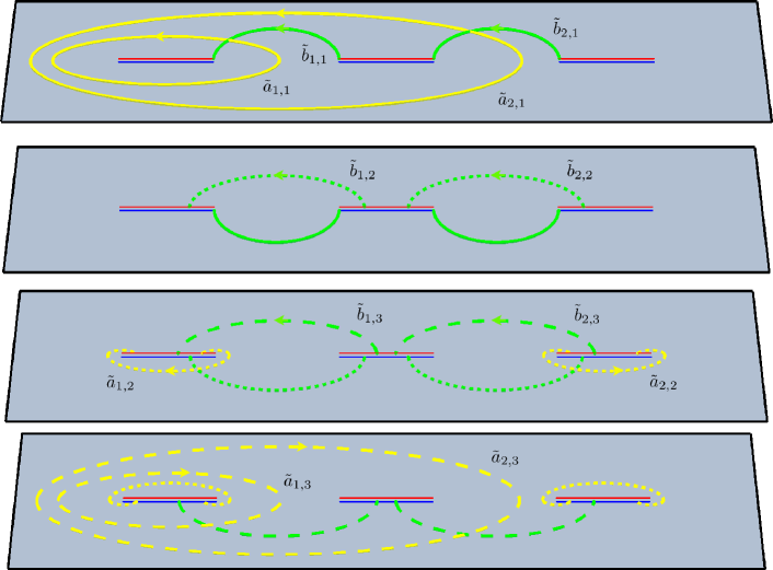
Figure 8: The canonical homology basis $\{\tilde{a}_{\alpha,j},\tilde{b}_{\alpha,j}\}$ for $N=3$ and $n=4$.

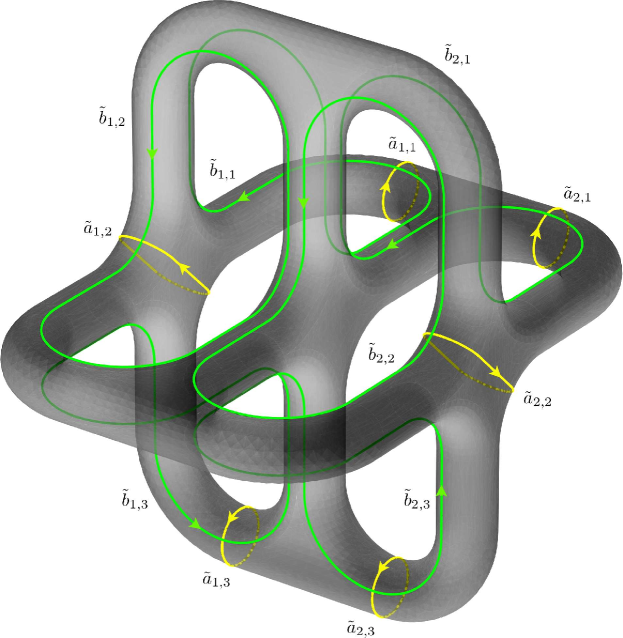
Figure 9: The Riemann surface $\mathscr{R}_{3,4}$ with the canonical homology basis $\{\tilde{a}_{\alpha,j},\tilde{b}_{\alpha,j}\}$.

4.2 Another canonical homology basis

To recover the period matrix (4.3) for $x\in(0,1)$ as the two intervals case of a period matrix characterizing $N\geqslant 2$ intervals, we find it useful to introduce the canonical homology basis $\{\tilde{a}_{\alpha,j},\tilde{b}_{\alpha,j}\}$ depicted in Figs. 8 and 9. This basis is considered very often in the literature on higher genus Riemann surfaces (e.g. see Fig. 1 both in [9] and [10]). Integrating the holomorphic differentials (3.4) along the cycles $\tilde{\boldsymbol{a}}$ and $\tilde{\boldsymbol{b}}$, as done in (3.5) for the untilded ones, one gets the matrices $\tilde{\mathcal{A}}$ and $\tilde{\mathcal{B}}$. To evaluate these matrices, we repeat the procedure described in §3.1. In particular, we first write $\{\tilde{a}_{\alpha,j},\tilde{b}_{\alpha,j}\}$ through the auxiliary cycles depicted in Figs. 27 and 28, finding that

$$\tilde{a}_{\alpha,j}=\sum_{\gamma=1}^{\alpha}\sum_{l=1}^{j}a^{\textrm{\tiny aux}}_{\gamma,l}\,,\qquad\tilde{b}_{\alpha,j}=b^{\textrm{\tiny aux}}_{\alpha,j}\,.$$ (4.6)

Comparing (3.8) with (4.6), we observe that for $n=2$ the canonical homology basis introduced here coincides with the one defined in §3.1. From (4.6), one can write the matrices $\tilde{\mathcal{A}}$ and $\tilde{\mathcal{B}}$ as follows

$$\tilde{\mathcal{A}}^{\beta,\alpha}_{k,j}=\sum_{\gamma=1}^{\alpha}\sum_{l=1}^{j}(\mathcal{A}^{\textrm{\tiny aux}})^{\beta,\gamma}_{k,l}=\sum_{\gamma=1}^{\alpha}\sum_{l=1}^{j}\rho_{n}^{k(l-1)}(\mathcal{A}^{\textrm{\tiny aux}})^{\beta,\gamma}_{k,1}=\frac{1-\rho_{n}^{jk}}{1-\rho_{n}^{k}}\,\sum_{\gamma=1}^{\alpha}(\mathcal{A}^{\textrm{\tiny aux}})^{\beta,\gamma}_{k,1}\,,$$ (4.7)

$$\tilde{\mathcal{B}}^{\beta,\alpha}_{k,j}=(\mathcal{B}^{\textrm{\tiny aux}})^{\beta,\alpha}_{k,j}=\rho_{n}^{k(j-1)}(\mathcal{B}^{\textrm{\tiny aux}})^{\beta,\alpha}_{k,1}\,,$$ (4.8)

where (3.9) has been used. Now the elements of $\tilde{\mathcal{A}}$ and $\tilde{\mathcal{B}}$ are expressed in terms of the integrals (3.12) and (3.13), which can be numerically evaluated. Once $\tilde{\mathcal{A}}$ and $\tilde{\mathcal{B}}$ have been computed, the period matrix with respect to the basis $\{\tilde{a}_{\alpha,j},\tilde{b}_{\alpha,j}\}$ is $\tilde{\tau}=\tilde{\mathcal{A}}^{-1}\cdot\tilde{\mathcal{B}}$.

Since the matrices $\tilde{\mathcal{A}}$ and $\tilde{\mathcal{B}}$ have the structure (3.15), like $\mathcal{A}$ and $\mathcal{B}$ in §3.1, we can write them as in (3.16) with

$$(\mathscr{M}_{\tilde{\mathcal{A}}})_{kj} \equiv \frac{1-\rho_{n}^{kj}}{1-\rho_{n}^{k}}\,,\qquad\hskip 22.76228pt(\tilde{\mathcal{A}}_{k})_{\beta\alpha}\equiv\tilde{\mathcal{A}}^{\beta,\alpha}_{k,1}=(\rho_{n}^{-k}-1)\sum_{\gamma\,=\,1}^{\alpha}(-1)^{N-\gamma}\mathscr{I}_{\beta,k}\big{|}_{x_{2\gamma-2}}^{x_{2\gamma-1}}\,$$ (4.9)

$$(\mathscr{M}_{\tilde{\mathcal{B}}})_{kj} \equiv \rho_{n}^{k(j-1)}\,,\qquad\hskip 29.02193pt(\tilde{\mathcal{B}}_{k})_{\beta\alpha}\equiv\tilde{\mathcal{B}}^{\beta,\alpha}_{k,1}=(-1)^{N-\alpha}\rho_{n}^{k/2}(\rho_{n}^{-k}-1)\,\mathscr{I}_{\beta,k}\big{|}_{x_{2\alpha-1}}^{x_{2\alpha}}\,.$$ (4.10)

where (3.12) and (3.13) have been employed and $\mathscr{I}_{\beta,k}\big{|}_{b}^{a}$ are the integrals (3.14). Notice that $\tilde{\mathcal{A}}_{k}=\mathcal{A}_{k}$, while $(\tilde{\mathcal{B}}_{k})_{\beta\alpha}=(\mathcal{B}^{\textrm{\tiny aux}})^{\beta,\alpha}_{k,1}=-\rho_{n}^{k}(\mathcal{B}_{k})_{\beta\alpha}$. Thus, the period matrix $\tilde{\tau}$ reads

$$\tilde{\tau}=(\mathscr{M}_{\tilde{\mathcal{A}}}\otimes\mathbb{I}_{N-1})^{-1}\cdot\textrm{diag}(\tilde{\mathcal{A}}^{-1}_{1}\cdot\tilde{\mathcal{B}}_{1},\tilde{\mathcal{A}}^{-1}_{2}\cdot\tilde{\mathcal{B}}_{2},\dots,\tilde{\mathcal{A}}^{-1}_{n-1}\cdot\tilde{\mathcal{B}}_{n-1})\cdot(\mathscr{M}_{\tilde{\mathcal{B}}}\otimes\mathbb{I}_{N-1})\,.$$ (4.11)

Since (3.20) and (4.11) are the period matrices of the Riemann surface $\mathscr{R}_{N,n}$ with respect to different canonical homology bases, they must be related through a symplectic transformation. The relations (3.8) and (4.6) in the matrix form become respectively

$$\left\{\begin{array}[]{l}\boldsymbol{a}=A\cdot\boldsymbol{a}^{\textrm{\tiny aux}}\\ \boldsymbol{b}=B\cdot\boldsymbol{b}^{\textrm{\tiny aux}}\end{array}\right.,\qquad\left\{\begin{array}[]{l}\tilde{\boldsymbol{a}}=\tilde{A}\cdot\boldsymbol{a}^{\textrm{\tiny aux}}\\ \tilde{\boldsymbol{b}}=\boldsymbol{b}^{\textrm{\tiny aux}}\end{array}\right..$$ (4.12)

Introducing the $p\times p$ upper triangular matrix $I_{p}^{\textrm{\tiny up}}$ made by $1$’s (i.e. $(I_{p}^{\textrm{\tiny up}})_{ab}=1$ if $a\leqslant b$ and zero otherwise) and also its transposed $I_{p}^{\textrm{\tiny low}}\equiv(I_{p}^{\textrm{\tiny up}})^{\textrm{t}}$, which is a lower triangular matrix, we can write that $A=\mathbb{I}_{n-1}\otimes I_{N-1}^{\textrm{\tiny low}}$, $B=I_{n-1}^{\textrm{\tiny up}}\otimes\mathbb{I}_{N-1}$ and $\tilde{A}=I_{n-1}^{\textrm{\tiny low}}\otimes I_{N-1}^{\textrm{\tiny low}}$. We remark that the matrices $\textrm{diag}(A,B)$ and $\textrm{diag}(\tilde{A},\mathbb{I}_{g})$ occurring in (4.12) are not symplectic matrices because, as already noticed in §3.1, the auxiliary set of cycles is not a canonical homology basis. From (4.12) it is straightforward to find the relation between the two canonical homology bases, namely

$$\left\{\begin{array}[]{l}\tilde{\boldsymbol{a}}=\tilde{A}\cdot A^{-1}\cdot\boldsymbol{a}\\ \tilde{\boldsymbol{b}}=B^{-1}\cdot\boldsymbol{b}\end{array}\right.,\qquad M\equiv\begin{pmatrix}\tilde{A}\cdot A^{-1}&0_{g}\\ 0_{g}&B^{-1}\end{pmatrix}\in Sp(2g,\mathbb{Z})\,,$$ (4.13)

which can be constructed by using that $(I_{p}^{\textrm{\tiny up}})_{ab}^{-1}=\delta_{a,b}-\delta_{a+1,b}$ and the properties of the tensor product, finding $\tilde{A}\cdot A^{-1}=I_{n-1}^{\textrm{\tiny low}}\otimes\mathbb{I}_{N-1}$ and $B^{-1}=(I_{n-1}^{\textrm{\tiny up}})^{-1}\otimes\mathbb{I}_{N-1}$. Notice that (4.13) belongs to the symplectic modular group, as expected from the fact that it encodes the change between canonical homology bases.

4.3 The case $N=2$

Specializing the expressions given in the previous subsection to the $N=2$ case, the greek indices assume only a single value; therefore they can be suppressed. The matrices (4.7) and (4.8) become respectively

$$\tilde{\mathcal{A}}_{kj} \equiv \tilde{\mathcal{A}}^{1,1}_{k,j}=\frac{1-\rho_{n}^{jk}}{1-\rho_{n}^{k}}\Big{[}(1-\rho_{n}^{-k})\mathscr{I}_{1,k}\big{|}_{0}^{x}\,\Big{]}=\frac{1-\rho_{n}^{kj}}{1-\rho_{n}^{k}}\big{[}2\pi\textrm{i}\,\rho_{n}^{-k/2}F_{k/n}(x)\big{]}\,,$$ (4.14)

$$\rule{0.0pt}{17.07182pt}\tilde{\mathcal{B}}_{kj} \equiv \tilde{\mathcal{B}}^{1,1}_{k,j}=\rho_{n}^{k(j-1)}\Big{[}\rho_{n}^{k/2}(1-\rho_{n}^{-k})\mathscr{I}_{1,k}\big{|}_{x}^{1}\,\Big{]}=\rho_{n}^{k(j-1)}\big{[}2\pi\textrm{i}\,F_{k/n}(1-x)\big{]}\,,$$ (4.15)

where $x\in(0,1)$, the indices $j,k\in\{1,\dots,n-1\}$ and the explicit results for $(\mathcal{A}^{\textrm{\tiny aux}})_{k,1}$ and $(\mathcal{B}^{\textrm{\tiny aux}})_{k,1}$, from (3.12) and (3.13) respectively, are written within the square brackets (see (4.29) of [8] and also (B.7) and (B.8)). The matrices (4.14) and (4.15) can be written respectively as follow

$$\tilde{\mathcal{A}} = \textrm{diag}(\dots,2\pi\textrm{i}\,\rho_{n}^{-k/2}F_{k/n}(x),\dots)\cdot\mathscr{M}_{\tilde{\mathcal{A}}}\,,$$ (4.16)

$$\rule{0.0pt}{14.22636pt}\tilde{\mathcal{B}} = \textrm{diag}(\dots,2\pi\textrm{i}\,F_{k/n}(1-x),\dots)\cdot\mathscr{M}_{\tilde{\mathcal{B}}}\,,$$ (4.17)

where $\mathscr{M}_{\tilde{\mathcal{A}}}$ and $\mathscr{M}_{\tilde{\mathcal{B}}}$ have been defined in (4.9) and (4.10) respectively. Computing $\mathscr{M}_{\tilde{\mathcal{A}}}^{-1}$, whose elements read $(\mathscr{M}_{\tilde{\mathcal{A}}}^{-1})_{ik}=(\rho_{n}^{k}-1)/(n\rho_{n}^{ik})$, we can easily check that (4.3) becomes

$$\tau_{2}=\tilde{\mathcal{A}}^{-1}\cdot\tilde{\mathcal{B}}=\mathscr{M}_{\tilde{\mathcal{A}}}^{-1}\cdot\textrm{diag}\bigg{(}\dots,\,\rho_{n}^{k/2}\,\frac{F_{k/n}(1-x)}{F_{k/n}(x)}\,,\,\dots\bigg{)}\cdot\mathscr{M}_{\tilde{\mathcal{B}}}\,.$$ (4.18)

Thus, the matrix (4.3) for $0<x<1$, found in [5], is the $N=2$ case of the period matrix $\tilde{\tau}$, written with respect to the canonical homology basis introduced in the section §4.2

$$\tilde{\tau}|_{N=2}=\tau_{2}\,.$$ (4.19)

To conclude this section, let us consider the symplectic transformation (4.13), which reduces to $\textrm{diag}(I_{n-1}^{\textrm{\tiny low}},(I_{n-1}^{\textrm{\tiny up}})^{-1})$ for $N=2$. Its inverse reads $\textrm{diag}((I_{n-1}^{\textrm{\tiny low}})^{-1},I_{n-1}^{\textrm{\tiny up}})$ and it allows us to find the period matrix $\tau_{2}^{\prime}$ with respect to the canonical homology basis given by the cycles $\boldsymbol{a}$ and $\boldsymbol{b}$ through (C.3), namely

$$\tau_{2}^{\prime}=I_{n-1}^{\textrm{\tiny up}}\cdot\tau_{2}\cdot I_{n-1}^{\textrm{\tiny low}}\,.$$ (4.20)

Introducing the symmetric matrix $\mathscr{A}_{ij}\equiv 2/n\sum_{k=1}^{n-1}\sin(\pi k/n)\,e^{2\pi\textrm{i}(j-i)}$ (which has been denoted by $A$ in the Appendix C of [5]), after some algebra we find

$$\mathscr{A}\cdot I_{n-1}^{\textrm{\tiny up}}\cdot\tau_{2}\cdot I_{n-1}^{\textrm{\tiny low}}\cdot\mathscr{A}=\,\tau_{2}\,.$$ (4.21)

Combining (4.20) and (4.21), we easily get that $\tau_{2}^{\prime}=\mathscr{A}^{-1}\cdot\tau_{2}\cdot\mathscr{A}^{-1}$. Then, by employing (C.7) and the fact that $\textrm{det}(I_{n-1}^{\textrm{\tiny up}})=1$, we get

$$\Theta(\boldsymbol{0}|\tau_{2}^{\prime})=\Theta(\boldsymbol{0}|\mathscr{A}^{-1}\cdot\tau_{2}\cdot\mathscr{A}^{-1})=\Theta(\boldsymbol{0}|\tau_{2})\,.$$ (4.22)

In [5] the second equality in (4.22) has been given as a numerical observation. We have shown that it is a consequence of the relation between the two canonical homology bases considered here.

5 The harmonic chain

In this section we consider the Rényi entropies and the entanglement entropy for the harmonic chain with periodic boundary conditions, which have been largely studied in the literature [56, 57, 58, 59, 60, 61, 62]. We compute new data for the case of disjoint blocks in order to check the CFT formulas found in §3 for the decompactification regime.

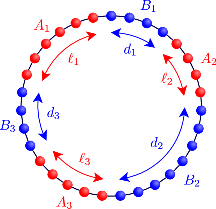
Figure 10: A bipartition of the periodic chain where $A$ is made by the union of three disjoint blocks of lattice sites.

The Hamiltonian of the harmonic chain made by $L$ lattice sites and with nearest neighbor interaction reads

$$H=\sum_{n=0}^{L-1}\left(\frac{1}{2M}\,p_{n}^{2}+\frac{M\omega^{2}}{2}\,q_{n}^{2}+\frac{K}{2}(q_{n+1}-q_{n})^{2}\right),$$ (5.1)

where periodic boundary conditions $q_{0}=q_{L}$ and $p_{0}=p_{L}$ are imposed and the variables $q_{n}$ and $p_{m}$ satisfy the commutation relations $[q_{n},q_{m}]=[p_{n},p_{m}]=0$ and $[q_{n},p_{m}]=\textrm{i}\delta_{n,m}$. The Hamiltonian (5.1) contains three parameters $\omega$, $M$, $K$ but, through a canonical rescaling of the variables, it can be written in a form where these parameters occur only in a global factor and in the coupling $\tfrac{2K}{M\omega^{2}}/(1+\tfrac{2K}{M\omega^{2}})$ [34, 58]. The Hamiltonian (5.1) is the lattice discretization of a free massive boson. When $\omega=0$ the theory is conformal with central charge $c=1$. Since the bosonic field is not compactified, we must compare the continuum limit of (5.1) for $\omega=0$ with the regime $\eta\rightarrow\infty$ of the CFT expressions computed in §3, which has been considered in §3.3.

To diagonalize (5.1), first one exploits the translational invariance of the system by Fourier transforming $q_{n}$ and $p_{n}$. Then the annihilation and creation operators $a_{k}$ and $a_{k}^{\dagger}$ are introduced, whose algebra is $[a_{k},a_{k^{\prime}}]=[a_{k}^{\dagger},a_{k^{\prime}}^{\dagger}]=0$ and $[a_{k},a_{k^{\prime}}^{\dagger}]=\textrm{i}\delta_{k,k^{\prime}}$. The ground state of the system $|0\rangle$ is annihilated by all the $a_{k}$’s and it is a pure Gaussian state. In terms of the annihilation and creation operators, the Hamiltonian (5.1) is diagonal

$$H=\sum_{k=0}^{L-1}\omega_{k}\left(a^{\dagger}_{k}a_{k}+\frac{1}{2}\right),$$ (5.2)

where

$$\omega_{k}\equiv\sqrt{\omega^{2}+\frac{4K}{M}\sin\Big{(}\frac{\pi k}{L}\Big{)}^{2}}\,\geqslant\omega\,,\qquad k=0,\dots,L-1\,.$$ (5.3)

Notice that the lowest value of $\omega_{k}$ is obtained for $\omega_{0}=\omega$.

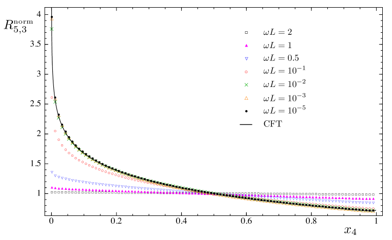
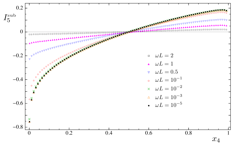
Figure 11: The quantities $R^{\textrm{\tiny{norm}}}_{N=5,n=3}$ (top) and $I^{\textrm{\tiny{sub}}}_{N=5}$ (bottom) in (2.22) computed for the harmonic chain with periodic boundary conditions by employing (5.6) and (5.7). The total length of the chain is $L=5000$. The configuration of the intervals is (5.11) and the fixed one chosen for the normalization is (5.12). The continuos curve in the top panel is the CFT prediction (3.33) and it agrees with the lattice results for $\omega L\ll 1$. We are not able to compute the CFT prediction for the bottom panel.

The two point functions $\langle 0|q_{i}q_{j}|0\rangle$ and $\langle 0|p_{i}p_{j}|0\rangle$ are the elements the correlation matrices $\mathbb{Q}_{rs}=\langle 0|q_{r}q_{s}|0\rangle$ and $\mathbb{P}_{rs}=\langle 0|p_{r}p_{s}|0\rangle$ respectively. For the harmonic chain with periodic boundary conditions that we are considering, they read

$$\langle 0|q_{i}q_{j}|0\rangle = \frac{1}{2L}\sum_{k=0}^{L-1}\frac{1}{M\omega_{k}}\cos\bigg{(}\frac{2\pi k(i-j)}{L}\bigg{)}\,,$$ (5.4)

$$\langle 0|p_{i}p_{j}|0\rangle = \frac{1}{2L}\sum_{k=0}^{L-1}\,M\omega_{k}\cos\bigg{(}\frac{2\pi k(i-j)}{L}\bigg{)}\,.$$ (5.5)

When $i,j=0,\dots,L-1$ run over the whole chain, then $\mathbb{Q}\cdot\mathbb{P}=\mathbb{I}_{L}/4$, which is also known as the generalized uncertainty relation. We remark that the limit $\omega\rightarrow 0$ is not well defined because the $k=0$ term in $\langle 0|q_{i}q_{j}|0\rangle$ diverges; therefore we must keep $\omega>0$. Thus, we set $\omega L\ll 1$ in order to stay in the conformal regime. As explained above, we can work in units $M=K=1$ without loss of generality.
In [57, 58, 61] it has been discussed that, in order to compute the Renyi entropies and the entanglement entropy of a proper subset $A$ (made by $\tilde{\ell}$ sites) of the harmonic chain, first we have to consider the matrices $\mathbb{Q}_{A}$ and $\mathbb{P}_{A}$, obtained by restricting the indices of the correlation matrices $\mathbb{Q}$ and $\mathbb{P}$ to the sites belonging to $A$. Then we compute the eigenvalues of the $\tilde{\ell}\times\tilde{\ell}$ matrix $\mathbb{Q}_{A}\cdot\mathbb{P}_{A}$. Since they are larger than (or equal to) $1/4$, we can denote them by $\{\mu_{1}^{2},\dots,\mu_{\ell}^{2}\}$. Finally, the Renyi entropies are obtained as follows

$$\textrm{Tr}\rho_{A}^{n}=\prod_{a\,=\,1}^{\tilde{\ell}}\left[\bigg{(}\mu_{a}+\frac{1}{2}\bigg{)}^{n}-\bigg{(}\mu_{a}-\frac{1}{2}\bigg{)}^{n}\,\right]^{-1},$$ (5.6)

and the entanglement entropy as

$$S_{A}=\sum_{a\,=\,1}^{\tilde{\ell}}\left[\bigg{(}\mu_{a}+\frac{1}{2}\bigg{)}\log\bigg{(}\mu_{a}+\frac{1}{2}\bigg{)}-\bigg{(}\mu_{a}-\frac{1}{2}\bigg{)}\log\bigg{(}\mu_{a}-\frac{1}{2}\bigg{)}\,\right]\,.$$ (5.7)

This procedure holds also when $A$ is the union of $N$ disjoint intervals $A_{i}$ ($i=1,\dots,N$), which is the situation we are interested in.

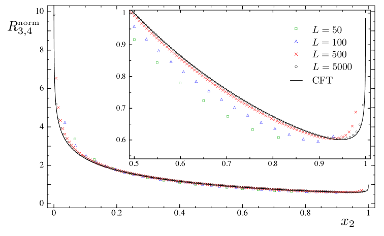
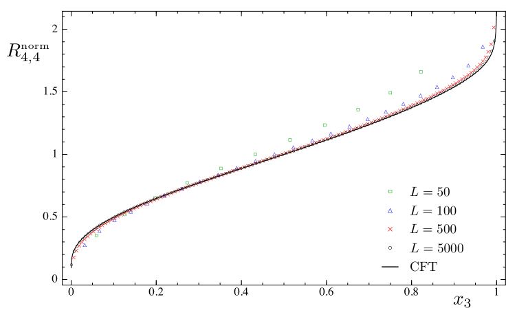
Figure 12: The ratio $R^{\textrm{\tiny{norm}}}_{N,n}$ in (2.22) for the periodic harmonic chain with $\omega L=10^{-3}$ and the configuration of the intervals given by (5.11), normalized through (5.12). The continuos curves are the CFT predictions (3.33). Top: $N=3$ and $n=4$ (in the inset we zoom on part of the region $0.5<x_{2}<1$). Bottom: $N=4$ and $n=4$.

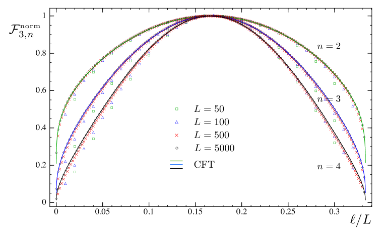
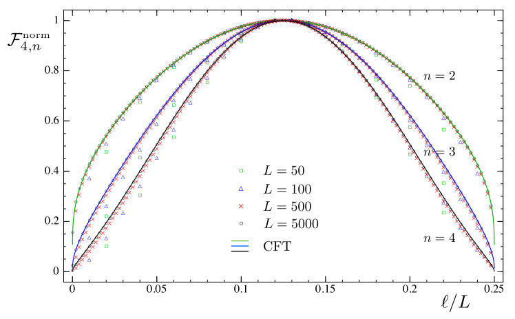
Figure 13: The quantity $\mathcal{F}^{\textrm{\tiny{norm}}}_{N,n}$ computed for the periodic harmonic chain with $\omega L=10^{-3}$ in the configuration of intervals (5.11), normalized through (5.12). The lattice data are obtained by using (2.16), (2.17), (5.6) and (5.7). The continuos curves are given by (3.34). The maximum value on the horizontal axis is $1/N$. We show the cases of $N=3$ (top) and $N=4$ (bottom) with $n=2,3,4$.

Let us denote by $\ell_{i}$ the number of sites included in $A_{i}$ and by $d_{i}$ the number of sites in the separations between $A_{i}$ and $A_{i+1\,\textrm{mod}\,N}$, for $i=1,\dots,N$ (see Fig. 10 for $N=3$). Then, we have that $\tilde{\ell}=\sum_{i=1}^{N}\ell_{i}$ and the following consistency condition about the total length of the chain must be imposed

$$L=\sum_{i\,=\,1}^{N}(\ell_{i}+d_{i})\,.$$ (5.8)

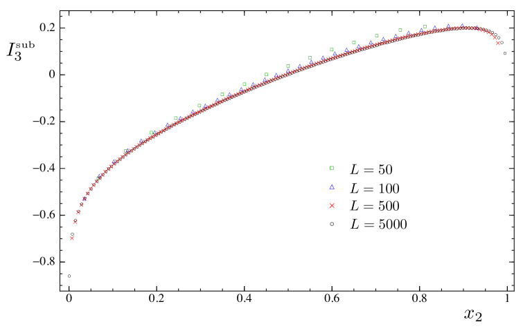
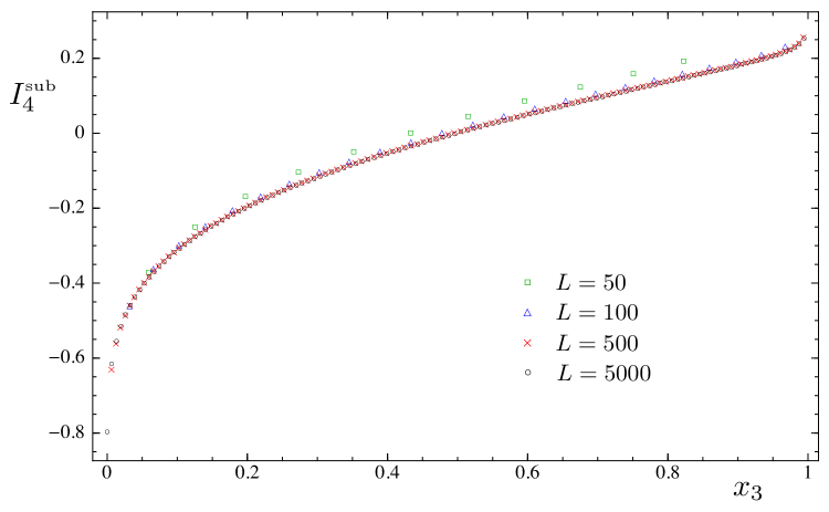
Figure 14: The quantity $I^{\textrm{\tiny{sub}}}_{N}$ (see (2.22)) computed for the periodic harmonic chain with $\omega L=10^{-3}$. The configuration of intervals is given by (5.11) and the fixed one by (5.12). We show $N=3$ (top) and $N=4$ (bottom).

In order to compare the CFT results found in the previous sections with the ones obtained from the harmonic chain in the continuum limit, we have to generalize the CFT formulas to the case of a finite system of total length $L$ with periodic boundary conditions. This can be done by employing the conformal map from the cylinder to the plane, whose net effect is to replace each length $y$ (e.g. $\ell$, $d$, $2\ell+d$, etc.) with the corresponding chord length $(L/\pi)\sin(\pi y/L)$. Thus, for $x_{2j+1}$ with $j=0,\dots,N-2$ we have

$$x_{2j+1}\,=\,\frac{\sin\big{(}\pi\big{[}\sum_{i=1}^{j}(\ell_{i}+d_{i})+\ell_{j+1}\big{]}/L\big{)}\,\sin(\pi\ell_{N}/L)}{\sin\big{(}\pi\sum_{i=1}^{N-1}(\ell_{i}+d_{i})/L\big{)}\,\sin\big{(}\pi\big{[}d_{j+1}+\sum_{i=j+2}^{N-1}(\ell_{i}+d_{i})+\ell_{N}\big{]}/L\big{)}}\,,$$ (5.9)

while for the harmonic ratios $x_{2j}$, where $j=1,\dots,N-2$, we must consider

$$x_{2j}\,=\,\frac{\sin\big{(}\pi\sum_{i=1}^{j}(\ell_{i}+d_{i})/L\big{)}\,\sin(\pi\ell_{N}/L)}{\sin\big{(}\pi\sum_{i=1}^{N-1}(\ell_{i}+d_{i})/L\big{)}\,\sin\big{(}\pi\big{[}\sum_{i=j+2}^{N-1}(\ell_{i}+d_{i})+\ell_{N}\big{]}/L\big{)}}\,.$$ (5.10)

Notice that $d_{N}$, which can be obtained from (5.8), does not occur in these ratios. Moreover, (5.9) and (5.10) depend only on $\ell_{i}/L$ and $d_{i}/L$, with $i=1,\dots,N-1$.

We often consider the configuration where all the intervals have the same length and also the segments separating them have the same size, namely

$$\ell_{1}=\dots=\ell_{N}\equiv\ell\,,\qquad d_{1}=\dots=d_{N}\equiv d\,.$$ (5.11)

This configuration is parameterized by $\ell$, once $d$ has been found in terms of $\ell$ through the condition (5.8). As mentioned in §2, in order to eliminate some parameters, it is useful to normalize the results through a fixed configuration of intervals, as done e.g. in [35, 36, 39]. We choose the following one

$$\textrm{fixed configuration:}\qquad\ell_{1}=\dots=\ell_{N}=d_{1}=\dots=d_{N-1}=\textrm{int}\bigg{(}\frac{L}{2N}\bigg{)}\,,$$ (5.12)

where $\textrm{int}(\dots)$ denotes the integer part of the number within the brackets and $d_{N}$ is obtained from (5.8).
In Figs. 11, 12, 13 and 14 we choose the configuration (5.11) normalized through the fixed one in (5.12). A chain made by $L=5000$ sites gives us a very good approximation of the continuum case. We also made some checks with $L=10000$ in order to be sure that the results do not change significantly. From Fig. 11 we learn that for $\omega L\sim 10^{-3}$ we are already in a regime which is suitable to check the CFT prediction of §3.3, therefore we keep $\omega L=10^{-3}$ for the other plots obtained from the harmonic chain. In order to compare the lattice results from the periodic chain with the CFT expressions (3.31) and (3.32), one needs to adjust $\eta$. We find that this value of $\eta$ depends on the product $\omega L\ll 1$. Nevertheless, as already noticed in §3.3, normalizing the interesting quantities through a fixed configuration as in (2.22), we can ignore this important issue because $\eta$ simplifies (see 3.33 and 3.34)). The Figs. 12 and 13 show that the agreement between the exact results from the harmonic chain and the corresponding CFT predictions is very good. Instead, for the plots in Fig. 14 we do not have a CFT prediction because, ultimately, we are not able to compute $\partial_{n}\widehat{\mathcal{F}}_{N,n}(\boldsymbol{x})$ when $n\rightarrow 1$ for the function defined in (3.31).

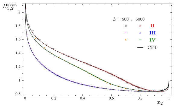
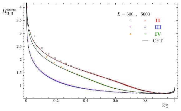
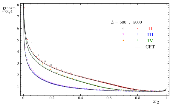
Figure 15: The ratio $R^{\textrm{\tiny{norm}}}_{N,n}$ in (2.22) for the harmonic chain with $\omega L=10^{-3}$. The configurations II, III and IV, which are defined in (5.14), have been normalized through (5.12). The continuos curve is the CFT prediction (3.33). We show $N=3$ and $n=2,3,4$ (top, middle, bottom).

When $N>2$ we have many possibilities to choose the configuration of the intervals. In principle we should test all of them and not only (5.11), as above. For simplicity, we consider two other kinds of configurations defined as follows

$$\rule{0.0pt}{28.45274pt}\begin{array}[]{c|ccccccccc|}&\ell_{1}&d_{1}&\ell_{2}&d_{2}&\ell_{3}&d_{3}&\dots&\ell_{N}&d_{N}\\ \hline\cr\textrm{$\boldsymbol{\lambda}$}&\ell&d&\lambda_{2}\ell&d&\lambda_{3}\ell&d&\dots&\lambda_{N}\ell&d\\ \hline\cr\textrm{$\boldsymbol{\gamma}$}&\ell&d&\gamma_{2}\ell&\gamma_{2}d&\gamma_{3}\ell&\gamma_{3}d&\dots&\gamma_{N}\ell&\gamma_{N}d\\ \hline\cr\end{array}$$ (5.13)

where $\lambda_{i}$ and $\gamma_{i}$ are integer numbers which can be collected as components of the vectors $\boldsymbol{\lambda}$ and $\boldsymbol{\gamma}$. Notice that the configuration (5.11) is obtained either with $\lambda_{i}=1$ or with $\gamma_{i}=1$, for $i=2,\dots,N$. Once the ratios $\lambda_{i}$ or $\gamma_{i}$ have been chosen in (5.13), we are left with $\ell$ and $d$ as free parameters. As above, $d$ can be found as a function of $\ell$ through the condition (5.8) and the maximum value for $\ell$ corresponds to $d=1$. The configurations in (5.13) depend only on the parameter $\ell$; therefore they provide one dimensional curves in the configurations space, which is $2N-3$ dimensional and parameterized by $0<x_{1}<x_{2}<\dots<x_{2N-3}<1$.
When $N=3$, let us consider the configurations (5.13) with the following choices

$$\begin{array}[]{c|lll|}\hline\cr\textrm{ I}&\gamma_{1}=1&\gamma_{2}=1&\gamma_{3}=1\\ \hline\cr\textrm{ II}&\lambda_{1}=1&\lambda_{2}=2&\lambda_{3}=8\\ \hline\cr\textrm{III}&\gamma_{1}=1&\gamma_{2}=3&\gamma_{3}=6\\ \hline\cr\textrm{IV}&\lambda_{1}=1&\lambda_{2}=11&\lambda_{3}=11\\ \hline\cr\end{array}$$ (5.14)

where the first one is (5.11) specialized to the case of three intervals. Plugging these configurations in (5.9) and (5.10) for $N=3$, we can find the corresponding curves within the domain $0<x_{1}<x_{2}<x_{3}<1$, as shown in Fig. 3. These curves can be equivalently parameterized either by $\ell/L$ or by one of the harmonic ratios $x_{i}$. In Fig. 15 we show $R_{3,n}^{\textrm{\tiny{norm}}}$ ($n=2,3,4$), finding a good agreement with the CFT prediction (3.33). In Fig. 16 we plot $I_{3}^{\textrm{\tiny{sub}}}$ for the harmonic chain but, as for Fig. 14, we do not have a CFT formula to compare with for the reason mentioned above.

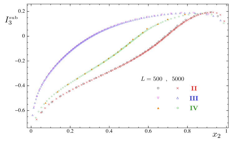
Figure 16: $I^{\textrm{\tiny{sub}}}_{N=3}$ in (2.22) for the periodic harmonic chain with $\omega L=10^{-3}$. The configurations are defined in (5.14) and the fixed one is given by (5.12).

6 The Ising model

The Ising model in transverse field provides a simple scenario where we can compute the Rényi entropies of several disjoint intervals and compare them with the corresponding predictions obtained through the CFT methods. The Hamiltonian is given by

$$H=\sum_{s\,=\,1}^{L}\Big{(}\sigma^{x}_{s}\sigma^{x}_{s+1}+h\sigma^{z}_{s}\Big{)}\,,$$ (6.1)

where $s$ labels the $L$ sites of a 1D lattice $\mathcal{L}$ and the $\sigma_{s}^{x,z}$ are the Pauli matrices acting on the spin at site $s$ and periodic boundary conditions are imposed. The model has two phases, one polarized along $x$ for $\lambda<1$ and another one polarized along $z$ for $\lambda>1$, which are separated by a second order phase transition at $h=1$.
The Ising model in transverse field can be rewritten as a model of free fermions [63]. The map underlying this equivalence has been employed in [64] to compute the Rényi entropies for one block and in [22] for two disjoint blocks, where the generalization to $N$ blocks is also discussed.

Our approach is based on the Matrix Product States (MPS), which is completely general and therefore it can be applied for every one dimensional model. We choose the MPS because they are the simplest tensor networks (see §6.2 for a proper definition). The same calculation can be done through other variational ansatz methods, like the Tree Tensor Networks or the MERA [65, 20, 23]).

6.1 Rényi entropies for the Ising CFT

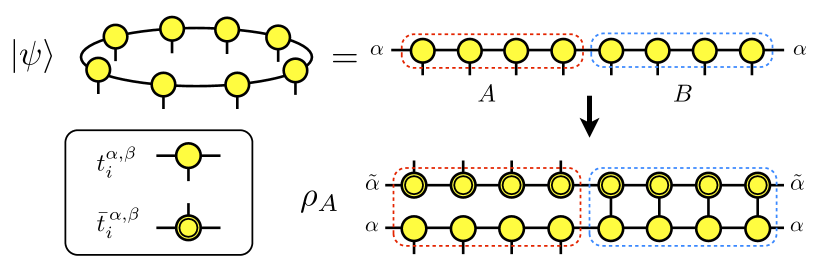
Figure 17: The contraction giving the MPS state $\ket{\psi}$ of a chain with $L=8$ sites and periodic boundary conditions (points labeled by the same greek index are considered as the same point). The individual tensor $t_{i}^{\alpha,\beta}$, which defines the MPS state, and its complex conjugate $\bar{t}_{i}^{\,\alpha,\beta}$ are shown in the box on the left. Considering the bipartition of the chain with $A$ made by 4 contiguous sites, we show the tensor network contraction occurring in the computation of the reduced density matrix $\rho_{A}$.

The continuum limit of the quantum critical point $h=1$ corresponds to a free massless Majorana fermion, which is a CFT with $c=1/2$.

Identifying $\phi$ with $-\,\phi$ in (3.1), the target space becomes $S^{1}/\mathbb{Z}_{2}$ and the compactification radius (orbifold radius) parameterizes the critical line of the Ashkin-Teller model, which can be seen as two Ising models coupled through a four fermion interaction. When the interaction vanishes, the partition function of the Ashkin-Teller model reduces to the square of the partition function of the Ising model.
This set of $c=1$ conformal field theories has been studied in [9, 10, 11, 14] in the case of a worldsheet given by a generic Riemann surface and the relations found within this context allow us to write ${\rm Tr}\rho_{A}^{n}$ for the Ising model in terms of Riemann theta functions with characteristic (3.35). The peculiar feature of the Ising model with respect to the other points of the Ashkin-Teller line is that we just need the period matrix $\tau$ to find the partition function on the corresponding Riemann surface.

In our case, the Riemann surface is given by (3.3) and its period matrix has been computed in §3.1. Thus, ${\rm Tr}\rho_{A}^{n}$ for the Ising model is given by (1.5) with $c=1/2$ and

$$\mathcal{F}^{\textrm{\tiny Ising}}_{N,n}(\boldsymbol{x})=\frac{\sum_{\boldsymbol{e}}|\Theta[\boldsymbol{e}](\boldsymbol{0}|\tau)|}{2^{g}\,|\Theta(\boldsymbol{0}|\tau)|}\,,$$ (6.2)

where the period matrix $\tau$ has been discussed in §3.1. As already remarked in §3.4, the sum over the characteristics in the numerator of (6.2) contains only the even ones. We checked numerically that $\mathcal{F}^{\textrm{\tiny Ising}}_{N,n}(\boldsymbol{0})=1$. Moreover, by employing the results of §4 and of Appendix C, one finds that, specializing (6.2) to $N=2$, the expression for $\mathcal{F}^{\textrm{\tiny Ising}}_{2,n}(x)$ found in [6] is recovered. In Appendix C we also discuss the invariance of (6.2) under a cyclic transformations or an inversion in the ordering of the sheets and under the exchange $A\leftrightarrow B$.

6.2 Matrix product states: notation and examples

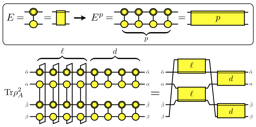
Figure 18: The computation of $\textrm{Tr}\rho_{A}^{2}$ for the bipartition of Fig. 17, where $\ell=d=4$. The MPS transfer matrix $E$ and its $p$-th power are shown in the box as yellow rectangles. The pattern for the contractions of the indices is on the right.

A pure state $\ket{\Psi}\in\mathbb{V}^{\otimes L}$ defined on the lattice $\mathcal{L}$ can be expanded in the local basis of $\mathbb{V}_{s}$ given by $\{\ket{1_{s}},\ket{2_{s}},\cdots,\ket{\delta_{s}}\}$ as follows

$$|\Psi\rangle\,=\sum_{i_{1}=1}^{\delta}~{}\sum_{i_{2}=1}^{\delta}\cdots\sum_{i_{L}=1}^{\delta}T_{i_{1}i_{2}\cdots i_{L}}\ket{i_{1}}\ket{i_{2}}\cdots\ket{i_{L}}\,.$$ (6.3)

This means that $\ket{\Psi}$ is encoded in a tensor $T$ with $\delta^{L}$ complex components $T_{i_{1}i_{2}\cdots i_{L}}\in\mathbb{C}$. We refer to the index $1\leqslant i_{s}\leqslant\delta$, labelling a local basis for site $s$, as the physical index.

The tensor network approach (see e.g. the review [32]) is a powerful way to rewrite the exponentially large tensor $T$ in (6.3) as a combination of smaller tensors. In order to simplify the notation, drawings are employed to represent the various quantities occurring in the computation. Tensors are represented by geometric shapes (circles or rectangles) having as many legs as the number of indices of the tensor. The complex conjugate of a tensor is denoted through the same geometric object delimited by a double line. A line shared by two tensors represents the contraction over the pair of indices joined by it.

The Matrix Product States (MPS) are tensor networks that naturally arise in the context of the Density Matrix Renormalization Group [66, 67, 68]. They are build through a set of tensors $t_{i}^{\alpha,\beta}$ (one for each lattice site) with three indices (see the box in Fig. 17): $i$ is the physical index mentioned above, while $\alpha$ and $\beta$ are auxiliary indices. The tensors are contracted following the pattern shown in Fig. 17, where the translational invariance of the state is imposed by employing the same elementary tensor for each site. The state in Fig. 17 has $L=8$ and it is given by

$$|\Psi\rangle=\sum_{i_{1},\dots,i_{8}=1}^{\delta}\;\sum_{\alpha_{1},\dots,\alpha_{8}=1}^{\chi}t_{i_{1}}^{\alpha_{1}\alpha_{2}}\,t_{i_{2}}^{\alpha_{2}\alpha_{3}}\cdots\,t_{i_{8}}^{\alpha_{8}\alpha_{1}}\ket{i_{1}}\ket{i_{2}}\cdots\ket{i_{8}}\,,$$ (6.4)

where $\chi$ is the rank of the auxiliary indices, which is called bond dimension in this context. Since we are using the same tensor for each site, the state is completely determined by the components of the tensor $t_{i}^{\alpha\beta}$, which are $\delta\chi^{2}$ free parameters. In the MPS approach, the expectation value of local observables can be computed by performing $\mathcal{O}(\delta\chi^{3})$ operations. The components $t_{i}^{\alpha\beta}$ of the tensor are obtained numerically by minimizing $\langle\Psi|H|\Psi\rangle$ for the Hamiltonian (6.1).

Figure 19: The two point correlation function $C(r)_{{\cal O}_{1},{\cal O}_{2}}$ of the local operators ${\cal O}_{1}$ and ${\cal O}_{2}$. The corresponding generalized transfer matrices $E({\cal O}_{1})$ and $E({\cal O}_{2})$, depicted in the box, must be contracted with the proper powers of $E$.

The bond dimension $\chi$ controls the accuracy of the results. Increasing $\chi$, one can describe an arbitrary state of the Hilbert space [69]. In practice, a finite bond dimension which is independent of $L$ allows to describe accurately ground states of gapped local Hamiltonians [70]. For gapless Hamiltonians described by a CFT, the bond dimension has to increase polynomially with the system size [71], namely $\chi=L^{1/\kappa}$, where $\kappa$ is an universal exponent [72] which depends only on the central charge $c$ as follows: $\kappa=6/[c(\sqrt{12/c}+1)]$ [73, 74]. Since the Ising model has $c=1/2$, we have $\kappa\simeq 2$.

In principle, the MPS representation of the ground state allows us to compute several observables. In practice, different computations require a different computational effort. For instance, considering the bipartition shown in Fig. 17, where $L=8$ and $\ell=4$, the reduced density matrix $\rho_{A}$ in a MPS representation has at most rank $\chi^{2}$ [32, 75], independently on the size of the block. This implies that it can be computed exactly by performing at most $\mathcal{O}(\delta^{3}\chi^{6})$ operations.

The case of $N$ disjoint blocks is more challenging. Indeed, the corresponding reduced density matrices in the MPS representation can have rank up to $\chi^{2N}$, which means that these computations are exponentially hard in $N$. Some of these computation can be done by projecting the reduced density matrices on their minimal rank [20, 23]. Here we describe an alternative approach, which is based on the direct computation of the Rényi entropies.

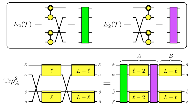
Figure 20: The computation of $\textrm{Tr}\rho_{A}^{2}$ of Fig. 18 as the two point correlation function (see Fig. 19) of twist fields in the MPS formalism, i.e. through (6.7). They are operators acting on the auxiliary degrees of freedom and this allows us to define the generalized transfer matrices $E_{2}({\cal T})$ and $E_{2}(\bar{{\cal T}})$, which must be contracted with the proper powers of $E_{2}$.

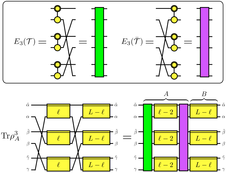
Figure 21: The computation of $\textrm{Tr}\rho_{A}^{3}$ of Fig. 18 as the two point correlation function (see Fig. 19) of twist fields (6.7). In this case the twist fields act on the tensor product of three pairs of virtual indices. The generalized transfer matrices $E_{3}({\cal T})$ and $E_{3}(\bar{{\cal T}})$ are contracted with the proper powers of $E_{3}=E\otimes E\otimes E$.

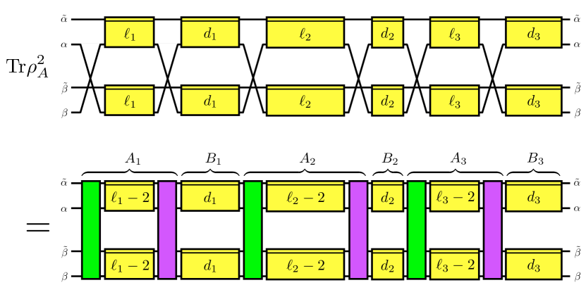
Figure 22: The computation of $\textrm{Tr}\rho_{A}^{n}$ through (6.8) in the case of $N=3$ and $n=2$ as the six point function of twist fields.

6.3 Rényi entropies from MPS: correlation functions of twist fields

In the computation of $\textrm{Tr}\rho_{A}^{n}$, which gives the Rényi entropies through (1.2), we need the powers of the MPS transfer matrix $E^{(\alpha,\tilde{\alpha}),(\beta,\tilde{\beta})}\equiv\sum_{i}{t_{i}^{\alpha,\beta}\bar{t}_{i}^{\,\tilde{\alpha},\tilde{\beta}}}$. Being a mixed tensor involving both $t$ and $\bar{t}$, we represent $E$ as the yellow rectangle in the box of Fig. 18, where the double line on one side keeps track of the position of $\bar{t}$. Then, we can straightforwardly construct the $p$-th power $E^{p}$, which is the key ingredient to obtain $\textrm{Tr}\rho_{A}^{n}$ for a bipartition of the chain. Indeed, when $A$ is made by a block of length $\ell$, it is computed in terms of $E^{\ell}$ and $E^{d}$, where $d=L-\ell$. In Fig. 18 we represent the computation of $\textrm{Tr}\rho_{A}^{2}$ for the bipartition of Fig. 17.

Simple manipulations allow us to write the above expression for $\textrm{Tr}\rho_{A}^{n}$ as the two point function of twist fields. In order to see this, let us first consider the two point correlation function $C_{{\cal O}_{1},{\cal O}_{2}}(r)\equiv\langle\psi|{\cal O}_{1}(x){\cal O}_{2}(x+r)|\psi\rangle$ of local operators ${\cal O}_{1}$ and ${\cal O}_{2}$. For this computation we introduce the generalized transfer matrix for a generic local operator $\mathcal{O}$ as

$$E(\mathcal{O})^{(\alpha,\alpha^{\prime}),(\beta,\beta^{\prime})}\equiv\sum_{i,j}t_{i}^{\alpha,\beta}\bar{t}_{j}^{\,\tilde{\alpha},\tilde{\beta}}\mathcal{O}^{i,j}\,,$$ (6.5)

whose graphical representation is shown in the box of Fig. 19. Given (6.5), the two point correlation function becomes the following trace of the product of transfer matrices

$$C_{{\cal O}_{1},{\cal O}_{2}}(r)=\textrm{Tr}\big{(}E({\cal O}_{1})E^{r-2}E({\cal O}_{2})E^{L-r}\big{)}\,,$$ (6.6)

which is depicted in Fig. 19, where different colors correspond to different operators.

In a similar way, we can write $\textrm{Tr}\rho_{A}^{n}$ for the bipartition of Fig. 17 as the two point correlation function of twist fields. This is done by introducing other generalized transfer matrices, namely the tensor product $E_{n}=E\otimes\dots\otimes E$ of $n$ transfer matrices and the transfer matrices $E_{n}({\cal T})$ and $E_{n}(\bar{{\cal T}})$ associated to the twist fields (see the box in Fig. 20 for $n=2$ and in Fig. 21 for $n=3$). Given these matrices, $\textrm{Tr}\rho_{A}^{n}$ reads

$$\textrm{Tr}\rho_{A}^{n}=\textrm{Tr}\big{(}E_{n}({\cal T})E_{n}^{\ell-2}E_{n}(\bar{{\cal T}})E_{n}^{L-\ell}\big{)}\,.$$ (6.7)

Notice that (6.7) has the structure of the two point function given in 6.6, but it is not exactly the same. Indeed, since the twist fields are operators acting on the virtual bonds rather than on the physical bonds, they are not local operators on the original spin chain. In Figs. 20 and 21 we show (6.7) for $n=2$ and $n=3$ respectively.

It is straightforward to generalize this construction to the case of $N$ disjoint blocks (see Fig. 10 for the notation). In this case $A=\cup_{i=1}^{N}A_{i}$ and the generalization of (6.7) to $N\geqslant 2$ reads

$$\textrm{Tr}\rho_{A}^{n}=\textrm{Tr}\big{(}E_{n}({\cal T})E_{n}^{\ell_{1}-2}E_{n}(\bar{{\cal T}})E_{n}^{d_{1}}\cdots E_{n}({\cal T})E_{n}^{\ell_{N}-2}E_{n}(\bar{{\cal T}})E_{n}^{d_{N}}\big{)}\,,$$ (6.8)

where the dots replace the sequence of terms $E_{n}({\cal T})E_{n}^{\ell_{j}-2}E_{n}(\bar{{\cal T}})E_{n}^{d_{j}}$, ordered according to the increasing value of interval index $j=2,\dots,N-1$. In Fig. 22, the MPS computation (6.8) for $N=3$ and $n=2$ is depicted. It is important to remark that in (6.8) the computational cost is $O(N\delta\chi^{4n+1})$, i.e. exponential in $n$ and linear in $N$. Thus, for the simplest cases of $n=2$ and $n=3$ the cost is $\chi^{9}$ and $\chi^{13}$ respectively. Because of this, in the remaining part of this section we present numerical results obtained through the exact formula (6.8) with $n=2$ only, for configurations made by either $N=3$ or $N=4$ disjoint blocks.

The method that we just discussed is very general and, in principle, it can be applied for many lattice models. Nevertheless, the feasibility of the computation strongly depends on the value of the bond dimension $\chi$, which depends on the central charge $c$ as mentioned above. Thus, having $c=1/2$, the Ising model is the easiest model that we can deal with. A model with $c=1$ would lead to a very high computational cost already for the Rényi entropy with $n=2$ and this would be a very challenging computation, given the numerical resources at our disposal.

As for the approximate calculations of the Rényi entropies, a very different scenario arises. In particular, Monte Carlo techniques [18, 76, 77, 78] look very promising because they allow to obtain an approximate result for $\textrm{Tr}\rho_{A}^{n}$ by sampling over the physical indices. Each configuration can be computed with $n\chi^{3}$ operations, but the number of configurations which are necessary to extract a reliable estimation of the Rényi entropies in terms of $\chi$ and $n$ is still not understood.

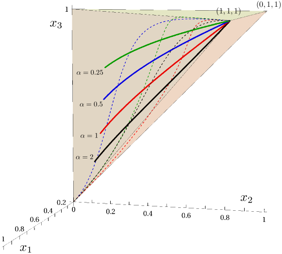
Figure 23: The domain $0<x_{1}<x_{2}<x_{3}<1$ for $N=3$, as in Fig. 3. The thick lines represent the configurations (6.9) for some choices of $\alpha$. The dashed thin curves are the configurations shown in Fig. 3, with the same colors.

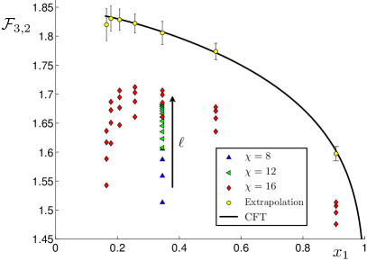
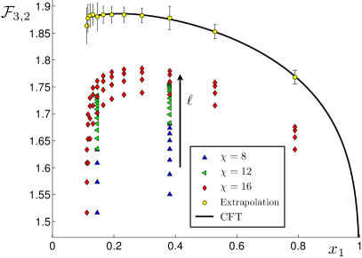
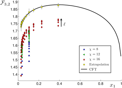
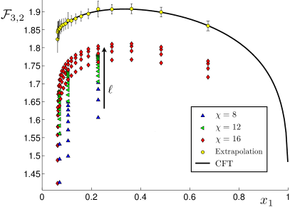
Figure 24: The results for $\mathcal{F}_{3,2}$ computed through MPS. The configurations are (6.9) with (from the top left panel, in clockwise direction) $\alpha=0.25$, $\alpha=0.5$, $\alpha=1$ and $\alpha=2$. For a fixed $\boldsymbol{x}$, the length $\ell$ of the blocks increases along the black arrow. The extrapolated points are obtained as explained in §6.4.

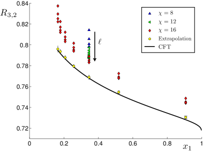
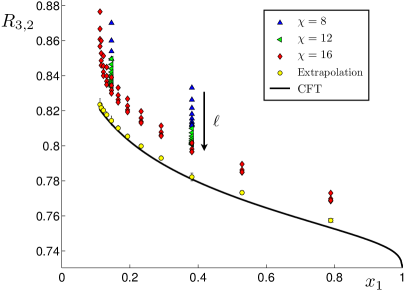
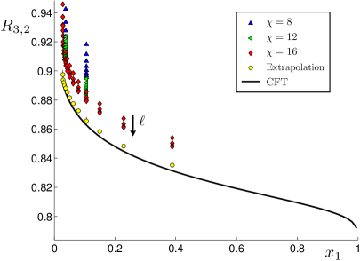
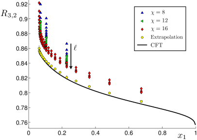
Figure 25: The results for $R_{3,2}$ computed through MPS. The configurations are (6.9) with (from the top left panel, in clockwise direction) $\alpha=0.25$, $\alpha=0.5$, $\alpha=1$ and $\alpha=2$. For a fixed $\boldsymbol{x}$, the length $\ell$ of the blocks increases along the black arrow. The extrapolated points are obtained as explained in §6.4.

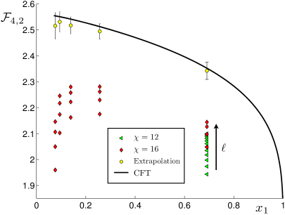
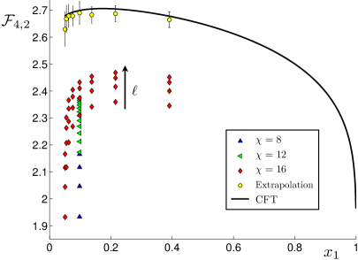
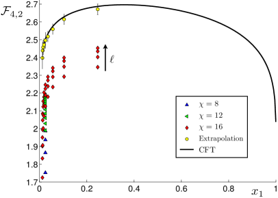
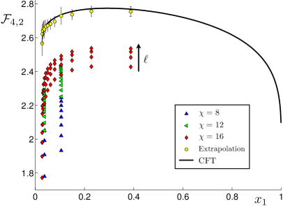
Figure 26: The results for $\mathcal{F}_{4,2}$ computed through MPS. The configurations are (6.9) with (from the top left panel, in clockwise direction) $\alpha=0.25$, $\alpha=0.5$, $\alpha=1$ and $\alpha=2$. For a fixed $\boldsymbol{x}$, the length $\ell$ of the blocks increases along the black arrow. The extrapolated points are obtained as explained in §6.4.

6.4 Numerical results for $n=2$

Let us discuss the numerical results obtained through the method discussed in §6.3 about ${\rm Tr}\rho^{2}_{A}$ for the Ising model with periodic boundary conditions. The length $L$ of the chains varies within the range $30\leqslant L\leqslant 500$. The MPS matrices have been computed by employing the variational algorithm described in [79] (see also the ones in [80, 81]). Moreover, from Fig. 2 of [74] one observes that, in order to find accurate results for the Ising model in the range of total lengths given above, we need $8\leqslant\chi\leqslant 16$.

As for the configurations of the $N$ disjoint blocks of sites, denoting by $\ell_{i}$ the number of sites for the block $A_{i}$ and by $d_{i}$ the number of sites separating $A_{i}$ and $A_{i+1\,\textrm{mod}\,N}$ with $i=1,\dots,N$ as in §5 (see Fig. 10 for the case $N=3$), we find it convenient to choose the following ones

$$\rule{0.0pt}{19.91684pt}\begin{array}[]{|ccccccccc|}\ell_{1}&d_{1}&\ell_{2}&d_{2}&\ell_{3}&d_{3}&\dots&\ell_{N}&d_{N}\\ \hline\cr\ell&d&\ell&d&\ell&d&\dots&\ell&d_{N}\\ \hline\cr\end{array}\qquad\begin{array}[]{c}\\ d=\alpha\ell\,,\end{array}$$ (6.9)

where $d_{N}=L-[N+\alpha(N-1)]\ell$ is fixed by the consistency condition (5.8) on the total length of the chain. Thus, each configuration is characterized by the coefficient $\alpha$ and the free parameter is $\ell$. In the comparison with the CFT expressions discussed in §2 and §6.1, we have taken the finiteness of the system into account through (5.9) and (5.10), as already done in §5 for the harmonic chain. Like for (5.13) with the vectors $\boldsymbol{\lambda}$ and $\boldsymbol{\gamma}$ fixed, also for the configurations (6.9) with $\alpha$ fixed the harmonic ratios $x_{i}$ depend only on $\ell/L$, providing one dimensional curves within the $2N-3$ dimensional configuration space $0<x_{1}<x_{2}<\dots<x_{2N-3}<1$. Nevertheless, notice that in this case the harmonic ratios have a strictly positive lower bound, which can be computed by taking the limit $\ell/L\rightarrow 0$ in the expressions of $x_{i}$ obtained by specializing (5.9) and (5.10) to (6.9). For instance, when $N=3$ we have $x_{1}=[\sin(\pi\ell/L)/\sin(2\pi(1+\alpha)\ell/L)]^{2}$, whose smallest value reads $1/[2(1+\alpha)]^{2}$. Always for $N=3$, in Fig. 23 we show the curves corresponding to the configurations (6.9) for the numerical values of $\alpha$ considered in the remaining figures. Each curve can be equivalently parameterized by one of the harmonic ratios and in this section we choose $x_{1}$ as the independent variable.

Given the configurations (6.9), for any fixed $\alpha$ different values of $\ell$ and $L$ having the same $\ell/L$ provide the same $\boldsymbol{x}$, i.e. the same point in the configurations space. Aligning the numerical data corresponding to the same $\boldsymbol{x}$, one observes that, as $\ell$ increases, they approach the CFT prediction. Nevertheless, the discrepancy is quite large because the chains at our disposal are not long enough. Thus, unlike the case of the harmonic chain discussed in §5, for the Ising model the plots of the data do not immediately confirm the CFT expressions.

During the last few years many papers have studied the corrections to the leading scaling behavior of the Rényi entropies [82, 83, 84, 20, 22, 85, 86, 23, 39, 87]. When $A$ is a single block made by $\ell$ contiguous lattice sites within a periodic chain of length $L$, the first deviation of ${\rm Tr}\rho_{A}^{n}$ from the corresponding value obtained through the CFT expression is proportional to $\ell^{-2\Delta/n}$, for some $\Delta<2$. From the field theoretical point of view, this unusual scaling can be understood by assuming that the criticality is locally broken at the branch points and this allows the occurrence of relevant operators with scaling dimension $\Delta<2$ at those points [84]. For the Ising model the relevant operators must be also parity even and this means that the first correction is proportional to $\ell^{-2/n}$. Instead, when $A$ is made by two disjoint blocks, it has been numerically observed that the leading correction for the Ising model is proportional to $\ell^{-1/n}$ [20, 22], which agrees with $\ell^{-2\Delta/n}$ with $\Delta=1/2$. This could be the contribution of the Majorana fermion introduced by the Jordan-Wigner string between the two blocks [22].

In the following we consider the case of $A$ made by three and four disjoint blocks, focusing on $\mathcal{F}_{3,2}$ and $R_{3,2}$ for $N=3$ and on $\mathcal{F}_{4,2}$ for $N=4$. We studied the configurations (6.9) with $\alpha=p$ and $\alpha=1/p$, where for the integer $p$ we took $1\leqslant p\leqslant 8$. Here we show the plots only for $\alpha\in\{0.25,0.5,1,2\}$ because the ones for the remaining values of $\alpha$ are very similar. The results for $N=3$ are reported in Figs. 24 and 25, while the ones for $N=4$ are given in Fig. 26. Different colored shapes denote numerical data which have been obtained from ground states with different bound dimensions. Moreover, for fixed values of $\boldsymbol{x}$ and $\chi$, the black arrow indicates the direction along which $\ell$ increases. For a given $\chi$, the maximum value $L_{\textrm{max}}$ of the total size of the chain has been determined according to Fig. 2 of [74]. In particular, for $\chi=8$, $\chi=12$ and $\chi=16$ we used respectively $L_{\textrm{max}}=100$, $L_{\textrm{max}}=320$ and $L_{\textrm{max}}=500$.

Notice that larger values of $\chi$ and $\ell$ better approximate the points obtained through the CFT formulas, as expected. Nevertheless, since the discrepancy between our best numerical value and the one predicted by the CFT is quite large, a finite size scaling analysis is necessary, as discussed above. For almost every value of $\boldsymbol{x}$ that we are considering, taking the effects of the first correction into account is enough to find reasonable agreement with the CFT predictions. According to the analysis discussed in Appendix D.1, we find that the first correction is proportional to $\ell^{-\Delta_{\textrm{num}}}$, where $\Delta_{\textrm{num}}=0.45(5)$ for both $\mathcal{F}_{3,2}$ and $\mathcal{F}_{4,2}$, and $\Delta_{\textrm{num}}=0.51(4)$ for $R_{3,2}$. We remark that these exponents have been found just from the numerical data, without assuming the CFT formulas. The result is compatible with $\Delta=1/2$ found for two disjoint blocks [20, 22]. Thus, this result seems to be independent of the number of intervals.

Once the exponents have been determined, we can compare the numerical results with the CFT predictions. This means that, for $N=3$ and $N=4$, we consider

$$\mathcal{F}^{\textrm{\tiny\,lat}}_{N,2}(\boldsymbol{x})=\mathcal{F}^{\textrm{\tiny\,ext}}_{N,2}(\boldsymbol{x})+\frac{f_{N}(\boldsymbol{x})}{\ell^{\Delta_{\textrm{num}}}}\,,\qquad R^{\textrm{\tiny\,lat}}_{3,2}(\boldsymbol{x})=R^{\textrm{\tiny\,ext}}_{3,2}(\boldsymbol{x})+\frac{r(\boldsymbol{x})}{\ell^{\Delta_{\textrm{num}}}}\,,$$ (6.10)

where $\Delta_{\textrm{num}}$ are the exponents given above. For any fixed $\boldsymbol{x}$, we have two parameters to fit: the coefficient of $\ell^{-\Delta_{\textrm{num}}}$ and the extrapolated value. The latter one must be compared with the corresponding value obtained through the CFT formula. Since we have to find only two parameters through this fitting procedure, we can carry out this analysis for all the $\boldsymbol{x}$’s at our disposal, also when few numerical points occur. Because of the uncertainty on $\Delta_{\textrm{num}}$, for any fixed $\boldsymbol{x}$ we perform the extrapolation for both the maximum and the minimum value of $\Delta_{\textrm{num}}$. This provides the error bars indicated in Figs. 24, 25 and 26, where the yellow circles denote the mean values.

In Appendix D.2 we consider more than one correction, keeping the same exponents employed for the case $N=2$ [22, 23, 39]. Unfortunately, this analysis can be performed only for those few values of $\boldsymbol{x}$ at fixed $\alpha$ which have many numerical points (see Figs. 32 and 33). We typically find that the second correction improves the agreement with the corresponding CFT prediction, as expected, while the third one does not, telling us that, probably, given our numerical data, we cannot catch the third correction.

In Appendix D.3 we briefly consider the effects due to the finiteness of the bond dimension in our MPS computations. They occur because finite $\chi$ leads to a finite correlation length $\xi_{\chi}$ and, whenever it is smaller than the relevant length scales a deviation from the expected power law behavior of the correction is observed [88, 71, 72, 74].

7 Conclusions

In this paper we have computed the Rényi entropies of $N$ disjoint intervals for the simple conformal field theories given by the free compactified boson and the Ising model.

For the free boson compactified on a circle of radius $R$, we find that ${\rm Tr}\rho_{A}^{n}$ for $A=\cup_{i=1}^{N}A_{i}$ with $N\geqslant 2$ is given by (1.5) with $c=1$ and

$$\mathcal{F}_{N,n}(\boldsymbol{x})=\frac{\Theta(\boldsymbol{0}|T_{\eta})}{|\Theta(\boldsymbol{0}|\tau)|^{2}}\,,\qquad T_{\eta}=\begin{pmatrix}\,{\rm i}\,\eta\,\mathcal{I}&\mathcal{R}\\ \mathcal{R}&{\rm i}\,\mathcal{I}/\eta\,\end{pmatrix},$$ (7.1)

where $\eta\propto R^{2}$, the function $\Theta$ is the Riemann theta function (3.22) and $\tau=\mathcal{R}+{\rm i}\,\mathcal{I}$ is the period matrix of the Riemann surface $\mathscr{R}_{N,n}$ defined by (3.3), which has genus $g=(N-1)(n-1)$ (see e.g. Fig. 5, where $N=3$ and $n=4$). As for the Ising model, we find that ${\rm Tr}\rho_{A}^{n}$ is (1.5) with $c=1/2$ and

$$\mathcal{F}^{\textrm{\tiny Ising}}_{N,n}(\boldsymbol{x})=\frac{\sum_{\boldsymbol{e}}|\Theta[\boldsymbol{e}](\boldsymbol{0}|\tau)|}{2^{g}\,|\Theta(\boldsymbol{0}|\tau)|}\,,$$ (7.2)

being $\boldsymbol{e}$ the characteristics of the Riemann theta function, defined through (3.35). The period matrix of $\mathscr{R}_{N,n}$ [30] has been computed for two different canonical homology bases and, given the relation between them, one can employ either (3.20) or (4.11) in the expressions (7.1) and (7.2). The peculiar feature of the free compactified boson and of the Ising model is that, in order to write the Rényi entropies, we just need the period matrix of $\mathscr{R}_{N,n}$.

We have checked (7.1) in the decompactification regime against exact results for the harmonic chain with periodic boundary conditions, finding excellent agreement. As for the Ising model, we have performed an accurate finite size scaling analysis using Matrix Product States. In particular we have identified the twist fields within this formalism, showing that the Rényi entropies can be computed as correlation functions of twist fields also in this case. Whenever a reliable finite size scaling analysis can be performed, the numerical results confirm (7.2). The results of [5, 6] for two disjoint intervals are recovered as special cases of (7.1) and (7.2).

We have not been able to analytically continue (7.1) and (7.2), in order to find the entanglement entropy. We recall that this is still an open problem in the simplest case of two intervals for the free boson at finite $\eta$ and for the Ising model. For the boson on the infinite line, we have shown numerical predictions for the tripartite information and for the corresponding quantities in the case of $N>3$.

It is very important to provide further numerical checks of our CFT predictions, in particular for the free boson at finite compactification radius, as done in [22, 23] for two intervals. Let us mention that it would be extremely interesting to extend the field theoretical computation of the Rényi entropies and of the entanglement entropy of disjoint regions to the massive case [89] and to higher dimensions [90].

Appendices

Appendix A On the $\boldsymbol{x}$ dependence of $R_{N,n}$

In this appendix we give some details about the ratio $R_{N,n}$ defined in (2.10) in the case of two dimensional conformal field theories, when $A=\cup_{i=1}^{N}A_{i}$.

In the simplest case of $N=2$ there is only one harmonic ratio $x\in(0,1)$ defined through (2.6). The two quantities (2.16) and (2.10) coincide and one easily finds that

$$R_{2,n}(x)=\tilde{R}_{2,n}(x)=\frac{\mathcal{F}_{2,n}(x)}{(1-x)^{2\Delta_{n}}}\,.$$ (A.1)

When $N>2$, first we remark that the non universal constant $c_{n}$ cancels in the ratio (2.10) and this is found by employing the same combinatorial identity occurring for the cutoff independence of $R_{N,n}$, discussed in the section 2. Moreover in (2.10) all the factors $P_{p}(\sigma_{N,p})$ cancel, namely

$$\prod_{p\,=\,1}^{N}\,\prod_{\sigma_{N,p}}\big{[}P_{p}(\sigma_{N,p})\big{]}^{(-1)^{N-p}}=1\,.$$ (A.2)

This result can be obtained by writing the l.h.s. as the product of two factors

$$\prod_{p\,=\,1}^{N}\,\prod_{\sigma_{N,p}}\,\prod_{i\,\in\,\sigma_{N,p}}\frac{1}{(v_{i}-u_{i})^{(-1)^{N-p}}}\,,\qquad\prod_{p\,=\,1}^{N}\,\prod_{\sigma_{N,p}}\;\prod_{\begin{subarray}{c}i,j\in\sigma_{N,p}\\ i\,<\,j\end{subarray}}\bigg{[}\,\frac{(u_{j}-u_{i})(v_{j}-v_{i})}{(v_{j}-u_{i})(v_{i}-u_{j})}\,\bigg{]}^{(-1)^{N-p}}.$$ (A.3)

Then, collecting the different factors, they become respectively

$$\prod_{p=1}^{N}\,\prod_{i\,=\,1}^{N}\frac{1}{(v_{i}-u_{i})^{\xi_{p}(-1)^{N-p}}}\,,\qquad\hskip 25.6073pt\prod_{p\,=\,1}^{N}\;\prod_{\begin{subarray}{c}i,j=1\\ i\,<\,j\end{subarray}}^{N}\bigg{[}\,\frac{(u_{j}-u_{i})(v_{j}-v_{i})}{(v_{j}-u_{i})(v_{i}-u_{j})}\,\bigg{]}^{\zeta_{p}(-1)^{N-p}},$$ (A.4)

where we denoted by $\xi_{p}=\binom{N-1}{p-1}$ the number of choices $\sigma_{N,p}$ containing the $i$-th interval and by $\zeta_{p}=\binom{N-2}{p-2}$ the number of $\sigma_{N,p}$’s containing both the $i$-th and $j$-th interval. By employing the combinatorial identities $\sum_{p=1}^{N}(-1)^{N-p}\xi_{p}=0$ and $\sum_{p=2}^{N}(-1)^{N-p}\zeta_{p}=0$ respectively, it is straightforward to conclude that the products in (A.3) are separately equal to 1. Thus, we have that $R_{N,n}(\boldsymbol{x})$ is given by (2.21).

As for the dependence on $\boldsymbol{x}$ of (2.21), let us consider the choice $\sigma_{N,p}=\{i_{1},\dots,i_{p}\}$ of $p$ intervals with $1<p\leqslant N$, corresponding to the subregion $A_{i_{1}}\cup\dots\cup A_{i_{p}}$ included in $A$. Then one introduces the map

$$w_{\sigma_{N,p}}(z)=\frac{(u_{i_{1}}-z)(u_{i_{p}}-v_{i_{p}})}{(u_{i_{1}}-u_{i_{p}})(z-v_{i_{p}})}\,,$$ (A.5)

which is constructed to send $u_{i_{1}}\rightarrow 0$, $u_{i_{p}}\rightarrow 1$ and $v_{i_{p}}\rightarrow\infty$. When $p=N$, the map (A.5) becomes (2.6). The function $\mathcal{F}_{p,n}(\boldsymbol{x}^{\sigma_{N,p}})$ depends on the $2p-3$ harmonic ratios obtained as the images of the remaining endpoints through the map (A.5), namely

$$\mathcal{F}_{p,n}(\boldsymbol{x}^{\sigma_{N,p}})=\mathcal{F}_{p,n}(w_{\sigma_{N,p}}(v_{i_{1}}),\dots,w_{\sigma_{N,p}}(v_{i_{p-1}}))\,.$$ (A.6)

Since the ratios $w_{\sigma_{N,s}}(u_{i_{r}})$ and $w_{\sigma_{N,s}}(v_{i_{r}})$ can be expressed in terms of the harmonic ratios in $\boldsymbol{x}$ by applying (2.6), we have that $R_{N,n}=R_{N,n}(\boldsymbol{x})$. The final expression can be checked by considering the limits $x_{j}\rightarrow x_{j\pm 1}$, whose result can be understood by using that the first operator occurring in the OPE of a twist field $\mathcal{T}_{n}$ with $\bar{\mathcal{T}}_{n}$ is the identity.

We find it useful to write explicitly $R_{N,n}(\boldsymbol{x})$ in the simplest cases. For $N=3$

$$R_{3,n}(\boldsymbol{x})=\frac{\mathcal{F}_{3,n}(x_{1},x_{2},x_{3})}{\mathcal{F}_{2,n}(\frac{x_{1}(x_{3}-x_{2})}{x_{2}(x_{3}-x_{1})})\,\mathcal{F}_{2,n}(x_{1})\,\mathcal{F}_{2,n}(\frac{x_{3}-x_{2}}{1-x_{2}})}\,.$$ (A.7)

From this expression (we recall that $\mathcal{F}_{2,n}(0)=\mathcal{F}_{2,n}(1)=1$), we can check that $R_{3,n}\rightarrow 1$ when $x_{3}\rightarrow x_{2}$ (i.e. $A_{2}\rightarrow\emptyset$), which is obtained by using $\mathcal{F}_{3,n}(x_{1},x_{2},x_{3})\rightarrow\mathcal{F}_{2,n}(x_{1})$, that we checked numerically. In a similar way, we find that $R_{3,n}\rightarrow 1$ for $x_{1}\rightarrow 0$ ($A_{1}\rightarrow\emptyset$). Notice that we cannot take $A_{3}\rightarrow\emptyset$ in (A.7) because the map (2.6) with $N=3$ is not well defined in this limit. We can also consider e.g. $x_{2}\rightarrow x_{1}$ , i.e. $B_{1}\rightarrow\emptyset$. In this case we verified that $\mathcal{F}_{3,n}(x_{1},x_{2},x_{3})\rightarrow\mathcal{F}_{2,n}(x_{3})$, as expected, and this implies that the corresponding limit for $R_{3,n}$ is not 1 identically. Also when $B_{2}\rightarrow\emptyset$ we find that $R_{3,n}$ does not tend to 1. Indeed, $\mathcal{F}_{3,n}(x_{1},x_{2},x_{3})\rightarrow\mathcal{F}_{2,n}(x_{1}/x_{2})$.

When $N=4$ the elements of $\boldsymbol{x}$ are $x_{1}$, $\dots$, $x_{5}$ and $R_{4,n}(\boldsymbol{x})$ reads

$$R_{4,n}(\boldsymbol{x})=\frac{\mathcal{F}_{4,n}(\boldsymbol{x})\,\prod_{i<j}\mathcal{F}_{2,n}(x^{\{i,j\}})}{\mathcal{F}_{3,n}(\boldsymbol{x}^{\{1,2,3\}})\,\mathcal{F}_{3,n}(\boldsymbol{x}^{\{1,2,4\}})\,\mathcal{F}_{3,n}(\boldsymbol{x}^{\{1,3,4\}})\,\mathcal{F}_{3,n}(\boldsymbol{x}^{\{2,3,4\}})}\,,$$ (A.8)

where the terms in the denominators are given by

$$\begin{array}[]{l}\mathcal{F}_{3,n}(\boldsymbol{x}^{\{1,2,3\}})=\mathcal{F}_{3,n}\bigg{(}\displaystyle\frac{x_{1}(x_{5}-x_{4})}{x_{4}(x_{5}-x_{1})},\frac{x_{2}(x_{5}-x_{4})}{x_{4}(x_{5}-x_{2})},\frac{x_{3}(x_{5}-x_{4})}{x_{4}(x_{5}-x_{3})}\bigg{)},\\ \rule{0.0pt}{17.07182pt}\mathcal{F}_{3,n}(\boldsymbol{x}^{\{1,2,4\}})=\mathcal{F}_{3,n}(x_{1},x_{2},x_{3})\,,\\ \rule{0.0pt}{17.07182pt}\mathcal{F}_{3,n}(\boldsymbol{x}^{\{1,3,4\}})=\mathcal{F}_{3,n}(x_{1},x_{4},x_{5})\,,\\ \rule{0.0pt}{24.18501pt}\mathcal{F}_{3,n}(\boldsymbol{x}^{\{2,3,4\}})=\mathcal{F}_{3,n}\bigg{(}\displaystyle\frac{x_{3}-x_{2}}{1-x_{2}},\frac{x_{4}-x_{2}}{1-x_{2}},\frac{x_{5}-x_{2}}{1-x_{2}}\bigg{)}.\\ \end{array}$$ (A.9)

As for the product in the numerator of (A.8), the arguments of the $\mathcal{F}_{2,n}$’s are not multicomponent vector and they read

$$\begin{array}[]{lll}\displaystyle x^{\{1,2\}}=\frac{x_{1}(x_{3}-x_{2})}{x_{2}(x_{3}-x_{1})}\,,&\hskip 17.07182pt\displaystyle x^{\{1,3\}}=\frac{x_{1}(x_{5}-x_{4})}{x_{4}(x_{5}-x_{1})}\,,&\hskip 17.07182ptx^{\{1,4\}}=x_{1}\,,\\ \rule{0.0pt}{19.91684pt}\displaystyle x^{\{2,3\}}=\frac{(x_{3}-x_{2})(x_{5}-x_{4})}{(x_{4}-x_{2})(x_{5}-x_{3})}\,,&\hskip 17.07182pt\displaystyle x^{\{2,4\}}=\frac{x_{3}-x_{2}}{1-x_{2}}\,,&\hskip 17.07182pt\displaystyle x^{\{3,4\}}=\frac{x_{5}-x_{4}}{1-x_{4}}\,.\end{array}$$ (A.10)

The expression (A.8) allows us to check explicitly that $R_{4,n}\rightarrow 1$ when we send either $x_{1}\rightarrow 0$ ($A_{1}\rightarrow\emptyset$) or $x_{3}\rightarrow x_{2}$ ($A_{2}\rightarrow\emptyset$) or $x_{5}\rightarrow x_{4}$ ($A_{3}\rightarrow\emptyset$). In a similar way, we observed numerically that $\mathcal{F}_{4,n}(\boldsymbol{x})\rightarrow\mathcal{F}_{3,n}(x_{3},x_{4},x_{5})$ for $x_{2}\rightarrow x_{1}$ ($B_{1}\rightarrow\emptyset$) and that $\mathcal{F}_{4,n}(\boldsymbol{x})\rightarrow\mathcal{F}_{3,n}(x_{1},x_{2},x_{5})$ for $x_{4}\rightarrow x_{3}$ ($B_{2}\rightarrow\emptyset$). Taking the limit $x_{5}\rightarrow 1$ ($B_{3}\rightarrow\emptyset$), we are joining the last two intervals and we find $\mathcal{F}_{4,n}(\boldsymbol{x})\rightarrow\mathcal{F}_{3,n}(x_{1}/x_{4},x_{2}/x_{4},x_{3}/x_{4})$, as expected.

For higher $N$, more terms occur to deal with, but it is always possible to write explicitly $R_{N,n}(\boldsymbol{x})$ in terms of its $2N-3$ independent variables. The checks given above for the simplest cases of $N=3$ and $N=4$ can be generalized, finding that $R_{N,n}\rightarrow 1$ when $x_{2k-1}\rightarrow x_{2k-2}$ ($A_{k}\rightarrow\emptyset$), for some fixed $k\in\{1,\dots,N-1\}$ (we recall that $x_{0}=0$). The limit $A_{N}\rightarrow\emptyset$ (i.e. $u_{N}\rightarrow v_{N}$) cannot be considered on $\mathcal{F}_{N,n}(\boldsymbol{x})$ because the map (2.6) is not well defined. We have to compute it before applying (2.6). As for the limit of joining intervals, for $x_{2l}\rightarrow x_{2l-1}$ ($B_{l}\rightarrow\emptyset$) with $l\in\{1,\dots,N-2\}$ one finds $\mathcal{F}_{N,n}(\boldsymbol{x})\rightarrow\mathcal{F}_{N-1,n}(\boldsymbol{x}\setminus\{x_{2l-1},x_{2l}\})$, while for $x_{2N-3}\rightarrow 1$ ($B_{N-1}\rightarrow\emptyset$) we have $\mathcal{F}_{N,n}(\boldsymbol{x})\rightarrow\mathcal{F}_{N-1,n}(x_{1}/x_{2N-4},x_{2}/x_{2N-4},\dots,x_{2N-5}/x_{2N-4})$.

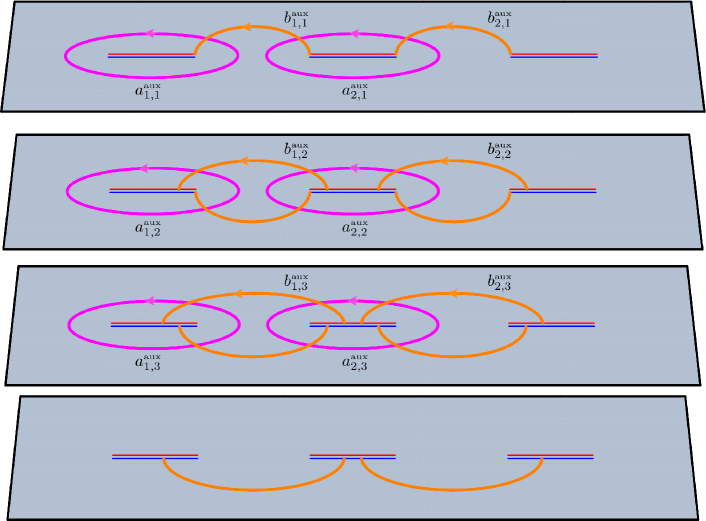
Figure 27: The auxiliary cycles $\{a^{\textrm{\tiny aux}}_{\alpha,j},b^{\textrm{\tiny aux}}_{\alpha,j}\}$ for $N=3$ and $n=4$.

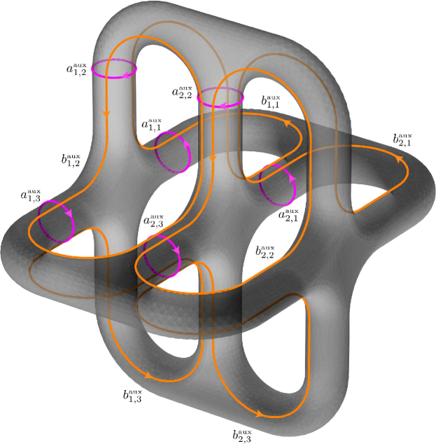
Figure 28: The Riemann surface $\mathscr{R}_{3,4}$ with the set of auxiliary cycles $\{a^{\textrm{\tiny aux}}_{\alpha,j},b^{\textrm{\tiny aux}}_{\alpha,j}\}$ depicted also in Fig. 27.

Appendix B Lauricella functions

In this appendix we show that the integrals (3.12) and (3.13), occurring in §3.1 and §4.2 for the computation of the period matrices, can be written in terms of the fourth Lauricella function $F_{D}^{(m)}$ [54], which is a generalization of the hypergeometric function ${}_{2}F_{1}$ involving several variables.

The integral representation of $F_{D}^{(m)}$ for $\textrm{Re}(c)>\textrm{Re}(a)>0$ reads

$$\int_{0}^{1}\frac{t^{a-1}(1-t)^{c-a-1}}{\prod_{j=1}^{m}(1-y_{j}t)^{b_{j}}}\,dt=\frac{\Gamma(a)\,\Gamma(c-a)}{\Gamma(c)}\,F_{D}^{(m)}(a,b_{1},\dots,b_{m};c\,;y_{1},\dots,y_{m})\,.$$ (B.1)

For $m=1$ the function $F_{D}^{(m)}$ reduces to the hypergeometric function ${}_{2}F_{1}(a,b_{1};c;y_{1})$ and for $m=2$ it becomes the Appell function $F_{1}(a;b_{1},b_{2};c;y_{1},y_{2})$. In our problem $m=2N-3$ and therefore $m\geqslant 3$ for $N>2$.

In terms of the Lauricella function, the integral in (3.12) for $\alpha=1$ reads

$$\mathscr{I}_{\beta,k}\big{|}_{0}^{x_{1}}=\,\frac{\Gamma(\beta-k/n)\,\Gamma(k/n)}{\Gamma(\beta)}\;x_{1}^{\beta-1}\prod_{\gamma=2}^{N-1}x_{2\gamma-2}^{-k/n}\,\prod_{\lambda=2}^{N-1}x_{2\lambda-1}^{k/n-1}$$ (B.2)

$$\hskip 51.21504pt\times F_{D}^{(2N-3)}\bigg{(}\beta-\frac{k}{n},\frac{k}{n},1-\frac{k}{n},\dots,\frac{k}{n};\beta\,;\frac{x_{1}}{x_{2}},\frac{x_{1}}{x_{3}},\dots,\frac{x_{1}}{x_{2N-2}}\bigg{)}\,,$$

where we recall that $x_{2N-2}=1$ and $1\leqslant\beta\leqslant N-1$. Also the remaining integrals in (3.12), which have $\alpha>1$, can be written through $F_{D}^{(m)}$

$$\mathscr{I}_{\beta,k}\big{|}_{x_{2\alpha-2}}^{x_{2\alpha-1}}=\,\frac{\pi}{\sin(\pi k/n)}\;x_{2\alpha-2}^{\beta-1-k/n}\prod_{\begin{subarray}{c}\gamma=2\\ \gamma\neq\alpha\end{subarray}}^{N}|x_{2\gamma-2}-x_{2\alpha-2}|^{-k/n}\prod_{\begin{subarray}{c}\lambda=1\\ \lambda\neq\alpha\end{subarray}}^{N-1}|x_{2\lambda-1}-x_{2\alpha-2}|^{k/n-1}$$

$$\hskip 51.21504pt\times F_{D}^{(2N-3)}\bigg{(}1-\frac{k}{n},\frac{k}{n}+1-\beta,1-\frac{k}{n},\dots,\frac{k}{n};1;\,\boldsymbol{y}^{(\alpha)}\bigg{)},$$ (B.3)

where $\Gamma(1-k/n)\,\Gamma(k/n)=\pi\csc(\pi k/n)$ has been used and we introduced the $2N-3$ dimensional vector $\boldsymbol{y}^{(\alpha)}$, whose elements read

$$y^{(\alpha)}_{\zeta}\equiv\frac{x_{2\alpha-1}-x_{2\alpha-2}}{x_{\zeta}-x_{2\alpha-2}}\,,\qquad\zeta\in\{0,1,\dots,2N-2\}\setminus\{2\alpha-2,2\alpha-1\}\,.$$ (B.4)

As for the integrals in (3.13) for $\alpha\geqslant 1$, in terms of Lauricella functions they become

$$\mathscr{I}_{\beta,k}\big{|}_{x_{2\alpha-1}}^{x_{2\alpha}}=\,\frac{\pi}{\sin(\pi k/n)}\;x_{2\alpha-1}^{\beta-1-k/n}\prod_{\begin{subarray}{c}\gamma=1\\ \gamma\neq\alpha\end{subarray}}^{N}|x_{2\gamma-2}-x_{2\alpha-2}|^{-k/n}\prod_{\begin{subarray}{c}\gamma=1\\ \gamma\neq\alpha\end{subarray}}^{N-1}|x_{2\gamma-1}-x_{2\alpha-2}|^{k/n-1}$$

$$\hskip 51.21504pt\times F_{D}^{(2N-3)}\bigg{(}\frac{k}{n},\frac{k}{n}+1-\beta,1-\frac{k}{n},\dots,\frac{k}{n};1;\,\boldsymbol{w}^{(\alpha)}\bigg{)},$$ (B.5)

where we defined the $2N-3$ dimensional vector $\boldsymbol{w}^{(\alpha)}$, whose elements are

$$w^{(\alpha)}_{\zeta}\equiv\frac{x_{2\alpha}-x_{2\alpha-1}}{x_{\zeta}-x_{2\alpha-1}}\,,\qquad\zeta\in\{0,1,\dots,2N-2\}\setminus\{2\alpha-1,2\alpha\}\,.$$ (B.6)

We remark that both in (B) and (B) the dots denote the alternating occurrence of $k/n$ and $1-k/n$, like in (B.2). For even $n$, the case $k/n=1/2$ occurs and these expressions slightly simplify. In order to realize that (B.2) is (B) with $\alpha=1$, it is more convenient to go back to the original integral representation and set $\alpha=1$ there.

For $N=2$ intervals we have only one harmonic ratio $x_{1}=x\in(0,1)$. Moreover, $\alpha=\beta=1$ and therefore we have to consider only (B.2) and (B), which reduce respectively to

$$\mathscr{I}_{1,k}\big{|}_{0}^{x} = \frac{\pi}{\sin(\pi k/n)}\,F_{k/n}(x)\,,$$ (B.7)

$$\mathscr{I}_{1,k}\big{|}_{x}^{1} = \frac{\pi}{\sin(\pi k/n)}\;x^{-k/n}\,_{2}F_{1}\bigg{(}\,\frac{k}{n},\frac{k}{n};1;\frac{x-1}{x}\bigg{)}=\;\frac{\pi}{\sin(\pi k/n)}\;F_{k/n}(1-x)\,,$$ (B.8)

being $F_{k/n}$ the hypergeometric function defined in (4.1). In the last step of (B.8) we have employed the Kummer’s relation $\,{}_{2}F_{1}(a,b;c;y)=(1-y)^{-a}\,_{2}F_{1}(a,c-b;c;y/(y-1))$.

Appendix C Symmetries of $\mathcal{F}_{N,n}$ as symplectic transformations

In this appendix we discuss some symmetries of $\mathcal{F}_{N,n}$ through the symplectic modular transformations. In Appendix C.1 we define the group $Sp(2g,\mathbb{Z})$ and its action on the Riemann theta functions, introducing the subset of transformations we are interested in. In Appendix C.2 we show that $\mathcal{F}_{N,n}$ is invariant under such class of modular transformations, for both the compactified boson and the Ising model, and in Appendix C.3 we construct the symplectic matrices implementing the cyclic transformation in the sequence of the sheets, the inversion of their order and the exchange $A\leftrightarrow B$.

C.1 The symplectic modular group

Let us consider the group $Sp(2g,\mathbb{Z})$ of the integer symplectic matrices, which is also known as symplectic modular group. The generic element $M\in Sp(2g,\mathbb{Z})$ is a $2g\times 2g$ matrix which satisfies

$$M=\begin{pmatrix}D&C\\ B&A\end{pmatrix},\qquad M^{\textrm{t}}\cdot J\cdot M=J\,,\qquad J=\begin{pmatrix}0_{g}&\mathbb{I}_{g}\\ -\mathbb{I}_{g}&0_{g}\end{pmatrix},$$ (C.1)

where the $g\times g$ matrices $A$, $B$, $C$ and $D$ are made of integers, $0_{g}$ is the $g\times g$ matrix whose elements are all equal to zero and $\mathbb{I}_{g}$ is the identity matrix. The condition in (C.1) on $M$ corresponds to require that $D^{\textrm{t}}\cdot B$ and $C^{\textrm{t}}\cdot A$ are symmetric matrices and also $D^{\textrm{t}}\cdot A-B^{\textrm{t}}\cdot C=\mathbb{I}_{g}$.

Under a symplectic transformation, the canonical basis of cycles and the normalized basis of the holomorphic one forms transform respectively as follows

$$\begin{pmatrix}\boldsymbol{a}^{\prime}\\ \boldsymbol{b}^{\prime}\end{pmatrix}=M\cdot\begin{pmatrix}\boldsymbol{a}\\ \boldsymbol{b}\end{pmatrix},\qquad\boldsymbol{\nu}^{\prime\,\textrm{t}}=\boldsymbol{\nu}^{\,\textrm{t}}\cdot(C\cdot\tau+D)^{-1}\,.$$ (C.2)

From the first transformation rule, it is straightforward to observe that a canonical homology basis is sent into another canonical homology basis. Moreover, combining the transformation rules in (C.2), one finds that the period matrix $\tau^{\prime}$ computed through $\boldsymbol{\nu}^{\prime}$ and the cycles $\boldsymbol{b}^{\prime}$ is related to $\tau$ in (3.6) as follows

$$\tau^{\prime}=(A\cdot\tau+B)\cdot(C\cdot\tau+D)^{-1}\,.$$ (C.3)

The transformation rule for the absolute value of the Riemann theta function with characteristic defined in (3.35) reads [9, 10, 11, 15, 16]

$$\big{|}\Theta[\boldsymbol{e}^{\prime}](\boldsymbol{0}|\tau^{\prime})\big{|}=\sqrt{|\textrm{det}(C\cdot\tau+D)|}\;\big{|}\Theta[\boldsymbol{e}](\boldsymbol{0}|\tau)\big{|}\,,$$ (C.4)

where the characteristic $\boldsymbol{e}^{\prime}$ is given by

$$\begin{pmatrix}\boldsymbol{\varepsilon}^{\prime}\\ \boldsymbol{\delta}^{\prime}\end{pmatrix}=\begin{pmatrix}D&-C\\ -B&A\end{pmatrix}\cdot\begin{pmatrix}\boldsymbol{\varepsilon}\\ \boldsymbol{\delta}\end{pmatrix}+\frac{1}{2}\,\begin{pmatrix}(C\cdot D^{\textrm{t}})_{\textrm{d}}\\ (A\cdot B^{\textrm{t}})_{\textrm{d}}\end{pmatrix},$$ (C.5)

where $(\dots)_{\textrm{d}}$ is the vector made by the diagonal of the matrix within the brackets.

Let us consider the subset of $Sp(2g,\mathbb{Z})$ given by the following matrices

$$\begin{pmatrix}D&0_{g}\\ 0_{g}&(D^{-1})^{\textrm{t}}\end{pmatrix},\qquad\begin{pmatrix}0_{g}&C\,\\ -(C^{-1})^{\textrm{t}}&0_{g}\end{pmatrix}.$$ (C.6)

Under the transformations of the first kind, the cycles $\boldsymbol{a}^{\prime}$ ($\boldsymbol{b}^{\prime}$) are obtained through $\boldsymbol{a}$ ($\boldsymbol{b}$) cycles only; while applying the transformations of the second kind, the cycles $\boldsymbol{a}^{\prime}$ ($\boldsymbol{b}^{\prime}$) are combinations of the cycles $\boldsymbol{b}$ ($\boldsymbol{a}$). Moreover, for the transformations (C.6) the relation (C.5) between the characteristics becomes homogenous. In particular, the zero characteristic is mapped into itself and therefore (C.4) becomes

$$\big{|}\Theta(\boldsymbol{0}|\tau^{\prime})\big{|}=\sqrt{|\textrm{det}(C\cdot\tau+D)|}\;\big{|}\Theta(\boldsymbol{0}|\tau)\big{|}\,.$$ (C.7)

In the remaining part of this appendix, we will restrict to the transformations (C.6).

C.2 Invariance of $\mathcal{F}_{N,n}$

Let us discuss the invariance of $\mathcal{F}_{N,n}(\boldsymbol{x})$ under (C.6) for the free compactified boson.
Considering the two expressions in (3.29) which are not explicitly invariant under $\eta\leftrightarrow 1/\eta$, one finds that $\sqrt{\textrm{det}(\mathcal{I})}\,|\Theta(\boldsymbol{0}|\tau)|^{2}$ and $\Theta(\boldsymbol{0}|\textrm{i}\eta G)$ (or $\Theta(\boldsymbol{0}|\textrm{i}G/\eta)$ equivalently) are separately invariant. The invariance of $\sqrt{\textrm{det}(\mathcal{I})}\,|\Theta(\boldsymbol{0}|\tau)|^{2}$ is easily obtained combining (C.7) and the following relation [11]

$$(\mathcal{I}^{\prime})^{-1}=(C\cdot\bar{\tau}+D)\cdot\mathcal{I}^{-1}\cdot(C\cdot\tau+D)^{\textrm{t}}\,,$$ (C.8)

which can be verified starting from (C.3). This allows us to claim that the expression $\mathcal{F}_{N,n}^{\eta\rightarrow\infty}(\boldsymbol{x})$ in (3.31), which characterizes the decompactification regime, is invariant under symplectic transformations.
As for the invariance $\Theta(\boldsymbol{0}|\textrm{i}\eta G)$, first we find it convenient to write $G$ in (3.28) as

$$G=\begin{pmatrix}\tau\cdot\mathcal{I}^{-1}\cdot\bar{\tau}&\;\tau\cdot\mathcal{I}^{-1}-\textrm{i}\,\mathbb{I}_{g}\,\\ \;\mathcal{I}^{-1}\cdot\bar{\tau}+\textrm{i}\,\mathbb{I}_{g}&\;\;\;\;\mathcal{I}^{-1}\end{pmatrix}.$$ (C.9)

The terms $\pm\textrm{i}\,\mathbb{I}_{g}$ in the off diagonal blocks can be dropped because they cancel each others in the exponent of the general term of the series defining $\Theta(\boldsymbol{0}|\textrm{i}\eta G)$. Then, we can employ the fact that $\Theta(\boldsymbol{0}|\textrm{i}\eta G)$ does not change under simultaneous inversion of the sign for both the off diagonal matrices in $G$. Considering the exponent of the general term of the series, after some algebra one finds that

$$\begin{pmatrix}\boldsymbol{m}^{\textrm{t}}&\boldsymbol{n}^{\textrm{t}}\end{pmatrix}\cdot\begin{pmatrix}\;\tau^{\prime}\cdot(\mathcal{I}^{\prime})^{-1}\cdot\bar{\tau}^{\prime}&\;-\,\tau^{\prime}\cdot(\mathcal{I}^{\prime})^{-1}\,\\ -(\mathcal{I}^{\prime})^{-1}\cdot\bar{\tau}^{\prime}&\;\;\;(\mathcal{I}^{\prime})^{-1}\end{pmatrix}\cdot\begin{pmatrix}\boldsymbol{m}\\ \boldsymbol{n}\end{pmatrix}$$ (C.10)

$$\;=\;\begin{pmatrix}\boldsymbol{m}^{\prime\,\textrm{t}}&\boldsymbol{n}^{\prime\,\textrm{t}}\end{pmatrix}\cdot\begin{pmatrix}\;\tau\cdot\mathcal{I}^{-1}\cdot\bar{\tau}&\;-\,\tau\cdot\mathcal{I}^{-1}\,\\ -\,\mathcal{I}^{-1}\cdot\bar{\tau}&\;\;\;\mathcal{I}^{-1}\end{pmatrix}\cdot\begin{pmatrix}\boldsymbol{m}^{\prime}\\ \boldsymbol{n}^{\prime}\end{pmatrix},$$

where $(\mathcal{I}^{\prime})^{-1}$ is defined in (C.8), $\tau^{\prime}$ in (C.3) and we also introduced

$$\begin{pmatrix}\boldsymbol{m}^{\prime}\\ \boldsymbol{n}^{\prime}\end{pmatrix}=M^{-1}\cdot\begin{pmatrix}\boldsymbol{m}\\ \boldsymbol{n}\end{pmatrix},\qquad M^{-1}=\begin{pmatrix}A^{\textrm{t}}&-\,C^{\textrm{t}}\\ -B^{\textrm{t}}&D^{\textrm{t}}\end{pmatrix}.$$ (C.11)

The vectors $\boldsymbol{m}^{\prime}$ and $\boldsymbol{n}^{\prime}$ are made of integers and they are related to $\boldsymbol{m}$ and $\boldsymbol{n}$ through the inverse $M^{-1}$ of symplectic transformation (C.1), which is also a symplectic matrix. Since also $(\boldsymbol{m}^{\prime\,\textrm{t}},\boldsymbol{n}^{\prime\,\textrm{t}})$ cover the whole $\mathbb{Z}^{2g}$, we have that $\Theta(\boldsymbol{0}|\textrm{i}\eta G)$ is invariant under $Sp(2g,\mathbb{Z})$ for any $\eta$.

For the Ising model, we have that $\mathcal{F}^{\textrm{\tiny Ising}}_{N,n}(\boldsymbol{x})$ in (6.2) is invariant under (C.6). Indeed, from (C.4) and (C.7) it is straightforward to conclude that

$$\bigg{|}\frac{\Theta[\boldsymbol{e}^{\prime}](\boldsymbol{0}|\tau^{\prime})}{\Theta(\boldsymbol{0}|\tau^{\prime})}\bigg{|}=\bigg{|}\frac{\Theta[\boldsymbol{e}](\boldsymbol{0}|\tau)}{\Theta(\boldsymbol{0}|\tau)}\bigg{|}\,.$$ (C.12)

Moreover, each term of the sum over the characteristics in (6.2) is sent into a different one (except for $\boldsymbol{e}^{\textrm{t}}=(\boldsymbol{0}^{\textrm{t}},\boldsymbol{0}^{\textrm{t}})$) so that the whole sum is invariant because the net effect of (C.6) is to reshuffle its terms.

C.3 Some explicit modular transformations

C.3.1 Cyclic transformation.

As a concrete example of a symmetry written in terms of a symplectic matrix, we consider first the cyclic change in the ordering of the sheets. Indeed, the choice of the first sheet is arbitrary and therefore the period matrix cannot depend on it. This symmetry has been already studied in [29].
It is useful to start from the effect of this transformation on the auxiliary cycles of Figs. 27 and 28: $a^{\textrm{\tiny aux}}_{\alpha,j}\rightarrow a^{\textrm{\tiny aux}}_{\alpha,j+1}$ and $b^{\textrm{\tiny aux}}_{\alpha,j}\rightarrow b^{\textrm{\tiny aux}}_{\alpha,j+1}$. Notice that we introduced the cycles $a^{\textrm{\tiny aux}}_{\alpha,n}\equiv a^{\textrm{\tiny aux}}_{\alpha,0}$ and $b^{\textrm{\tiny aux}}_{\alpha,n}\equiv b^{\textrm{\tiny aux}}_{\alpha,0}$, which are not shown in Figs. 27 and 28, but, given their indices, it is clear how to place them. In particular, considering this enlarged set of auxiliary cycles, we have that $\sum_{j=1}^{n}a^{\textrm{\tiny aux}}_{\alpha,j}=\sum_{j=1}^{n}b^{\textrm{\tiny aux}}_{\alpha,j}=0$, which allow to write $a^{\textrm{\tiny aux}}_{\alpha,n}$ and $b^{\textrm{\tiny aux}}_{\alpha,n}$ in terms of the other ones. From these relations and (3.8), we find that the canonical homology basis introduced in §3.1 changes as follows

$$a_{\alpha,j}\rightarrow a_{\alpha,j+1}\hskip 14.22636ptj\neq n-1\,,\qquad a_{\alpha,n-1}\rightarrow-\displaystyle\sum_{k=1}^{n-1}a_{\alpha,k}\,,\qquad b_{\alpha,j}\rightarrow b_{\alpha,j+1}-b_{\alpha,1}\,.$$ (C.13)

As for the canonical homology basis defined in §4.2, from (4.6) we have

$$\tilde{a}_{\alpha,j}\rightarrow\tilde{a}_{\alpha,j+1}-\tilde{a}_{\alpha,1}\,,\qquad\tilde{b}_{\alpha,j}\rightarrow\tilde{b}_{\alpha,j+1}\hskip 14.22636ptj\neq n-1\,,\qquad b_{\alpha,n-1}\rightarrow-\displaystyle\sum_{k=1}^{n-1}\tilde{b}_{\alpha,k}\,.$$ (C.14)

Since these transformations do not affect the greek index, their rewriting in a matrix form involves $\mathbb{I}_{N-1}$. In particular, (C.13) and (C.14) become respectively

$$M_{\text{cyc}}=\begin{pmatrix}D_{\text{cyc}}&0_{n-1}\\ 0_{n-1}&A_{\text{cyc}}\end{pmatrix}\otimes\mathbb{I}_{N-1}\,,\qquad\tilde{M}_{\text{cyc}}=\begin{pmatrix}\tilde{D}_{\text{cyc}}&0_{n-1}\\ 0_{n-1}&\tilde{A}_{\text{cyc}}\end{pmatrix}\otimes\mathbb{I}_{N-1}\,,$$ (C.15)

where

$$\bigg{\{}\begin{array}[]{l}(A_{\text{cyc}})_{jk}=\delta_{k-j,1}-\delta_{k,1}\\ (D_{\text{cyc}})_{jk}=\delta_{k-j,1}-\delta_{j,n-1}\end{array},\qquad\bigg{\{}\begin{array}[]{l}(\tilde{A}_{\text{cyc}})_{jk}=\delta_{k-j,1}-\delta_{j,n-1}=(D_{\text{cyc}})_{jk}\\ (\tilde{D}_{\text{cyc}})_{jk}=\delta_{k-j,1}-\delta_{k,1}=(A_{\text{cyc}})_{jk}\end{array}.$$ (C.16)

Since $A_{\text{cyc}}=(D_{\text{cyc}}^{-1})^{\textrm{t}}$, we have that $M_{\text{cyc}}$ and $\tilde{M}_{\text{cyc}}$ belong to subset of $Sp(2g,\mathbb{Z})$ defined by the first expression in (C.6). Notice that $(D_{\text{cyc}}^{-1})^{\textrm{t}}$ is the matrix given in Eq. (3.28) of [29]. Moreover, we checked that $M_{\text{cyc}}^{n}=\tilde{M}_{\text{cyc}}^{n}=\mathbb{I}_{2g}$ and also that $M_{\text{cyc}}=M^{-1}\cdot\tilde{M}_{\text{cyc}}\cdot M$, being $M$ the matrix defined in (4.13), which relates the two canonical homology bases. As for the period matrix, by applying (C.3) for the transformations (C.15), we numerically checked that $\tau^{\prime}_{\text{cyc}}(\boldsymbol{x})=\tau(\boldsymbol{x})$ and $\tilde{\tau}^{\prime}_{\text{cyc}}(\boldsymbol{x})=\tilde{\tau}(\boldsymbol{x})$, as expected.

C.3.2 Inversion.

Another symmetry that we can consider is obtained by taking the sheets in the inverse order. As above, we start from the action of this transformation on the auxiliary cycles, which is $a^{\textrm{\tiny aux}}_{\alpha,j}\rightarrow-a^{\textrm{\tiny aux}}_{\alpha,n-j+1}$ and $b^{\textrm{\tiny aux}}_{\alpha,j}\rightarrow b^{\textrm{\tiny aux}}_{\alpha,n-j}$ (we assume the enlarged set of auxiliary cycles introduced in Appendix C.3.1), where the opposite sign has been introduced to preserve the correct intersection number. Then, plugging it into (3.8), one finds that it acts on the canonical homology basis as follows

$$a_{\alpha,1}\rightarrow\sum_{k=1}^{n-1}a_{\alpha,k}\,,\qquad a_{\alpha,j}\rightarrow-a_{\alpha,n-j+1}\hskip 14.22636ptj\neq 1\,,\qquad b_{\alpha,j}\rightarrow b_{\alpha,1}-b_{\alpha,n-j+1}\,,$$ (C.17)

while, from (4.6), we get that the action on the canonical homology basis introduced in §4.2 is simply $\tilde{a}_{\alpha,j}\rightarrow\tilde{a}_{\alpha,n-j}$ and $\tilde{b}_{\alpha,j}\rightarrow\tilde{b}_{\alpha,n-j}$. The corresponding symplectic matrices $M_{\text{inv}}$ and $\tilde{M}_{\text{inv}}$ have the structure of (C.15) with

$$(A_{\text{inv}})_{jk}=(D^{\textrm{t}}_{\text{inv}})_{jk}=\delta_{k,1}-\delta_{j+k-1,n}\,,\qquad(\tilde{A}_{\text{inv}})_{jk}=(\tilde{D}_{\text{inv}})_{jk}=\delta_{j,n-k}\,.$$ (C.18)

They are related as $M_{\text{inv}}=M^{-1}\cdot\tilde{M}_{\text{inv}}\cdot M$, with $M$ is given by (4.13), as expected. A transformation very close to the one we are considering has been already studied in [29]. In particular, their Eq. (3.29) is given $A^{\textrm{t}}_{\text{inv}}$ up to a global minus sign and a cyclic transformation. Since the inversion is involutive, we have $M_{\text{inv}}^{2}=\tilde{M}_{\text{inv}}^{2}=\mathbb{I}_{2g}$.
As for the period matrix, from (C.3) we numerically find $\tau^{\prime}_{\text{inv}}(\boldsymbol{x})=-\,\bar{\tau}(\boldsymbol{x})$ and similarly, for the canonical basis of §4.2, we have $\tilde{\tau}^{\prime}_{\text{inv}}(\boldsymbol{x})=-\,\bar{\tilde{\tau}}(\boldsymbol{x})$. Since the imaginary part of the period matrix is left invariant, the inversion leaves the period matrix invariant only for $N=2$ or $n=2$ [29].

C.3.3 Exchange $A\leftrightarrow B$.

The transformations considered in Appendices C.3.1 and C.3.2 do not change the positions of the branch points. This means that $\boldsymbol{x}_{\text{cyc}}=\boldsymbol{x}_{\text{inv}}=\boldsymbol{x}$. Instead, exchanging $A=\cup_{i=1}^{N}A_{1}$ with its complement $B$, we move the intervals and this leads to a change of the harmonic ratios $\boldsymbol{x}$.

A way to implement the transformation $A\leftrightarrow B$ is given by

$$\left\{\begin{array}[]{l}A_{i}\,\rightarrow\,B_{i}\\ B_{i}\,\rightarrow\,A_{i+1\;\textrm{mod}\;N}\end{array}\right.,\qquad\left\{\begin{array}[]{l}u_{i}\,\rightarrow\,v_{i}\\ v_{i}\,\rightarrow\,u_{i+1\;\textrm{mod}\;N}\end{array}\right.,$$ (C.19)

where $i=1,\dots,N$. Applying this transformation twice, $A\rightarrow A$ and $B\rightarrow B$, but their components do not go back to themselves when $N>2$. Indeed, we have $A_{i}\rightarrow A_{i+2\,\textrm{mod}\,N}$ and $B_{i}\rightarrow B_{i+2\,\textrm{mod}\,N}$. Moreover, if we give to the intervals $A_{i}$ and $B_{i}$ an orientation, the transformation (C.19) does not change it. Indeed, twist fields $\mathcal{T}_{n}$ are sent into $\bar{\mathcal{T}}_{n}$ and viceversa. Under (C.19), the components of the vector $\boldsymbol{x}$ change as follows

$$x_{\zeta}\;\rightarrow\;1-\frac{x_{1}}{x_{\zeta+1}}\,,\qquad\zeta=1,\dots,2N-3\,,$$ (C.20)

i.e. $\boldsymbol{x}\rightarrow\boldsymbol{x}_{\text{ex,1}}$, where $(\boldsymbol{x}_{\text{ex,1}})_{\zeta}\equiv 1-x_{1}/x_{\zeta+1}$ (we recall that $x_{2N-2}\equiv 1$).
In order to describe the effect of (C.19) on the auxiliary cycles of Figs. 27 and 28, we find it useful to introduce, besides the $a^{\textrm{\tiny aux}}_{\alpha,n}$ and $b^{\textrm{\tiny aux}}_{\alpha,n}$ already defined in Appendix C.3.1, also the auxiliary cycles $a^{\textrm{\tiny aux}}_{N,j}$ and $b^{\textrm{\tiny aux}}_{N,j}$, so that $\sum_{\alpha=1}^{N}a^{\textrm{\tiny aux}}_{N,j}=\sum_{\alpha=1}^{N}b^{\textrm{\tiny aux}}_{N,j}=0$, where $j=1,\dots,n$. Considering this enlarged set of auxiliary cycles $\{a^{\textrm{\tiny aux}}_{\alpha,j},b^{\textrm{\tiny aux}}_{\alpha,j}\}$ where $\alpha=1,\dots,N$ and $j=1,\dots,n$, we find that (C.19) leads to $a^{\textrm{\tiny aux}}_{\alpha,j}\rightarrow b^{\textrm{\tiny aux}}_{\alpha,j}$ and $b^{\textrm{\tiny aux}}_{\alpha,j}\rightarrow-a^{\textrm{\tiny aux}}_{\alpha+1,j+1}$. By employing these relations in (3.8) and (4.6), we find respectively

$$\Bigg{\{}\begin{array}[]{l}a_{\alpha,j}\rightarrow\sum_{\gamma=1}^{\alpha}(b_{\gamma,j}-b_{\gamma,j+1})\\ \rule{0.0pt}{14.22636pt}b_{\alpha,j}\rightarrow\sum_{k=1}^{j}(a_{\alpha+1,k}-a_{\alpha,k})\end{array},\qquad\Bigg{\{}\begin{array}[]{l}\tilde{a}_{\alpha,j}\rightarrow\sum_{\gamma=1}^{\alpha}\sum_{k=1}^{j}\tilde{b}_{\gamma,k}\\ \rule{0.0pt}{14.22636pt}\tilde{b}_{\alpha,j}\rightarrow-\,\tilde{a}_{\alpha+1,j+1}+\tilde{a}_{\alpha+1,j}+\tilde{a}_{\alpha,j+1}-\tilde{a}_{\alpha,j}\end{array},$$ (C.21)

which can be written in matrix form respectively as

$$M_{\text{ex,1}}=\begin{pmatrix}0_{g}&-(I_{n-1}^{\textrm{\tiny up}})^{-1}\otimes I_{N-1}^{\textrm{\tiny low}}\\ \,I_{n-1}^{\textrm{\tiny low}}\otimes(I_{N-1}^{\textrm{\tiny up}})^{-1}&0_{g}\end{pmatrix},$$ (C.22)

and

$$\tilde{M}_{\text{ex,1}}=\begin{pmatrix}0_{g}&I_{n-1}^{\textrm{\tiny low}}\otimes I_{N-1}^{\textrm{\tiny low}}\\ \,-(I_{n-1}^{\textrm{\tiny up}})^{-1}\otimes(I_{N-1}^{\textrm{\tiny up}})^{-1}&0_{g}\end{pmatrix}.$$ (C.23)

Applying (C.3) for this transformation, we find $\tau^{\prime}_{\text{ex,1}}(\boldsymbol{x})=-\,\bar{\tau}(\boldsymbol{x}_{\text{ex,1}})$ and, for the canonical basis discussed in §4.2, $\tilde{\tau}^{\prime}_{\text{ex,1}}(\boldsymbol{x})=-\,\bar{\tilde{\tau}}(\boldsymbol{x}_{\text{ex,1}})$. Given the transformation of the period matrix under the inversion discussed in Appendix C.3.2, applying first (C.19) and then the inversion, we get $\tau^{\prime}_{\text{ex,1}}(\boldsymbol{x})=\tau(\boldsymbol{x}_{\text{ex,1}})$ and similarly for the tilded basis.

Another way to implement $A\leftrightarrow B$ is the following

$$\left\{\begin{array}[]{l}A_{i}\,\rightarrow\,B_{N-i\;\textrm{mod}\;N}\\ B_{i}\,\rightarrow\,A_{N-i\;\textrm{mod}\;N}\end{array},\right.\qquad\left\{\begin{array}[]{l}u_{i}\,\rightarrow\,u_{N-i+1}\\ v_{i}\,\rightarrow\,v_{N-i\;\textrm{mod}\;N}\end{array},\right.$$ (C.24)

which is an involution for each component $A_{i}$ and $B_{i}$. This map inverts the orientation of all the intervals and it sends a twist field $\mathcal{T}_{n}$ into another field of the same kind, and similarly for $\bar{\mathcal{T}}_{n}$. The change induced on $\boldsymbol{x}$ reads

$$x_{\zeta}\;\rightarrow\;1-x_{2N-2-\zeta}\equiv(\boldsymbol{x}_{\text{ex,2}})_{\zeta}\,,\qquad\zeta=1,\dots,2N-3\,.$$ (C.25)

When $N=2$, both (C.20) and (C.25) give $x\rightarrow 1-x$. The transformation (C.24) acts on the enlarged set of auxiliary cycles described above as $a^{\textrm{\tiny aux}}_{\alpha,j}\rightarrow b^{\textrm{\tiny aux}}_{N-\alpha,j}$ and $b^{\textrm{\tiny aux}}_{\alpha,j}\rightarrow a^{\textrm{\tiny aux}}_{N-\alpha,j+1}$. Through (3.8) and (4.6), this allows us to find respectively

$$\Bigg{\{}\begin{array}[]{l}a_{\alpha,j}\rightarrow\sum_{\gamma=N-\alpha}^{N-1}(b_{\gamma,j-1}-b_{\gamma,j})\\ \rule{0.0pt}{14.22636pt}b_{\alpha,j}\rightarrow\sum_{k=j}^{n-1}(a_{N-\alpha,k}-a_{N-\alpha-1,k})\end{array},$$ (C.26)

and

$$\Bigg{\{}\begin{array}[]{l}\tilde{a}_{\alpha,j}\rightarrow\sum_{\gamma=N-\alpha}^{N-1}\sum_{k=1}^{j}\tilde{b}_{\gamma,k}\\ \rule{0.0pt}{14.22636pt}\tilde{b}_{\alpha,j}\rightarrow\tilde{a}_{N-\alpha,j+1}-\tilde{a}_{N-\alpha,j}-\tilde{a}_{N-\alpha-1,j+1}+\tilde{a}_{N-\alpha-1,j}\end{array},$$ (C.27)

whose expressions in matrix form read

$$M_{\text{ex,2}}=\begin{pmatrix}0_{g}&-(I_{n-1}^{\textrm{\tiny low}})^{-1}\otimes\check{I}_{N-1}^{\textrm{\tiny low}}\\ \,I_{n-1}^{\textrm{\tiny up}}\otimes(\check{I}_{N-1}^{\textrm{\tiny up}})^{-1}&0_{g}\end{pmatrix},$$ (C.28)

and

$$\tilde{M}_{\text{ex,2}}=\begin{pmatrix}0_{g}&I_{n-1}^{\textrm{\tiny low}}\otimes\check{I}_{N-1}^{\textrm{\tiny low}}\\ \,-(I_{n-1}^{\textrm{\tiny up}})^{-1}\otimes(\check{I}_{N-1}^{\textrm{\tiny low}})^{-1}&0_{g}\end{pmatrix},$$ (C.29)

where $(\check{I}_{N-1})_{\alpha\beta}\equiv 1$ if $\alpha\geqslant N-\beta$ and $(\check{I}_{N-1})_{\alpha\beta}\equiv 0$ otherwise. As for the change of the period matrix under (C.25), applying the transformation rule (C.3) for (C.28) and (C.29), we find $\tau^{\prime}_{\text{ex,2}}(\boldsymbol{x})=\tau(\boldsymbol{x}_{\text{ex,2}})$ and $\tilde{\tau}^{\prime}_{\text{ex,2}}(\boldsymbol{x})=\tilde{\tau}(\boldsymbol{x}_{\text{ex,2}})$ respectively.

We remark that, under the transformations considered in this subsection, the ratio within the absolute value in (2.7) is left invariant. Indeed, the cyclic transformation and the inversion do not involve the endpoints of the intervals at all. As for $A\leftrightarrow B$, in the two cases shown above, either the sets $\{u_{i},i=1,\dots,N\}$ and $\{v_{i},i=1,\dots,N\}$ are exchanged or they are mapped into themselves.

Appendix D Some technical issues on the numerical analysis

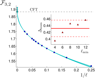
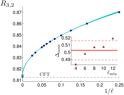
Figure 29: Leading corrections to the scaling of $\mathcal{F}_{3,2}$ (left) and $R_{3,2}$ (right) for the special case of $\alpha=0.5$ and $x_{1}=0.146$ (see top right of Figs. 24 and 25), computed as explained in Appendix D.1. In the inset we show the mean value of $\Delta_{\textrm{num}}$ and the error bars, obtained by fitting the data with the highest values of $\ell$, starting from $\ell_{\textrm{min}}$. Each fit provides a curve in the plot. The extrapolated values are show as cyan diamonds.

In this appendix we discuss some technical issues employed to extract the results of §6.4, performing also some additional analysis. In Appendices D.1 and D.2 we explain how the finite size scaling analysis has been performed by using either one correction or higher order ones, respectively. In Appendix D.3 we briefly discuss some effects due to the finiteness of the bond dimension.

D.1 The exponent in the first correction

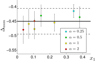
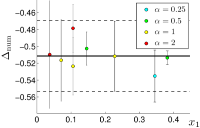
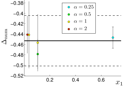
Figure 30: The value of the exponent $\Delta_{\textrm{num}}$ obtained from the numerical values of $\mathcal{F}_{3,2}$, $R_{3,2}$ and $\mathcal{F}_{4,2}$ (clockwise direction, starting from the top left). The values of $x_{1}$ correspond to the ones where several numerical points are available (see Figs. 24, 25 and 26 respectively). The error bars are obtained by changing the number of numerical points in the fit (see Fig. 29).

Given the large discrepancy between our numerical data for the Ising model and the corresponding CFT predictions, the finite size scaling analysis becomes crucial either to confirm or to discard them. As discussed in §6.4, we numerically study ${\rm Tr}\rho_{A}^{2}$ when $A$ is made by three or four disjoint intervals by considering ${\cal F}_{3,2}$, $R_{3,2}$ and ${\cal F}_{4,2}$.

The first step in the finite size scaling analysis is the determination of the exponents of the corrections. To this aim, we start by taking only one correction into account. Since we usually have only few numerical points for a fixed value of $\boldsymbol{x}$, let us focus on those $\boldsymbol{x}$’s with several of them coming from different values of $\chi$. For these $\boldsymbol{x}$’s, which correspond to different $\alpha$’s, we fit the numerical data for ${\cal F}_{3,2}$, $R_{3,2}$ and ${\cal F}_{4,2}$ by using the function $a_{0}+b_{0}/\ell^{\Delta_{\textrm{num}}}$, which has three parameters to determine. Changing the ranges of variation for $\ell$, we can check the stability of the results and also find an estimate of the error for the fitting process (see Fig. 29 for a typical example). The results for $\Delta_{\textrm{num}}$ are shown in Fig. 30: starting from the top left in clockwise direction, we find $\Delta_{\textrm{num}}=0.45(5)$, $\Delta_{\textrm{num}}=0.51(4)$ and $\Delta_{\textrm{num}}=0.45(5)$ for ${\cal F}_{3,2}$, $R_{3,2}$ and ${\cal F}_{4,2}$ respectively. In this analysis the CFT formulas have not been used. Notice that it is non trivial that $\Delta_{\textrm{num}}$ does not depend on $\boldsymbol{x}$. Our results are consistent with $\Delta_{\textrm{num}}=1/2$ found for $N=2$ [20, 22] and they show that it holds also for $N>2$.

The values of $\Delta_{\textrm{num}}$ just given have been used in (6.10) to find the extrapolated points in Figs. 24, 25 and 26. Thus, for each $\boldsymbol{x}$, now there are two parameters to fit. Notice that we have not employed the CFT formula yet.

In Fig. 31 we plot the difference between the numerical data and the CFT prediction in log-log scale, in order to visualize the leading correction. All the data lie on parallel lines whose slope is close to the one expected from the two intervals case.

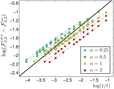
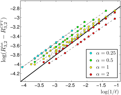
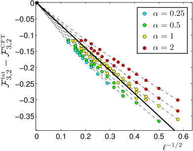
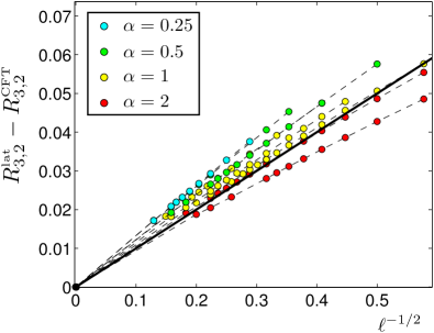
Figure 31: Difference between the numerical data and the CFT prediction for $\mathcal{F}_{3,2}$ (left) and $R_{3,2}$ (right). The black solid line corresponds to $\Delta=1/2$ for the exponent of the leading correction, which is the value expected from CFT arguments. In the upper panels the results are shown in logarithmic scales in order to appreciate the fact that, joining the data having the same $\boldsymbol{x}$, we find almost straight lines having nearly the same slope.

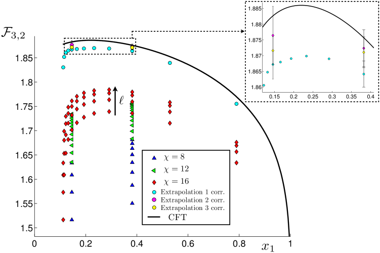
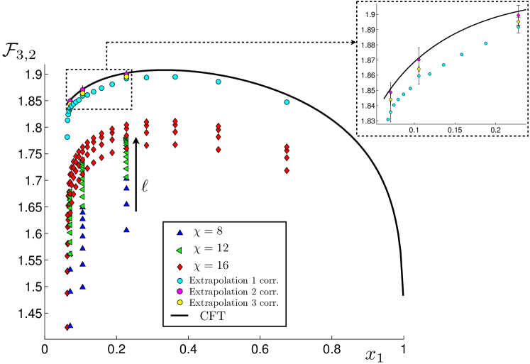
Figure 32: Finite size scaling analysis with higher order corrections for $\mathcal{F}_{3,2}$ for the configurations characterized by $\alpha=0.5$ (top) and $\alpha=1$ (bottom). The method is explained in Appendix D.2. Three corrections can be taken into account only for those $\boldsymbol{x}$’s having several numerical points, as shown in the zoom. The third correction never improves the agreement with the CFT prediction.

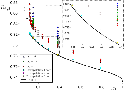
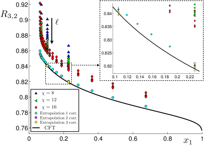
Figure 33: Finite size scaling analysis with higher order corrections for $R_{3,2}$ for the configurations characterized by $\alpha=0.5$ (left) and $\alpha=1$ (right). The method is explained in Appendix D.2. Three corrections can be taken into account only for those $\boldsymbol{x}$’s having several numerical points, as shown in the zoom. The third correction never improves the agreement with the CFT prediction.

D.2 A finite size scaling analysis with higher order corrections

Instead of considering only one correction as discussed in §6.4 and Appendix D.1, one can try to perform a finite size scaling analysis which includes more corrections [84, 85, 20, 22, 23, 39]. In particular, we choose the following function

$$a_{0}+\frac{b_{1}}{\ell^{1/2}}+\frac{b_{2}}{\ell}+\frac{b_{3}}{\ell^{3/2}}\,.$$ (D.1)

The exponents are the ones giving agreement with the CFT predictions for $N=2$ [39]. Since in this case we have four parameters to fit, we can carry out this analysis only for few $\boldsymbol{x}$’s at fixed $\alpha$. We have considered the same configurations of §6.4, namely $\alpha=p$ and $\alpha=1/p$ with $1\leqslant p\leqslant 8$ finding the same qualitative behavior. Here we give only one representative example in Fig 32 for $\mathcal{F}_{3,2}$ and in Fig 33 for $R_{3,2}$. The error bars have been determined by choosing different minimum values for $\ell$ in the fitting procedure, as done for $\Delta_{\textrm{num}}$ in Appendix D.1.

It is instructive to analyze the contribution of the various corrections. Taking only the first correction into account (cyan circles in Figs. 32 and 33), the extrapolated points are very close to the curves predicted by the CFT. Nevertheless, they do not coincide with it, staying systematically below for $\mathcal{F}_{N,2}$ or above for $R_{N,2}$. Adding the second correction, i.e. $b_{1}\neq 0$ and $b_{2}\neq 0$ in (D.1), the extrapolations (green circles in Figs. 32 and 33) usually improve, as expected, getting closer to the CFT prediction and, in some case, coinciding with it. As for the third correction, we notice that it does not improve the extrapolation in almost all the cases that we studied. This probably tells us that the range of $\ell$ available allows us to see at most two corrections to the scaling. As for the sign of the coefficients $b_{1}$, $b_{2}$ and $b_{3}$ in (D.1), we find $(-,+,+)$ for $\mathcal{F}_{3,2}$ and $(+,-,+)$ for $R_{3,2}$. Notice that the sign of $b_{1}$ can be easily inferred from the position of the numerical points with respect to the CFT curve. For instance, since for $R_{3,2}$ they are all above the theoretical curve, we have that $b_{1}>0$ in this case.

D.3 On the finiteness of the bond dimension

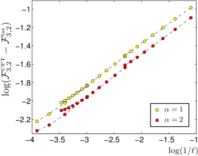
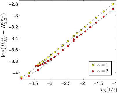
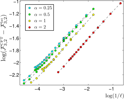
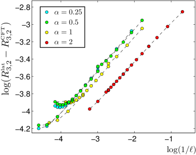
Figure 34: Effects of the finite bond dimension leading to deviations from the power law decays are shown for $\mathcal{F}_{3,2}$ (left) and $R_{3,2}$ (right). In the top panels $x_{1}=0.106$. For fixed $\ell$, the deviation from the straight line is more evident for points with larger $d$ ($\alpha=2$). In the bottom panels we have: $x_{1}=0.345$ ($\alpha=0.25$), $x_{1}=0.382$ ($\alpha=0.5$), $x_{1}=0.228$ ($\alpha=1$) and $x_{1}=0.037$ ($\alpha=2$). For small values of $\alpha$, regimes of large $\ell$ can be considered, where deviations may also occur. The points deviating from the straight line have been discarded from the numerical analysis.

Tensor networks, which include the MPS as a subclass, are variational approximations whose accuracy strongly depends on the bond dimension $\chi$. In principle, one would like to have access to the regime of $\chi\to\infty$ but, being the computational cost an increasing function of $\chi$, the results are always obtained for finite $\chi$.

The MPS are finitely correlated state, which means that they naturally describe systems where either the correlations do not decay or they decay exponentially at large distance [88]. The two cases are distinguished by the ratio $e_{2}/e_{1}\leqslant 1$ between the two largest eigenvalues $e_{1}$ and $e_{2}$ of the MPS transfer matrix $E$. In particular, if $e_{2}<e_{1}$, the finite correlation length of the MPS is $\xi_{\textrm{\tiny MPS}}\equiv 1/\log(e_{1}/e_{2})$, while, when $e_{2}=e_{1}$, the correlation function (6.6) is constant as a function of $r$ (long range order).

The finite size of a critical system naturally induces a finite correlation length $\xi_{L}\propto L$. Thus, the MPS representation can still be used to perform accurate finite size scaling analysis [71] and one would expect that a good MPS approximation has $\xi_{\textrm{\tiny MPS}}=\xi_{L}$. However, it has been found that, when $\chi$ is too small, the best approximation of a critical system through a MPS with finite $\chi$ has a finite correlation length $\xi_{\textrm{\tiny MPS}}=\xi_{\chi}\propto\chi^{\kappa}$ [72]. In order to get $\xi_{\textrm{\tiny MPS}}=\xi_{L}$, one needs to increase $\chi$. Since $\xi_{L}$ enters in the scaling of the two point correlation functions for critical systems, a useful criterion is obtained by considering [79, 74]

$$\chi^{\ast}=\min\big{\{}\chi\,\big{|}\,\xi_{\chi}>L/2\big{\}}\,.$$ (D.2)

However, notice that this result has been found by considering the two point functions of local operators, while in our problem both non local operators (whose support is of order $\xi_{\chi}$) and $2N\geqslant 4$ point functions are involved. In our numerical analysis we have adopted the criterion (D.2) and, indeed, we find that sometimes it fails. For instance, this happens in Fig. 34 whenever a deviation from the straight lines occurs. We have taken this failure into account by discarding from the numerical analysis the points deviating from the straight lines. Being (D.2) too optimistic for our computations, the criterion

$$\chi^{\ast}=\min\big{\{}\chi\,\big{|}\,\xi_{\chi}>L\big{\}}$$ (D.3)

should be enough to avoid deviations from the expected power law decay and should be implemented in future studies.

References

References

- [1] L. Amico, R. Fazio, A. Osterloh and V. Vedral, Entanglement in many-body systems, Rev. Mod. Phys. 80, 517 (2008); J. Eisert, M. Cramer and M. B. Plenio, Area laws for the entanglement entropy - a review, Rev. Mod. Phys. 82, 277 (2010); Entanglement entropy in extended quantum systems, P. Calabrese, J. Cardy and B. Doyon Eds, J. Phys. A 42, 500301 (2009).
- [2] C. Holzhey, F. Larsen and F. Wilczek, Geometric and renormalized entropy in conformal field theory, Nucl. Phys. B 424, (1994) 443.
- [3] P. Calabrese and J. Cardy, Entanglement entropy and quantum field theory, J. Stat. Mech. (2004) P06002.
- [4] P. Calabrese and J. Cardy, Entanglement entropy and conformal field theory, J. Phys. A 42, (2009) 504005.
- [5] P. Calabrese, J. Cardy and E. Tonni, Entanglement entropy of two disjoint intervals in conformal field theory, J. Stat. Mech. (2009) P11001.
- [6] P. Calabrese, J. Cardy and E. Tonni, Entanglement entropy of two disjoint intervals in conformal field theory II, J. Stat. Mech. (2011) P01021.
- [7] Al. B. Zamolodchikov, Conformal scalar field on the hyperelliptic curve and critical Ashkin-Teller multipoint correlation functions, Nucl. Phys. B 285 (1987) 481.
- [8] L. J. Dixon, D. Friedan, E. J. Martinec and S. H. Shenker, The Conformal Field Theory of Orbifolds, Nucl. Phys. B 282 (1987) 13.
- [9] L. Alvarez-Gaumé, G. W. Moore and C. Vafa, Theta Functions, Modular Invariance and Strings, Commun. Math. Phys. 106 1 (1986).
- [10] E. Verlinde and H. Verlinde, Chiral bosonization, determinants and the string partition function, Nucl. Phys. B 288 (1987) 357.
- [11] L. Alvarez-Gaumé, J.-B. Bost, G. W. Moore, P. Nelson and C. Vafa, Bosonization on Higher Genus Riemann Surfaces, Commun. Math. Phys. 112, 503 (1987).
- [12] V. Knizhnik, Analytic Fields on Riemann Surfaces II, Commun. Math. Phys. 112, 567 (1987).
- [13] M. Bershadsky and A. Radul, Conformal Field Theories with Additional Symmetry, Int. J. Mod. Phys. A02, 165 (1987).
- [14] R. Dijkgraaf, E. Verlinde and H. Verlinde, Conformal Field Theories on Riemann Surfaces, Commun. Math. Phys. 115 649 (1988).
- [15] J. Fay, Theta functions on Riemann surfaces, Lecture Notes in Mathematics 352, Springer-Verlag, 1973.
- [16] D. Mumford, Tata lectures on Theta III, Progress in Mathematics 97, Birkhäuser, Boston (1991).
- [17] J. Igusa, Theta Functions, Springer-Verlag, 1972.
- [18] M. Caraglio and F. Gliozzi, Entanglement entropy and twist fields, JHEP 0811: 076 (2008).
- [19] S. Furukawa, V. Pasquier, and J. Shiraishi, Mutual Information and Boson Radius in a Critical Systems in One Dimension, Phys. Rev. Lett. 102, 170602 (2009).
- [20] V. Alba, L. Tagliacozzo and P. Calabrese, Entanglement entropy of two disjoint blocks in critical Ising models, Phys. Rev. B 81, 060411 (2010).
- [21] F. Gliozzi and L. Tagliacozzo, Entanglement entropy and the complex plane of replicas, J. Stat. Mech. P01002 (2010).
- [22] M. Fagotti and P. Calabrese, Entanglement entropy of two disjoint blocks in XY chains, J. Stat. Mech. (2010) P04016.
- [23] V. Alba, L. Tagliacozzo, and P. Calabrese, Entanglement entropy of two disjoint intervals in theories, J. Stat. Mech. (2011) P06012.
- [24] M. Fagotti, New insights into the entanglement of disjoint blocks, EPL 97, 17007 (2012).
- [25] M. Rajabpour and F. Gliozzi, Entanglement entropy of two disjoint intervals from fusion algebra of twist fields, J. Stat. Mech. (2012) P02016.
- [26] H. Casini, C. Fosco and M. Huerta, Entanglement and alpha entropies for a massive Dirac field in two dimensions, J. Stat. Mech. (2010) P07007.
- [27] H. Casini and M. Huerta, Remarks on the entanglement entropy for disconnected regions, JHEP 0903:048 (2009).
- [28] H. Casini and M. Huerta, Reduced density matrix and internal dynamics for multicomponent regions, Class. Quant. Grav. 26, 185005 (2009).
- [29] M. Headrick, A. Lawrence and M. Roberts, Bose-Fermi dualities and entanglement entropies, J. Stat. Mech. (2012) P02022.
- [30] V. Enolski and T. Grava, Singular curves and Riemann-Hilbert problem, Int. Math. Res. Not. 32, (2004) 1619.
- [31] D. Perez-Garcia, F. Verstraete, M. M. Wolf and J. I. Cirac Matrix Product State Representations, Quantum Inf. Comput. 7, 401 (2007).
- [32] G. Evenbly and G. Vidal, Tensor network states and geometry, J. Stat. Phys. (2011) 145:891.
- [33] G. Vidal and R. F. Werner, A computable measure of entanglement, Phys. Rev. A 65, 032314 (2002).
- [34] K. Audenaert, J. Eisert, M. B. Plenio and R. F. Werner, Entanglement Properties of the Harmonic Chain, Phys. Rev. A 66, 042327 (2002).
- [35] P. Calabrese, J. Cardy and E. Tonni, Entanglement negativity and quantum field theory, Phys. Rev. Lett. 109, 130502 (2012).
- [36] P. Calabrese, J. Cardy and E. Tonni, Entanglement negativity in extended systems: a quantum field theory approach, J. Stat. Mech. (2013) P02008.
- [37] H. Wichterich, J. Molina-Vilaplana and S. Bose, Scaling of entanglement between separated blocks in spin chain at criticality, Phys. Rev. A 80, 010304(R) (2009).
- [38] V. Alba, Entanglement negativity and conformal field theory: a Monte Carlo study, J. Stat. Mech. (2013) P05013.
- [39] P. Calabrese, L. Tagliacozzo and E. Tonni, Entanglement negativity in the critical Ising chain, J. Stat. Mech. (2013) P05002.
- [40] S. Ryu and T. Takayanagi, Holographic derivation of entanglement entropy from AdS/CFT, Phys. Rev. Lett. 96, 181602 (2006).
- [41] S. Ryu and T. Takayanagi, Aspects of holographic entanglement entropy, JHEP 0608:045 (2006).
- [42] T. Takayanagi, Entanglement Entropy from a Holographic Viewpoint, Class. Quant. Grav. 29, (2012) 153001.
- [43] M. Headrick and T. Takayanagi, A holographic proof of the strong subadditivity of entanglement entropy, Phys. Rev. D 76, 106013 (2007).
- [44] V. E. Hubeny and M. Rangamani, Holographic entanglement entropy for disconnected regions, JHEP 0803:006 (2008).
- [45] M. Headrick, Entanglement Renyi entropies in holographic theories, Phys. Rev. D 82, 126010 (2010).
- [46] E. Tonni, Holographic entanglement entropy: near horizon geometry and disconnected regions, JHEP 1105:004 (2011).
- [47] P. Hayden, M. Headrick and A. Maloney, Holographic mutual information is monogamous, Phys. Rev. D 87, 046003 (2013).
- [48] H. Casini, M. Huerta and R. Myers, Towards a derivation of holographic entanglement entropy, JHEP 1105:036 (2011).
- [49] L. Hung, R. Myers, M. Smolkin and A. Yale, Holographic calculations of Rényi entropy, JHEP 1112:047 (2011).
- [50] T. Hartman, Entanglement Entropy at Large Central Charge, [1303.6955].
- [51] T. Faulkner, The Entanglement Renyi Entropies of Disjoint Intervals in AdS/CFT, [1303.7221].
- [52] A. Lewkowycz and J. Maldacena, Generalized gravitational entropy, [1304.4926].
- [53] J. L. Cardy, O. A. Castro-Alvaredo, and B. Doyon, Form factors of branch-point twist fields in quantum integrable models and entanglement entropy, J. Stat. Phys. 130 129 (2008).
- [54] H. Exton, Multiple hypergeometric functions and applications, Ellis Horwood, Chichester, 1976.
- [55] V. Enolski and T. Grava, Thomae type formulae for singular curves, Lett. Math. Phys. 76, (2006) 187.
- [56] I. Peschel and M. C. Chung, Density Matrices for a Chain of Oscillators, J. Phys. A 32, (1999) 8419.
- [57] I. Peschel, Calculation of reduced density matrices from correlation functions, J. Phys. A 36, (2003) L205.
- [58] A Botero and B. Reznik, Spatial structures and localization of vacuum entanglement in the linear harmonic chain, Phys. Rev. A 70, 052329 (2004).
- [59] M. B. Plenio, J. Eisert, J. Dressig and M. Cramer, Entropy, entanglement and area: analytical results for harmonic lattice systems, Phys. Rev. Lett. 94, 060503 (2005).
- [60] M. Cramer, J. Eisert, M. B. Plenio, and J. Dreissig, An entanglement-area law for general bosonic harmonic lattices, Phys. Rev. A 73, 012309 (2006).
- [61] I. Peschel and V. Eisler, Reduced density matrices and entanglement entropy in free lattice models, J. Phys. A 42, (2009) 504003.
- [62] F. Igloi and I. Peschel, On reduced density matrices for disjoint subsystems, 2010 EPL 89 40001.
- [63] T. D. Schultz, D. C. Mattis and E. H. Lieb, Two dimensional Ising model as a soluble problem of many fermions, Rev. Mod. Phys. 36, 856 (1964).
- [64] J. I. Latorre, E. Rico and G. Vidal, Ground state entanglement in quantum spin chains, Quant. Inf. Comput. 4, (2004) 48.
- [65] L. Tagliacozzo, G. Evenbly and G. Vidal, Simulation of two-dimensional quantum systems using a tree tensor network that exploits the entropic area law, Phys. Rev. B 80, 235127 (2009).
- [66] S. R. White, Density matrix formulation forquantum renormalization groups, Phys. Rev. Lett. 69, 2863 (1992).
- [67] S. R. White and R. M. Noack, Real-space quantum renormalization groups, Phys. Rev. Lett. 68, 3497 (1992).
- [68] S. Ostlund and S. Rommer, Thermodynamic limit of density matrix renormalization, Phys. Rev. Lett. 75, 3537 (1995).
- [69] G. Vidal, Efficient classical simulation of slightly entangled quantum computations, Phys. Rev. Lett. 91, 147902 (2003).
- [70] M. B. Hastings, An area law for one-dimensional quantum systems, J. Stat. Mech. (2007) P08024.
- [71] F. Verstraete and J. I. Cirac, Matrix product states represent ground states faithfully, Phys. Rev. B 73, 094423 (2006).
- [72] L. Tagliacozzo, T. R. de Oliveira, S. Iblisdir and J. I. Latorre, Scaling of entanglement support for matrix product state, Phys. Rev. B 78, 024410 (2008).
- [73] F. Pollmann, S. Mukerjee, A. M. Turner and J. E. Moore, Theory of finite-entanglement scaling at one-dimensional quantum critical points, Phys. Rev. Lett. 102, 255701 (2009).
- [74] B. Pirvu, G. Vidal, F. Verstraete and L. Tagliacozzo, Matrix product states for critical spin chains: Finite-size versus finite-entanglement scaling, Phys. Rev. B 08, 075117 (2012).
- [75] F. Verstraete, J. I. Cirac, J. I. Latorre E. Rico and M. M. Wolf, Renormalization group transformations on quantum states, Phys. Rev. Lett. 94, 140601 (2005).
- [76] M. B. Hastings, I. Gonzalez, A. B. Kallin and R. G. Melko, Measuring Renyi entanglement entropy in quantum Monte Carlo simulations, Phys. Rev. Lett. 104, 157201 (2010).
- [77] L. Wang, Z.-C. Gu, F. Verstraete and X.-G. Wen, Spin-liquid phase in spin- square - Heisenberg model: A tensor product state approach, [1112.3331].
- [78] S. Humeniuk and T. Roscilde, Quantum Monte Carlo calculation of entanglement Rényi entropies for generic quantum systems, Phys. Rev. B 86, 235116 (2012).
- [79] B. Pirvu, F. Verstraete and G. Vidal, Exploiting translational invariance in matrix product state simulations of spin chains with periodic boundary conditions, Phys. Rev. B 83, 125104 (2011).
- [80] F. Verstraete, D. Porras and J. I. Cirac, Density matrix renormalization group and periodic boundary conditions, Phys. Rev. Lett. 93, 227205 (2004).
- [81] P. Pippan, S. R. White and H. G. Evertz, Efficient matrix-product state method for periodic boundary conditions, Phys. Rev. B 81, 081103 (2010).
- [82] N. Laflorencie, E.S. Sorensen, M.-S. Chang and I. Affleck, Boundary effects in the critical scaling of entanglement entropy in 1D systems, Phys. Rev. Lett. 96, 100603 (2006).
- [83] P. Calabrese, M. Campostrini, F. Essler and B. Nienhuis, Parity effects in the scaling of block entanglement in gapless spin chains, Phys. Rev. Lett. 104, 095701 (2010).
- [84] P. Calabrese and J. Cardy, Unusual corrections to scaling in entanglement entropy, J. Stat. Mech. (2010) P04023.
- [85] P. Calabrese and F. Essler, Universal corrections to scaling for block entanglement in spin-1/2 XX chains, J. Stat. Mech. (2010) P08029.
- [86] M. Fagotti and P. Calabrese, Universal parity effect in the entanglement entropy of XX chains with open boundary conditions, J. Stat. Mech. (2011) P01017.
- [87] J. C. Xavier and F. C. Alcaraz, Finite-size corrections of the entanglement entropy of critical quantum chains, Phys. Rev. B 85, 024418 (2012).
- [88] M. Fannes, B. Nacthergaele and R. F. Werner, Finitely correlated states on quantum spin chains, Comm. Math. Phys. 144, 443 (1992).
- [89] O. A. Castro-Alvaredo and B. Doyon, Bi-partite entanglement entropy in massive (1+1)-dimensional quantum field theories, J. Phys. A 42, (2009) 504006.
- [90] J. Cardy, Some results on the mutual information of disjoint regions in higher dimensions, J. Phys. A 46, (2013) 285402.