The scalar pion form factor in two-flavor lattice QCD

Abstract

We calculate the scalar form factor of the pion using two dynamical flavors of non-perturbatively $\mathcal{O}(a)$-improved Wilson fermions, including both the connected and the disconnected contribution to the relevant correlation functions. We employ the calculation of all-to-all propagators using stochastic sources and a generalized hopping parameter expansion. From the form factor data at vanishing momentum transfer, $Q^{2}=0$, and two non-vanishing $Q^{2}$ we obtain an estimate for the scalar radius $\left<r^{2}\right>^{\pi}_{{}_{\rm S}}$ of the pion at one value of the lattice spacing and for five different pion masses. Using Chiral Perturbation Theory at next-to-leading order, we find $\left<r^{2}\right>^{\pi}_{{}_{\rm S}}=0.635\pm 0.016\ \textnormal{fm}^{2}$ at the physical pion mass (statistical error only). This is in good agreement with the phenomenological estimate from $\pi\pi$-scattering. The inclusion of the disconnected contribution is essential for achieving this level of agreement.

I Introduction

Recent years have seen extensive efforts to gain a quantitative understanding of the low-energy dynamics of hadrons. The principal theoretical tools in this endeavour are Chiral Perturbation Theory ($\chi$PT) Gasser:1983yg ; Gasser:1984gg and numerical simulations of QCD on a space-time lattice. While $\chi$PT is an effective theory based on hadronic degrees of freedom, lattice QCD seeks to describe hadronic properties from first principles in terms of the fundamental constituents, i.e. the quarks and gluons. Lattice QCD and $\chi$PT interact in two ways: on the one hand, for performance reasons, lattice simulations are usually performed at unphysically heavy light quark masses (although recently, simulation results at physical light quark masses and below Durr:2010aw ; Durr:2010vn ; Aoki:2009ix have become available), and thus $\chi$PT is used to extrapolate results obtained in a range of masses to the physical point, in order to obtain physical predictions; on the other hand, lattice simulations allow for the calculation of low-energy matrix elements that can also be computed in $\chi$PT. Thus the low-energy constants of $\chi$PT can be determined from first principles (cf. e.g. Heitger:2000ay ; Giusti:2003iq ; Giusti:2004yp ; Gattringer:2005ij ; Hasenfratz:2008ce ; Beane:2011zm ; Bernardoni:2011fx ; Damgaard:2012gy ; Borsanyi:2012zv ; Herdoiza:2013sla ). An important long-term goal is the quantitative description of nucleon properties for which a wealth of data has been accumulated by numerous experiments. However, baryonic systems are more difficult to treat theoretically: while the range of validity of baryonic $\chi$PT is largely unknown, one finds that baryonic correlation functions computed in lattice QCD suffer from an exponentially increasing noise-to-signal ratio. Therefore, the interplay between lattice QCD and $\chi$PT has mostly been studied in the context of mesonic systems. In addition to investigations of masses and decay constants, the focus has recently shifted to dynamical observables, such as form factors, which depend on a momentum transfer. For instance, the vector form factor, which describes the coupling of a photon to the pion and is thus directly accessible to experiment, has been calculated to a fair level of accuracy in lattice simulations Capitani:2005ce ; Brommel:2006ww ; Jiang:2006gna ; Kaneko:2007nf ; Alexandrou:2007pn ; Boyle:2008yd ; Aoki:2009qn ; Nguyen:2011ek ; Fukaya:2012dla ; Brandt:2013mb . While some of the systematics remain to be understood, the various determinations of the pion charge radius, $\langle r^{2}\rangle^{\pi}_{{}_{\rm V}}$, are mostly compatible with one another and also consistent with experiment. On the other hand, the scalar pion form factor, defined by

$$F^{\pi}_{{}_{\rm S}}\left(Q^{2}\right)\equiv\left<\pi^{+}\left(p_{f}\right)\right|\,m_{\rm d}\overline{d}d+m_{\rm u}\overline{u}u\,\left|\pi^{+}\left(p_{i}\right)\right>,\qquad Q^{2}=-q^{2}=-(p_{f}-p_{i})^{2}$$ (1)

is not directly accessible to experiment, since the Higgs (whose coupling to the pion is determined by this form factor) is far too heavy to matter in the low-energy regime of QCD. However, the scalar radius

$$\left\langle r^{2}\right\rangle^{\pi}_{{}_{\rm S}}=-\frac{6}{F^{\pi}_{{}_{\rm S}}(0)}\frac{\partial F^{\pi}_{{}_{\rm S}}(Q^{2})}{\partial Q^{2}}\Big{|}_{Q^{2}=0}$$ (2)

of the pion can be related in $\chi$PT to the ratio of the pion decay constant and its value at vanishing quark mass via Gasser:1983kx

$$\frac{F_{\pi}}{F}=1+\frac{1}{6}M_{\pi}^{2}\left\langle r^{2}\right\rangle^{\pi}_{{}_{\rm S}}+\frac{13M_{\pi}^{2}}{192\pi^{2}F_{\pi}^{2}}+O(M_{\pi}^{4})\,.$$ (3)

The scalar radius can also be linked to $\pi\pi$-scattering amplitudes Donoghue:1990xh ; Gasser:1990bv ; Moussallam:1999aq , and the most recent phenomenological estimate of ref. Colangelo:2001df , based on this approach, is $\left\langle r^{2}\right\rangle^{\pi}_{{}_{\rm{S}}}=0.61\pm 0.04$ fm².

The chiral expansion of the pion scalar radius at next-to-leading order (NLO) Gasser:1983kx contains only a single low-energy constant $\bar{\ell}_{4}$. Since $\bar{\ell}_{4}$ also appears in the NLO expressions of other observables, one can test the consistency of $\chi$PT by comparing the lattice estimate of $\bar{\ell}_{4}$ extracted from the scalar form factor with that obtained from pseudoscalar meson decay constants. Moreover, computing the pion scalar form factor in lattice QCD gives a first-principles determination of $\bar{\ell}_{4}$ without any modelling assumption, which would otherwise be implicit in a phenomenological estimate. Another interesting feature of the pion scalar radius, from a more technical point of view, is that a recent calculation in partially quenched $\chi$PT Juttner:2011ur ; Juttner:2012xs indicates that the disconnected contribution to the scalar radius is not negligible.

Determining the scalar form factor of the pion in lattice QCD is computationally very demanding, due to the occurrence of quark-disconnected diagrams (see figure 1). Such contributions are absent in the corresponding hadronic matrix element of the vector current as a result of charge conjugation invariance. Disconnected diagrams are expensive to compute on the lattice, because they require the trace of the propagator from a point to itself to be evaluated; in order to reliably estimate this quantity, it is necessary to compute the propagator from each point of the lattice to itself. Naively, this would require an inversion of the lattice Dirac operator for each lattice point, which is prohibitively expensive. Efficient methods to calculate such all-to-all propagators have therefore been developed, including the use of noisy sources Bitar:1988bb , low-mode averaging Neff:2001zr ; Giusti:2004yp ; Bali:2005fu , hopping parameter expansions Thron:1997iy , and truncated solver methods Collins:2007mh . Nevertheless, the computational effort involved is significant. The pion scalar form factor is therefore far less well studied than the vector form factor; so far only one calculation of the full scalar form factor Aoki:2009qn , which has been performed on a rather small $32\times 16^{3}$ lattice, exists.

In this paper we expand on our account in Gulpers:2012kd by presenting the details and results of our calculation of the pion scalar form factor using $\mathcal{O}(a)$-improved Wilson fermions. Details of the lattice ensembles and observables used are given in section II, and the methods used to calculate the disconnected contribution using a combination of stochastic sources and a generalized hopping parameter expansion are described in section III. Our data analysis methods are detailed in section IV, and the results for the form factor, as well as the scalar radius, including the determination of the low-energy constant $\bar{\ell}_{4}$ from the chiral extrapolation of the scalar radius are given in section V. We conclude with a summary of our main findings and several remarks on the differences between our results and those of Aoki:2009qn in section VI.

II Simulation Setup

Our calculation of the scalar pion form factor is performed with $N_{f}=2$ dynamical flavors of non-perturbatively $\mathcal{O}(a)$-improved Wilson fermions. The corresponding Dirac operator $D_{{}_{SW}}$ is given by

$$D_{\rm{sw}}=D_{\rm{w}}+c_{\rm{sw}}\,\frac{i}{4}\sigma_{\mu\nu}\hat{F}_{\mu\nu}$$ (4)

where

$$D_{\rm{w}}=\frac{1}{2\kappa}\,\hbox{\small 1\kern-3.3pt\normalsize 1}-\frac{1}{2}\,H$$ (5)

is the unimproved Wilson-Dirac operator, and the term with coefficient $c_{\rm{sw}}$ in (4) is the Sheikholeslami-Wohlert (clover) term Sheikholeslami:1985ij implementing $\mathcal{O}(a)$-improvement Luscher:1996sc . Since the latter is local, all couplings between neighboring lattice points appearing in (5) are contained in the hopping matrix $H$. The hopping parameter $\kappa$ determines the bare quark mass

$$m=\frac{1}{2a}\left(\frac{1}{\kappa}-\frac{1}{\kappa_{c}}\right)\,,$$ (6)

where $\kappa_{c}$ is the critical value for which the quark (and hence pion) mass vanishes. For our simulations we use gauge ensembles produced as part of the CLS initiative, which have been generated using Lüscher’s deflation-accelerated DD-HMC algorithm Luscher:2005rx ; Luscher:2007es . An overview of the ensembles used in this study can be found in table 1. Here we use the non-perturbative determination of the improvement coefficient $c_{\rm{sw}}$ for $N_{f}=2$ flavors Jansen:1998mx at a single value of the gauge coupling, $\beta=5.3$. The corresponding lattice spacing of $a=0.063$ fm was determined via the mass of the $\Omega$ baryon Capitani:2011fg . A similar result for the lattice spacing was obtained by the ALPHA collaboration using the Kaon decay constant Fritzsch:2012wq .

$\beta$		$a[\textnormal{fm}]$		lattice		$m_{\pi}[\textnormal{MeV}]$		$m_{\pi}L$		$\kappa$		Label		$N_{\rm{cfg}}$
$5.3$		$0.063$		$64\times 32^{3}$		650		6.6		$0.13605$		E3		$156$
$5.3$		$0.063$		$64\times 32^{3}$		605		6.2		$0.13610$		E4		$162$
$5.3$		$0.063$		$64\times 32^{3}$		455		4.7		$0.13625$		E5		$1000$
$5.3$		$0.063$		$96\times 48^{3}$		325		5.0		$0.13635$		F6		$300$
$5.3$		$0.063$		$96\times 48^{3}$		280		4.3		$0.13638$		F7		$351$

Table 1: Overview of the CLS ensembles used in this work. The lattice spacing given was determined using the $\Omega$ baryon mass Capitani:2011fg . Note that all ensembles fulfill $m_{\pi}L>4$.

III Calculation of disconnected diagrams

III.1 Inversion with stochastic sources

Figure 1: The three contributions to the three-point function. The connected on the left, the disconnected with subtracted vacuum on the right. The middle diagram contains the loop factor $L(\mathbf{p},t)$.

While the connected three-point function can be calculated using conventional point-to-all propagators and the extended propagator method Martinelli:1988rr , the disconnected three-point function is computationally more demanding, since the calculation of the loop $L(\mathbf{p},t)$ (c.f. figure 1) requires the all-to-all propagator, i.e. the inverse of a generic lattice Dirac operator $D$ for arbitrary source and sink positions:

$$L(\mathbf{p},t)=\sum\limits_{\mathbf{x}}e^{i\mathbf{p}\cdot\mathbf{x}}\,\,\textnormal{Tr}\left[\Gamma D^{-1}(x,x)\right]\,.$$ (7)

One particular method for calculating the all-to-all propagator is based on the use of stochastic sources Bitar:1988bb ; Bali:2009hu . As a first step one selects $N$ random source vectors, $\left|\eta_{i}\right>$, which fulfill the conditions

$$\frac{1}{N}\sum\limits_{i=1}^{N}\left|\eta_{i}\right>=0+\mathcal{O}\left(1/\sqrt{N}\right)\hskip 8.5359pt\textnormal{,}\hskip 71.13188pt\frac{1}{N}\sum\limits_{i=1}^{N}\left|\eta_{i}\right>\left<\eta_{i}\right|=\hbox{\small 1\kern-3.3pt\normalsize 1}+\mathcal{O}\left(1/\sqrt{N}\right)\,.$$ (8)

After solving the Dirac equation $D\,\left|s_{i}\right>=\left|\eta_{i}\right>$ for all $N$ sources, an estimate of the propagator is given by

$$D^{-1}=\frac{1}{N}\sum\limits_{i=1}^{N}\left|s_{i}\right>\left<\eta_{i}\right|\,.$$ (9)

While the statistical error associated with the stochastic noise scales like $N^{-1/2}$, the numerical cost of the method is proportional to the number of stochastic sources, $N$. It is then clear that one has to optimize the value of $N$, in order to balance good statistical accuracy against an acceptable numerical effort. The generalized hopping parameter expansion described in the following section is designed to reduce the statistical error of the disconnected contribution for a given number of stochastic sources.

III.2 The generalized Hopping Parameter Expansion

The inverse of the Wilson-Dirac operator can be expressed in terms of a hopping parameter expansion (HPE) Thron:1997iy ; Bali:2009hu . As already indicated in (5), the unimproved Wilson-Dirac operator can be split into two parts, one of which is proportional to the unit matrix while the other matrix, the hopping term $H$, contains all couplings of neighboring lattice points,

$$D_{\rm{w}}=\frac{1}{2\kappa}\,\hbox{\small 1\kern-3.3pt\normalsize 1}-\frac{1}{2}\,H\,,$$ (10)

where $\kappa$ denotes the hopping parameter. For the calculation of the quark propagator $D_{\rm{w}}^{-1}$, the hopping parameter expansion amounts to performing a geometric series expansion in $\kappa$,

$$D_{{}_{W}}^{-1} =2\kappa\sum\limits_{i=0}^{k-1}\left(\kappa\,H\right)^{i}+\left(\kappa\,H\right)^{k}D_{{}_{W}}^{-1}\,.$$ (11)

The advantage of rewriting the propagator in this way lies in the fact that $D_{\rm{w}}^{-1}$ on the right-hand side is multiplied by $k$ powers of $\kappa<1$. Hence one expects that the noise introduced by the stochastic inversion of $D_{\rm{w}}$ is reduced accordingly.

When $\mathcal{O}(a)$-improvement is employed, equation (11) must be generalized. According to equation (4) the improved operator has the form

$$D_{\rm{sw}}=\frac{1}{2\kappa}\,\hbox{\small 1\kern-3.3pt\normalsize 1}-\frac{1}{2}\,H+c_{\rm{sw}}B\,,$$ (12)

where $B=\frac{1}{4}\sigma_{\mu\nu}F_{\mu\nu}$ is the clover term. This can be rewritten as

$$D_{{}_{SW}}=A-\frac{1}{2}\,H=A\left(\hbox{\small 1\kern-3.3pt\normalsize 1}-\frac{1}{2}\,A^{-1}H\right)\hskip 14.22636pt\textnormal{where}\hskip 8.5359ptA=\frac{1}{2\kappa}\,\hbox{\small 1\kern-3.3pt\normalsize 1}+c_{{}_{SW}}B\,,$$ (13)

which again allows for a geometric series expansion, resulting in

$$D_{{}_{SW}}^{-1}=\sum\limits_{i=0}^{k-1}\left(\frac{1}{2}\,A^{-1}\,H\right)^{i}\,A^{-1}+\left(\frac{1}{2}\,A^{-1}\,H\right)^{k}D_{{}_{SW}}^{-1}\,.$$ (14)

In (14), the inverse of the matrix $A$, which is defined in (13), appears. Without $\mathcal{O}(a)$-improvement, i.e. $c_{{}_{SW}}=0$, this inverse is trivial, $A^{-1}=2\kappa$, and (14) reduces to (11). For $c_{{}_{SW}}\neq 0$, one can show that the matrix $A$ is block-diagonal due to the local form of the clover term. Therefore one only has to invert two $6\times 6$ matrices for each lattice point, which is still comparatively cheap in terms of the required computer time.

The inverse $D_{{}^{SW}}^{-1}$ on the right-hand side of (14) can now be estimated with stochastic sources as described above. In order to find a good compromise between statistical fluctuations and low numerical cost, one can now tune two parameters, namely the number of stochastic sources $N$ and the order $k$ of the hopping parameter expansion.

Figure 2: The relative statistical error of the loop $L(\mathbf{p}=0,\,t=0)$

As an example how these two parameters influence the effort required to reach a given statistical precision, we show in figure 2 the standard deviation of the loop $L(\mathbf{p}=0,\,t=0)$ divided by its gauge mean (i.e. the relative statistical error) computed on 33 configurations of the E4 ensemble (cf. table 1). The loop has been calculated stochastically without employing the HPE, as well as for $k=2$, $4$, $6$ terms in the hopping parameter expansion, using $N=3$, $5$ and $7$ sources in each case. One can see clearly that increasing the order of the HPE decreases the statistical error of the loop. In addition, we observe the expected behavior for the scaling of the error, $\sigma\propto\sqrt{N}^{-1}$, as indicated by the linear curves in figure 2. Therefore the intercept on the $y$-axis shows the remaining gauge noise in the calculation. To obtain a good balance between the accuracy of the calculation and the computer time needed, we use $N=3$ stochastic sources and the order $k=6$ of the generalized HPE for the calculation of the loop. At this point the error is already close to the gauge noise, and the relatively small gain in statistical accuracy does not justify a further increase in the number of stochastic sources $N$.

In order that the method produces an exact result for the loop, also the contributions from the first $k$ terms in the generalized hopping parameter expansion of equation (14), i.e.

$$X\equiv\,\,\sum\limits_{i=0}^{k-1}\mathrm{tr~{}}\left[\Gamma\left(\frac{1}{2}\,A^{-1}\,H\right)^{i}\,A^{-1}\right]\,,$$ (15)

have to be calculated. This can also be done with stochastic sources, by inserting a unit matrix in (15) and using (8), i.e.

$$\mathrm{tr~{}}X=\mathrm{tr~{}}(X\hbox{\small 1\kern-3.3pt\normalsize 1})=\frac{1}{M}\sum\limits_{i=1}^{M}\mathrm{tr~{}}\left(X\left|\eta_{i}\right>\left<\eta_{i}\right|\right)+\mathcal{O}\left(1/\sqrt{M}\right)=\frac{1}{M}\sum\limits_{i=1}^{M}\left<\eta_{i}\right|X\left|\eta_{i}\right>+\mathcal{O}\left(1/\sqrt{M}\right)\,.$$ (16)

Since this calculation does not require much computer time compared to the inversion, we can use a large number $M=50$ of sources. A more detailed discussion of the tuning of the generalized hopping parameter expansion can be found in Gulpers:Diplom .

IV Extracting the form factor

IV.1 Two- and three-point functions

The scalar form of the pion can be determined from appropriate combinations of the two- and three-point correlation functions. In order to compute the ground state energy of a pion with momentum $\mathbf{p}$ we consider the two-point function

$$C_{2\textrm{pt}}(t,\mathbf{p})=\sum_{\mathbf{x}}e^{-i\mathbf{p}\cdot\mathbf{x}}\langle\phi(t,\mathbf{x})\phi(0)\rangle$$ (17)

of the pseudoscalar density

$$\phi(x)=\overline{q}(x)\gamma_{5}q(x)\,.$$ (18)

On a periodic lattice with time extent $T$ the asymptotic behavior at large Euclidean times $t$ is given by

$$C_{2\textnormal{pt}}(t,\mathbf{p})\sim\frac{Z(\mathbf{p})^{2}}{2E_{\pi}(\mathbf{p})}\left[e^{-tE_{\pi}(\mathbf{p})}+e^{-(T-t)E_{\pi}(\mathbf{p})}\right]\,,$$ (19)

where $E_{\pi}(\mathbf{p})$ is the energy of the pion, and $Z(\mathbf{p})^{2}=\left|\left<\pi(\mathbf{p})\right|\phi(0)\left|0\right>\right|^{2}$ is the squared matrix element of the pseudoscalar density between a pion state and the vacuum.

In order to describe the coupling of a scalar particle to the pion, one has to consider insertions of the local scalar density

$$\mathcal{O}_{\rm S}(y)=\overline{q}(y)q(y)\,.$$ (20)

The scalar form factor can be extracted from the three-point correlation function

$$C_{3\textnormal{pt}}(t,t_{s},\mathbf{p}_{i},\mathbf{p}_{f})=\sum_{\mathbf{x},\mathbf{y}}e^{-i\mathbf{p}_{f}\cdot\mathbf{x}+i\mathbf{q}\cdot\mathbf{y}}\langle\phi(t_{s},\mathbf{x})\mathcal{O}(t,\mathbf{y})\phi(0)\rangle\,,$$ (21)

where $\mathbf{p}_{i},\mathbf{p}_{f}$ denote the three-momenta of the initial and final pions, respectively, and $Q^{2}=-q^{2}=-(p_{f}-p_{i})^{2}$ is the squared momentum transfer. For $0\ll t\ll t_{s}$ the three-point functions behaves like

$$C_{3\textnormal{pt}}(t,t_{s},\mathbf{p}_{i},\mathbf{p}_{f})\sim\frac{Z(\mathbf{p}_{i})Z(\mathbf{p}_{f})}{4E_{\pi}(\mathbf{p}_{i})E_{\pi}(\mathbf{p}_{f})}\left<\pi(\mathbf{p}_{f})\right|\mathcal{O}_{\rm{S}}(0)\left|\pi(\mathbf{p}_{i})\right>e^{-(t_{s}-t)E_{\pi}(\mathbf{p}_{f})}e^{-tE_{\pi}(\mathbf{p}_{i})}\,,$$ (22)

and the matrix element $\left<\pi(\mathbf{p}_{f})\right|\mathcal{O}_{\rm{S}}(0)\left|\pi(\mathbf{p}_{i})\right>$ that occurs in equation (22) is the desired scalar form factor. Note that in the scalar case the vacuum contribution

$$C_{\textrm{vac}}(t,t_{s},\mathbf{p}_{i},\mathbf{p}_{f})=C_{2\textrm{pt}}(t_{s},\mathbf{p}_{f})\sum_{\mathbf{y}}e^{i\mathbf{q}\cdot\mathbf{y}}\left<\mathcal{O}_{\rm{S}}(t,\mathbf{y})\right>$$ (23)

is non-zero for $\mathbf{q}=0$ and must be subtracted prior to fitting numerical data for $C_{3\textnormal{pt}}$ to equation (22). Figure 1 shows the three diagrams that contribute to the three-point function, i.e. the quark-connected and disconnected diagrams, as well as the subtracted vacuum contribution.

Our simulations are performed using Wilson fermions, which break chiral symmetry explicitly. As a consequence, the scalar operator $\mathcal{O}=\overline{q}q$ undergoes an additive renormalization besides the multiplicative one, i.e.

$$\left<\mathcal{O}^{\rm R}_{\rm S}\right>=Z_{{\rm S}}\left<\mathcal{O}_{\rm S}-b_{0}\right>\,.$$ (24)

The subtraction of the vacuum contribution (cf. figure 1) ensures that the cubically divergent additive renormalization $b_{0}$ of the scalar operator is canceled. Since the multiplicative renormalization constant $Z_{\rm{S}}$ has not been determined in our calculation, all form factor data in this paper are not renormalized. Note, however, that $Z_{\rm{S}}$ drops out in the calculation of the scalar radius (cf. equation (2)), which implies that our results can be readily compared to phenomenology and other lattice determinations.

IV.2 Building Ratios

To extract the scalar matrix element $\left<\pi(\mathbf{p}_{f})\right|\mathcal{O}_{\rm{S}}(0)\left|\pi(\mathbf{p}_{i})\right>$, it is convenient to form appropriate ratios of three- and two-point functions. Here we follow the approach of ref. Boyle:2007wg , focusing, in particular, on the two ratios called $R_{1}$ and $R_{3}$,

$$R_{1}(t,t_{s},\mathbf{p}_{i},\mathbf{p}_{f})=\sqrt{\frac{C_{3\textnormal{pt}}(t,t_{s},\mathbf{p}_{i},\mathbf{p}_{f})C_{3\textnormal{pt}}(t,t_{s},\mathbf{p}_{f},\mathbf{p}_{i})}{C_{2\textnormal{pt}}(t_{s},\mathbf{p}_{i})C_{2\textnormal{pt}}(t_{s},\mathbf{p}_{f})}}\,\,,$$ (25)

$$R_{3}(t,t_{s},\mathbf{p}_{i},\mathbf{p}_{f})=\frac{C_{3\textnormal{pt}}(t,t_{s},\mathbf{p}_{i},\mathbf{p}_{f})}{C_{2\textnormal{pt}}(t_{s},\mathbf{p}_{f})}\cdot\sqrt{\frac{C_{2\textnormal{pt}}(t_{s},\mathbf{p}_{f})C_{2\textnormal{pt}}(t,\mathbf{p}_{f})C_{2\textnormal{pt}}((t_{s}-t),\mathbf{p}_{i})}{C_{2\textnormal{pt}}(t_{s},\mathbf{p}_{i})C_{2\textnormal{pt}}(t,\mathbf{p}_{i})C_{2\textnormal{pt}}((t_{s}-t),\mathbf{p}_{f})}}\,.$$ (26)

When the expressions of equations (19) and (22) for the asymptotic forms of the two- and three-point functions are inserted into the definition of $R_{1}$ one obtains

$$R_{1}(t,t_{s},\mathbf{p}_{i},\mathbf{p}_{f})\sim\frac{\left<\pi(\mathbf{p}_{f})\right|\mathcal{O}_{\rm{S}}(0)\left|\pi(\mathbf{p}_{i})\right>}{2\sqrt{E_{\pi}(\mathbf{p}_{i})E_{\pi}(\mathbf{p}_{f})}}\sqrt{\frac{e^{-E_{\pi}(\mathbf{p}_{i})t_{s}}e^{-E_{\pi}(\mathbf{p}_{f})t_{s}}}{(e^{-E_{\pi}(\mathbf{p}_{i})t_{s}}+e^{-E_{\pi}(\mathbf{p}_{i})(T-t_{s})})\cdot(e^{-E_{\pi}(\mathbf{p}_{f})t_{s}}+e^{-E_{\pi}(\mathbf{p}_{f})(T-t_{s})})}}\,.$$ (27)

Here all overlap factors $Z(\mathbf{p})$, as well as any dependence on the time $t$ of the operator insertion cancel. The remaining dependence on the source-sink separation $t_{s}$ is due to the backward propagating pion, and the corresponding expression under the square root in equation (27) approaches unity as $T\to\infty$. For any finite value of $T$, it is easily determined, since all pion energies $E_{\pi}(\mathbf{p})$ are known from the two-point functions.

Inserting equations (19) and (22) into the expression for $R_{3}$ leads to

$$R_{3}(t,t_{s},\mathbf{p}_{i},\mathbf{p}_{f})\sim\frac{\left<\pi(\mathbf{p}_{f})\right|\mathcal{O}_{\rm{S}}(0)\left|\pi(\mathbf{p}_{i})\right>}{2\sqrt{E_{\pi}(\mathbf{p}_{i})E_{\pi}(\mathbf{p}_{f})}}\,f(t,t_{s})\,,$$ (28)

where the factor

$$\begin{split}f(t,t_{s})=&\frac{e^{-(t_{s}-t)E_{\pi}(\mathbf{p}_{f})E_{\pi}(\mathbf{p}_{i})}}{(e^{-t_{s}E_{\pi}(\mathbf{p}_{f})}+e^{-(T-t_{s})E_{\pi}(\mathbf{p}_{f})})}\times\\ &\sqrt{\frac{(e^{-t_{s}E_{\pi}(\mathbf{p}_{f})}+e^{-(T-t_{s})E_{\pi}(\mathbf{p}_{f})})(e^{-tE_{\pi}(\mathbf{p}_{f})}+e^{-(T-t)E_{\pi}(\mathbf{p}_{f})})(e^{-(t_{s}-t)E_{\pi}(\mathbf{p}_{i})}+e^{-(T-(t_{s}-t))E_{\pi}(\mathbf{p}_{i})})}{(e^{-t_{s}E_{\pi}(\mathbf{p}_{i})}+e^{-(T-t_{s})E_{\pi}(\mathbf{p}_{i})})(e^{-tE_{\pi}(\mathbf{p}_{i})}+e^{-(T-t)E_{\pi}(\mathbf{p}_{i})})(e^{-(t_{s}-t)E_{\pi}(\mathbf{p}_{f})}+e^{-(T-(t_{s}-t))E_{\pi}(\mathbf{p}_{f})})}}\end{split}$$ (29)

depends on both $t_{s}$ and the time $t$ of the operator insertion. As in the case of $R_{1}$, the time dependence can be determined for every $t$ and $t_{s}$ once the pion energies are known from the two-point functions. For large time separations $0\ll t\ll t_{s}\ll T/2$, the factor $f(t,t_{s})\rightarrow 1$, i.e. the ratio $R_{3}$ forms a plateau, which is proportional to the form factor.

Note that equation (28) is only valid when the same interpolating operator (e.g. with smeared or point-like quark fields) is used at the pion source and the pion sink. Otherwise, not all factors $Z(\mathbf{p})$ cancel out, since they depend on the source type Bonnet:2004fr . Moreover, the three-point functions must obviously be computed with the same type of source and sink as the two-point functions.

In the calculation of the quark-connected contribution to the three-point function, Gaussian smearing Gusken:1989ad ; Alexandrou:1990dq ; Allton:1993wc was only applied at the source. Therefore, the connected part could only be determined via the ratio $R_{1}$. By contrast, for the quark-disconnected part we had smeared-smeared pion two-point functions at our disposal. Since we found that the ratio $R_{3}$ gives a much cleaner signal than $R_{1}$, we have computed $R_{3}$ for smeared-smeared correlation functions, in order to determine the quark-disconnected contribution.

V Results

In this section we present our results for the ratios from which the scalar form factor can be determined. For these results to be reliable it is important to address the issue of unwanted contributions from excited states which may arise if the separations in Euclidean time are not large enough to guarantee that the correlation functions $C_{2\textrm{pt}}$ and $C_{3\textnormal{pt}}$ can be described by their asymptotic behavior. We have therefore performed a systematic study of the $t_{s}$-dependence of the ratios $R_{1}$ and $R_{3}$.

Twisted boundary conditions Bedaque:2004kc ; Sachrajda:2004mi ; Flynn:2005in ; deDivitiis:2004kq ; Boyle:2007wg are widely used to compute vector form factors for nearly arbitrary momentum transfers $Q^{2}$. In the case of the scalar form this is not an option, since the effect of the twist angle cancels in the quark-disconnected contribution. Therefore we discuss our results for vanishing momentum transfer, as well as two non-zero values of $Q^{2}$ which can be realized via the usual Fourier momenta.

V.1 Ratios for $Q^{2}=0$

In the case of vanishing momentum transfer, $Q^{2}=0$, i.e. for $\mathbf{p}_{i}=\mathbf{p}_{f}=\mathbf{p}$, the ratios $R_{1}$ and $R_{3}$ are identical. Specifically, for $\mathbf{p}_{i}=\mathbf{p}_{f}=0$ we have

$$R_{1}(t,t_{s},0,0)\equiv R_{3}(t,t_{s},0,0)=\frac{C_{3\textnormal{pt}}(t,t_{s},0,0)}{C_{2\textnormal{pt}}(t_{s},0)}\sim\frac{\left<\pi(0)\right|\mathcal{O}_{\rm{S}}(0)\left|\pi(0)\right>}{2m_{\pi}}\underbrace{\frac{e^{-m_{\pi}t_{s}}}{e^{-m_{\pi}t_{s}}+e^{-m_{\pi}(T-t_{s})}}}_{{=f(t_{s})}}\,,$$ (30)

where we have assumed that the ground state dominates. Equation (30) can be used to extract the form factor for $Q^{2}=0$ from the simulated three- and two-point function data at zero momentum. To increase the statistics we have exploited translational invariance by computing the disconnected contribution for four different pion source positions separated by $T/4$.

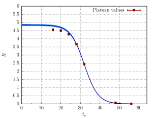
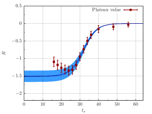
Figure 3: Plateau values plotted against the different $t_{s}$ for vanishing momentum transfer $Q^{2}=0$ for the E5 ensemble. The connected contribution (smeared-local) is shown on the left, the disconnected (smeared-smeared) on the right. A function of the form (30) has been fitted to the data.

To investigate the $t_{s}$-dependence of the ratios, we fitted constants to the plateau regions of the ratios for the different values of $t_{s}$. The plateau values obtained are plotted against $t_{s}$ in figure 3 for the E5 ensemble, which has the highest statistics of all ensembles studied so far. The blue line indicates a function of the form (30), which has been fitted to the data. Clearly, the data deviate from the expected $t_{s}$-dependence for the smaller values $t_{s}<24$ for both the connected and the disconnected contribution. However, for larger source-sink separations our data show the expected $t_{s}$-dependence. The deviation at small $t_{s}$ indicates the presence of excited state contributions for $t_{s}<24$.

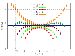
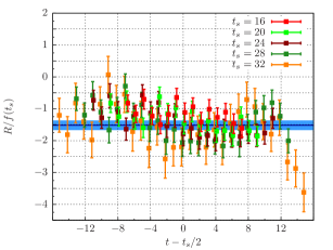
Figure 4: Results for the ratios corrected by the $t_{s}$-dependence for vanishing momentum transfer $Q^{2}=0$ for the E5 ensemble. The connected contribution (smeared-local) is shown on the left, the disconnected (smeared-smeared) on the right. The blue lines indicate the results of the global fit to a constant. The fit ranges in $t$ are listed in table 3.

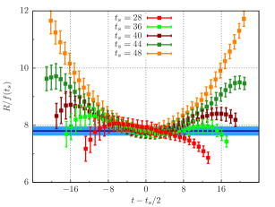
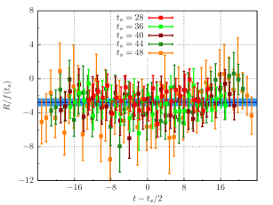
Figure 5: Same as figure 4 shown for the F7 ensemble. The fit ranges in $t$ are listed in table 3.

In figures 4 and 5 the ratios are plotted against the time $t$ of the operator insertion at each value of the sink timeslice $t_{s}$ for E5 and for F7, which has the lightest pion mass of all ensembles studied so far. To account for the $t_{s}$-dependence (cf. equation (30)) we have divided the ratios by the factor $f(t_{s})$. Provided that excited state contributions are sufficiently suppressed, one expects the quantity $R(t,t_{s},0,0)/f(t_{s})$ to form plateaus in $t$ about $t_{s}/2$, which are independent of $t_{s}$. From the plots for the E5 ensemble one can easily see that the ratios show a systematic trend as the source-sink separation $t_{s}$ is increased, which is particularly apparent in the case of the quark-connected contribution. At the same time one observes that consistent plateaus are obtained when $t_{s}\geq 24$. For the quark-disconnected part the trend is somewhat obscured by the larger statistical errors. The same $t_{s}$-behavior was already observed in the plateau values shown in figure 3. The most likely explanation is the presence of excited state contributions for $t_{s}<24$. In order to avoid a systematic bias, we have excluded ratios with $t_{s}<24$ from the subsequent analysis.

label		$t_{s}$ values in global fit
E3 - E5	connected	$24$, $28$, $32$
	disconnected	$24$, $26$, $28$, $30$, $32$
F6, F7	connected	$28$, $36$, $40$, $44$, $48$
	disconnected	$24$, $28$, $32$, $36$, $40$, $44$, $48$

Table 2: The values of $t_{s}$ that have been used in the global fits.

The blue lines in the plots of figures 4 and 5 show the results of global fits to a constant within the plateau regions, applied to the data computed for $t_{s}\geq 24$. The values of $t_{s}$, that have been used for the global fit are listed in table 2. Furthermore, in table 3 we have compiled the fit ranges in $t$ applied to the ensembles E5 and F7, which are shown in figures 4 and 5. The fit result is proportional to the unnormalized scalar form factor at vanishing momentum transfer,

$$\frac{R(t,t_{s},0,0)}{f(t_{s})}=\frac{\left<\pi(0)\right|\mathcal{O}_{\rm{S}}(0)\left|\pi(0)\right>}{2m_{\pi}}=\frac{1}{2m_{\pi}}F_{{}_{\rm S}}^{\rm bare}(Q^{2}=0)\,,$$ (31)

where the pion mass $m_{\pi}=E_{\pi}(0)$ is known from the two-point function $C_{2\textnormal{pt}}(t,0)$.

We end this discussion with the observation that our method for the evaluation of the quark-disconnected contribution can resolve the corresponding ratio with good statistical accuracy at vanishing momentum transfer. The plots on the right-hand side of figures 4 and 5, clearly show a good signal, which differs from zero within several standard deviations.

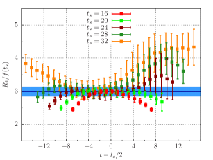
Figure 6: Results for the ratios corrected by the time-dependence for $Q^{2}=0.278$ GeV² for the E5 ensemble. The connected contribution (smeared-local) is shown on the left, the disconnected (smeared-smeared) on the right. The blue lines indicate the results of the global fit. The fit ranges in $t$ are listed in table 3.

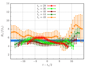
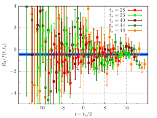
Figure 7: Same as figure 6 shown for the F7 ensemble at $Q^{2}=0.121$ GeV². The fit ranges in $t$ are listed in table 3.

V.2 Ratios for $Q^{2}\neq 0$

As was mentioned above, we cannot employ twisted boundary conditions to study the $Q^{2}$-dependence of the scalar form factor. Non-vanishing values of $Q^{2}$ are obtained by projecting the final-state pion and the insertion point of the operator onto the values of $\mathbf{p}_{f}$ and $\mathbf{q}$, respectively. On a finite lattice with spatial extent $L$ the Fourier momenta are discrete, and the smallest possible momentum is $\left|\mathbf{p}\right|=2\pi/L$. For the ensembles E5 and F7, the minimum momentum transfer corresponds to $Q^{2}=0.278$ GeV² and $Q^{2}=0.121$ GeV², respectively.

label	connected $Q^{2}=0$					disconnected $Q^{2}=0$					connected $Q_{1}^{2}$					disconnected $Q_{1}^{2}$
		$t_{s}$		$t$			$t_{s}$		$t$			$t_{s}$		$t$			$t_{s}$		$t$
E5		$24$		$5-19$			$24$		$4-20$			$24$		$7-14$			$24$		$9-21$
							$26$		$4-22$								$26$		$10-23$
		$28$		$6-22$			$28$		$5-23$			$28$		$9-15$			$28$		$10-24$
							$30$		$5-25$								$30$		$10-26$
		$32$		$12-20$			$32$		$6-26$			$32$		$10-16$			$32$		$10-27$
F7							$24$		$4-20$								$24$		$3-21$
		$28$		$6-15$			$28$		$5-23$			$28$		$6-12$			$28$		$4-25$
							$32$		$6-26$								$32$		$7-29$
		$36$		$13-28$			$36$		$7-29$			$36$		$6-13$			$36$		$12-32$
		$40$		$18-25$			$40$		$8-32$			$40$		$18-27$			$40$		$16-35$
		$44$		$18-28$			$44$		$8-36$			$44$		$18-27$			$44$		$20-39$
		$48$		$19-29$			$48$		$8-40$			$48$		$18-28$			$48$		$23-43$

Table 3: Values of the source-sink separation $t_{s}$ and the interval in $t$ used in the global fits to the connected and disconnected contributions to the E5 and F7 ensembles.

To increase statistics for quark-disconnected contributions we have again used four different source positions in the calculation of quark propagators. Additionally, we have averaged over all equivalent momenta, e.g. $(0,0,2\pi/L)$, $(0,2\pi/L,0)$ and $(2\pi/L,0,0)$ for the smallest non-zero value of $Q^{2}$.

As explained above, we use ratio $R_{1}$ of equation (27) for the analysis for the connected, and ratio $R_{3}$ of equation (28) for the disconnected contribution. Both ratios have known time-dependences which we can correct for. The ratios with the time-dependence divided out are shown in figures 6 and 7, where they are plotted against the operator insertion time $t$ for different values of $t_{s}$. Within our statistical accuracy we do not see a trend in the data computed for non-vanishing momentum transfer at different values of $t_{s}$, unlike the case of $Q^{2}=0$ discussed earlier. Nonetheless, we again exclude the data with $t_{s}<24$ from the analysis, to be sure that systematic effects from excited states are under control.

As before, the blue lines in figures 6 and 7 indicate the results from a global fit to the plateau regions for different values of $t_{s}\geq 24$. From the fit results the scalar form factor for this momentum transfer can be calculated,

$$R_{1}(t,t_{s},\mathbf{p}_{i},\mathbf{p}_{f})/f(t_{s})=\frac{\left<\pi(\mathbf{p}_{i})\right|\mathcal{O}_{\rm{S}}(0)\left|\pi(\mathbf{p}_{f})\right>}{2\sqrt{E_{\pi}(\mathbf{p}_{i})E_{\pi}(\mathbf{p}_{f})}}=\frac{1}{2\sqrt{E_{\pi}(\mathbf{p}_{i})E_{\pi}(\mathbf{p}_{f})}}\,F_{{}_{\rm S}}^{\rm bare}(Q^{2})\,,$$ (32)

$$R_{3}(t,t_{s},\mathbf{p}_{i},\mathbf{p}_{f})/f(t,t_{s})=\frac{\left<\pi(\mathbf{p}_{i})\right|\mathcal{O}_{\rm{S}}(0)\left|\pi(\mathbf{p}_{f})\right>}{2\sqrt{E_{\pi}(\mathbf{p}_{i})E_{\pi}(\mathbf{p}_{f})}}=\frac{1}{2\sqrt{E_{\pi}(\mathbf{p}_{i})E_{\pi}(\mathbf{p}_{f})}}\,F_{{}_{\rm S}}^{\rm bare}(Q^{2})\,.$$ (33)

While the relative contribution of the quark-disconnected diagram to the form factor is smaller compared to the case of vanishing momentum transfer, $Q^{2}=0$, we note that our method is clearly able to resolve a signal.

In addition, we have included data for another momentum transfer, where the final state of the pion is projected to $\left|\mathbf{p}_{f}\right|=2\cdot 2\pi/L$. The corresponding pion two-point functions $C_{2\textrm{pt}}(t_{s},\mathbf{p}_{f})$, which occur in the ratios, are fluctuating strongly, especially for larger values of $t_{s}\lesssim T/2$, such that a reliable estimate for the form factor is not possible using the two-point data themselves. Instead of dividing the three-point function by $C_{2\textnormal{pt}}(t_{s},\mathbf{p}_{f})$ we use the fitted two-point function in order to compute the ratios $R_{1}$ and $R_{3}$, which reduces their statistical fluctuations.

V.3 The $Q^{2}$ dependence of the form factor

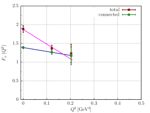
Figure 8: The $Q^{2}$-dependence of the scalar form factor: on the left-hand side E5 with a pion mass of $455$ MeV, on the right-hand side F7 with $m_{\pi}=280$ MeV. The red points show the results for the total form factor and the green points for the connected contribution only.

We briefly recall the definition of the scalar radius in terms of the scalar form factor

$$\left\langle r^{2}\right\rangle^{\pi}_{{}_{\rm S}}=-\frac{6}{F^{\pi}_{{}_{\rm S}}(0)}\frac{\partial F^{\pi}_{{}_{\rm S}}(Q^{2})}{\partial Q^{2}}\Big{|}_{Q^{2}=0}\,.$$ (34)

The scalar form factor admits an expansion, which has the general form

$$F^{\pi}_{{}_{\rm S}}\left(Q^{2}\right)=F^{\pi}_{{}_{\rm S}}(0)\left(1-\frac{1}{6}\left\langle r^{2}\right\rangle^{\pi}_{{}_{\rm S}}Q^{2}+\mathcal{O}(Q^{4})\right)\,,$$ (35)

and which is consistent with the definition (34) of the scalar radius.

In practice, the slope at $Q^{2}=0$ is difficult to determine on the lattice in a model-independent way. Usually one fits the lattice data for form factors obtained at a few discrete values of $Q^{2}$ to some phenomenological model such as vector meson dominance. In the case of the pion vector form factor, which is amenable to the use of twisted boundary conditions, it is possible to tune $Q^{2}$ so as to generate a high density of data points in the immediate vicinity of $Q^{2}=0$ from which the slope can be extracted without any model assumptions Brandt:2013dua .

Here we must resort to a more naive treatment, since twisted boundary conditions cannot be used to evaluate the quark-disconnected contribution, so that the resolution in $Q^{2}$ is only quite rough. As a consequence, we estimate the scalar radius from a linear fit over a relatively broad interval in $Q^{2}$, using three data points only. However, we compare different fit ansätze in an attempt to investigate the systematics of this procedure.

In figure 8 we show the $Q^{2}$-dependence for the ensembles E5 and F7. Both plots show the total form factor and the results obtained when the disconnected contributions are neglected. According to (35) a linear function was fitted to the data to estimate the scalar radius. For both ensembles shown here the descending slope of the linear curves is clearly steeper for the total form factor than for the connected part only. This stresses the importance of including the disconnected diagram for determining the scalar radius.

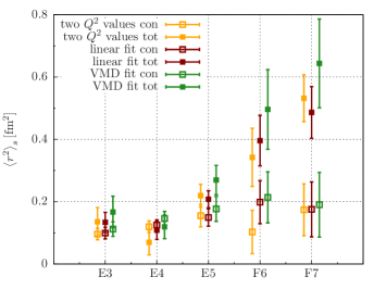
Figure 9: A comparison of different descriptions of the form factor data: a linear interpolation (yellow) at the two smallest values of $Q^{2}$, and both a linear (red) and a VMD-inspired (green) fit to the three smallest values of $Q^{2}$, with the radii resulting from considering only the connected part and the complete three-point function shown using open and filled symbols, respectively.

		$F^{\pi}_{{}_{\rm S}}\left(0\right)$	$Q_{1}^{2}\left[\textnormal{GeV}^{2}\right]$	$F^{\pi}_{{}_{\rm S}}\left(Q_{1}^{2}\right)$	$Q_{2}^{2}\left[\textnormal{GeV}^{2}\right]$	$F^{\pi}_{{}_{\rm S}}\left(Q_{2}^{2}\right)$	$\left\langle r^{2}\right\rangle^{\pi}_{{}_{\rm S}}\left[\textnormal{fm}^{2}\right]$
E3	connected	$1.39\pm 0.01$	$0.319$	$1.20\pm 0.03$	$0.565$	$1.02\pm 0.12$	$0.099\pm 0.018$
	total	$1.97\pm 0.11$		$1.61\pm 0.07$		$1.33\pm 0.14$	$0.134\pm 0.032$
E4	connected	$1.39\pm 0.01$	$0.311$	$1.17\pm 0.04$	$0.548$	$0.93\pm 0.11$	$0.125\pm 0.017$
	total	$1.88\pm 0.09$		$1.70\pm 0.06$		$1.38\pm 0.13$	$0.208\pm 0.027$
E5	connected	$1.36\pm 0.01$	$0.278$	$1.11\pm 0.05$	$0.471$	$1.02\pm 0.19$	$0.149\pm 0.028$
	total	$1.82\pm 0.05$		$1.34\pm 0.06$		$1.17\pm 0.20$	$0.208\pm 0.027$
F6	connected	$1.44\pm 0.03$	$0.128$	$1.36\pm 0.07$	$0.221$	$1.02\pm 0.14$	$0.197\pm 0.069$
	total	$1.97\pm 0.10$		$1.60\pm 0.08$		$1.17\pm 0.16$	$0.396\pm 0.081$
F7	connected	$1.39\pm 0.03$	$0.121$	$1.26\pm 0.06$	$0.203$	$1.17\pm 0.23$	$0.175\pm 0.088$
	total	$1.88\pm 0.09$		$1.37\pm 0.08$		$1.23\pm 0.24$	$0.487\pm 0.083$

Table 4: Numerical results of the scalar pion form factor $F^{\pi}_{{}_{\rm S}}\left(Q^{2}\right)$ for three different momentum transfers $Q^{2}$ and the results for the scalar radius $\left\langle r^{2}\right\rangle^{\pi}_{{}_{\rm S}}$ as determined from an uncorrelated linear fit.

For all ensembles studied so far, we find the results for the three different $Q^{2}$ to be consistent with a linear $Q^{2}$ dependence within their statistical errors. In order to investigate the systematic effect in the determination of the scalar radius arising from the ansatz for the $Q^{2}$ dependence, we have compared the linear fit to a VMD-inspired fit of the form $1/(1+Q^{2}/M^{2})^{2}$ as well as a linear interpolation using only the two smallest $Q^{2}$ values. As can be inferred from figure 9 no statistically significant effect in the determination of $\left\langle r^{2}\right\rangle^{\pi}_{{}_{\rm S}}$ arising from the use of different ansätze is observed. This indicates that any possible curvature contained in the data cannot be resolved at the current level of statistical accuracy.

We choose the linear fit as a reasonable compromise between achieving a well-motivated description of the data and keeping the statistical error of the fitted radius in check. The results for the form factor and the scalar radius from the linear fit are summarized in table 4.

V.4 Chiral extrapolation

Since our simulations of the scalar radius have been performed with pion masses larger than the physical mass $m_{\pi}>m_{\pi,\textnormal{phys}}$, we have to perform a chiral extrapolation. In chiral perturbation theory at NLO the scalar radius of the pion is Gasser:1983yg ; Gasser:1990bv ; Bijnens:1998fm

$$\left\langle r^{2}\right\rangle^{\pi}_{{}_{\rm S}}=\frac{1}{(4\pi F)^{2}}\left(-\frac{13}{2}\right)+\frac{6}{(4\pi F)^{2}}\left[\overline{\ell}_{4}+\ln\left(\frac{m_{\pi,phys}^{2}}{m_{\pi}^{2}}\right)\right]$$ (36)

where $F=92.2$ MeV PDG:2012 is the pion decay constant.

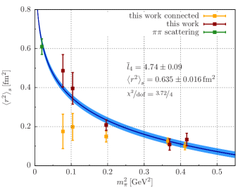
Figure 10: The $m_{\pi}^{2}$-dependence of the scalar radius. The blue band is a fit to the lattice data obtained from both quark-connected and -disconnected diagrams.

In figure 10 the values obtained for $\left\langle r^{2}\right\rangle^{\pi}_{{}_{\rm S}}$ are plotted against the square of the pion mass, $m_{\pi}^{2}$. The point shown at the physical pion mass is the value obtained from $\pi\pi$-scattering Colangelo:2001df . The expression (36) from NLO $\chi$PT has been fitted to the data and the obtained curve is shown in blue. This fit allows a determination of the low energy constant $\overline{\ell}_{4}$ for which we find $\overline{\ell}_{4}=4.74\pm 0.09$, where the error is only statistical.

This is in excellent agreement with the result of ref. Brandt:2013dua , which was extracted from chiral fits to the pseudoscalar decay constant computed on the CLS ensembles at three different lattice spacings. The result for the scalar radius at physical pion mass obtained from our NLO fit is

$$\left\langle r^{2}\right\rangle^{\pi}_{{}_{\rm S}}=0.635\pm 0.016\ \textnormal{fm}^{2}\,,$$ (37)

which agrees very well with the $\pi\pi$-scattering value $\left\langle r^{2}\right\rangle^{\pi}_{{}_{\rm S}}=0.61\pm 0.04$ fm² reported in ref. Colangelo:2001df . In figure 10 one can see that our data are well described by $\chi$PT at NLO. As already indicated in figure 8, the quark-disconnected contribution to the scalar radius of the pion is not negligible. The yellow points in figure 10 show the data obtained from the connected contribution only. For the ensembles analyzed so far, we find that the disconnected contribution to the scalar radius becomes more important as the pion mass approaches its physical value. Clearly, neglecting the disconnected diagram fails to reproduce the phenomenological expectation for the scalar radius.

These findings differ from the results obtained by the JLQCD and TWQCD collaborations Aoki:2009qn , where no significant pion mass dependence of the scalar radius was observed. The reason for this discrepancy is presently unknown. Here we only comment that the two simulations in question differ substantially regarding the value of the lattice spacing, the minimum value of $m_{\pi}L$, and the type of fermionic discretization. It should also be noted that the contribution of quark-disconnected diagrams in Aoki:2009qn , though significant, was observed to be much smaller than in our study. Clearly, more work is needed to investigate the systematics of these calculations. To this end we will add more ensembles at smaller pion masses and different lattice spacings.

VI Conclusions

The combination of the hopping parameter expansion with the use of stochastic sources provides a powerful means for estimating quark-disconnected contributions to hadronic form factors. We have been able to obtain a clearly non-vanishing signal for the scalar form factor of the pion both at $Q^{2}=0$ (where there is a large subtraction of the vacuum contribution) and at non-vanishing momentum transfer, where the correlation functions become intrinsically noisy.

We find that the disconnected contribution to the scalar form factor is not negligible, and that indeed the purely connected part of the form factor fails to reproduce the expected logarithmic behaviour of the pion scalar radius as a function of the pion mass. This is in qualitative agreement with what has been found in partially quenched $\chi$PT Juttner:2011ur . From our determination of the pion scalar radius, we can derive a lattice estimate of the low-energy constant $\overline{\ell}_{4}=4.74\pm 0.09$, which is in fair agreement with the phenomenological estimate Colangelo:2001df $\bar{\ell}_{4}=4.4\pm 0.2$ based on the analysis of $\pi\pi$-scattering amplitudes.

The present study is based on a single, albeit rather fine, lattice spacing. It is therefore important to repeat this study on ensembles with different values of the lattice spacing, to estimate the size of discretization effects and perform an extrapolation to the continuum limit. Another potential source of systematic errors are finite-volume effects. While all of our lattices satisfy $M_{\pi}L\geq 4$, it is desirable to include further, even larger, lattice volumes to ensure that finite-volume effects are indeed fully under control.

Another source of systematic error in the determination of the pion scalar radius, and hence of $\bar{\ell}_{4}$, is the simple linear fit used to estimate the derivative of the scalar form factor at vanishing $Q^{2}$. It would be highly desirable to augment this somewhat naive approximation by using partially twisted boundary conditions for the connected part along the lines of Jiang:2006gna ; Brandt:2013mb . Unfortunately this method is fundamentally inapplicable to the disconnected part, where the same quark propagator connects to the operator insertion on both sides, and some interpolation will necessarily be required in this case. However, all our data are consistent with a linear $Q^{2}$ dependence, and any possible curvature cannot be resolved with our current accuracy.

Finally, another potential for systematic error lies in the use of NLO $\chi$PT formulae, which may not always give a good description of pion form factors Brandt:2013dua . The ability of the NLO expressions to describe the numerical data crucially depends on the overall accuracy of the latter. If the the statistical errors in the determinations of the scalar form factor and radius can be substantially decreased, one may have to resort to $\chi$PT at NNLO.

- (1) J. Gasser and H. Leutwyler, Annals Phys. 158, 142 (1984).
- (2) J. Gasser and H. Leutwyler, Nucl. Phys. B250, 465 (1985).
- (3) S. Dürr et al., JHEP 1108, 148 (2011), [1011.2711].
- (4) S. Dürr et al., Phys. Lett. B701, 265 (2011), [1011.2403].
- (5) PACS-CS Collaboration, S. Aoki et al., Phys. Rev. D81, 074503 (2010), [0911.2561].
- (6) ALPHA Collaboration, J. Heitger, R. Sommer and H. Wittig, Nucl. Phys. B588, 377 (2000), [hep-lat/0006026].
- (7) L. Giusti, P. Hernandez, M. Laine, P. Weisz and H. Wittig, JHEP 0401, 003 (2004), [hep-lat/0312012].
- (8) L. Giusti, P. Hernandez, M. Laine, P. Weisz and H. Wittig, JHEP 0404, 013 (2004), [hep-lat/0402002].
- (9) Bern-Graz-Regensburg (BGR) Collaboration, C. Gattringer, P. Huber and C. Lang, Phys. Rev. D72, 094510 (2005), [hep-lat/0509003].
- (10) A. Hasenfratz, R. Hoffmann and S. Schaefer, Phys. Rev. D78, 054511 (2008), [0806.4586].
- (11) S. Beane et al., Phys. Rev. D86, 094509 (2012), [1108.1380].
- (12) F. Bernardoni, J. Bulava and R. Sommer, PoS LATTICE2011, 095 (2011), [1111.4351].
- (13) P. Damgaard, U. Heller and K. Splittorff, Phys. Rev. D86, 094502 (2012), [1206.4786].
- (14) S. Borsanyi et al., Phys.Rev. D88, 014513 (2013), [1205.0788].
- (15) G. Herdoiza, K. Jansen, C. Michael, K. Ottnad and C. Urbach, JHEP 1305, 038 (2013), [1303.3516].
- (16) Bern-Graz-Regensburg (BGR) Collaboration, S. Capitani, C. Gattringer and C. Lang, Phys. Rev. D73, 034505 (2006), [hep-lat/0511040].
- (17) QCDSF/UKQCD Collaboration, D. Brömmel et al., Eur. Phys. J. C51, 335 (2007), [hep-lat/0608021].
- (18) F.-J. Jiang and B. Tiburzi, Phys. Lett. B645, 314 (2007), [hep-lat/0610103].
- (19) JLQCD Collaboration, T. Kaneko et al., PoS LAT2007, 148 (2007), [0710.2390].
- (20) C. Alexandrou and G. Koutsou, PoS LAT2007, 150 (2007), [0710.2441].
- (21) P. Boyle et al., JHEP 0807, 112 (2008), [0804.3971].
- (22) JLQCD and TWQCD Collaborations, S. Aoki et al., Phys. Rev. D80, 034508 (2009), [0905.2465].
- (23) O. H. Nguyen, K.-I. Ishikawa, A. Ukawa and N. Ukita, JHEP 1104, 122 (2011), [1102.3652].
- (24) JLQCD Collaboration, H. Fukaya et al., PoS LATTICE2012, 198 (2012), [1211.0743].
- (25) B. B. Brandt, A. Jüttner and H. Wittig, PoS ConfinementX, 112 (2012), [1301.3513].
- (26) J. Gasser and H. Leutwyler, Phys. Lett. B125, 325 (1983).
- (27) J. F. Donoghue, J. Gasser and H. Leutwyler, Nucl. Phys. B343, 341 (1990).
- (28) J. Gasser and U. G. Meissner, Nucl. Phys. B357, 90 (1991).
- (29) B. Moussallam, Eur. Phys. J. C14, 111 (2000), [hep-ph/9909292].
- (30) G. Colangelo, J. Gasser and H. Leutwyler, Nucl. Phys. B603, 125 (2001), [hep-ph/0103088].
- (31) A. Jüttner, JHEP 1201, 007 (2012), [1110.4859].
- (32) A. Jüttner, PoS LATTICE2012, 196 (2012), [1212.2559].
- (33) K. Bitar, A. Kennedy, R. Horsley, S. Meyer and P. Rossi, Nucl. Phys. B313, 348 (1989).
- (34) H. Neff, N. Eicker, T. Lippert, J. W. Negele and K. Schilling, Phys. Rev. D64, 114509 (2001), [hep-lat/0106016].
- (35) SESAM Collaboration, G. S. Bali, H. Neff, T. Duessel, T. Lippert and K. Schilling, Phys. Rev. D71, 114513 (2005), [hep-lat/0505012].
- (36) C. Thron, S. Dong, K. Liu and H. Ying, Phys. Rev. D57, 1642 (1998), [hep-lat/9707001].
- (37) S. Collins, G. Bali and A. Schäfer, PoS LAT2007, 141 (2007), [0709.3217].
- (38) V. Gülpers, G. von Hippel and H. Wittig, PoS LATTICE2012, 181 (2012).
- (39) B. Sheikholeslami and R. Wohlert, Nucl. Phys. B259, 572 (1985).
- (40) M. Lüscher, S. Sint, R. Sommer and P. Weisz, Nucl. Phys. B478, 365 (1996), [hep-lat/9605038].
- (41) M. Lüscher, Comput.Phys.Commun. 165, 199 (2005), [hep-lat/0409106].
- (42) M. Lüscher, JHEP 0712, 011 (2007), [0710.5417].
- (43) ALPHA Collaboration, K. Jansen and R. Sommer, Nucl. Phys. B530, 185 (1998), [hep-lat/9803017].
- (44) S. Capitani, M. Della Morte, G. von Hippel, B. Knippschild and H. Wittig, PoS LATTICE2011, 145 (2011), [1110.6365].
- (45) P. Fritzsch et al., Nucl. Phys. B865, 397 (2012), [1205.5380].
- (46) G. Martinelli and C. T. Sachrajda, Nucl. Phys. B316, 355 (1989).
- (47) G. S. Bali, S. Collins and A. Schäfer, Comput.Phys.Commun. 181, 1570 (2010), [0910.3970].
- (48) V. Gülpers, Diploma thesis, JGU Mainz, 2011, URL: http://wwwkph.kph.uni-mainz.de/T//pub/diploma/Dipl_Th_Guelpers.pdf.
- (49) P. Boyle, J. Flynn, A. Jüttner, C. Sachrajda and J. Zanotti, JHEP 0705, 016 (2007), [hep-lat/0703005].
- (50) LHP Collaboration, F. D. Bonnet, R. G. Edwards, G. T. Fleming, R. Lewis and D. G. Richards, Phys. Rev. D72, 054506 (2005), [hep-lat/0411028].
- (51) S. Güsken et al., Phys. Lett. B227, 266 (1989).
- (52) C. Alexandrou, F. Jegerlehner, S. Güsken, K. Schilling and R. Sommer, Phys. Lett. B256, 60 (1991).
- (53) UKQCD Collaboration, C. Allton et al., Phys. Rev. D47, 5128 (1993), [hep-lat/9303009].
- (54) P. F. Bedaque, Phys.Lett. B593, 82 (2004), [nucl-th/0402051].
- (55) C. Sachrajda and G. Villadoro, Phys.Lett. B609, 73 (2005), [hep-lat/0411033].
- (56) UKQCD, J. Flynn, A. Jüttner and C. Sachrajda, Phys.Lett. B632, 313 (2006), [hep-lat/0506016].
- (57) G. de Divitiis, R. Petronzio and N. Tantalo, Phys.Lett. B595, 408 (2004), [hep-lat/0405002].
- (58) B. B. Brandt, A. Jüttner and H. Wittig, JHEP 1311, 034 (2013), [1306.2916].
- (59) J. Bijnens, G. Colangelo and P. Talavera, JHEP 9805, 014 (1998), [hep-ph/9805389].
- (60) Particle Data Group, J. Beringer et al., Phys. Rev. D86, 010001 (2012).