Laser assisted Compton scattering of X-ray photons

Abstract

The Compton scattering of X-ray photons, assisted by a short intense optical laser pulse, is discussed. The differential scattering cross section reveals the interesting feature that the main Klein-Nishina line is accompanied by a series of side-lines forming a broad plateau where up to ${\cal O}(10^{3})$ laser photons participate simultaneously in a single scattering event. An analytic formula for the width of the plateau is given. Due to the non-linear mixing of X-ray and laser photons a frequency dependent rotation of the polarization of the final state X-ray photons relative to the scattering plane emerges. A consistent description of the scattering process with short laser pulses requires to work with X-ray pulses. An experimental investigation can be accomplished, e.g., at LCLS or the European XFEL in the near future.

I Introduction

Compton scattering Compton (1923), i.e. the scattering of X or $\gamma$ rays off free electrons is one of the fundamental interaction processes of photons with charged particles. A particular feature is the dependence of the frequency $\omega_{\rm KN}^{\prime}$ of the scattered photon on the angle $\vartheta$, $\omega_{\rm KN}^{\prime}=\omega_{X}/(1+\frac{\omega_{X}}{m}[1-\cos\vartheta])$, in the initial rest frame of the scattering particle with mass $m$. For linearly polarized X-rays the scattered photon polarization direction is the same as for electric dipole radiation. These properties become modified in laser assisted Compton scattering $X+L+e\to e^{\prime}+X^{\prime}$, where we suppose alignment of the X-ray beam ($X$, frequency $\omega_{X}\sim\mathcal{O}(\mathrm{k}\mathrm{eV})$) and an intense optical laser pulse ($L$, frequency $\omega_{L}\sim\mathcal{O}(\mathrm{eV})$). The frequency $\omega^{\prime}$ of the scattered photon $X^{\prime}$ in the initial rest frame of the electron $e$ reads (with $\hbar=c=1$)

$$\omega^{\prime}(\ell,\vartheta) =\frac{\omega_{X}+\ell\omega_{L}}{1+\frac{\omega_{X}+\ell\omega_{L}}{m}(1-\cos\vartheta)}\,.$$ (1)

That means a non-linear frequency mixing occurs with $\ell$ parametrizing the amount of energy and momentum absorbed from the laser field in the scattering process. The quantity $\ell$ can be related to the number of involved laser photons, in particular in the limit of infinite monochromatic plane waves, where the values of $\ell$ become discrete $\ell_{N}$, with integers $N$ referring to the number of exchanged laser photons (see Appendix A for details). The value of $\ell$ may be positive or negative, leading to the formation of side-bands in the energy spectrum Ehlotzky (1987). A similar effect has been observed also for laser assisted atomic processes Weingartshofer et al. (1977); Taïeb et al. (2008). Obviously, $\ell=0$ recovers the laser-free scattering of an X-ray photon with known Klein-Nishina (KN) kinematics. A large frequency ratio $\varkappa=\omega_{X}/\omega_{L}$ leads to a strong dynamical enhancement of non-linear multi-laser photon effects such that many side-lines form a broad plateau reaching to $|\ell|\gg 1$. Although the possibility of a strong enhancement was recognized in Ehlotzky (1987), the shape of the spectrum in frequency space and the cut-off values of $\ell$, in particular their angular dependencies, have never been calculated precisely to the best of our knowledge. This gap will be filled in this paper, where we calculate the frequency spectrum and provide a formula for the angular dependence of the cut-off energies of the side-band plateau.

Observing the plateau of side-lines within a certain frequency interval determined by cut-off values with special angular dependencies is a clear experimental signal for laser assisted Compton scattering of X-rays, i.e. a new possibility to observe ${\cal O}(10^{3})$ multi-photon effects in strong-field QED. In addition, as we shall show below, the polarization properties of $X^{\prime}$ represent a new feature. The non-linear frequency mixing leads to a frequency dependent rotation of the polarization of the final state photons. This rotation does not affect the main KN line ($\ell=0$) and is useful to identify the side-bands in an experiment.

The basic scattering process can be understood qualitatively in a classical picture, where the “slow” electron motion due to the laser is described classically. For high-intensity laser fields of the order of $10^{18}\text{\,}\mathrm{W}\mathrm{/}\mathrm{c}\mathrm{m}^{2}$ the motion of electrons becomes relativistic and non-linear, resembling a figure-8 motion with a velocity component in the laser beam direction Sarachik and Schappert (1970); Di Piazza et al. (2012), superimposed to the usual transverse motion. In this picture, laser assisted Compton scattering corresponds to the scattering of X-rays off accelerated charges, and the broadening of the KN line occurs due to a time dependent Doppler shift induced by the figure-8 motion.

In our approach we fully take into account the finite lengths of both the X-ray and laser pulses, going beyond infinite monochromatic plane wave approximation Oleĭnik (1968); Guccione-Gush and Gush (1975); Akhiezer and Merenkov (1985); Ehlotzky (1987); Puntajer and Leubner (1989); Ehlotzky (1989); Zhukovskii and Nikitina (1973); Baier et al. (1998) or the limit of long laser pulses and infinite X-ray waves Nedoreshta et al. (2013a). Pulse shape effects have been recently proved to have a significant impact of the scattering spectra in non-linear Compton scattering Narozhnyi and Fofanov (1996); Boca and Florescu (2009); Heinzl et al. (2010a); Seipt and Kämpfer (2011); Mackenroth and Di Piazza (2011); Krajewska and Kamiński (2012a); Seipt and Kämpfer (2013), pair production Heinzl et al. (2010b); Nousch et al. (2012); Krajewska et al. (2013); Kohlfürst et al. (2013) and other strong field QED processes Ilderton et al. (2011); Di Piazza et al. (2012).

Taking into account the finite pulse length is necessary as we envisage a specific experimental set-up involving a petawatt class optical laser in combination with an X-ray free electron laser, which both produce short femtosecond light pulses. In some previous papers, relations for the cross section were calculated either for small numbers of exchanged laser photons $N$ Oleĭnik (1968); Guccione-Gush and Gush (1975); Akhiezer and Merenkov (1985), or they were limited to non-relativistic intensities Ehlotzky (1987), or were restricted to the discussion of energy-integrated angular distributions Puntajer and Leubner (1989); the partial cross sections have been calculated for arbitrary values of $N$ in terms of generalized Bessel functions, e.g. in Ehlotzky (1989).

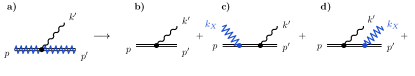
Figure 1: (Color online) Expansion of the Feynman diagram (a) for photon emission off a dressed electron (double zig-zag line: electron in the combined laser and X-ray field, plain double line: electron in the laser background, wavy line: photon, and zig-zag line: X-ray) for a weak X-ray field in powers of $a_{X}$, yielding spontaneous emission (b), laser assisted Compton scattering (c) and induced emission (d).

Our paper is organised as follows: In Section II we formulate the matrix element for photon emission in the combined X-ray and laser fields and discuss the physical significance of the various terms occurring in a weak field expansion in the X-ray field. In Section III the leading order contribution in the X-ray field is evaluated and used to calculate an expression for the cross section for laser assisted Compton scattering. The essential properties of the photon spectrum are discussed in Section IV where we present results for the differential cross section as well as the final photon polarization for a representative set of parameters. High order multi-photon effects are quantified via an analytic formula for the cut-off values of the frequency spectrum. We discuss and summarize our results in Section V where we also address some aspects of an experimental realization. Appendix A provides a brief discussion on the limit of infinitely long plane waves.

II Matrix Element

We describe the photon beams as a classical plane wave background field with four-vector potential $A^{\mu}=A^{\mu}_{X}(\varkappa\phi)+A^{\mu}_{L}(\phi)$, defining $\phi=k_{L}\cdot x\equiv k_{L}^{\mu}x_{\mu}$ with $k_{L}^{\mu}=(\omega_{L},\mathbf{k}_{L})$ and $k_{X}^{\mu}=\varkappa k_{L}^{\mu}$. We consider orthogonal linear polarizations, $A_{X}\cdot A_{L}=0$. The vector potentials are parametrized as $A_{j}^{\mu}(\phi)=\frac{ma_{j}}{e}\epsilon_{j}^{\mu}g_{j}(\phi)\cos\phi$, $j\in\{X,L\}$, with the modulus of the electron charge $e$, normalized polarization vectors $\epsilon_{j}^{\mu}$ and invariant laser strength parameters $a_{j}$. We emphasize the appearance of the envelope functions $g_{j}$ accounting for the finite pulse lengths $T_{j}$ of both the X-ray and the laser pulses which are assumed to be synchronized temporally.

For the given background field $A^{\mu}$ we may work in the Furry picture employing Volkov states Volkov (1935); Di Piazza et al. (2012)

$$\Psi_{p}(x,A) =e^{-ip\cdot x-\frac{i}{2k_{L}\cdot p}\int\limits^{\phi}{\mathrm{d}}\phi^{\prime}[2ep\cdot A(\phi^{\prime})-e^{2}A^{2}(\phi^{\prime})]}$$

$$\qquad\times\left(1+\frac{e\not{k}_{L}\not{A}}{2k_{L}\cdot p}\right)u_{p}\,,$$ (2)

as non-perturbative solutions of the Dirac equation $(i\not{\partial}-e\not{A}-m)\Psi_{p}(x)=0$. The free Dirac spinors $u_{p}$ fulfil $(\not{p}-m)u_{p}=0$ and are normalized to $\mathrm{bar}u_{p}u_{p}=2m$. Moreover, Feynman’s slash notation $\not{p}=\gamma_{\mu}p^{\mu}$ is employed.

The $S$ matrix for the emission of the photon $X^{\prime}$ with momentum $k^{\prime}$ is given by

$$S =-ie\int\!{\mathrm{d}}^{4}x\,\mathrm{bar}\Psi_{p^{\prime}}(x,A)\not{\epsilon}^{\prime}e^{ik^{\prime}\cdot x}\Psi_{p}(x,A)\,,$$ (3)

as depicted in Fig. 1(a). The non-perturbative expression (3), in both $a_{X}$ and $a_{L}$, is correct for arbitrary X-ray and laser intensities, describing multi-photon processes for both the laser and X-ray field. For instance, in the papers Guccione-Gush and Gush (1975); Voroshilo and Roshchupkin (1996); Krajewska and Kamiński (2012b); Augustin and Müller (2013); Voroshilo et al. (2013) situations have been discussed where it is necessary to treat both field on equal footing. However, even for present XFEL technology $a_{X}\ll 1$, and we may expand the $S$ matrix into a power series in $a_{X}$ to get

$$S=S_{0}+a_{X}(S_{+1}+S_{-1})+\mathcal{O}(a_{X}^{2})\,.$$ (4)

This corresponds to treating the field $A_{X}$ as a perturbation, going to a single X-ray photon approximation. A similar technique of expanding a Volkov wavefunction in a weak field has also been used, e.g. in Herrmann and Zhukovskii (1972); Zhukovskii and Nikitina (1973); Baier et al. (1998); Hu and Müller (2011). Here, we first discuss the physical implications of that expansion and give an interpretation for the individual terms of Eq. (4). Details of the derivation are presented in the next section.

The lowest order term $S_{0}\propto a_{X}^{0}$ (see Fig. 1(b)) corresponds to non-linear optical-laser Compton scattering without any participation of X-ray photon . This scattering of laser photons off free electrons is named commonly non-linear Thomson or Compton scattering, see e.g. Brown and Kibble (1964); Narozhnyi et al. (1965); Narozhnyi and Fofanov (1996); Harvey et al. (2009); Boca and Florescu (2009); Heinzl et al. (2010a); Seipt and Kämpfer (2011); Mackenroth and Di Piazza (2011). In the classical picture, this is the radiation due to the accelerated figure-8 motion of the electron in the laser. In the present context it may be dubbed spontaneous emission. Using moderately strong laser pulses with $a_{L}\sim 1$, the non-linear interaction with more than one photon has been verified experimentally Englert and Rinehart (1983); Bula et al. (1996); Chen et al. (1998) via the observation of harmonic radiation. In these experiments, only a rather small number of $\mathcal{O}(2\ldots 5)$ laser photons was participating in a single scattering event.

The leading order process involving X-ray photons is proportional to $a_{X}^{1}$ and consists of two terms which correspond to the absorption ($S_{+1}$, Fig. 1(c)) or the emission ($S_{-1}$, Fig. 1(d)) of a single X-ray photon from or to the initial beam. The laser assisted Compton scattering is described by $S_{+1}$ with the formal energy-momentum conservation

$$p+k_{X}+\ell k_{L}=p^{\prime}+k^{\prime}\,,$$ (5)

which arises upon the integration in (3) together with introducing the auxiliary variable $\ell$; note that one still has to integrate over $\ell$, therefore (5) has only three independent conservation laws for the light-front components Boca and Florescu (2009); Mackenroth and Di Piazza (2011)

$$\mathbf{p}^{\perp} =\mathbf{p}^{\prime\perp}+\mathbf{k}^{\prime\perp}\,, p^{-} =p^{\prime-}+k^{\prime-}\,.$$ (6)

The light-front is defined with respect to $k_{L}$ such that $k_{L}^{+}=2\omega_{L}$ is the only non-vanishing light-front component of $k_{L}$ and $\phi=\omega_{L}x^{-}$ becomes the light-front time-evolution parameter. By adopting a coordinate system in which the laser propagates in the $z$-direction the light-front components of any four-vector read $x^{\pm}=x^{0}\pm x^{3}$ and $\mathbf{x}^{\perp}=(x^{1},x^{2})^{T}$.

The fourth condition in (5), $p^{+}+k_{X}^{+}+\ell k_{L}^{+}=p^{\prime+}+k^{\prime+}$, furnishes a relation between the frequency $\omega^{\prime}$ and the variable $\ell$ via Eq. (1). This may also be turned around expressing $\ell$ as a function of $k^{\prime}$ via

$$\ell(\omega^{\prime},\vartheta)=\frac{k^{\prime}\cdot p-k_{X}\cdot(p-k^{\prime})}{k_{L}\cdot(p-k^{\prime})}\,.$$ (7)

Thus, one can chose any of the two quantities $\omega^{\prime}$ or $\ell$ to be the independent variable defining the other one. The lower limit of $\ell$ is determined by the condition $\omega^{\prime}\geq 0$, yielding $\ell\geq-\varkappa$.

The meaning of $\ell$ is that it parametrizes the amount of laser four-momentum $k_{L}$ absorbed in the scattering process and it is the Fourier conjugate to the laser phase $\phi$ Heinzl et al. (2010b); Harvey et al. (2012). It can be considered as a continuous analogue of the photon number encountered for infinite monochromatic plane wave fields Ilderton (2011); Harvey et al. (2012), cf. also Appendix A.

Due to the large frequency ratio the two partial processes (b) and (c) are separated kinematically: While photons from spontaneous emission $S_{0}$ have typical energies of $\omega^{\prime}=\mathcal{O}(\mathrm{eV})$ (Eq. (1) with $\omega_{X}=0$), the photons from laser assisted Compton scattering $S_{+1}$ are $\omega^{\prime}=\mathcal{O}(\mathrm{k}\mathrm{eV})$. The induced process $S_{-1}$, related to double Compton scattering Lötstedt and Jentschura (2009); Seipt and Kämpfer (2012); Mackenroth and Di Piazza (2013), is strongly suppressed here in the $\mathrm{k}\mathrm{eV}$ frequency range due to the large value of $\varkappa$.

III Cross Section for Laser Assisted Compton Scattering

Here we present the derivation of the matrix element for laser assisted Compton scattering $S_{+1}$ which is needed to calculate the corresponding cross section. To this end we have to linearise expression (3) in $a_{X}$ and extract the part representing the absorption of an X-ray photon from the field $A_{X}$, i.e. a process with the formal energy momentum conservation (5). For these purposes it is convenient to split the integrand of $S$ in Eq. (3) into the pre-exponential term $\Gamma(x)=(1+\frac{e\not{A}\not{k}_{L}}{2k_{L}\cdot p^{\prime}})\not{\epsilon}^{\prime}(1+\frac{e\not{k}_{L}\not{A}}{2k_{L}\cdot p})$ and a phase factor $F(x)=(p^{\prime}+k^{\prime}-p)\cdot x-\int\!{\mathrm{d}}\phi\,(\frac{ep\cdot A(\phi)}{k_{L}\cdot p}-\frac{ep^{\prime}\cdot A(\phi)}{k_{L}\cdot p^{\prime}})+(\frac{e^{2}}{2k_{L}\cdot p}-\frac{e^{2}}{2k_{L}\cdot p^{\prime}})\int\!{\mathrm{d}}\phi\,A^{2}(\phi)$, such that

$$S =-ie\int\!{\mathrm{d}}^{4}x\,\mathrm{bar}u_{p^{\prime}}\Gamma(x)u_{p}e^{iF(x)}\,,$$ (8)

where terms proportional to $a_{X}^{2}$ both in the exponent $F$ and the pre-exponential $\Gamma$ can be dropped by virtue of $a_{X}\ll 1$. We need to linearise furthermore the phase exponent according to

$$e^{iF}\approx e^{iF_{0}+iF_{X}}\approx e^{iF_{0}}(1+iF_{X})\,,$$ (9)

where $F_{0}$ is the part of the phase of $S$ independent of $A_{X}$, i.e. $\propto a_{X}^{0}$, and

$$F_{X} =\alpha_{X}\int\!{\mathrm{d}}(\varkappa\phi)\,g_{X}(\varkappa\phi)\cos(\varkappa\phi)$$ (10)

is linear in $a_{X}$ with

$$\alpha_{X} =ma_{X}\left(\frac{\epsilon_{X}\cdot p^{\prime}}{k_{X}\cdot p^{\prime}}-\frac{\epsilon_{X}\cdot p}{k_{X}\cdot p}\right)\,.$$ (11)

Multiplying with the pre-exponential we obtain up to linear order in $a_{X}$

$$\Gamma e^{iF} \approx\Gamma_{0}e^{iF_{0}}+(\Gamma_{X}+iF_{X}\Gamma_{0})\,e^{iF_{0}}\,,$$ (12)

where $\Gamma_{0}=\sum_{n=0}^{2}V_{n}^{L}[g_{L}(\phi)\cos\phi]^{n}$ is independent of $A_{X}$, and $\Gamma_{X}=V_{1}^{X}g_{X}(k_{X}\cdot x)\cos k_{X}\cdot x$ is linear in $a_{X}$. The pre-exponential coefficients are defined by

$$V_{0}^{j} =\not{\epsilon}^{\prime}\,,$$ (13)

$$V_{1}^{j} =ma_{j}\left(\frac{\not{\epsilon}_{j}\not{k}_{j}\not{\epsilon}^{\prime}}{2k_{j}\cdot p^{\prime}}+\frac{\not{\epsilon}^{\prime}\not{k}_{j}\not{\epsilon}_{j}}{2k_{j}\cdot p}\right)\,,$$ (14)

$$V_{2}^{j} =\frac{m^{2}a_{j}^{2}\,\epsilon^{\prime}\cdot k_{j}}{2p\cdot k_{j}p^{\prime}\cdot k_{j}}\not{k}_{j}\,,$$ (15)

where $j\in(X,L)$ as above. In expression (12), the first term gives rise to $S_{0}$ and the second term is $\propto a_{X}$ and contains both $S_{\pm 1}$, since the real field $A_{X}$ contains both the amplitudes for photon absorption and emission. Having linearised the expressions in $A_{X}$ we may now go over to a complex field via $\cos(k_{X}\cdot x)=(e^{ik_{X}\cdot x}+e^{-ik_{X}\cdot x})/2\to e^{-ik_{X}\cdot x}/2$, selecting only the amplitude for an X-ray photon in the initial channel, yielding

$$S_{+1}\propto\frac{1}{2}\left(V_{1}^{X}g_{X}-\alpha_{X}\Gamma_{0}G_{X}\right)e^{iF_{0}-ik_{X}\cdot x}$$ (16)

with $G_{X}=-ie^{i\varkappa\phi}\int^{\varkappa\phi}{\mathrm{d}}\tau g_{X}(\tau)e^{-i\tau}$ and $\alpha_{X}$ defined in (11). Employing the slowly varying envelope approximation (see e.g. Seipt and Kämpfer (2011)) for the X-ray pulse means $G_{X}\to g_{X}$. Physically, this approximation means neglecting a spatial displacement of the electron due to the action of the X-ray field. The order of magnitude of this effect is given by $1/\omega_{X}T_{X}$, which is much smaller than unity for femtosecond X-ray pulses of several $\mathrm{k}\mathrm{eV}$ frequencies.

Performing the space-time integrations in (8), the matrix element $S_{+1}$ for laser assisted Compton scattering can be written as

$$S_{+1}=-4ie\pi^{3}\int\!{\mathrm{d}}\ell\,\delta^{(4)}(p+\ell k_{L}+k_{X}-p^{\prime}-k^{\prime})M(\ell)$$ (17)

with the amplitude

$$M(\ell) =\mathrm{bar}u_{p^{\prime}}\left[V_{1}^{X}C_{0}(\ell)-\alpha_{X}\sum_{n=0}^{2}V_{n}^{L}C_{n}(\ell)\right]u_{p}\,.$$ (18)

and the coefficients $V_{n}^{j}$ defined in (13)–(15). The functions $C_{n}$ in (18) are given by

$$C_{n}=\int_{-\infty}^{\infty}\!{\mathrm{d}}\phi\,[g_{L}(\phi)\cos\phi]^{n}g_{X}(\varkappa\phi)e^{i\int^{\phi}{\mathrm{d}}\phi^{\prime}\psi(\phi^{\prime})}$$ (19)

with the dynamic phase

$$\psi(\phi)=\ell+\alpha_{L}g_{L}(\phi)\cos\phi+\beta_{L}[g_{L}(\phi)\cos\phi]^{2}$$ (20)

having defined

$$\alpha_{L} =ma_{L}\left(\frac{\epsilon_{L}\cdot p^{\prime}}{k_{L}\cdot p^{\prime}}-\frac{\epsilon_{L}\cdot p}{k_{L}\cdot p}\right)$$ (21)

and

$$\beta_{L} =\frac{m^{2}a_{L}^{2}}{2}\left(\frac{1}{k_{L}\cdot p^{\prime}}-\frac{1}{k_{L}\cdot p}\right)\,.$$ (22)

Upon performing the integration over ${\mathrm{d}}\ell$ in (17) the argument of the amplitude $M$ becomes a function of $\omega^{\prime}$ and $\vartheta$, i.e. $M(\ell(\omega^{\prime},\vartheta))$, with $\ell(\omega^{\prime},\vartheta)$ given by Eq. (7).

The cross section

$$\frac{{\mathrm{d}}\sigma}{{\mathrm{d}}\Omega{\mathrm{d}}\omega^{\prime}} =\frac{r_{e}^{2}}{8\pi\int_{-\infty}^{\infty}\!{\mathrm{d}}\phi\,g_{X}(\phi)^{2}}\frac{\omega^{\prime}\left|M(\ell(\omega^{\prime},\vartheta))\right|^{2}}{(k_{L}\cdot p)(k_{L}\cdot p^{\prime})},$$ (23)

depending on spin and polarization variables, is normalized to the incident X-ray flux ($r_{e}\simeq$2.8\text{\,}\mathrm{fm}$$ is the classical electron radius). Equation (23) is differential in the final photon momenta. The final state electron is supposed to remain unobserved, i.e. the final electron momentum $p^{\prime}$ is integrated out and its value is fixed by Eq. (6). In the limit $a_{L}\to 0$, i.e. a vanishing laser field, we recover from (18) the KN matrix element and from Eq. (23) the KN cross section Klein and Nishina (1929), however, both ones with the initial photon $X$ described as a wave packet.

We emphasize the finite X-ray pulse length $T_{X}$ encoded in $g_{X}$. Without $g_{X}$, the integral $C_{0}$ would diverge as $1/\ell$ for $\ell\to 0$, even after a regularization similar to Boca and Florescu (2009). This is no issue for non-linear Compton scattering since there $\ell=0$ implies $\omega^{\prime}=0$ Seipt and Kämpfer (2011). Here, however, $\ell=0$ denotes the KN line. The behaviour of $C_{0}$ at $\ell=0$ can be related to the scattering of X-ray photons during the time interval outside the laser pulse, where no laser photons are exchanged. The time integrated probability for that partial process grows $\propto T_{X}$ for large $T_{X}$ while the probability for the scattering inside the laser pulse stays finite for finite $T_{L}$. This leads to a relative suppression of the influence of the laser pulse for large values of $T_{X}$. In Nedoreshta et al. (2013a), where laser assisted Compton scattering was studied in a pulsed laser field combined with infinite monochromatic X-ray waves, the authors introduced a short finite observation time to fix this issue. In our approach, working with finite X-ray pulses from the beginning, we naturally obtain consistent results, where the value of $T_{X}$ is related to the specific experimental conditions.

IV Properties of the Spectrum

In the following we calculate the spectrum of laser assisted Compton scattering numerically for a representative choice of parameters to exhibit the essential features.

IV.1 Choice of Parameters

The following numerical results are for an experiment which could be realized when combining an XFEL (e.g. LCLS or European XFEL) with an optical laser. That means, despite of the coherence properties, the XFELs are considered as sources of short, almost monochromatic X-ray photon pulses. For the sake of definiteness we specify $\omega_{X}=$5\text{\,}\mathrm{keV}$$ for the X-rays as well as an $800\text{\,}\mathrm{nm}$ Ti:Sapphire laser, i.e. $\omega_{L}=$1.55\text{\,}\mathrm{eV}$$. The planned Helmholtz international beamline for extreme fields (HIBEF) sit at the European XFEL XFE will provide such a set-up. We envisage laser intensities $I\sim$10^{18}\text{\,}\mathrm{W}\mathrm{/}\mathrm{c}\mathrm{m}^{2}$$, where $a_{L}=0.68\sqrt{I[$10^{18}\text{\,}\mathrm{W}\mathrm{/}\mathrm{c}\mathrm{m}^{2}$]}$. The optical laser pulse length is set to $T_{L}=$20\text{\,}\mathrm{fs}$$ and the X-ray pulse length is taken as $T_{X}=$50\text{\,}\mathrm{fs}$$ (both FWHM values), in agreement with routinely achieved optical laser pulses and XFEL design XFE . For convenience we use a $\cos^{2}$ profile Seipt and Kämpfer (2012) for $g_{L}$ and a Gaussian for $g_{X}$.

In the following we calculate the photon spectra for laser assisted Compton scattering in the rest frame of the initial electron and focus on photon energies $\omega^{\prime}=\mathcal{O}(\mathrm{k}\mathrm{eV})$ in the vicinity of the KN line.

In an actual experiment one could employ low-energy electrons emitted from an electron gun Englert and Rinehart (1983). The results from the electron rest frame can be boosted to the laboratory frame using Lorentz transformations. For low electron kinetic energies $E_{\rm kin}\ll m$, e.g. the frequencies are transformed as $\omega^{\prime}_{\rm lab}\simeq\omega^{\prime}(1+\frac{v}{2}(1+\cos\vartheta))$, where $v=\sqrt{2E_{\rm kin}/m}$ and scattering angles close to $\vartheta=\pi/2$ transform as $\vartheta_{\rm lab}\simeq\vartheta+v$.

IV.2 Energy spectra

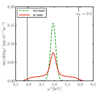
Figure 2: (Color online) Differential cross section (left panel in a log scale) as a function of $\omega^{\prime}$ for the fixed observation direction $\vartheta=90\mathrm{\SIUnitSymbolDegree}$ and $\varphi=45\mathrm{\SIUnitSymbolDegree}$ for $a_{L}=0.3$. The vertical dotted lines depict the cut-off values (25,26). The right panel shows, in a linear scale, the spectrum with $100\text{\,}\mathrm{eV}$ (rms Gaussian shape) resolution (red solid curve; for a comparison, the plain KN line without the laser is depicted as green dashed curve.

The unpolarized differential cross section is exhibited in Fig. 2 as a function of the frequency $\omega^{\prime}$ for a fixed observation direction $\vartheta=90\mathrm{\SIUnitSymbolDegree}$ and $\varphi=45\mathrm{\SIUnitSymbolDegree}$. The scattering angle $\vartheta$ is measured with respect to the beam axis $\mathbf{k}_{L}$; the azimuthal angle $\varphi$ w.r.t. $\mathbf{\epsilon}_{L}$. In the left panel of Fig. 2, for $a_{L}=0.3$ many side-lines form a roughened plateau, where the main KN line sticks out being very narrow as compared to the width of the plateau. The plateau spans the range $4\ldots 6\text{\,}\mathrm{keV}$, corresponding to the order of $$1\text{\,}\mathrm{keV}$/\omega_{L}\sim 650$ exchanged laser photons, despite of $a_{L}<1$. The right panel depicts the spectrum, averaged with a detector resolution of $100\text{\,}\mathrm{eV}$, on a linear scale. While the KN line becomes broader, the plateau is clearly visible and the roughness is averaged out (red curve). Compared to Compton scattering without the laser (green dashed curve), the peak height of the Klein Nishina line is reduced to half of its value (see also the discussion in Section IV.4)

To find the relevant multi-photon parameter for the process in Fig. 1(c) we determine the cut-off values $\ell_{\pm}$, beyond which the amplitude drops exponentially fast, via the stationary phase method by requiring that there are no stationary points $\phi_{\star}$ on the real axis, i.e. $\psi(\phi_{\star})=0$ (see Eq. (20)) has no real solutions. Abbreviating $f=g_{L}(\phi)\cos\phi$ we find

$$f(\phi_{\star})=-\frac{\alpha_{L}}{2\beta_{L}}\pm\sqrt{\frac{\alpha_{L}^{2}}{4\beta_{L}^{2}}-\frac{\ell}{\beta_{L}}}\,,$$ (24)

which has no real solutions for $\phi_{\star}$ if $(i)$ the term under the root becomes negative or $(ii)$ there are no real solutions when calculating the inverse function $f^{-1}$. The cut-off values are determined at maximum intensity at the center of the pulse, thus, we may set $g_{L}\to 1$ here and condition $(ii)$ turns into $|f|\leq 1$. We find

$$\ell_{-} =\frac{\varkappa\xi_{-}}{1-\xi_{-}}\,,$$ (25)

$$\ell_{+} =\left\{\begin{matrix}\displaystyle\frac{\varkappa\xi_{+}}{1-\xi_{+}}\,,&\quad\text{for }\vartheta\leq\vartheta_{\star}\,,\\ \displaystyle\frac{\varkappa\xi_{0}}{1-\xi_{0}}\,,&\quad\text{for }\vartheta>\vartheta_{\star}\end{matrix}\right.$$ (26)

with

$$\xi_{0} =\frac{\sin^{2}\vartheta\cos^{2}\varphi}{2-2\cos\vartheta}\,,$$ (27)

$$\xi_{\pm} =\frac{a_{L}^{2}}{2}(\cos\vartheta-1)\pm a_{L}\sin\vartheta|\cos\varphi|$$ (28)

and

$$\cos\vartheta_{\star} =\frac{a_{L}^{2}-\cos^{2}\varphi}{a_{L}^{2}+\cos^{2}\varphi}\,.$$ (29)

For $a_{L}<1$, the cut-off values are of the order $\varkappa a_{L}$ for most observation angles. Thus, for moderately strong laser fields and a large frequency ratio the relevant multi-photon parameter is $\varkappa a_{L}$. This is in severe contrast to the spontaneous process $S_{0}$ depicted in Fig. 1(b), where the multi-photon parameter is $a_{L}$ Ritus (1985).

IV.3 Angular spectra

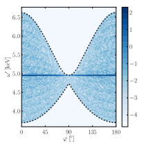
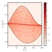
Figure 3: (Color online) Frequency vs. angle correlations of the cross section as a function of the azimuthal angle for fixed $\vartheta=90\mathrm{\SIUnitSymbolDegree}$ (left panel) and as a function of $\vartheta$ for fixed $\varphi=45\mathrm{\SIUnitSymbolDegree}$ (right panel) for $a_{L}=0.3$. The cutoff-values (25,26) are depicted by the dotted curves. The color scale represents $\log_{10}({\mathrm{d}}\sigma/{\mathrm{d}}\Omega{\mathrm{d}}\omega^{\prime}\usk[\mathrm{m}\mathrm{b}\usk\mathrm{eV}^{-1}\mathrm{sr}^{-1}])$.

The plateau has a pronounced dependence on the azimuthal angle $\varphi$, see left panel of Fig. 3. A strong reduction of the plateau width is observed at $\varphi=90\mathrm{\SIUnitSymbolDegree}$, i.e. perpendicularly to the laser polarization, where $\ell_{+}=0$. The broadest plateau is found close to the laser polarization direction which is perpendicular to the X-ray polarization where up to $1000$ laser photons participate. The polar angle distribution (right panel) shows a forward-backward asymmetry. For large scattering angles $\vartheta>90\mathrm{\SIUnitSymbolDegree}$ the emission with $\ell>0$, i.e. $\omega^{\prime}>\omega^{\prime}_{\rm KN}$ is suppressed. The cut-off values (25,26), depicted by dotted curves, coincide with the numerical results. From our analysis of the angular spectra we propose to choose as observation direction $\vartheta=90\mathrm{\SIUnitSymbolDegree}$ and an azimuthal angle not too close to $\varphi=90\mathrm{\SIUnitSymbolDegree}$, e.g. as discussed above in Fig. 2, to optimize the width of the plateau.

IV.4 Energy Integrated Cross Section

Numerically we find that the energy integrated cross section equals the KN cross section Berestetzki et al. (1980), i.e.

$$\int\!{\mathrm{d}}\omega^{\prime}\,\frac{{\mathrm{d}}\sigma}{{\mathrm{d}}\Omega{\mathrm{d}}\omega^{\prime}}=\frac{d\sigma_{\rm KN}}{{\mathrm{d}}\Omega}\,.$$ (30)

A qualitative argument for this behavior is provided by a classical model, where the total emitted power $\dot{E}$ is given by the Larmor formula yielding

$$\dot{E} =-\frac{e^{4}}{6\pi m^{2}}(A^{\prime}_{L}\cdot A^{\prime}_{L}+A^{\prime}_{X}\cdot A^{\prime}_{X})\,,$$ (31)

where primes denote derivatives w.r.t. $\phi$. The first term in brackets corresponds to the spontaneous emission process and the second term refers to the laser assisted Compton scattering of X-ray photons $S_{+1}$. The latter part is independent of the laser intensity. Such a redistribution in phase space with marginal impact on the total probability has been found also for other laser assisted processes Lötstedt et al. (2008).

To quantify the fraction of photons scattered into the side-bands, in particular for the observation direction used in Fig. 2, we define the side-band cross section as that part of the spectrum which is at least by $\pm\omega_{L}/2$ away from $\omega^{\prime}_{\rm KN}$. (A variation of the discrimination value in the range $0.25\ldots 0.75\,\omega_{L}$ leads to a relative uncertainty of $\leq 5\%$.) For small values of $\varkappa a_{L}\ll 1$, the side-band fraction scales as $a_{L}^{2}$. For larger values of $a_{L}$, the main line is weakened, see right panel in Fig. 2. (For monochromatic waves, where $g_{X,L}\to 1$, also a negative lowest-order $a_{L}$ corrections to the main line has been found Guccione-Gush and Gush (1975); Akhiezer and Merenkov (1985)). The side-band cross section increases with $a_{L}$ up to $a_{L}\sim 0.01$, where it saturates at $30\text{\,}\mathrm{m}\mathrm{b}\usk\mathrm{sr}^{-1}$. This value should be compared to the corresponding KN cross section (without the laser) of $39\text{\,}\mathrm{m}\mathrm{b}\usk\mathrm{sr}^{-1}$, proving that a large fraction of the photons is emitted into the side-bands.

IV.5 Polarization

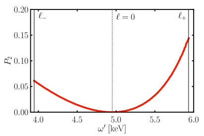
Figure 4: (Color online) Rotation of the polarization of the scattered photon, quantified via the Stokes parameter $P_{2}$ as a function of $\omega^{\prime}$ for the same observation direction as in Fig. 2.

Due to the non-linear mixing of optical laser photons with the incident X-ray photon the polarization of the photon $X^{\prime}$ is rotated as compared to Compton scattering without the laser. The rotation angle is frequency dependent. This rotation can be quantified experimentally by measuring the Stokes parameter $P_{2}$ which we calculate as $P_{2}=(w_{45\mathrm{\SIUnitSymbolDegree}}-w_{135\mathrm{\SIUnitSymbolDegree}})/(w_{45\mathrm{\SIUnitSymbolDegree}}+w_{135\mathrm{\SIUnitSymbolDegree}})$, where $w_{\chi}$ denotes the triple differential cross section of photons with their polarization vector having an angle of $\chi$ w.r.t. the scattering plane. For instance, for the observation angles of Fig. 2 the photon $X^{\prime}$ is polarized perpendicular to the scattering plane without the laser which means $P_{2}=0$. This result is changed in laser assisted Compton scattering. In Fig. 4 the Stokes parameter $P_{2}$ is exhibited as a function of $\omega^{\prime}$ for $a_{L}=0.3$. The value of $P_{2}$ is zero at the KN line and increases with increasing distance from it, i.e., in the region where more laser photons are involved. The maximum value of $P_{2}$ corresponds to a rotation angle of $5\mathrm{\SIUnitSymbolDegree}$ towards $\mathbf{k}_{L}$. In the classical picture, the figure-8 orbit in the laser field has a component in the directions of $\mathbf{k}_{L}$ which is transferred to the polarization of the photon $X^{\prime}$. The energy dependent polarization rotation can be used to identify unambiguously the final state photons emerging from the multi-photon process.

V Discussion and Summary

A clear and easily observable signature of laser assisted Compton scattering of X-ray photons is provided by the side-lines accompanying the main Klein-Nishina line forming a broad plateau. Due to the difference of scales of the photon energies of X-ray and optical laser, non-linear effects are strongly enhanced as compared to the spontaneous emission of radiation in a pure laser field. The relevant multi-photon parameter is $\varkappa a_{L}$, which can be large even for laser fields with intensities of the order of $10^{18}\text{\,}\mathrm{W}\mathrm{/}\mathrm{c}\mathrm{m}^{2}$. The optimal conditions to observe the side-band plateau with an X-ray camera are achieved for $a_{L}\lesssim 1$. Such intensities are achieved routinely with a $200\text{\,}\mathrm{TW}$ laser in relatively large spot sizes of $w_{0}=\mathcal{O}($100\text{\,}\mathrm{\SIUnitSymbolMicro m}$)$ and pulse lengths of $T_{L}=$20\text{\,}\mathrm{fs}$$. We do not expect that spatially inhomogeneous laser spots influence the cut-off values since they are sensitive to the maximum laser intensity in the spatio-temporal profile of the pulse. However, the shape of the plateau will certainly change. The optical photons emerging from spontaneous emission process, i.e. the non-linear Compton process exhibited in Fig. 1(b), can be efficiently filtered out by a thin foil which is otherwise transparent for X-rays.

A very useful signal for the non-linear frequency mixing is the frequency dependent rotation of the polarization of the final state photons. The polarization can be measured by using X-ray polarizers. A polarization purity of the order of $10^{-10}$ has been achieved recently Marx et al. (2013). The technique of a polarization veto can be used to shield the plain KN photons (arising for unsynchronized X and L pulses) or shield the $\ell=0$ KN-like photons. For optimal conditions, the X-ray pulse length $T_{X}$ and the laser pulse length $T_{L}$ should be of the same order of magnitude. The synchronization of optical and X-ray pulses to the level of femtoseconds has been achieved experimentally Tavella et al. (2011), approaching the sub-femtosecond level Schultze et al. (2010). Numerically, the spectra are insensitive to a temporal offset between the two pulses of the order of a few femtoseconds.

A slight misalignment of the X-ray and laser beams due to axis off-sets or focusing effects does not lead to qualitatively new effects: The Oleinik resonances Oleĭnik (1968) for non-parallel beams (see e.g. Hartin (2006); Voroshilo and Roshchupkin (2005); Voroshilo et al. (2011); Nedoreshta et al. (2013b)) are suppressed by the large frequency ratio $\varkappa$ and for a small angular misalignment $\Theta\ll 1$ between the X-ray and laser beams. A slight misalignment of the polarizations, $\mathbf{\epsilon}_{X}\cdot\mathbf{\epsilon}_{L}\neq 0$, causes laser intensity dependent modifications of the total cross section of the order ${\cal O}(\mathbf{\epsilon}_{X}\cdot\mathbf{\epsilon}_{L})\ll 1$.

Such experiments can be performed at LCLS or at the European XFEL combining the X-ray facility with an optical laser system, e.g., as planned in HIBEF sit . One could employ low-energy electrons emitted from an electron gun as in the experiment Englert and Rinehart (1983). However, the electron energy cannot be too low since low energy-electrons are expelled from high-intensity regions due to the ponderomotive force. We found numerically that for electron kinetic energies as low as $E_{\rm kin}=$500\text{\,}\mathrm{eV}$$ the electrons can penetrate the focus and the maximum deflection angle is below $0.8\text{\,}\mathrm{\SIUnitSymbolDegree}$. This is due to the fact that the transverse ponderomotive force which is responsible for the deflection is proportional to the gradient of the laser intensity and scales as $\propto a_{L}^{2}/w_{0}$, where $a_{L}$ is rather small and the laser spot size $w_{0}$ is large. Consequently, electrons with kinetic energies of a few hundred $\mathrm{eV}$ are suitable for such experiments.

In conclusion, studying the laser assisted Compton scattering of X-rays will significantly advance our understanding of strong-field QED scattering processes in the ${\cal O}(10^{3})$ multi-photon regime.

VI Acknowledgements

The authors are grateful to T. E. Cowan and R. Sauerbrey for the inspiring collaboration on future experiments at HIBEF. DS acknowledges stimulating discussions with S. Fritzsche, A. Surzhykov and V. G. Serbo.

Appendix A The limit of infinite monochromatic plane waves

In this appendix we discuss briefly the limit of infinite monochromatic plane waves (IPW), $T_{X},T_{L}\to\infty$. In this case, characterized by $g_{L,X}\to 1$, the integral in the exponents of the functions $C_{n}$, Eq. (19), is given by

$$\int\!{\mathrm{d}}\phi\,\psi_{\rm IPW}(\phi) =\ell\phi+\alpha_{L}\sin\phi+\frac{\beta_{L}}{2}\phi+\frac{\beta_{L}}{4}\sin 2\phi\,.$$ (32)

Owing to the periodicity of the monochromatic field, the integrand of the $C_{n}$ can be expanded in a discrete Fourier series, excluding the non-periodic terms in (32), such that the integrals $C_{n}$ turn into a sum over discrete partial amplitudes. For instance, for $C_{0}$ we find

$$C_{0}^{\rm IPW}=\sum_{N=-\infty}^{\infty}2\pi\delta(\ell-N+\beta_{L}/2)J_{N}(\alpha_{L},\beta_{L})$$ (33)

with amplitudes

$$J_{N}(\alpha_{L},\beta_{L})=\sum_{s=-\infty}^{\infty}J_{N-2s}(-\alpha_{L})J_{s}(-\beta_{L}/4)$$ (34)

and the Bessel functions $J_{N}$. Similar relations can be found for all integrals $C_{n}^{\rm IPW}$. Thus, in the limit of infinite plane waves the variable $\ell$ becomes a discrete $\ell_{N}=N-\beta_{L}/2$, with integer values of $N$, due to $\delta(\ell-N+\beta_{L}/2)$. The term $\beta_{L}/2$ can be absorbed into the electron momenta leading to the occurrence of the field-dressed quasi-momentum

$$\tilde{p}=p+\frac{m^{2}a_{L}^{2}}{4k_{L}\cdot p}k_{L}\,,$$ (35)

and similarly for $p^{\prime}$. The formal energy momentum conservation (5) turns into

$$\tilde{p}+k_{X}+Nk_{L}=\tilde{p}^{\prime}+k^{\prime}\,,$$ (36)

where $N$ can be considered as number of laser photons exchanged during the scattering process, as pointed out e.g. in Mackenroth and Di Piazza (2011); Harvey et al. (2012) for non-linear Compton scattering. Solving (36) for the frequency $\omega^{\prime}$ gives

$$\omega^{\prime}_{N}(\vartheta)=\frac{\omega_{X}+N\omega_{L}}{1+\left(\frac{\omega_{X}+N\omega_{L}}{m}+\frac{a_{L}^{2}}{4}\right)(1-\cos\vartheta)}\,,$$ (37)

i.e. discrete frequencies $\omega^{\prime}_{N}$ with an intensity dependent red-shift quantified by the term $a_{L}^{2}/4$ in the denominator Ehlotzky (1989).

Integrating over ${\mathrm{d}}\ell$ in (17) and exploiting the delta distributions in the functions $C_{n}^{\rm IPW}$, the amplitude $M$, Eq. (18), becomes a sum of discrete partial amplitudes

$$M_{\rm IPW}=\sum_{N}M_{N}\,.$$ (38)

The same is true for the cross section

$$\frac{{\mathrm{d}}\sigma_{\rm IPW}}{{\mathrm{d}}\Omega}=\sum_{N}\frac{{\mathrm{d}}\sigma_{N}}{{\mathrm{d}}\Omega}\,,$$ (39)

as known from the literature, e.g. Guccione-Gush and Gush (1975); Akhiezer and Merenkov (1985); Ehlotzky (1989). The dependence on $\omega^{\prime}$ in (23) is replaced by a sum over discrete values of $N$. This shows that our results for pulsed plane waves, in particular (17), (18) and (23), contain also the known case of infinite plane waves in the proper limit.

References

- Compton (1923) A. H. Compton, Phys. Rev. 21, 483 (1923).
- Ehlotzky (1987) F. Ehlotzky, J. Phys. B 20, 2619 (1987).
- Weingartshofer et al. (1977) A. Weingartshofer, J. K. Holmes, G. Caudle, E. M. Clarke, and H. Krüger, Phys. Rev. Lett. 39, 269 (1977).
- Taïeb et al. (2008) R. Taïeb, A. Maquet, and M. Meyer, J. Phys. Conf. Ser. 141, 012017 (2008).
- Sarachik and Schappert (1970) E. S. Sarachik and G. T. Schappert, Phys. Rev. D 1, 2738 (1970).
- Di Piazza et al. (2012) A. Di Piazza, C. Müller, K. Z. Hatsagortsyan, and C. H. Keitel, Rev. Mod. Phys. 84, 1177 (2012).
- Oleĭnik (1968) V. P. Oleĭnik, Sov. Phys. JETP 26, 1132 (1968).
- Guccione-Gush and Gush (1975) R. Guccione-Gush and H. P. Gush, Phys. Rev. D 12, 404 (1975).
- Akhiezer and Merenkov (1985) A. I. Akhiezer and N. P. Merenkov, Sov. Phys. JETP 61, 41 (1985).
- Puntajer and Leubner (1989) A. K. Puntajer and C. Leubner, Phys. Rev. A 40, 279 (1989).
- Ehlotzky (1989) F. Ehlotzky, J. Phys. B 22, 601 (1989).
- Zhukovskii and Nikitina (1973) V. C. Zhukovskii and N. S. Nikitina, Sov. Phys. JETP 37, 595 (1973).
- Baier et al. (1998) V. N. Baier, V. M. Katkov, and V. M. Strakhovenko, Electromagnetic Processes at High Energies in Oriented Single Crystals (World Scientific Publishing, 1998).
- Nedoreshta et al. (2013a) V. N. Nedoreshta, S. P. Roshchupkin, and A. I. Voroshilo, Laser Phys. 23, 055301 (2013a).
- Narozhnyi and Fofanov (1996) N. B. Narozhnyi and M. S. Fofanov, JETP 83, 14 (1996).
- Boca and Florescu (2009) M. Boca and V. Florescu, Phys. Rev. A 80, 053403 (2009).
- Heinzl et al. (2010a) T. Heinzl, D. Seipt, and B. Kämpfer, Phys. Rev. A 81, 022125 (2010a).
- Seipt and Kämpfer (2011) D. Seipt and B. Kämpfer, Phys. Rev. A 83, 022101 (2011).
- Mackenroth and Di Piazza (2011) F. Mackenroth and A. Di Piazza, Phys. Rev. A 83, 032106 (2011).
- Krajewska and Kamiński (2012a) K. Krajewska and J. Z. Kamiński, Phys. Rev. A 85, 062102 (2012a).
- Seipt and Kämpfer (2013) D. Seipt and B. Kämpfer, Phys. Rev. A 88, 012127 (2013).
- Heinzl et al. (2010b) T. Heinzl, A. Ilderton, and M. Marklund, Phys. Lett. B 692, 250 (2010b).
- Nousch et al. (2012) T. Nousch, D. Seipt, B. Kämpfer, and A. I. Titov, Phys. Lett. B 715, 246 (2012).
- Krajewska et al. (2013) K. Krajewska, C. Müller, and J. Z. Kamiński, Phys. Rev. A 87, 062107 (2013).
- Kohlfürst et al. (2013) C. Kohlfürst, M. Mitter, G. von Winckel, F. Hebenstreit, and R. Alkofer, Phys. Rev. D 88, 045028 (2013).
- Ilderton et al. (2011) A. Ilderton, P. Johansson, and M. Marklund, Phys. Rev. A 84, 032119 (2011).
- Volkov (1935) D. M. Volkov, Z. Phys. 94, 250 (1935).
- Voroshilo and Roshchupkin (1996) A. I. Voroshilo and S. P. Roshchupkin, Laser Phys. 7, 466 (1996).
- Krajewska and Kamiński (2012b) K. Krajewska and J. Z. Kamiński, Phys. Rev. A 85, 043404 (2012b).
- Augustin and Müller (2013) S. Augustin and C. Müller, Phys. Rev. A 88, 022109 (2013).
- Voroshilo et al. (2013) A. I. Voroshilo, S. P. Roshchupkin, and V. N. Nedoreshta, in Proceedings of the 12th International Conference on Laser and Fiber-Optical Networks Modeling (2013) p. 32.
- Herrmann and Zhukovskii (1972) J. Herrmann and V. C. Zhukovskii, Ann. Phys. (Leipzig) 482, 349 (1972).
- Hu and Müller (2011) H. Hu and C. Müller, Phys. Rev. Lett. 107, 090402 (2011).
- Note (1) There are corrections to that process of the order of when arranging the expansion of Fig. 1(a) according to the energy-momentum balance Herrmann and Zhukovskii (1972).
- Brown and Kibble (1964) L. S. Brown and T. W. B. Kibble, Phys. Rev. 133, A705 (1964).
- Narozhnyi et al. (1965) N. B. Narozhnyi, A. I. Nikishov, and V. I. Ritus, Sov. Phys. JETP 20, 622 (1965).
- Harvey et al. (2009) C. Harvey, T. Heinzl, and A. Ilderton, Phys. Rev. A 79, 063407 (2009).
- Englert and Rinehart (1983) T. J. Englert and E. A. Rinehart, Phys. Rev. A 28, 1539 (1983).
- Bula et al. (1996) C. Bula et al., Phys. Rev. Lett. 76, 3116 (1996).
- Chen et al. (1998) S.-Y. Chen, A. Maksimchuk, and D. Umstadter, Nature 396, 653 (1998).
- Harvey et al. (2012) C. Harvey, T. Heinzl, A. Ilderton, and M. Marklund, Phys. Rev. Lett. 109, 100402 (2012).
- Ilderton (2011) A. Ilderton, Phys. Rev. Lett. 106, 020404 (2011).
- Lötstedt and Jentschura (2009) E. Lötstedt and U. D. Jentschura, Phys. Rev. Lett. 103, 110404 (2009).
- Seipt and Kämpfer (2012) D. Seipt and B. Kämpfer, Phys. Rev. D 85, 101701 (2012).
- Mackenroth and Di Piazza (2013) F. Mackenroth and A. Di Piazza, Phys. Rev. Lett. 110, 070402 (2013).
- Klein and Nishina (1929) O. Klein and Y. Nishina, Z. Phys. 52, 853 (1929).
- (47) “The HIBEF project,” www.hzdr.de/hgfbeamline/.
- (48) “The European XFEL project,” http://www.xfel.eu/.
- Ritus (1985) V. I. Ritus, J. Sov. Laser Res. 6, 497 (1985).
- Berestetzki et al. (1980) W. B. Berestetzki, E. M. Lifschitz, and L. P. Pitajewski, Relativistische Qantentheorie, Lehrbuch der Theoretischen Physik, Vol. IV (Akademie Verlag, Berlin, 1980).
- Lötstedt et al. (2008) E. Lötstedt, U. D. Jentschura, and C. H. Keitel, Phys. Rev. Lett. 101, 203001 (2008).
- Marx et al. (2013) B. Marx et al., Phys. Rev. Lett. 110, 254801 (2013).
- Tavella et al. (2011) F. Tavella, N. Stojanovic, G. Geloni, and M. Gensch, Nature Photon. 5, 162 (2011).
- Schultze et al. (2010) M. Schultze et al., Science 328, 1658 (2010).
- Hartin (2006) A. Hartin, Second Order QED Processes in an Intense Electromagnetic Field, Ph.D. thesis, University of London (2006).
- Voroshilo and Roshchupkin (2005) A. I. Voroshilo and S. P. Roshchupkin, Laser Phys. Lett. 2, 184 (2005).
- Voroshilo et al. (2011) A. I. Voroshilo, S. P. Roshchupkin, and V. N. Nedoreshta, Laser Phys. 21, 1675 (2011).
- Nedoreshta et al. (2013b) V. N. Nedoreshta, A. I. Voroshilo, and S. P. Roshchupkin, Phys. Rev. A 88, 052109 (2013b).