Structure Learning of Probabilistic Logic Programs by Searching the Clause Space

Abstract

Learning probabilistic logic programming languages is receiving an increasing attention and systems are available for learning the parameters (PRISM, LeProbLog, LFI-ProbLog and EMBLEM) or both the structure and the parameters (SEM-CP-logic and SLIPCASE) of these languages. In this paper we present the algorithm SLIPCOVER for “Structure LearnIng of Probabilistic logic programs by searChing OVER the clause space”. It performs a beam search in the space of probabilistic clauses and a greedy search in the space of theories, using the log likelihood of the data as the guiding heuristics. To estimate the log likelihood SLIPCOVER performs Expectation Maximization with EMBLEM. The algorithm has been tested on five real world datasets and compared with SLIPCASE, SEM-CP-logic, Aleph and two algorithms for learning Markov Logic Networks (Learning using Structural Motifs (LSM) and ALEPH++ExactL1). SLIPCOVER achieves higher areas under the precision-recall and ROC curves in most cases.

Note: This article will appear in Theory and Practice of Logic Programming, ©Cambridge University Press.

1 Introduction

Recently much work in Machine Learning has concentrated on representation languages able to combine aspects of logic and probability, leading to the birth of a whole field called Statistical Relational Learning (SRL). The ability to model both complex and uncertain relationships among entities is very important for learning accurate models of many domains. The standard frameworks for handling these features are first-order logic and probability theory respectively. Thus we would like to be able to learn and perform inference in languages that integrate the two, unlike traditional Inductive Logic Programming (ILP) methods which only address the complexity issue.

Probabilistic Logic Programming (PLP) has recently received an increasing attention for its ability to incorporate probability in logic programming. Among various proposals for PLP, the one based on the distribution semantics [Sato (1995)] is gaining popularity and is the basis for languages such as Probabilistic Logic Programs [Dantsin (1991)], Probabilistic Horn Abduction [Poole (1993)], PRISM [Sato (1995)], Independent Choice Logic [Poole (1997)], pD [Fuhr (2000)], Logic Programs with Annotated Disjunctions (LPADs) [Vennekens et al. (2004)], ProbLog [De Raedt et al. (2007)] and CP-logic [Vennekens et al. (2009)].

Inference for PLP languages can be performed with a number of algorithms, which in many cases find explanations for queries and compute their probability by building a Binary Decision Diagram (BDD) [De Raedt et al. (2007), Riguzzi (2007), Kimmig et al. (2011), Riguzzi and Swift (2011)].

Various works have started to appear on the problem of learning the parameters of PLP languages under the distribution semantics: LeProbLog [Gutmann et al. (2008)] uses gradient descent while LFI-ProbLog [Gutmann et al. (2011)] and EMBLEM [Bellodi and Riguzzi (2012), Bellodi and Riguzzi (2013)] use an Expectation Maximization approach where the expectations are computed directly from BDDs.

The problem of learning the structure of these languages is also becoming of interest, with works such as [De Raedt et al. (2008)], where a theory compression algorithm for ProbLog is presented, and [Meert et al. (2008)], where ground LPADs are learned using Bayesian Networks techniques. SLIPCASE [Bellodi and Riguzzi (2011)] also learns the structure of LPADs by performing a beam search in the space of probabilistic theories using the log likelihood (LL) of the data as the guiding heuristics. To estimate the LL, it performs a limited number of Expectation Maximization iterations of EMBLEM.

The structure learning task may be addressed with a discriminative or generative approach. A discriminative learning problem is characterized by specific target predicate(s) that must be predicted. The search for clauses is directly guided by the goal of maximizing the predictive accuracy of the resulting theory on the target predicates. A generative learner attempts, on the contrary, to learn a theory that is equally capable of predicting the truth value of all predicates.

In this paper we propose an evolution of SLIPCASE called SLIPCOVER, for “Structure LearnIng of Probabilistic logic programs by searChing OVER the clause space”. SLIPCASE is based on a simple search strategy that iteratively performs theory revision. Differently from it, SLIPCOVER first searches the space of clauses storing all the promising ones, dividing them into clauses for target predicates (those we want to predict) and clauses for background predicates (the remaining ones), with a discriminative approach. This search starts from a set of “bottom clauses” generated as in Progol [Muggleton (1995)] and looks for good refinements in terms of LL. Then it performs a greedy search in the space of theories, by trying to add each clause for a target predicate to the current theory. Finally, it performs parameter learning with EMBLEM on the best target theory plus the clauses for background predicates. SLIPCOVER can learn general LPADs including non-ground programs.

Finally, Markov Logic Networks (MLNs) are a recently developed SRL model that generalizes both first order logic and Markov networks [Richardson and Domingos (2006)], for which several parameter and structure learning algorithms have been proposed.

The aim of the paper is to demonstrate that a system based on ILP and PLP is competitive or superior to existing purely ILP or SRL methods. Moreover, the paper shows how the improved search strategy implemented in SLIPCOVER produces superior results with respect to the simpler SLIPCASE.

The paper is organized as follows. Section 2 presents Probabilistic Logic Programming, concentrating on LPADs. Section 3 describes EMBLEM in details. Section 4 illustrates SLIPCOVER while Section 5 discusses related work. In Section 6 we present the results of the experiments. Section 7 concludes the paper and proposes directions for future work.

2 Probabilistic Logic Programming

The distribution semantics [Sato (1995)] is one of the most interesting approaches to the integration of logic programming and probability. It was introduced for the PRISM language but is shared by many other languages. A program in one of these languages defines a probability distribution over normal logic programs called instances. Each normal program is assumed to have a total well-founded model [Van Gelder et al. (1991)] thus each program can be associated with a Herbrand interpretation (a world) that is its model and the distribution over instances directly translates into a distribution over Herbrand interpretations. Then, the distribution is extended to queries and the probability of a query is obtained by marginalizing the joint distribution of the query and the programs. The languages following the distribution semantics differ in the way they define the distribution over logic programs but have the same expressive power: there are transformations with linear complexity that can convert each one into the others [Vennekens and Verbaeten (2003), De Raedt et al. (2008)]. In this paper we will use LPADs for their general syntax. We review here the semantics in the case of no function symbols for the sake of simplicity.

In LPADs the alternatives are encoded in the head of clauses in the form of a disjunction in which each atom is annotated with a probability. Formally a Logic Program with Annotated Disjunctions $T$ consists of a finite set of annotated disjunctive clauses [Vennekens et al. (2004)]. An annotated disjunctive clause $C_{i}$ is of the form

$$h_{i1}:\Pi_{i1};\ldots;h_{in_{i}}:\Pi_{in_{i}}\ {:\!-}\ b_{i1},\ldots,b_{im_{i}}$$

In such a clause, $h_{i1},\ldots,h_{in_{i}}$ are logical atoms, $b_{i1},\ldots,b_{im_{i}}$ are logical literals and $\{\Pi_{i1},\ldots,\Pi_{in_{i}}\}$ are real numbers in the interval $[0,1]$ such that $\sum_{k=1}^{n_{i}}\Pi_{ik}\leq 1$; $b_{i1},\ldots,b_{im_{i}}$ is indicated with $body(C_{i})$. Note that, if $n_{i}=1$ and $\Pi_{i1}=1$, the clause corresponds to a non-disjunctive clause. If $\sum_{k=1}^{n_{i}}\Pi_{ik}<1$, the head of the annotated disjunctive clause implicitly contains an extra atom $null$ that does not appear in the body of any clause and whose annotation is $1-\sum_{k=1}^{n_{i}}\Pi_{ik}$. We denote by $ground(T)$ the grounding of an LPAD $T$.

An atomic choice [Poole (1997)] is a triple $(C_{i},\theta_{j},k)$ where $C_{i}\in T$, $\theta_{j}$ is a substitution that grounds $C_{i}$ and $k\in\{1,\ldots,n_{i}\}$ identifies one of the head atoms. In practice $C_{i}\theta_{j}$ corresponds to a random variable $X_{ij}$ and an atomic choice $(C_{i},\theta_{j},k)$ to an assignment $X_{ij}=k$. A set of atomic choices $\kappa$ is consistent if only one head is selected from the same ground clause; we assume independence between the different choices. A composite choice $\kappa$ is a consistent set of atomic choices [Poole (1997)]. The probability $P(\kappa)$ of a composite choice $\kappa$ is the product of the probabilities of the independent atomic choices, i.e. $P(\kappa)=\prod_{(C_{i},\theta_{j},k)\in\kappa}\Pi_{ik}$.

A selection $\sigma$ is a composite choice that, for each clause $C_{i}\theta_{j}$ in $ground(T)$, contains an atomic choice $(C_{i},\theta_{j},k)$. Let us indicate with $S_{T}$ the set of all selections. A selection $\sigma$ identifies a normal logic program $l_{\sigma}$ defined as $l_{\sigma}=\{(h_{ik}\leftarrow body(C_{i}))\theta_{j}|(C_{i},\theta_{j},k)\in\sigma\}$. $l_{\sigma}$ is called an instance of $T$. Since selections are composite choices, we can assign a probability to instances: $P(l_{\sigma})=P(\sigma)=\prod_{(C_{i},\theta_{j},k)\in\sigma}\Pi_{ik}$.

We consider only sound LPADs as defined below.

Definition 1

An LPAD $T$ is called $sound$ iff for each selection $\sigma$ in $S_{T}$, the well-founded model of the program $l_{\sigma}$ chosen by $\sigma$ is two-valued.

A particularly loose sufficient condition for the soundness of LPADs is the bounded term-size property, defined in [Riguzzi and Swift (2013)], which is based on a characterization of the well-founded semantics in terms of an iterated fixpoint [Przymusinski (1989)]. A bounded term-size program is such that in each iteration of the fixpoint the size of true atoms does not grow indefinitely. LPAD without negation in clauses’ bodies are sound, as the well-founded model coincides with the least Herbrand model.

We write $l_{\sigma}\models Q$ to mean that the query $Q$ is true in the well-founded model of the program $l_{\sigma}$.

We denote the set of all instances by $L_{T}$. A composite choice $\kappa$ identifies a set of instances $\lambda_{\kappa}=\{l_{\sigma}|\sigma\in S_{T},\sigma\supseteq\kappa\}$. We define the set of instances identified by a set of composite choices $K$ as $\lambda_{K}=\bigcup_{\kappa\in K}\lambda_{\kappa}$.

Let $P(L_{T})$ be the distribution over instances. The probability of a query $Q$ given an instance $l$ is $P(Q|l)=1$ if $l\models Q$ and 0 otherwise. The probability of a query $Q$ is given by

$$P(Q)=\sum_{l\in L_{T}}P(Q,l)=\sum_{l\in L_{T}}P(Q|l)P(l)=\sum_{l\in L_{T}:l\models Q}P(l)$$ (1)

Example 1

The following LPAD $T$ is inspired by the morphological characteristics of the Stromboli Italian island:

$\begin{array}[]{llll}C_{1}&=&eruption:0.6\ ;\ earthquake:0.3\ {:\!-}\ sudden\_energy\_release,\\ &&fault\_rupture(X).\\ C_{2}&=&sudden\_energy\_release:0.7.\\ C_{3}&=&fault\_rupture(southwest\_northeast).\\ C_{4}&=&fault\_rupture(east\_west).\end{array}$

The Stromboli island is located at the intersection of two geological faults, one in the southwest-northeast direction, the other in the east-west direction, and contains one of the three volcanoes that are active in Italy. This program models the possibility that an eruption or an earthquake occurs at Stromboli. If there is a sudden energy release under the island and there is a fault rupture ($C_{1}$), then there can be an eruption of the volcano on the island with probability 0.6 or an earthquake in the area with probability 0.3 or no event (the implicit $null$ atom) with probability 0.1. The energy release occurs with probability 0.7 while we are sure that ruptures occur in both faults.

Clause $C_{1}$ has two groundings, $C_{1}\theta_{1}$ with $\theta_{1}=\{X/southwest\_northeast\}$ and $C_{1}\theta_{2}$ with $\theta_{2}=\{X/east\_west\}$, so there are two random variables $X_{11}$ and $X_{12}$. Clause $C_{2}$ has only one grounding $C_{2}\emptyset$ instead, so there is one random variable $X_{21}$. $X_{11}$ and $X_{12}$ can take on three values since $C_{1}$ has three head atoms; similarly $X_{21}$ can take on two values since $C_{2}$ has two head atoms. $T$ has 18 instances, the query $eruption$ is true in 5 of them and its probability is

$P(eruption)=0.6\cdot 0.6\cdot 0.7+0.6\cdot 0.3\cdot 0.7+0.6\cdot 0.1\cdot 0.7+0.3\cdot 0.6\cdot 0.7+0.1\cdot 0.6\cdot 0.7=0.588.$ For instance, the second term of $P(eruption)$ corresponds to the following instance of $T$:

$\begin{array}[]{llll}C_{11}&=&eruption{:\!-}\ sudden\_energy\_release,\\ &&fault\_rupture(southwest\_northeast).\\ C_{12}&=&earthquake{:\!-}sudden\_energy\_release,fault\_rupture(east\_west).\\ C_{2}&=&sudden\_energy\_release.\\ C_{3}&=&fault\_rupture(southwest\_northeast).\\ C_{4}&=&fault\_rupture(east\_west).\end{array}$

As this example shows, multiple-head atoms are particularly useful when clauses have a causal interpretation: the body represents an event that, when happening, has a random consequence among those in the head. In addition, note that this LPAD allows the events eruption and earthquake to occurr at the same time, by virtue of the multiple groundings of clause $C_{1}$, as the above instance shows.

The semantics associates one random variable with every grounding of a clause. In some domains, this may result in too many random variables. In order to contain the number of variables and thus simplify inference, we may introduce an approximation at the level of the instantiations, by grounding only some of the variables of the clauses, at the expenses of the accuracy in modeling the domain. A typical compromise between accuracy and complexity is to consider the grounding of variables in the head only: in this way, a ground atom entailed by two separate ground instances of a clause is assigned the same probability, all other things being equal, of a ground atom entailed by a single ground clause, while in the “standard” semantics the first would have a larger probability, as more evidence is available for its entailment. This “approximate” semantics can be interpreted as stating that a ground atom is entailed by a clause with the probability given by its annotation if there is at least one substitution for the variables appearing only in the body such that the body is true. We have adopted this semantics in some experiments with SLIPCOVER and SLIPCASE in Section 6.

Example 2 (Example 1 cont.)

In the approximate semantics, $C_{1}$ is associated with a single random variable $X_{11}$. In this case $T$ has 6 instances, the query $eruption$ is true in 1 of them and its probability is $P(eruption)=0.6\cdot 0.7=0.42.$ So $eruption$ is assigned a lower probability with respect to the standard semantics because the two independent groundings of clause $C_{1}$, differing in the fault name, are not considered separately.

In practice inference algorithms find explanations for a query: a composite choice $\kappa$ is an explanation for a query $Q$ if $Q$ is entailed by every instance of $\lambda_{\kappa}$. In particular, algorithms find a covering set of explanations for the query, where a set of composite choices $K$ is covering with respect to $Q$ if every program $l_{\sigma}$ in which $Q$ is entailed is in $\lambda_{K}$. The problem of computing the probability of a query $Q$ can thus be reduced to computing the probability of the Boolean function

$$f_{Q}(\mathbf{X})=\bigvee_{\kappa\in E(Q)}\bigwedge_{(C_{i},\theta_{j},k)\in\kappa}X_{ij}=k$$ (2)

where $E(Q)$ is a covering set of explanations for $Q$.

Example 3 (Example 1 cont.)

The query $eruption$ has the covering set of explanations $E(eruption)=\{\kappa_{1},\kappa_{2}\}$ where:

$$\begin{array}[]{llll}\kappa_{1}&=&\{(C_{1},\{X/southwest\_northeast\},1),(C_{2},\{\},1)\}\\ \kappa_{2}&=&\{(C_{1},\{X/east\_west\},1),(C_{2},\{\},1)\}\end{array}$$

Each atomic choice $(C_{i},\theta_{j},k)$ is represented by the propositional equation $X_{ij}=k$:

$$\begin{array}[]{llll}(C_{1},\{X/southwest\_northeast\},1)&\rightarrow&X_{11}=1\\ (C_{1},\{X/east\_west\},1)&\rightarrow&X_{12}=1\\ (C_{2},\{\},1)&\rightarrow&X_{21}=1\end{array}$$

The resulting Boolean function $f_{eruption}(\mathbf{X})$ takes on value 1 if the values of the variables correspond to an explanation for the goal. Equations for a single explanation are conjoined and the conjunctions for the different explanations are disjoined. The set of explanations $E(eruption)$ can thus be encoded by the function:

$$f_{eruption}(\mathbf{X})=(X_{11}=1\wedge X_{21}=1)\vee(X_{12}=1\wedge X_{21}=1)$$ (3)

Explanations however, differently from instances, are not necessarily mutually exclusive with respect to each other, so the probability of the query can not be computed by a summation as in (1). In fact, computing the probability of a formula in Disjunctive Normal Form was shown to be #P-hard [Rauzy et al. (2003)].

Various techniques have then been proposed for solving the inference problem in an exact or approximate way: using Multivalued Decision Diagrams (MDDs) [De Raedt et al. (2007), Riguzzi (2007), Riguzzi (2009), Riguzzi and Swift (2010), Kimmig et al. (2011), Riguzzi and Swift (2011), Riguzzi and Swift (2013)], modifying SLG resolution [Riguzzi (2008b), Riguzzi (2010)], exploiting specific conditions [Sato and Kameya (2001), Riguzzi (2013b)] or using a Monte Carlo approach [Kimmig et al. (2011), Bragaglia and Riguzzi (2011), Riguzzi (2013a)].

Here we consider the approach based on MDDs since it was shown to perform exact inference for general probabilistic logic programs effectively.

An MDD [Thayse et al. (1978)] represents a function $f(\mathbf{X})$ taking Boolean values on a set of multivalued variables ${\mathbf{X}}$ by means of a rooted graph that has one level for each variable. Each node is associated with the variable of its level and has one child for each possible value of the variable. The leaves store either 0 or 1. Given values for all the variables ${\mathbf{X}}$, we can compute the value of $f(\mathbf{X})$ by traversing the graph starting from the root and returning the value associated with the leaf that is reached. MDDs can be built by combining simpler MDDs using Boolean operators. While building MDDs, simplification operations can be applied that merge or delete nodes. Merging is performed when the diagram contains two identical sub-diagrams, while deletion is performed when all arcs from a node point to the same node. In this way a reduced MDD is obtained, often with a much smaller number of nodes with respect to the original MDD.

An MDD can be used to represent $f_{Q}(\mathbf{X})$ and, since MDDs split paths on the basis of the values of a variable, the branches are mutually disjoint so the dynamic programming algorithm of [De Raedt et al. (2007)] can be applied for computing the probability of $Q$. For example, the reduced MDD corresponding to the query $Q=eruption$ from Example 1 is shown in Figure 1(a). The labels on the edges represent the values of the variable associated with the source node.

Most packages for the manipulation of decision diagrams are however restricted to work on Binary Decision Diagrams (BDDs), i.e., decision diagrams where all the variables are Boolean. These packages offer Boolean operators among BDDs and apply simplification rules to the result of the operations in order to reduce as much as possible the BDD size.

A node $n$ in a BDD has two children: one corresponding to the 1 value of the variable associated with $n$, indicated with $child_{1}(n)$, and one corresponding the 0 value of the variable, indicated with $child_{0}(n)$. When drawing BDDs, rather than using edge labels, the 0-branch - the one going to $child_{0}(n)$ - is distinguished from the 1-branch by drawing it with a dashed line.

To work on MDDs with a BDD package we must represent multi-valued variables by means of binary variables. Various options are possible, we found that the following provides a good performance [Sang et al. (2005), De Raedt et al. (2008)]: for a multi-valued variable $X_{ij}$, corresponding to the ground clause $C_{i}\theta_{j}$, having $n_{i}$ values, we use $n_{i}-1$ Boolean variables $X_{ij1},\ldots,X_{ijn_{i}-1}$ and we represent the equation $X_{ij}=k$ for $k=1,\ldots n_{i}-1$ by means of the conjunction $\overline{X_{ij1}}\wedge\ldots\wedge\overline{X_{ijk-1}}\wedge X_{ijk}$, and the equation $X_{ij}=n_{i}$ by means of the conjunction $\overline{X_{ij1}}\wedge\ldots\wedge\overline{X_{ijn_{i}-1}}$.

According to the above transformation, $X_{11}$ and $X_{12}$ are 3-valued variables and each one is converted into two Boolean variables ($X_{111}$ and $X_{112}$ for the former, $X_{121}$ and $X_{122}$ for the latter); $X_{21}$ is a 2-valued variable and is converted into the Boolean variable $X_{211}$. The set of explanations $E(eruption)=\{\kappa_{1},\kappa_{2}\}$ can be now encoded by the equivalent function

$$f^{\prime}_{eruption}(\mathbf{X})=(X_{111}\wedge X_{211})\vee(X_{121}\wedge X_{211})$$ (4)

with the first disjunct representing $\kappa_{1}$ and the second disjunct $\kappa_{2}$. The BDD encoding of $f^{\prime}_{eruption}(\mathbf{X})$ is shown in Figure 1(b) and corresponds to the MDD of Figure 1(a). A value 1 for the Boolean variables $X_{111}$ and $X_{121}$ means that, for the ground clauses $C_{1}\theta_{1}$ and $C_{1}\theta_{2}$, the head atom $h_{11}=eruption$ is chosen and the 1-branch from nodes $n_{1}$ and $n_{2}$ must be followed, regardless of the other variables for $C_{1}$ ($X_{112}$, $X_{122}$) that are in fact omitted from the diagram.

BDDs obtained in this way can be used as well for computing the probability of queries by associating with every Boolean variable $X_{ijk}$ a parameter $\pi_{ik}$ that represents $P(X_{ijk}=1)$. The parameters are obtained from those of multi-valued variables in this way:

$$\pi_{i1} = \Pi_{i1}$$

$$\ldots$$

$$\pi_{ik} = \frac{\Pi_{ik}}{\prod_{j=1}^{k-1}(1-\pi_{ij})}$$

$$\ldots$$

up to $k=n_{i}-1$.

(a) MDD.

(b) BDD.

Figure 1: Decision diagrams for the query eruption of Example 1. 1(a) the MDD representing the set of explanations encoded by function (3), built with multi-valued variables; 1(b) the corresponding BDD representing the set of explanations encoded by function (4), built with binary variables.

The use of BDDs for probabilistic logic programming inference is related to their use for performing inference in Bayesian networks. [Minato et al. (2007)] (?) presented a method for compiling BNs into exponentially-sized Multi-Linear Functions using a compact Zero-suppressed BDD representation. [Ishihata et al. (2011)] (?) compile a BN with multiple evidence sets into a single Shared BDD, which shares common sub-graphs in multiple BDDs. [Darwiche (2004)] (?) described an algorithm for compiling propositional formulas in conjunctive normal form into Deterministic Decomposable Negation Normal Form (d-DNNF) - a tractable logical form for model counting in polynomial time - with techniques from the Ordered BDD literature.

3 EMBLEM

EMBLEM [Bellodi and Riguzzi (2013)] learns LPAD parameters by using an Expectation Maximization algorithm where the expectations are computed directly on BDDs. It is based on the algorithms proposed in [Ishihata et al. (2008a), Thon et al. (2008), Ishihata et al. (2008b), Inoue et al. (2009)]. While using a similar approach with respect to LFI-ProbLog [Gutmann et al. (2011)], EMBLEM is more targeted at discriminative learning [Bellodi and Riguzzi (2012)], so we chose it for parameter learning in SLIPCOVER. In particular, EMBLEM and LFI-Problog differ in the construction of BDDs: LFI-ProbLog builds a BDD for a whole partial interpretation while EMBLEM for single ground atoms for the specified target predicate(s), the one(s) for which we are interested in good predictions. Moreover LFI-ProbLog treats missing nodes as if they were there and updates the counts accordingly, while we compute the contributions of deleted paths with the $\varsigma$ table.

The typical input for EMBLEM is a set of target predicates, a set of mega-examples and a theory. The mega-examples are sets of ground facts describing a portion of the domain of interest and must contain also negative facts for target predicates, expressed as $neg(atom)$. Among the predicates describing the domain, the user has to indicate which are target: the facts for these predicates in the mega-examples will form the queries $Q$ for which the BDDs are built, encoding the disjunction of their explanations (cf. Figure 1(b)). The input theory is an LPAD.

EMBLEM applies an Expectation Maximization (EM) algorithm where the expectations in the E-step are computed directly on the BDDs built for the target facts. The predicates can be treated as closed-world or open-world. In the first case, the body of clauses is resolved only with facts in the mega-example. In the second case, the body of clauses is resolved both with facts and with clauses in the theory. If the latter option is set and the theory is cyclic (composed of recursive clauses), EMBLEM uses a depth bound on SLD-derivations to avoid going into infinite loops, as proposed by [Gutmann et al. (2010)], with $D$ the value of the bound.

After building the BDDs, EMBLEM starts the EM cycle, in which the steps of Expectation and Maximization are repeated until the LL of the examples reaches a local maximum or a maximum number of steps ($NEM$) is executed. EMBLEM  is shown in Algorithm 1: it consists of a cycle where the functions Expectation and Maximization are repeatedly called; function Expectation returns the LL of the data that is used in the stopping criterion. EMBLEM stops when the difference between the LL of the current and the previous iteration drops below a threshold $\epsilon$ or when this difference is below a fraction $\delta$ of the current LL.

Algorithm 1 Function EMBLEM

1:function EMBLEM($Theory,D,NEM,\epsilon,\delta$)

2:    Build $BDDs$ by SLD derivations with depth bound $D$

3:    $LL=-\mathit{inf}$

4:    $N=0$

5:    repeat$\triangleright$ Start of EM cycle

6:       $LL_{0}=LL$

7:       $LL=$ Expectation($BDDs$)

8:       Maximization

9:       $N=N+1$

10:    until $LL-LL_{0}<\epsilon\vee LL-LL_{0}<-LL\cdot\delta\vee N>NEM$

11:    Update parameters of $Theory$

12:    return $(LL,Theory)$

13:end function

The Expectation phase (see Algorithm 2) takes as input a list of BDDs, one for each target fact Q, and computes the expectations $\mathbf{E}[X_{ijk}=x|Q]$ for all $C_{i}$s, $k=1,\ldots,n_{i}-1$, $j\in g(i):=\{j|\theta_{j}$ is a substitution grounding $C_{i}\}$ and $x\in\{0,1\}$. $\mathbf{E}[X_{ijk}=x|Q]$ is given by

$$\mathbf{E}[X_{ijk}=x|Q]=P(X_{ijk}=x|Q)\cdot 1+P(X_{ijk}=(1-x)|Q)\cdot 0=P(X_{ijk}=x|Q)$$

From $\mathbf{E}[X_{ijk}=x|Q]$ we can compute the expectations $\mathbf{E}[c_{ik0}|Q]$ and $\mathbf{E}[c_{ik1}|Q]$ where $c_{ikx}$ is the number of times a Boolean variable $X_{ijk}$ takes on value $x$ for $x\in\{0,1\}$ and for all $j\in g(i)$. $\mathbf{E}[c_{ikx}|Q]$ is given by

$$\mathbf{E}[c_{ikx}|Q]=\sum_{j\in g(i)}P(X_{ijk}=x|Q)$$

In this way the variables $X_{ijk}$ with the same $j$ are independent and identically distributed. Finally, the expectations $\mathbf{E}[c_{ik0}]$ and $\mathbf{E}[c_{ik1}]$ of the counts over all queries are computed as

$$\mathbf{E}[c_{ikx}]=\sum_{Q}\mathbf{E}[c_{ikx}|Q]$$

Algorithm 2 Function Expectation

1:function Expectation($BDDs$)

2:    $LL=0$

3:    for all $BDD\in BDDs$ do

4:       for all $i\in Rules$ do

5:          for $k=1$ to $n_{i}-1$ do

6:             $\eta^{0}(i,k)=0$;  $\eta^{1}(i,k)=0$

7:          end for

8:       end for

9:       for all variables X do

10:          $\varsigma(X)=0$

11:       end for

12:       GetForward($root(BDD)$)

13:       $Prob$=GetBackward($root(BDD)$)

14:       $T=0$

15:       for $l=1$ to $levels(BDD)$ do

16:          Let $X_{ijk}$ be the variable associated with level $l$

17:          $T=T+\varsigma(l)$

18:          $\eta^{0}(i,k)=\eta^{0}(i,k)+T\times(1-\pi_{ik})$

19:          $\eta^{1}(i,k)=\eta^{1}(i,k)+T\times\pi_{ik}$

20:       end for

21:       for all $i\in Rules$ do

22:          for $k=1$ to $n_{i}-1$ do

23:             $\mathbf{E}[c_{ik0}]=\mathbf{E}[c_{ik0}]+\eta^{0}(i,k)/Prob$

24:             $\mathbf{E}[c_{ik1}]=\mathbf{E}[c_{ik1}]+\eta^{1}(i,k)/Prob$

25:          end for

26:       end for

27:       $LL=LL+\log(Prob)$

28:    end for

29:    return $LL$

30:end function

Algorithm 3 Procedure Maximization

1:procedure Maximization

2:    for all $i\in Rules$ do

3:       for $k=1$ to $n_{i}-1$ do

4:          $\pi_{ik}=\frac{\mathbf{E}[c_{ik1}]}{\mathbf{E}[c_{ik0}]+\mathbf{E}[c_{ik1}]}$

5:       end for

6:    end for

7:end procedure

$P(X_{ijk}=x|Q)$ is given by $\frac{P(X_{ijk}=x,Q)}{P(Q)}$ , where

$$P(X_{ijk}=x,Q) = \sum_{l_{\sigma}\in L_{T}:l_{\sigma}\models Q}P(Q,X_{ijk}=x,\sigma)$$

$$= \sum_{l_{\sigma}\in L_{T}:l_{\sigma}\models Q}P(Q|\sigma)P(X_{ijk}=x|\sigma)P(\sigma)$$

$$= \sum_{l_{\sigma}\in L_{T}:l_{\sigma}\models Q}P(X_{ijk}=x|\sigma)P(\sigma)$$

Now suppose that only the merge rule is applied when building the BDD, fusing together identical sub-diagrams. The result, that we call Complete Binary Decision Diagram (CBDD), is such that every path contains a node at every level.

Since there is a one to one correspondence between the instances where $Q$ is true and the paths to a 1 leaf in a CBDD,

$$P(X_{ijk}=x,Q)=\sum_{\rho\in R(Q)}P(X_{ijk}=x|\rho)\prod_{d\in\rho}\pi(d)$$

where $\rho$ is a path and, if $\sigma$ corresponds to $\rho$, then $P(X_{ijk}=x|\sigma)$=$P(X_{ijk}=x|\rho)$. $R(Q)$ is the set of paths in the CBDD for query $Q$ that lead to a 1 leaf, $d$ is an edge of $\rho$ and $\pi(d)$ is the probability associated with the edge: if $d$ is the $1$-branch from a node associated with a variable $X_{ijk}$, then $\pi(d)=\pi_{ik}$, if $d$ is the $0$-branch, then $\pi(d)=1-\pi_{ik}$.

Given a path $\rho\in R(Q)$, $P(X_{ijk}=x|\rho)=1$ if $\rho$ contains an $x$-branch from a node associated with variable $X_{ijk}$ and 0 otherwise, so $P(X_{ijk}=x,Q)$ can be further expanded as

$$P(X_{ijk}=x,Q) = \sum_{\rho\in R(Q)\wedge(X_{ijk}=x)\in\rho}\prod_{d\in\rho}\pi(d)$$

where $(X_{ijk}=x)\in\rho$ means that $\rho$ contains an $x$-branch from the node associated with $X_{ijk}$. We can then write

$$P(X_{ijk}=x,Q) = \sum_{n\in N(Q)\wedge v(n)=X_{ijk}\wedge\rho_{n}\in R_{n}(Q)\wedge\rho^{n}\in R^{n}(Q,x)}\prod_{d\in\rho^{n}}\pi(d)\prod_{d\in\rho_{n}}\pi(d)$$

where $N(Q)$ is the set of BDD nodes, $v(n)$ is the variable associated with node $n$, $R_{n}(Q)$ is the set of paths from the root to $n$ and $R^{n}(Q,x)$ is the set of paths from $n$ to the 1 leaf through its $x$-child. So

$$P(X_{ijk}=x,Q) = \sum_{n\in N(Q)\wedge v(n)=X_{ijk}}\sum_{\rho_{n}\in R_{n}(Q)}\sum_{\rho^{n}\in R^{n}(Q,x)}\prod_{d\in\rho^{n}}\pi(d)\prod_{d\in\rho_{n}}\pi(d)$$

$$= \sum_{n\in N(Q)\wedge v(n)=X_{ijk}}\sum_{\rho_{n}\in R_{n}(Q)}\prod_{d\in\rho_{n}}\pi(d)\sum_{\rho^{n}\in R^{n}(Q,x)}\prod_{d\in\rho^{n}}\pi(d)$$

$$= \sum_{n\in N(Q)\wedge v(n)=X_{ijk}}F(n)B(child_{x}(n))\pi_{ikx}$$

where $\pi_{ikx}$ is $\pi_{ik}$ if $x=1$ and $(1-\pi_{ik})$ if $x=0$, $F(n)=\sum_{\rho_{n}\in R_{n}(Q)}\prod_{d\in\rho_{n}}\pi(d)$ is the forward probability [Ishihata et al. (2008b)], the probability mass of the paths from the root to $n$, and $B(n)=\sum_{\rho^{n}\in R^{n}(Q)}\prod_{d\in\rho^{n}}\pi(d)$ is the backward probability [Ishihata et al. (2008b)], the probability mass of paths from $n$ to the 1 leaf. Here $R^{n}(Q)$ is the set of paths from $n$ to the 1 leaf. If $root$ is the root of a tree for a query $Q$ then $B(root)=P(Q)$, which is needed to compute $P(X_{ijk}=x|Q)$. The expression $F(n)B(child_{x}(n))\pi_{ikx}$ represents the sum of the probabilities of all the paths passing through the $x$-edge of node $n$. By indicating with $e^{x}(n)$ such an expression we get

$$P(X_{ijk}=x,Q)=\sum_{n\in N(Q),v(n)=X_{ijk}}e^{x}(n)$$ (5)

Computing the forward probability and the backward probability of BDDs’ nodes requires two traversals of the graph, so the cost is linear in the number of nodes. The counts are stored in variables $\eta^{x}(i,k)$ for $x\in\{0,1\}$. In the end $\eta^{x}(i,k)$ contains

$$\sum_{j\in g(i)}P(X_{ijk}=x,Q)$$

Figure 2: Forward and backward probabilities for Example 3. $F$ indicates the forward probability and $B$ the backward probability of each node.

Formula (5) is correct if, when building the BDD, no node has been deleted, i.e., if a node for every variable appears on each path. If this is not the case, the contribution of deleted paths must be taken into account. This is done in the algorithm of [Ishihata et al. (2008a)] by keeping an array $\varsigma$ with an entry for every level $l$ that stores an algebraic sum of $e^{x}(n)$.

In the Maximization phase (see Algorithm 3), the $\pi_{ik}$ parameters are computed for all rules $C_{i}$ and $k=1,\ldots,n_{i}-1$ as

$$\pi_{ik}=\frac{\mathbf{E}[c_{ik1}]}{\mathbf{E}[c_{ik0}]+\mathbf{E}[c_{ik1}]}$$

for the next EM iteration.

Suppose you have the program of Example 1 and you have the single example $Q=eruption$. The BDD of Figure 1(b) is built and passed to Expectation in the form of a pointer to its root node $n_{1}$. The resulting forward and backward probabilities are shown in Figure 2.

4 SLIPCOVER

SLIPCOVER learns an LPAD by first identifying good candidate clauses and then by searching for a theory guided by the LL of the data. As EMBLEM, it takes as input a set of mega-examples and an indication of which predicates are target, i.e., those for which we want to optimize the predictions of the final theory. The mega-examples must contain positive and negative examples for all predicates that may appear in the head of clauses, either target or non-target (background predicates).

4.1 The language bias

The search over the space of clauses to identify the candidate ones is performed according to a language bias expressed by means of mode declarations. Following [Muggleton (1995)], a mode declaration $m$ is either a head declaration $modeh(r,s)$ or a body declaration $modeb(r,s)$, where $s$, the schema, is a ground literal and $r$ is an integer called the recall. A schema is a template for literals in the head or body of a clause and can contain special placemarker terms of the form \#type, +type and -type, which stand, respectively, for ground terms, input variables and output variables of a type. An input variable in a body literal of a clause must be either an input variable in the head or an output variable in a preceding body literal in the clause. If $M$ is a set of mode declarations, $L(M)$ is the language of $M$, i.e. the set of clauses $\{C=h_{1};\ldots;h_{n}\ {:\!-}\ b_{1},\ldots,b_{m}\}$ such that the head atoms $h_{i}$ (resp. body literals $b_{i}$) are obtained from some head (resp. body) declaration in $M$ by replacing all # placemarkers with ground terms and all + (resp. -) placemarkers with input (resp. output) variables. We extend this type of mode declarations with placemarker terms of the form -# which are treated as # when defining $L(M)$ but differ in the creation of the bottom clauses, see subsection 4.2.1. These mode declarations are used also by SLIPCASE.

We extended the mode declarations with respect to SLIPCASE by allowing head declarations of the form $modeh(r,[s_{1},\ldots,s_{n}],[a_{1},\ldots,a_{n}],[P_{1}/Ar_{1},\ldots,P_{k}/Ar_{k}])$. These are used to generate clauses with more than two head atoms. $s_{1},\ldots,s_{n}$ are schemas, $a_{1},\ldots,a_{n}$ are atoms such that $a_{i}$ is obtained from $s_{i}$ by replacing placemarkers with variables, $P_{i}/Ar_{i}$ are the predicates admitted in the body. $a_{1},\ldots,a_{n}$ are used to indicate which variables should be shared by the atoms in the head.

Examples of mode declarations can be found in subsection 4.3.

4.2 Description of the algorithm

The main function is shown by Algorithm 4: after the search in the space of clauses, encoded in lines 2 - 27, SLIPCOVER performs a greedy search in the space of theories, described in lines 28 - 39.

The first phase aims at searching in the space of clauses in order to find a set of promising ones (in terms of LL of the data), that will be employed in the subsequent greedy search phase. By starting from promising clauses, the greedy search is able to generate good final theories. The search in the space of clauses is split in turn in two steps: (1) the construction of a set of beams containing the bottom clauses (function InitialBeams at line 2 of Algorithm 4), and (2) a beam search over each of these beams to refine the bottom clauses (function ClauseRefinements at line 11). The overall output of this search phase is represented by two lists of refined promising clauses: $TC$ for target predicates and $BC$ for background predicates. The clauses are inserted in $TC$ if a target predicate appears in their head, otherwise in $BC$. The lists are sorted in decreasing LL.

Algorithm 4 Function SLIPCOVER

1:function SLIPCOVER($NInt,NS,NA,NI,NV,NB,NTC,NBC,D,NEM,\epsilon,\delta$)

2:    $IBs=$InitialBeams($NInt,NS,NA$) $\triangleright$ Clause search

3:    $TC\leftarrow[]$

4:    $BC\leftarrow[]$

5:    for all $(PredSpec,Beam)\in IBs$ do

6:       $Steps\leftarrow 1$

7:       $NewBeam\leftarrow[]$

8:       repeat

9:          while $Beam$ is not empty do

10:             Remove the first couple $((Cl,Literals),LL)$ from $Beam$ $\triangleright$ Remove the first clause

11:             $Refs\leftarrow$ClauseRefinements($(Cl,Literals),NV$) $\triangleright$ Find all refinements $Refs$ of $(Cl,Literals)$ with at most $NV$ variables

12:             for all $(Cl^{\prime},Literals^{\prime})\in{\mathit{Refs}}$ do

13:                $(LL^{\prime\prime},\{Cl^{\prime\prime}\})\leftarrow$EMBLEM($\{Cl^{\prime}\},D,NEM,\epsilon,\delta$)

14:                $NewBeam\leftarrow$Insert($(Cl^{\prime\prime},Literals^{\prime}),LL^{\prime\prime},NewBeam,NB$)

15:                if $Cl^{\prime\prime}$ is range restricted then

16:                   if $Cl^{\prime\prime}$ has a target predicate in the head then

17:                      $TC\leftarrow$Insert($(Cl^{\prime\prime},Literals^{\prime}),LL^{\prime\prime},TC,NTC$)

18:                   else

19:                      $BC\leftarrow$Insert($(Cl^{\prime\prime},Literals^{\prime}),LL^{\prime\prime},BC,NBC$)

20:                   end if

21:                end if

22:             end for

23:          end while

24:          $Beam\leftarrow NewBeam$

25:          $Steps\leftarrow Steps+1$

26:       until $Steps>NI$

27:    end for

28:    $Th\leftarrow\emptyset$, $ThLL\leftarrow-\infty$ $\triangleright$ Theory search

29:    repeat

30:       Remove the first couple $(Cl,LL)$ from $TC$

31:       $(LL^{\prime},Th^{\prime})\leftarrow$EMBLEM($Th\cup\{Cl\},D,NEM,\epsilon,\delta$)

32:       if $LL^{\prime}>ThLL$ then

33:          $Th\leftarrow Th^{\prime}$, $ThLL\leftarrow LL^{\prime}$

34:       end if

35:    until $TC$ is empty

36:    $Th\leftarrow Th\bigcup_{(Cl,LL)\in BC}\{Cl\}$

37:    $(LL,Th)\leftarrow$EMBLEM($Th,D,NEM,\epsilon,\delta$)

38:    return $Th$

39:end function

The second phase is a greedy search in the space of theories starting with an empty theory $Th$ with the lowest value of LL (line 28 of Algorithm 4). Then one target clause $Cl$ at a time is added from the list $TC$. After each addition, EMBLEM is run on the extended theory $Th\cup\{Cl\}$ and the log likelihood $LL^{\prime}$ of the data is computed as the score of the resulting theory $Th^{\prime}$. If $LL^{\prime}$ is better than the current best, the clause is kept in the theory, otherwise it is discarded (cf. lines 31-33). This is done for each clause in $TC$.

Finally, SLIPCOVER adds all the (background) clauses in the list $BC$ to the theory composed only of target clauses (cf. line 36) and performs parameter learning on the resulting theory (cf. line 37). The clauses that are never used to derive the examples will get a value of 0 for the parameters of the atoms in their head and will be removed in a post processing phase.

In the following we provide a detailed description of the two support functions for the first phase, the search in the space of clauses.

4.2.1 Function InitialBeams

Algorithm 5 shows how the initial set of beams $IB$, one for each predicate $P$ (with arity $Ar$) appearing in a modeh declaration, is generated by SLIPCOVER by building a set of bottom clauses as in Progol [Muggleton (1995)], by means of the predefined language bias (cf. subsection 4.1). The algorithm outputs the initial clauses that will be subsequently refined by Function ClauseRefinements.

In order to generate a bottom clause for a mode declaration $modeh(r,s)$ specified in the language bias, an input mega-example $I$ is selected and an answer $h$ for the goal $schema(s)$ is selected, where $schema(s)$ denotes the literal obtained from $s$ by replacing all placemarkers with distinct variables $X_{1},\ldots,X_{n}$ (cf. lines 5-9 of Algorithm 5). Both the mega-example and the atom $h$ are randomly sampled with replacement, the former from the available set of training mega-examples and the latter from the set of all answers found for the goal $schema(s)$.

Then $h$ is saturated with body literals using Progol’s saturation method, encoded in Function Saturation shown in Algorithm 6. This method is a deductive procedure used to find atoms related to $h$. The terms in $h$ are used to initialize a growing set of input terms $InTerms$: these are the terms corresponding to + placemarkers in $s$. Then each body declaration $m$ is considered in turn. The terms from $InTerms$ are substituted into the + placemarkers of $m$ to generate a set $Q$ of goals. Each goal is then executed against the database and up to $r$ (the recall) successful ground instances (or all if $r=\star$) are added to the body of the clause; only positive examples are considered to solve the goal. Any term corresponding to a - or -# placemarker in $m$ is inserted in $InTerms$ if it is not already present. This cycle is repeated for an user-defined number $NS$ of times.

The resulting ground clause $BC=h\ {:\!-}\ b_{1},\ldots,b_{m}$ is then processed to obtain a program clause by replacing each term in a + or - placemarker with a variable, using the same variable for identical terms. Terms corresponding to # or -# placemarkers are instead kept in the clause. The initial beam $Beam$ associated with predicate $P/Ar$ of $h$ will contain the clause with empty body $h:0.5.$ for each bottom clause $h\ {:\!-}\ b_{1},\ldots,b_{m}$ (cf. lines 10-11 of Algorithm 5). This process is repeated for a number $NInt$ of input mega-examples and a number $NA$ of answers, thus obtaining $NInt\cdot NA$ bottom clauses.

The generation of a bottom clause for a mode declaration

$m=modeh(r,[s_{1},\ldots,s_{n}],[a_{1},\ldots,a_{n}],[P_{1}/Ar_{1},\ldots,P_{k}/Ar_{k}])$

is the same except for the fact that the goal to call is composed of more than one atom. In order to build the head, the goal $a_{1},\ldots,a_{n}$ is called and $NA$ answers that ground all $a_{i}$s are kept (cf. lines 15-19). From these, the set of input terms $InTerms$ is built and body literals are found by the Function Saturation (cf. line 20 of Algorithm 5) as above. The resulting bottom clauses then have the form $a_{1}\ ;\ \ldots\ ;\ a_{n}\ {:\!-}\ b_{1},\ldots,b_{m}$ and the initial beam $Beam$ will contain clauses with an empty body of the form $a_{1}:\frac{1}{n+1}\ ;\ \ldots\ ;\ a_{n}:\frac{1}{n+1}.$ (cf. line 21 of Algorithm 5)
Finally, the set of the beams for each predicate $P$ is returned to the Function Slipcover.

Algorithm 5 Function InitialBeams

1:function InitialBeams($NInt,NS,NA$)

2:    $IB\leftarrow\emptyset$

3:    for all predicates $P/Ar$ do

4:       $Beam\leftarrow[]$

5:       for all modeh declarations $modeh(r,s)$ with $P/Ar$ predicate of $s$ do

6:          for $i=1\to NInt$ do

7:             Select randomly a mega-example $I$

8:             for $j=1\to NA$ do

9:                Select randomly an atom $h$ from $I$ matching $schema(s)$

10:                Bottom clause $BC\leftarrow$Saturation($h,r,NS$), let $BC$ be $Head\ {:\!-}\ Body$

11:                $Beam\leftarrow[((h:0.5,Body),-\infty)|Beam]$

12:             end for

13:          end for

14:       end for

15:       for all modeh declarations $modeh(r,[s_{1},\ldots,s_{n}],[a_{1},\ldots,a_{n}],PL)$ with $P/Ar$ in $PL$ appearing in $s_{1},\ldots,s_{n}$ do

16:          for $i=1\to NInt$ do

17:             Select randomly a mega-example $I$

18:             for $j=1\to NA$ do

19:                Select randomly a set of atoms $h_{1},\ldots,h_{n}$ from $I$ matching $a_{1},\ldots,a_{n}$

20:                Bottom clause $BC\leftarrow$Saturation($(h_{1},\ldots,h_{n}),r,NS$), let $BC$ be $Head\ {:\!-}\ Body$

21:                $Beam\leftarrow[((a_{1}:\frac{1}{n+1}\ ;\ \ldots\ ;\ a_{n}:\frac{1}{n+1},Body),-\infty)|Beam]$

22:             end for

23:          end for

24:       end for

25:       $IB\leftarrow IB\cup\{(P/Ar,Beam)\}$

26:    end for

27:    return $IB$

28:end function

Algorithm 6 Function Saturation

1:function Saturation($Head,r,NS$)

2:    $InTerms=\emptyset$,

3:    $BC=\emptyset$ $\triangleright$ $BC$: bottom clause

4:    for all arguments $t$ of $Head$ do

5:       if $t$ corresponds to a $+type$ then

6:          add $t$ to $InTerms$

7:       end if

8:    end for

9:    Let $BC$’s head be $Head$

10:    repeat

11:       $Steps\leftarrow 1$

12:       for all modeb declarations $modeb(r,s)$ do

13:          for all possible subs. $\sigma$ of variables corresponding to $+type$ in $schema(s)$ by terms from $InTerms$ do

14:             for $j=1\to r$ do

15:                if goal $b=schema(s)$ succeeds with answer substitution $\sigma^{\prime}$ then

16:                   for all $v/t\in\sigma$ and $\sigma^{\prime}$ do

17:                      if $v$ corresponds to a $-type$ or $-\#type$ then

18:                          add $t$ to the set $InTerms$ if not already present

19:                      end if

20:                   end for

21:                   Add $b$ to $BC$’s body

22:                end if

23:             end for

24:          end for

25:       end for

26:       $Steps\leftarrow Steps+1$

27:    until $Steps>NS$

28:    Replace constants with variables in $BC$, using the same variable for equal terms

29:    return $BC$

30:end function

4.2.2 Beam Search with Clause Refinements

After having built the initial bottom clauses gathered in beams, a cycle on every predicate, either target or background, is performed (line 5 of Algorithm 4): in each iteration, SLIPCOVER runs a beam search in the space of clauses for the predicate (line 9).

For each bottom clause $Cl$ with $Literals$ admissible in the body, Function
ClauseRefinements, shown in Algorithm 7, computes refinements by adding a literal from $Literals$ to the body or deleting an atom from the head in the case of multiple-head bottom clauses with a number of disjuncts (including the null atom) greater than 2. Furthermore, the refinements must respect the input-output modes of the bias declarations, must be connected (i.e., each body literal must share a variable with the head or a previous body literal) and their number of variables must not exceed a user-defined number $NV$. The couple ($Cl^{\prime}$, $Literals^{\prime}$) indicates a refined clause $Cl^{\prime}$ together with the new set $Literals^{\prime}$ of literals allowed in the body of $Cl^{\prime}$; the tuple ($Cl_{h}^{\prime}$, $Literals$) indicates a specialized clause $Cl^{\prime}$ where one disjunct in its head has been removed.

At line 13 of Algorithm 4, parameter learning is executed for a theory composed of the single refined clause. For each goal for the current predicate, EMBLEM builds the BDD encoding its explanations by deriving them from the single-clause theory together with the facts in the mega-examples; derivations exceeding the depth limit $D$ are cut. Then the parameters and the LL of the data are computed by the EM algorithm; LL is used as score of the updated clause $(Cl^{\prime\prime},Literals^{\prime})$.

This clause is then inserted into a list of promising clauses: in $TC$ if a target predicate appears in its head, otherwise in $BC$. The insertion is in order of decreasing LL. If the clause is not range restricted, i.e., if some of the variables in the head do not appear in a positive literal in the body, then it is not inserted in $TC$ nor in $BC$. These lists have a maximum size: if an insertion increases the size over the maximum, the last element is removed. In Algorithm 4, the Function Insert($I,Score,List,N$) is used to insert in order a clause $I$ with score $Score$ in a $List$ with at most $N$ elements. Beam search is repeated until the beam becomes empty or a maximum number $NI$ of iterations is reached.

The separate search for clauses has similarity with the covering loop of ILP systems such as Aleph and Progol. Differently from the ILP case, however, the test of an example requires the computation of all its explanations, while in ILP the search stops at the first matching clause. The only interaction among clauses in probabilistic logic programming happens if the clauses are recursive. If not, then adding clauses to a theory only adds explanations for the example - increasing its probability - so clauses can be added individually to the theory. If the clauses are recursive, the examples for the head predicates are used to resolve literals in the body, thus the test of examples on individual clauses approximates the case of the test on a complete theory. As will be shown by the experiments, this approximation is often sufficient for identifying good clauses.

Algorithm 7 Function ClauseRefinements

1:function ClauseRefinements($(Cl,Literals),NV$)

2:    $Refs=\emptyset$, $Nvar=0$; $\triangleright$ Nvar:number of different variables in a clause

3:    for all $b\in Literals$ do

4:       $Literals^{\prime}\leftarrow Literals\setminus\{b\}$

5:       Add $b$ to $Cl$ body obtaining $Cl^{\prime}$

6:       $Nvar\leftarrow$ number of $Cl^{\prime}$ variables

7:       if $Cl^{\prime}$ is connected $\wedge$ $Nvar<NV$ then

8:          $Refs\leftarrow Refs\cup\{(Cl^{\prime},Literals^{\prime})\}$

9:       end if

10:    end for

11:    if $Cl$ is a multiple-head clause then $\triangleright$ It has 3 or more disjuncts including the null atom

12:       Remove one atom from $Cl$ head obtaining $Cl_{h}^{\prime}$ $\triangleright$ Not the null atom

13:       Adjust the probabilities on the remaining head atoms

14:       $Refs\leftarrow Refs\cup\{(Cl_{h}^{\prime},Literals^{\prime})\}$

15:    end if

16:    return $Refs$

17:end function

4.3 Execution example

We now show an example of execution for the UW-CSE dataset that is used in the experiments discussed in Section 6. UW-CSE describes the Computer Science department of the University of Washington with 22 different predicates, such as advisedby/2, yearsinprogram/2 and taughtby/3. The aim is to predict the predicate advisedby/2, namely the fact that a person is advised by another person.

The language bias contains modeh declarations for two-head clauses such as

modeh(*,advisedby(+person,+person)).

and modeh declarations for multi-head clauses such as

ΨΨΨΨΨΨΨΨ   ΨΨ
modeh(*,[advisedby(+person,+person),tempadvisedby(+person,+person)],
  [advisedby(A,B),tempadvisedby(A,B)],
  [professor/1,student/1,hasposition/2,inphase/2,publication/2,
  taughtby/3,ta/3,courselevel/2,yearsinprogram/2]).

modeh(*,[student(+person),professor(+person)],
  [student(P),professor(P)],
  [hasposition/2,inphase/2,taughtby/3,ta/3,courselevel/2,
  yearsinprogram/2,advisedby/2,tempadvisedby/2]).Ψ

modeh(*,[inphase(+person,pre_quals),inphase(+person,post_quals),
  inphase(+person,post_generals)],
  [inphase(P,pre_quals),inphase(P,post_quals),inphase(P,post_generals)],
  [professor/1,student/1,taughtby/3,ta/3,courselevel/2,
  yearsinprogram/2,advisedby/2,tempadvisedby/2,hasposition/2]).Ψ

Moreover, the bias contains modeb declarations such as

modeb(*,courselevel(+course, -level)).
modeb(*,courselevel(+course, #level)).

An example of a two-head bottom clause that is generated from the first modeh declaration and the example advisedby(person155,person101) is

advisedby(A,B):0.5 :- professor(B),student(A),hasposition(B,C),
  hasposition(B,faculty),inphase(A,D),inphase(A,pre_quals),
  yearsinprogram(A,E),taughtby(F,B,G),taughtby(F,B,H),taughtby(I,B,J),
  taughtby(I,B,J),taughtby(F,B,G),taughtby(F,B,H),
  ta(I,K,L),ta(F,M,H),ta(F,M,H),ta(I,K,L),ta(N,K,O),ta(N,A,P),
  ta(Q,A,P),ta(R,A,L),ta(S,A,T),ta(U,A,O),ta(U,A,O),ta(S,A,T),
  ta(R,A,L),ta(Q,A,P),ta(N,K,O),ta(N,A,P),ta(I,K,L),ta(F,M,H).

An example of a multi-head bottom clause generated from the second modeh declaration and the examples student(person218),professor(person218) is

student(A):0.33; professor(A):0.33 :- inphase(A,B),inphase(A,post_generals),
                                      yearsinprogram(A,C).

When searching the space of clauses for the advisedby/2 predicate, an example of a refinement from the first bottom clause is

advisedby(A,B):0.5 :- professor(B).

EMBLEM is then applied to the theory composed of this single clause, using the positive and negative facts for advisedby/2 as queries for which to build the BDDs. The only parameter is updated obtaining:

advisedby(A,B):0.108939 :- professor(B).

The clause is further refined to

advisedby(A,B):0.108939 :- professor(B),Ψhasposition(B,C).Ψ

An example of a refinement that is generated from the second bottom clause is

student(A):0.33; professor(A):0.33 :- inphase(A,B).

The updated refinement after EMBLEM is

student(A):0.5869;professor(A):0.09832 :- inphase(A,B).

When searching the space of theories for the target predicate advisedby, SLIPCOVER generates the program:

advisedby(A,B):0.1198 :- professor(B),inphase(A,C).
advisedby(A,B):0.1198 :- professor(B),student(A).

with a LL of -350.01. After EMBLEM we get:

advisedby(A,B):0.05465 :- professor(B),inphase(A,C).ΨΨΨΨΨ
advisedby(A,B):0.06893 :- professor(B),student(A).

with a LL of -318.17. Since the LL decreased, the last clause is retained and at the next iteration a new clause is added:

advisedby(A,B):0.12032 :- hasposition(B,C),inphase(A,D).
advisedby(A,B):0.05465 :- professor(B),inphase(A,C).ΨΨΨΨΨ
advisedby(A,B):0.06893 :- professor(B),student(A).

5 Related Work

Our work makes extensive use of well-known ILP techniques: the Inverse Entailment algorithm [Muggleton (1995)] for finding the most specific clauses allowed by the language bias and the strategy for the identification of good candidate clauses. Thus SLIPCOVER is closely related to the ILP systems Progol [Muggleton (1995)] and Aleph [Srinivasan (2012)] that perform structure learning of a logical theory by building a set of clauses iteratively. We compare SLIPCOVER with Aleph in Section 6.

RIB [Riguzzi and Di Mauro (2012)] learns the parameters of LPADs by using the information bottleneck method, an EM-like algorithm that was found to avoid some of the local maxima in which EM can get trapped. RIB has a good performance when the different mega-examples share the same Herbrand base. If this condition is not met, EMBLEM performs better [Bellodi and Riguzzi (2012)].

SLIPCOVER is an “evolution” of SLIPCASE [Bellodi and Riguzzi (2011)] in terms of search strategy. SLIPCASE is based on a simple search strategy that refines LPAD theories by trying all possible theory revisions. SLIPCOVER instead uses bottom clauses to guide the refinement process, thus reducing the number of revisions and exploring more effectively the search space. Moreover, SLIPCOVER separates the search for promising clauses from that of the theory. By means of these modifications we have been able to get better final theories in terms of LL with respect to SLIPCASE, as shown in Section 6. In the following we highlight in detail the differences of the two algorithms.

SLIPCASE performs a beam search in the space of theories, starting from a trivial LPAD and using the LL of the data as the guiding heuristics. The starting theory for the beam search is user-defined: a good starting point is a theory composed of one probabilistic clause with empty body of the form $target\_predicate(\overline{V}):0.5.$ for each target predicate, where $\overline{V}$ is a tuple of variables. At each step of the search the theory with the highest LL is removed from the beam and a set of refinements is generated and evaluated by means of LL; then they are inserted in order of decreasing LL in the beam. The refinements of the selected theory are constructed according to a language bias based on modeh and modeb declarations in Progol style. Following [Ourston and Mooney (1994), Richards and Mooney (1995)] the admitted refinements are: adding or removing a literal from a clause, adding a clause with an empty body or removing a clause. Beam search ends when one of the following occurs: the maximum number of steps is reached, the beam is empty, the difference between the LL of the current theory and the best previous LL drops below a threshold $\epsilon$.

SLIPCOVER search strategy differs since it is composed of two phases: (1) beam search in the space of clauses in order to find a set of promising clauses and (2) greedy search in the space of theories. The beam searches performed by the two algorithms differ because SLIPCOVER generates refinements of a single clause at a time, which are evaluated through LL (see lines 10-13 in Algorithm 4). The search in the space of theories in SLIPCOVER starts from an empty theory which is iteratively extended with one clause at a time from those generated in the previous beam search. Moreover here background clauses, the ones with a non-target predicate in the head, are treated separately, by adding them en bloc to the best theory for target predicates. A further parameter optimization step is executed and clauses that are never involved in a target predicate goal derivation are removed. SLIPCOVER search strategy allows a more effective exploration of the search space, resulting both in time savings and in a higher quality of the final theories, as shown by the experiments in Section 6.

Previous works on learning the structure of probabilistic logic programs include [Kersting and De Raedt (2008)], that proposed a scheme for learning both the probabilities and the structure of Bayesian logic programs by combining techniques from the learning from interpretations setting of ILP with score-based techniques for learning Bayesian networks. We share with this approach the scoring function, the LL of the data given a candidate structure and the greedy search in the space of structures.

[De Raedt et al. (2008)] (?) presented an algorithm for performing theory compression on ProbLog programs. Theory compression means removing as many clauses as possible from the theory in order to maximize the likelihood w.r.t. a set of positive and negative examples. No new clause can be added to the theory.

[De Raedt and Thon (2010)] (?) introduced the probabilistic rule learner ProbFOIL, which combines the rule learner FOIL [Quinlan and Cameron-Jones (1993)] with ProbLog [De Raedt et al. (2007)]. Logical rules are learned from probabilistic data in the sense that both the examples themselves and their classifications can be probabilistic. The set of rules has to allow to predict the probability of the examples from their description. In this setting the parameters (the probability values) are fixed and the structure (the rules) are to be learned.

LLPAD [Riguzzi (2004)] and ALLPAD [Riguzzi (2006), Riguzzi (2008a)] learn ground LPADs by first generating a set of candidate clauses satisfying certain constraints and then solving an integer linear programming model to select a subset of the clauses that assigns the given probabilities to the examples. While LLPAD looks for a perfect match, ALLPAD looks for a solution that minimizes the difference of the learned and given probabilities of the examples. In both cases the learned clauses are restricted to have mutually exclusive bodies.

SEM-CP-logic [Meert et al. (2008)] learns parameters and structure of ground CP-logic programs. It performs learning by considering the Bayesian networks equivalent to CP-logic programs and by applying techniques for learning Bayesian networks. In particular, it applies the Structural Expectation Maximization (SEM) algorithm [Friedman (1998)]: it iteratively generates refinements of the equivalent Bayesian network and it greedily chooses the one that maximizes the BIC score [Schwarz (1978)]. In SLIPCOVER, we used the LL as a score because experiments with BIC were giving inferior results. Moreover, SLIPCOVER differs from SEM-CP-logic also because it searches the clause space and it refines clauses with standard ILP refinement operators, which allow to learn non ground theories.

[Getoor et al. (2007)] (?) described a comprehensive framework for learning statistical models called Probabilistic Relational Models (PRMs). These extend Bayesian networks with the concepts of objects, their properties, and relations between them, and specify a template for a probability distribution over a database. The template includes a relational component, that describes the relational schema for the domain, and a probabilistic component, that describes the probabilistic dependencies that hold in it. A method for the automatic construction of a PRM from an existing database is shown, together with parameter estimation, structure scoring criteria and a definition of the model search space.

[Santos Costa et al. (2003)] (?) presented an extension of logic programs that makes it possible to specify a joint probability distribution over missing values in a database or logic program, in analogy to PRMs. This extension is based on constraint logic programming (CLP) and is called CLP(BN). Existing ILP systems like Aleph can be used to learn CLP(BN) programs with simple modifications.

[Paes et al. (2006)] (?) described the first theory revision system for SRL, PFORTE for “Probabilistic First-Order Revision of Theories from Examples”, which starts from an approximate initial theory and applies modifications in places that performed badly in classification. PFORTE uses a two-step approach. The completeness component uses generalization operators to address failed proofs and the classification component addresses classification problems using generalization and specialization operators. It is presented as an alternative to algorithms that learn from scratch.

Structure learning has been thoroughly investigated for Markov Logic: in [Kok and Domingos (2005)] the authors proposed two approaches. The first is a beam search that adds a clause at a time to the theory using weighted pseudo-likelihood as a scoring function. The second is called shortest-first search and adds the $k$ best clauses of length $l$ before considering clauses with length $l+1$.

[Mihalkova and Mooney (2007)] (?) proposed a bottom-up algorithm for learning Markov Logic Networks, called BUSL, that is based on relational pathfinding: paths of true ground atoms that are linked via their arguments are found and generalized into first-order rules.

[Huynh and Mooney (2008)] (?) introduced a two-step method for inducing the structure of MLNs: (1) learning a large number of promising clauses through a specific configuration of Aleph (ALEPH++), followed by (2) the application of a new discriminative MLN parameter learning algorithm. This algorithm differs from the standard weight learning one [Lowd and Domingos (2007)] in the use of an exact probabilistic inference method and of a L1-regularization of the parameters, in order to encourage assigning low weights to clauses. The complete method is called ALEPH++ExactL1; we compare SLIPCOVER with it in Section 6.

In [Kok and Domingos (2009)], the structure of Markov Logic theories is learned by applying a generalization of relational pathfinding. A database is viewed as a hypergraph with constants as nodes and true ground atoms as hyperedges. Each hyperedge is labeled with a predicate symbol. First a hypergraph over clusters of constants is found, then pathfinding is applied on this “lifted” hypergraph. The resulting algorithm is called LHL.

[Kok and Domingos (2010)] (?) presented the algorithm “Learning Markov Logic Networks using Structural Motifs” (LSM). It is based on the observation that relational data frequently contain recurring patterns of densely connected objects called structural motifs. LSM limits the search to these patterns. Like LHL, LSM views a database as a hypergraph and groups nodes that are densely connected by many paths and the hyperedges connecting the nodes into a motif. Then it evaluates whether the motif appears frequently enough in the data and finally it applies relational pathfinding to find rules. This process, called createrules step, is followed by weight learning with the Alchemy system. LSM was experimented on various datasets and found to be superior to other methods, thus representing the state of the art in Markov Logic Networks’ structure learning and in SRL in general. We compare SLIPCOVER with LSM in Section 6.

A different approach is taken in [Biba et al. (2008)] where the algorithm DSL is presented, that performs discriminative structure learning by repeatedly adding a clause to the theory through iterated local search, which performs a walk in the space of local optima. We share with this approach the discriminative nature of the algorithm and the scoring function.

6 Experiments

SLIPCOVER has been tested on five real world datasets: HIV, UW-CSE, WebKB, Mutagenesis and Hepatitis.

6.1 Datasets

HIV

The HIV dataset [Beerenwinkel et al. (2005)] records mutations in HIV’s reverse transcriptase gene in patients that are treated with the drug zidovudine. It contains 364 examples, each of which specifies the presence or not of six classical zidovudine mutations, denoted by the atoms: 41L, 67N, 70R, 210W, 215FY and 219EQ. These atoms indicate the location where the mutation occurred (e.g., 41) and the amino acid to which the position mutated (e.g., L for Leucine). The goal is to discover causal relationships between the occurrences of mutations in the virus, so all the predicates are set as target.

UW-CSE

The UW-CSE dataset [Kok and Domingos (2005)] contains information about the Computer Science department of the University of Washington, and is split into five mega-examples, each containing facts for a particular research area. The goal is to predict the advisedby(X,Y) predicate, namely the fact that a person X is advised by another person Y, so this represents the target predicate.

WebKB

The WebKB dataset describes web pages from the computer science departments of four universities. We used the version of the dataset from [Craven and Slattery (2001)] that contains 4,165 web pages and 10,935 web links, along with words on the web pages. Each web page P is labeled with some subset of the categories: student, faculty, research project and course. The goal is to predict these categories from the web pages’ words and link structures.

Mutagenesis

The Mutagenesis dataset [Srinivasan et al. (1996)] contains information about a number of aromatic and heteroaromatic nitro drugs, including their chemical structures in terms of atoms, bonds and a number of molecular substructures such as five- and six-membered rings, benzenes, phenantrenes and others. The fundamental Prolog facts are bond(compound,atom1,atom2,bondtype) - stating that in the compound a bond of type bondtype can be found between the atoms atom1 and atom2 - and atm(compound,atom,element,atomtype,charge), stating that compound’s atom is of element element, is of type atomtype and has partial charge charge. From these facts many elementary molecular substructures can be defined, and we used the tabulation of these, available in the dataset, rather than the clause definitions based on bond/4 and atm/5. This greatly sped up learning.

The problem here is to predict the mutagenicity of the drugs. The prediction of mutagenesis is important as it is relevant to the understanding and prediction of carcinogenesis. The subset of the compounds having positive levels of log mutagenicity are labeled “active” and constitute the positive examples, the remaining ones are “inactive” and constitute the negative examples.

The data is split into two subsets (188+42 examples). We considered the first one, composed of 125 positive and 63 negative compounds. The goal is to predict if a drug is active, so the target predicate is active(drug).

Hepatitis

The Hepatitis dataset [Khosravi et al. (2012)] is derived from the PKDD02 Discovery Challenge database [Berka et al. (2002)]. It contains information on the laboratory examinations of hepatitis B and C infected patients. Seven tables are used to store this information. The goal is to predict the type of hepatitis of a patient, so the target predicate is type(pat,type) where type can be type_b or type_c. We generated negative examples for type/2 by adding, for each fact type(pat,type_b), the fact neg(type(pat,type_c)) and for each fact type(pat,type_c), the fact neg(type(pat,type_b)).

Statistics on all the domains are reported in Table 1. The number of negative testing examples is sometimes different from that of negative training examples because, while in training we explicitly provide negative examples, in testing we consider all the ground instantiations of the target predicates that are not positive as negative.

Table 1: Characteristics of the datasets for the experiments: target predicates, number of constants, of predicates, of tuples (ground atoms), of positive and negative training and testing examples for target predicate(s), of folds. The number of tuples includes the target positive examples.

Dataset	Target Pred	Const	Preds	Tuples	Pos.Ex.	Train.	Test.	Folds
						Neg. Ex.	Neg. Ex.
HIV	41L,67N,70R,	0	6	2184	590	1594	1594	5
	210W,215FY,
	219EQ
UW-CSE	advisedby(X,Y)	1323	15	2673	113	4079	16601	5
WebKB	coursePage(P)	4942	8	290973	1039	15629	16249	4
	facultyPage(P)
	researchPrPage(P)
	studentPage(P)
Mutagenesis	active(D)	7045	20	15249	125	63	63	10
Hepatitis	type(X,T)	6491	19	71597	500	500	500	5

6.2 Methodology

SLIPCOVER is implemented in Yap Prolog [Santos Costa et al. (2012)] and is compared with Aleph, SLIPCASE and SEM-CP-logic for probabilistic logic programs, and LSM and ALEPH++ExactL1 for Markov Logic Networks.
All experiments were performed on Linux machines with an Intel Core 2 Duo E6550 (2333 MHz) processor and 4 GB of RAM.

6.2.1 Parameter settings

SLIPCOVER and SLIPCASE

SLIPCOVER offers the following parameters: the number $NInt$ of mega-examples on which to build the bottom clauses, the number $NA$ of bottom clauses to be built for each mega-example, the number $NS$ of saturation steps, the maximum number $NI$ of clause search iterations, the size $NB$ of the beam, the maximum number $NV$ of variables in a rule, the maximum numbers $NTC$ and $NBC$ of target and background clauses respectively, the semantics (standard or approximate) and the additional parameters $D$, $NEM$, $\epsilon$ and $\delta$ for EMBLEM.

SLIPCASE offers the following parameters: $NIT$, the number of theory revision iterations, $NR$, the maximum number of rules in a learned theory, $\epsilon_{s}$ and $\delta_{s}$, respectively the minimum difference and relative difference between the LL of the theory in two refinement iterations, and finally EMBLEM’s parameters. The parameters $NV$, $NB$ and the semantics are shared with SLIPCOVER.

For EMBLEM we set $\epsilon=10^{-4}$, $\delta=10^{-5}$ and $NEM=+\infty$, since we observed that it usually converged quickly.

For SLIPCASE we set $\epsilon_{s}=10^{-4}$ and $\delta_{s}=10^{-5}$ in all experiments except Mutagenesis, where we used $\epsilon_{s}=10^{-20}$ and $\delta_{s}=10^{-20}$.

For SLIPCOVER we always set $NS=1$ to limit the size of the bottom clauses.

All the other parameters of SLIPCOVER and SLIPCASE have been chosen to avoid lack of memory errors and to keep computation time within 24 hours. This is true also for the depth bound $D$ used in domains where the language bias allowed recursive clauses. The values we used for $D$ are 2 or 3; when the theory in not cyclic this parameter is not relevant.

The parameter settings for SLIPCOVER and SLIPCASE on the domains can be found in Tables 2 and 3 respectively.

Table 2: Parameter setting for the experiments with SLIPCOVER. ‘-’ means the parameter is not relevant.

Dataset	NInt	NS	NA	NI	NV	NB	NTC	NBC	D	semantics
HIV	1	1	1	10	-	10	50	-	3	approximate
UW-CSE	4	1	1	10	4	100	10000	50	3	approximate
WebKB	1	1	1	5	4	15	50	-	2	standard
Mutagenesis	1	1	1	10	5	20	100	-	-	standard
Hepatitis	1	1	1	10	5	20	1000	-	-	approximate

Table 3: Parameter setting for the experiments with SLIPCASE. ‘-’ means the parameter is not relevant.

Dataset	NIT	NV	NB	NR	D	semantics
HIV	10	-	5	10	3	standard
UW-CSE	10	5	20	10	-	standard
WebKB	10	5	20	10	-	approximate
Mutagenesis	10	5	20	10	-	standard
Hepatitis	10	5	20	10	-	standard

Aleph

We modified the standard settings as follows: the maximum number of literals in a clause was set to 7 (instead of the default 4) for UW-CSE and Mutagenesis, since here clause bodies are generally long. The minimum number of positive examples covered by an acceptable clause was set to 2, as suggested by the system manual [Srinivasan (2012)]. The search strategy was forced to continue until all remaining elements in the search space were definitely worse than the current best element (normally, search would stop when all remaining elements are no better than the current best), by setting the explore parameter to true. The induce command was used to learn the clauses.

We report results only for UW-CSE, WebKb and Mutagenesis, since on HIV and Hepatitis Aleph returned the set of examples as the final theory, not being able to find good enough generalizations.

SEM-CP-logic

We report the results only on HIV as the system learns only ground theories and the other datasets require theories with variables.

LSM

The weight learning step can be generative or discriminative, according to whether the aim is to accurately predict all or a specific predicate respectively; for the discriminative case we used the preconditioned scaled conjugate gradient technique, because it was found to be the state of the art [Lowd and Domingos (2007)].

ALEPH++ExactL1

We used the induce_cover command and the parameter settings for Aleph specified in [Huynh and Mooney (2008)] on the datasets on which Aleph could return a theory.

6.2.2 Test

For testing on HIV, we used a five-fold cross-validation. We computed the probability of each mutation in each example given the value of the remaining mutations. The presence of a mutation in an example is considered as a positive example, while its absence as a negative example.

For testing on UW-CSE and Hepatitis we applied a five-fold cross-validation; on WebKB a four-fold cross-validation, on Mutagenesis a ten-fold cross-validation.

We drew a Precision-Recall curve and a Receiver Operating Characteristics curve and computed the Area Under the Curve (AUCPR and AUCROC respectively) using the methods reported in [Davis and Goadrich (2006), Fawcett (2006)]. Recently, [Boyd et al. (2012)] (?) showed that, when the skew is larger than 0.5, the AUCPR is not adequate to evaluate the performance of learning algorithms, where the skew is the ratio between the number of positive examples and the total number of examples. Since for Mutagenesis and Hepatitis the skew is close to 0.5, for these datasets we computed the Normalized Area Under the PR Curve (AUCNPR) proposed in [Boyd et al. (2012)].

In the case of Aleph tests, we annotated the head of each learned clause with probability 0.5 before testing in order to turn the sharp logical classifier into a probabilistic one and to assign higher probability to those examples that have more successful derivations.

Tables 4 and 5 show respectively the AUCPR and AUCROC averaged over the folds for all algorithms and datasets. Table 6 shows the AUCNPR for all algorithms on the Mutagenesis and Hepatitis datasets, while Table 7 shows the learning times in hours.

Tables 8 and 9 show the p-value of a paired two-tailed t-test at the 5% significance level of the difference in AUCPR and AUCROC between SLIPCOVER and SLIPCASE/SEM-CP-logic/Aleph/LSM/ALEPH++ExactL1 on all datasets (significant differences in favor of SLIPCOVER in bold).

Figures 3, 5, 7, 9 and 11 show the PR curves for all datasets, while Figures 4, 6, 8, 10 and 12 show ROC curves. These curves have been obtained by collecting the testing examples, together with the probabilities assigned to them in testing, in a single set and then building the curves with the methods of [Davis and Goadrich (2006), Fawcett (2006)].

6.2.3 Results

In all the datasets negative literals are not allowed in clauses’ bodies, so the LPADs learnt are surely sound.

HIV

The language bias for SLIPCOVER and SLIPCASE allowed each atom to appear in the head and in the body (cyclic theory). For SLIPCOVER, $NBC$ was not relevant since all predicates are target. The input theory for SLIPCASE was composed of a probabilistic clause of the form <mutation>:0.2 for each of the six mutations. The clauses of the final theories are characterized by one head atom (SLIPCOVER) or one/two head atoms (SLIPCASE).

For SEM-CP-logic, we tested the learned theory reported in [Meert et al. (2008)] over each of the five folds.

For LSM, we used the generative training algorithm to learn weights, because all the predicates are target, and the MC-SAT algorithm for inference over the test fold, by specifying all the six mutations as query atoms.

On this dataset SLIPCOVER achieves higher areas with respect to SLIPCASE, SEM-CP-logic and LSM.

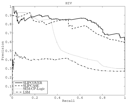
Figure 3: PR curves for HIV.

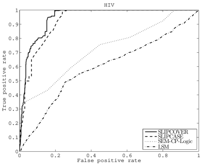
Figure 4: ROC curves for HIV.

The medical literature states that 41L, 215FY and 210W tend to occur together, and that 70R and 219EQ tend to occur together as well. SLIPCASE and LSM find only one of these two connections and the simple MLN learned by LSM may explain its low AUCs. SLIPCOVER instead learns many more clauses where both connections are found, with probabilities larger than the other clauses. The longer learning time with respect to the other systems mainly depends on the theory search phase, since the $TC$ list can contain up to 50 clauses and the final theories have on average 40, so many theory refinement steps are executed.

In the following we show examples of rules that have been learned by the systems, showing only rules expressing the above connections.

SLIPCOVER learned the clauses:

70R:0.950175 :- 219EQ.    ΨΨΨΨΨΨΨΨΨ
41L:0.24228Ψ :- 215FY,Ψ210W.
41L:0.660481 :- 210W.
41L:0.579041 :- 215FY.
219EQ:0.470453 :- 67N,Ψ70R.
219EQ:0.400532 :- 70R.
215FY:0.795429 :- 210W,Ψ219EQ.
215FY:0.486133 :- 41L,Ψ219EQ.
215FY:0.738664 :- 67N,Ψ210W.
215FY:0.492516 :- 67N,Ψ41L.
215FY:0.475875 :- 210W.
215FY:0.924251 :- 41L.
210W:0.425764  :- 41L.

SLIPCASE instead learned:

41L:0.68 :- 215FY.
215FY:0.95 ; 41L:0.05 :- 41L.
210W:0.38 ; 41L:0.25  :- 41L, 215FY.

The clauses learned by SEM-CP-Logic that include the two connections are:

70R:0.30   :-  219EQ.
215FY:0.90 :-  41L.
210W:0.01  :-  215FY.

LSM learned:

1.19 !g41L(a1) v g215FY(a1)
0.28  g41L(a1) v !g215FY(a1)

UW-CSE

The language bias for SLIPCOVER allowed all predicates to appear in the head and in the body of clauses; all except advisedby/2 are background predicates. Moreover, nine modeh facts declare disjunctive heads, three of them are shown in Section 4. These modeh declarations have been defined by looking at the hand crafted theory used for parameter learning in [Bellodi and Riguzzi (2013)]: for each disjunctive clause in the theory, a modeh fact is derived. On this dataset head refinement is applied. The approximate semantics has been used to limit learning time.

The language bias for SLIPCASE allowed advisedby/2 to appear in the head only and all the other predicates in the body only; for this reason we ran it with no depth bound. The input theory was composed of two clauses of the form advisedby(X,Y):0.5.

For LSM, we used the discriminative training algorithm for learning the weights, by specifying advisedby/2 as the only non-evidence predicate, and the MC-SAT algorithm for inference over the test folds, by specifying advisedby/2 as the query predicate.

For Aleph and ALEPH++ExactL1 the same language bias as SLIPCASE was used.

On this dataset SLIPCOVER achieves higher AUCPR and AUCROC than all other systems. This is a difficult dataset, as testified by the low values of areas achieved by all systems, and represents a challenge for structure learning algorithms.

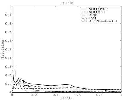
Figure 5: PR curves for UWCSE.

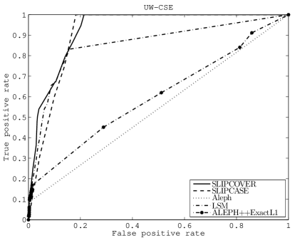
Figure 6: ROC curves for UWCSE.

SLIPCASE learns simple programs composed of a single clause per fold; this also explains the low learning time. In two folds out of five it learns the theory

advisedby(A,B):0.26 :- professor(B), student(A).

An example of a theory learned by LSM is

3.77122  professor(a1) v !advisedBy(a2,a1)
0.03506  !professor(a1) v !advisedBy(a2,a1)
2.27866  student(a1) v !advisedBy(a1,a2)
1.25204  !student(a1) v !advisedBy(a1,a2)
0.64834  hasPosition(a1,a2) v !advisedBy(a3,a1)
1.23174  !advisedBy(a1,a2) v inPhase(a1,a3)

SLIPCOVER learns theories able to better model the domain, at the expense of a longer learning time than SLIPCASE. Examples of clauses are:

advisedby(A,B):0.538049 ; tempadvisedby(A,B):0.261159 :- ta(C,A,D),
                                                         taughtby(C,B,D).
advisedby(A,B):2.97361e-10 :- publication(C,A).
advisedby(A,B):0.0396684 :- publication(C,B),publication(D,A),
                            professor(B),student(A).
advisedby(A,B):0.0223801 :- publication(C,A),publication(D,A),
                            professor(B),student(A).
advisedby(A,B):0.052342 :- professor(B).
hasposition(A,faculty):0.344719; hasposition(A,faculty_adjunct):0.225888;
  hasposition(A,faculty_emeritus):0.14802;
  hasposition(A,faculty_visiting):0.0969946 :- professor(A).
professor(A):0.569775 :- hasposition(A,B).
...

Aleph and ALEPH++ExactL1 mainly differ in the number of learned clauses, while body literals and their ground arguments are essentially the same.
ALEPH++ExactL1 returns more complex MLNs than LSM, and performs slightly better.

WebKB

The language bias for SLIPCOVER and SLIPCASE allowed predicates representing the four categories both in the head and in the body of clauses. Moreover, the body could contain the atom linkTo(_Id,Page1,Page2) (linking two pages) and the atom has(word,Page) where word is a constant representing a word appearing in the pages.
The input theory for SLIPCASE was composed of clauses of the form
<category>Page(Page):0.5., one for each category. The target predicates were treated as closed world in this case, so the corresponding literals in the clauses’ body are resolved only with examples in the mega-examples and not with the other clauses in the theory to limit execution time, therefore $D$ is not relevant. The approximate semantics was used for SLIPCASE to limit the learning time.

LSM failed on this dataset because the weight learning phase quickly exhausted the available memory on our machines (4 GB). This dataset is in fact quite large, with 15 MB input files on average.

For Aleph and ALEPH++ExactL1, we overcame the limit of one target predicate per run by executing Aleph four times on each fold, once for each target predicate. In each run, we removed the target predicate from the modeb declarations to prevent Aleph from testing cyclic theories and going into a loop.

On this dataset SLIPCOVER achieves higher AUCPR and AUCROC than the other systems but the differences are not statistically significant.

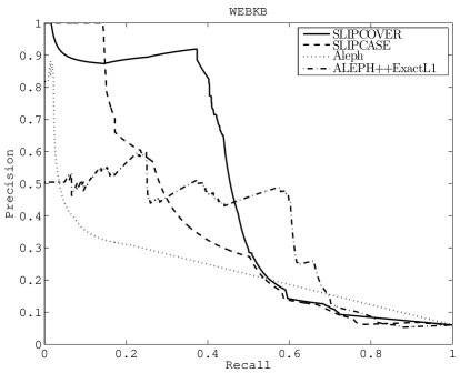
Figure 7: PR curves for WebKB.

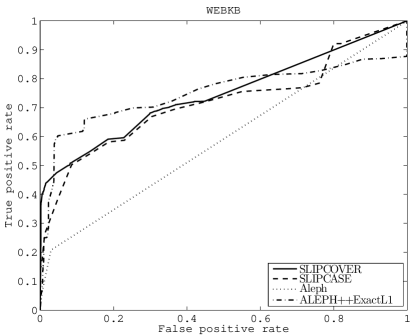
Figure 8: ROC curves for WebKB.

A fragment of a theory learned by SLIPCOVER is:

studentPage(A):0.9398:- linkTo(B,C,A),has(paul,C),has(jame,C),has(link,C).
researchProjectPage(A):0.0321475:- linkTo(B,C,A),has(project,C),
                                   has(depart,C),has(nov,A),has(research,C).
facultyPage(A):0.436275 :- has(professor,A),has(comput,A).
coursePage(A):0.0630934 :- has(date,A),has(gmt,A).

Aleph and ALEPH++ExactL1 learned many more clauses for every target predicate than SLIPCOVER. For coursePage for example ALEPH++ExactL1 learned the clauses

coursePage(A) :-   has(file,A), has(instructor,A), has(mime,A).
coursePage(A) :-   linkTo(B,C,A), has(digit,C), has(theorem,C).
coursePage(A) :-   has(instructor,A), has(thu,A).
coursePage(A) :-   linkTo(B,A,C), has(sourc,C), has(syllabu,A).
coursePage(A) :-   linkTo(B,A,C), has(homework,C), has(syllabu,A).
coursePage(A) :-   has(adapt,A), has(handout,A).
coursePage(A) :-   has(examin,A), has(instructor,A), has(order,A).
coursePage(A) :-   has(instructor,A), has(vector,A).
coursePage(A) :-   linkTo(B,C,A), has(theori,C), has(syllabu,A).
coursePage(A) :-   linkTo(B,C,A), has(zpl,C), has(topic,A).
coursePage(A) :-   linkTo(B,C,A), has(theori,C), has(homework,A).
coursePage(A) :-   has(decemb,A), has(instructor,A), has(structur,A).
coursePage(A) :-   has(apr,A), has(client,A), has(cours,A).
coursePage(A) :-   has(home,A), has(spring,A), has(syllabu,A).
coursePage(A) :-   has(ad,A), has(copyright,A), has(cse,A).
   ...

In this domain SLIPCASE learns fewer and simpler clauses (many with an empty body) for each fold than SLIPCOVER. Moreover, SLIPCASE search strategy generates thousands of refinements for each theory extracted from the beam, while SLIPCOVER beam search generates less than a hundred refinements from each bottom clause, thus achieving a lower learning time.

Mutagenesis

The language bias for SLIPCOVER and SLIPCASE allowed active/1 only in the head, so the depth $D$ was not relevant. For SLIPCASE, we set $\epsilon_{s}=10^{-20}$ and $\delta_{s}=10^{-20}$ to ensure that it performed 10 refinement iterations, so that its execution time was close to that of SLIPCOVER. The input theory for SLIPCASE contained two facts of the form active(D):0.5.

LSM failed on this dataset because the structure learning phase (createrules step) quickly gave a memory allocation error when generating bond/4 groundings.

On this dataset SLIPCOVER achieves higher AUCPR and AUCROC than the other systems, except ALEPH++ExactL1, which achieves the same AUCPR as SLIPCOVER and non statistically significant higher AUCROC. The differences between SLIPCOVER and Aleph are instead statistically significant.

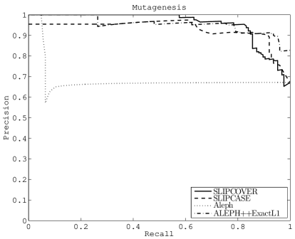
Figure 9: PR curves for Mutagenesis.

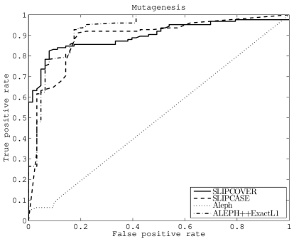
Figure 10: ROC curves for Mutagenesis.

SLIPCOVER learns more complex programs with respect to those learned by SLIPCASE, that contain only two or three clauses for each fold.

[Srinivasan et al. (1994)] (?) report the results of the application of Progol to this dataset. In the following we present the clauses learned by Progol paired with the most similar clauses learned by SLIPCOVER and ALEPH++ExactL1.

Progol learned

active(A) :- atm(A,B,c,10,C),atm(A,D,c,22,E),bond(A,D,B,1).

where a carbon atom c of type 22 is known to be in an aromatic ring.
SLIPCOVER learned

active(A):9.41508e-06 :- bond(A,B,C,7), atm(A,D,c,22,E).ΨΨ
active(A):1.14234e-05 :- benzene(A,B), atm(A,C,c,22,D).

where a bond of type 7 is an aromatic bond and benzene is a 6-membered carbon aromatic ring.

Progol learned

active(A) :- atm(A,B,o,40,C), atm(A,D,n,32,C).

SLIPCOVER instead learned:

active(A):5.3723e-04 :-  bond(A,B,C,7), atm(A,D,n,32,E).

The clause learned by Progol

active(A):-  atm(A,B,c,27,C),bond(A,D,E,1),bond(A,B,E,7).

where a carbon atom c of type 27 merges 2 6-membered aromatic rings, is similar to SLIPCOVER’s

active(A):0.135014 :- benzene(A,B), atm(A,C,c,27,D).

ALEPH++ExactL1 instead learned from all the folds

active(A) :- atm(A,B,c,27,C), lumo(A,D), lteq(D,-1.749).

The Progol clauses

active(A) :- atm(A,B,h,3,0.149).
active(A) :- atm(A,B,h,3,0.144).

mean that a compound with a hydrogen atom $h$ of type 3 with partial charge 0.149 or 0.144 is active. Very similar charge values (0.145) are found by ALEPH++ExactL1.
SLIPCOVER learned

active(A):0.945784 :- atm(A,B,h,3,C),lumo(A,D),D=<-2.242.
active(A):0.01595  :- atm(A,B,h,3,C),logp(A,D),D>=3.26.
active(A):0.00178048 :- benzene(A,B),ring_size_6(A,C),atm(A,D,h,3,E).

SLIPCASE instead learned clauses that relate the drug activity mainly to benzene compounds and energy and charge values; for instance one theory is:

active(A):0.299495 :-  benzene(A,B),lumo(A,C),lteq(C,-1.102),benzene(A,D),
         logp(A,E),lteq(E,6.79),gteq(E,1.49),gteq(C,-2.14),gteq(E,-0.781).
active(A) :-  lumo(A,B),Ψlteq(B,-2.142),lumo(A,C),gteq(B,-3.768),lumo(A,D),
              gteq(C,-3.768).

Hepatitis

The language bias for SLIPCOVER and SLIPCASE allowed type/2 only in the head and all the other predicates in the body of clauses, hence the depth $D$ was not relevant. For SLIPCOVER, $NBC$ was not relevant as only type/2 can appear in the clause heads, and the approximate semantics was necessary to limit learning time. The initial theory for SLIPCASE contained the two facts type(A,type_b):0.5. and type(A,type_c):0.5.

For LSM, we used the discriminative training algorithm for learning the weights, by specifying type/2 as the only non-evidence predicate, and the MC-SAT algorithm for inference over the test fold, by specifying type/2 as the query predicate.

SLIPCOVER achieves significantly higher AUCPR and AUCROC than SLIPCASE and LSM.

Figure 11: PR curves for Hepatitis.

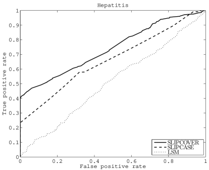
Figure 12: ROC curves for Hepatitis.

Examples of clauses learned by SLIPCOVER are

type(A,type_b):0.344348 :- age(A,age_1).
type(A,type_b):0.403183 :- b_rel11(B,A),Ψfibros(B,C).
type(A,type_c):0.102693 :- b_rel11(B,A),Ψfibros(B,C),b_rel11(D,A),
                           fibros(D,C),age(A,age_6).
type(A,type_c):0.0933488 :- age(A,age_6).
type(A,type_c):0.770442 :- b_rel11(B,A),Ψfibros(B,C),b_rel13(D,A).ΨΨΨΨΨ

Examples of clauses learned by SLIPCASE are

type(A,type_b):0.210837.
type(A,type_c):0.52192 :- b_rel11(B,A),fibros(B,C),b_rel11(D,A),fibros(B,E).
type(A,type_b):0.25556.

LSM long execution time is mainly affected by the createrules phase, where LSM counts the true groundings of all possible unit and binary clauses to find those that are always true in the data: it took 17 hours on all folds; moreover this phase produces only one short clause in every fold.

Table 4: Results of the experiments in terms of the Area Under the PR Curve averaged over the folds. The standard deviations are also shown.

System	HIV	UW-CSE	WebKB	Mutagenesis	Hepatitis
SLIPCOVER	$0.82\pm 0.05$	$0.13\pm 0.02$	$0.47\pm 0.05$	$0.95\pm 0.01$	$0.80\pm 0.01$
SLIPCASE	$0.78\pm 0.05$	$0.03\pm 0.01$	$0.31\pm 0.21$	$0.92\pm 0.08$	$0.71\pm 0.05$
LSM	$0.37\pm 0.03$	$0.07\pm 0.02$	-	-	$0.53\pm 0.04$
SEM-CP-logic	$0.58\pm 0.03$	-	-	-	-
Aleph	-	$0.07\pm 0.02$	$0.15\pm 0.05$	$0.73\pm 0.09$	-
ALEPH++	-	$0.05\pm 0.006$	$0.37\pm 0.16$	$0.95\pm 0.009$	-

Table 5: Results of the experiments in terms of the Area Under the ROC Curve averaged over the folds. The standard deviations are also shown.

System	HIV	UW-CSE	WebKB	Mutagenesis	Hepatitis
SLIPCOVER	$0.95\pm 0.01$	$0.93\pm 0.01$	$0.76\pm 0.01$	$0.89\pm 0.05$	$0.74\pm 0.01$
SLIPCASE	$0.93\pm 0.01$	$0.89\pm 0.03$	$0.70\pm 0.03$	$0.87\pm 0.05$	$0.66\pm 0.06$
LSM	$0.60\pm 0.003$	$0.85\pm 0.21$	-	-	$0.52\pm 0.06$
SEM-CP-Logic	$0.72\pm 0.02$	-	-	-	-
Aleph	-	$0.55\pm 0.001$	$0.59\pm 0.04$	$0.53\pm 0.04$	-
ALEPH++	-	$0.58\pm 0.07$	$0.73\pm 0.27$	$0.90\pm 0.004$	-

Table 6: Normalized Area Under the PR Curve for the high-skew datasets. The skew is the proportion of positive examples on the total testing examples.

System	Mutagenesis	Hepatitis
Skew	0.66	0.5
SLIPCOVER	0.91	0.71
SLIPCASE	0.86	0.58
LSM	-	0.32
Aleph	0.51	-
ALEPH++	0.91	-

Table 7: Execution time in hours of the experiments on all datasets.

System	HIV	UW-CSE	WebKB	Mutagenesis	Hepatitis
SLIPCOVER	0.115	0.067	0.807	20.924	0.036
SLIPCASE	0.010	0.018	5.689	1.426	0.073
LSM	0.003	2.653	-	-	25
Aleph	-	0.079	0.200	0.002	-
ALEPH++	-	0.061	0.320	0.050	-

Table 8: Results of t-test on all datasets relative to AUCPR. p is the p-value of a paired two-tailed t-test between SLIPCOVER and the other systems (significant differences in favor of SLIPCOVER at the 5% level in bold).

System	HIV	UW-CSE	WebKB	Mutagenesis	Hepatitis
SLIPCASE	0.02	0.08	0.24	0.15	0.04
LSM	4.11e-5	0.043	-	-	3.18e-4
SEM-CP-logic	4.82e-5	-	-	-	-
Aleph	-	9.48e-4	0.06	2.84e-4	-
ALEPH++ExactL1	-	0.07	0.57	0.90	-

Table 9: Results of t-test on all datasets relative to AUCROC. p is the p-value of a paired two-tailed t-test between SLIPCOVER and the other systems (significant differences in favor of SLIPCOVER at the 5% level in bold).

System	HIV	UW-CSE	WebKB	Mutagenesis	Hepatitis
SLIPCASE	0.008	0.003	0.14	0.49	0.050
LSM	2.52e-5	0.40	-	-	0.003
SEM-CP-logic	6.16e-5	-	-	-	-
Aleph	-	1.27e-4	0.11	3.93e-5	-
ALEPH++ExactL1	-	6.39e-4	0.88	0.66	-

Overall Remarks

The results in Tables 4 and 5 show that SLIPCOVER achieves larger areas than all the other systems in both AUCPR and AUCROC, for all datasets except Mutagenesis, where ALEPH++ExactL1 behaves slightly better.

SLIPCOVER always outperforms SLIPCASE due to the more advanced language bias and search strategy. We experimented with various SLIPCASE parameters in order to obtain an execution time similar to SLIPCOVER’s and the best match we could find is the one shown. Increasing the number of SLIPCASE iterations often gave a memory error when building BDDs so we could not find a closer match.

Both SLIPCOVER and SLIPCASE always outperform Aleph, showing that a probabilistic ILP system can better model the domain than a purely logical one.

SLIPCOVER’s advantage over LSM lies in a smaller memory footprint, that allows it to be applied in larger domains, and in the effectiveness of the bottom clauses in guiding the search, in comparison with the more complex clause construction process in LSM.

SLIPCOVER improves on ALEPH++ExactL1 by being able to learn disjunctive clauses and by more tightly combining the structure and parameter searches.

The area differences between SLIPCOVER and the other systems are statistically significant in its favor in 17 out of 30 cases at the 5% significance level.

7 Conclusions

We presented SLIPCOVER, an algorithm for learning both the structure and the parameters of Logic Programs with Annotated Disjunctions by performing a beam search in the space of clauses and a greedy search in the space of theories. It can be applied to all languages that are based on the distribution semantics.

The code of SLIPCOVER is available in the source code repository of the development version of Yap and is published at http://sites.unife.it/ml/slipcover together with an user manual.

We tested the algorithm on the real datasets HIV, UW-CSE, WebKB, Mutagenesis and Hepatitis and evaluated its performance - in comparison with the systems SLIPCASE, SEM-CP-logic, LSM, Aleph and ALEPH++ExactL1 - through the AUCPR and AUCROC, and AUCNPR on Mutagenesis and Hepatitis. SLIPCOVER achieves the largest values under all metrics in most cases. This shows that the application of well-known ILP and PLP techniques to the SRL field gives results that are competitive or superior to the state of the art.

In the future we plan to experiment with other search strategies, such as local search in the space of refinements. Moreover, we plan to investigate whether the techniques of LHL and LSM can help improving the performance.

References

- Beerenwinkel et al. (2005) Beerenwinkel, N., Rahnenführer, J., Däumer, M., Hoffmann, D., Kaiser, R., Selbig, J., and Lengauer, T. 2005. Learning multiple evolutionary pathways from cross-sectional data. Journal of Computational Biology 12, 584–598.
- Bellodi and Riguzzi (2011) Bellodi, E. and Riguzzi, F. 2011. Learning the structure of probabilistic logic programs. In Inductive Logic Programming - 21st International Conference (ILP-2011), Revised Selected Papers. Springer, LNCS 7207, 61–75.
- Bellodi and Riguzzi (2012) Bellodi, E. and Riguzzi, F. 2012. Experimentation of an Expectation Maximization algorithm for probabilistic logic programs. Intelligenza Artificiale 8, 3–18.
- Bellodi and Riguzzi (2013) Bellodi, E. and Riguzzi, F. 2013. Expectation Maximization over binary decision diagrams for probabilistic logic programs. Intelligent Data Analysis 17, 343–363.
- Berka et al. (2002) Berka, P., Rauch, J., and Tsumoto, S., Eds. 2002. ECML/PKDD2002 Discovery Challenge.
- Biba et al. (2008) Biba, M., Ferilli, S., and Esposito, F. 2008. Discriminative structure learning of markov logic networks. In Inductive Logic Programming, 18th International Conference (ILP-2008), Proceedings. Springer, LNCS 5194, 59–76.
- Boyd et al. (2012) Boyd, K., Davis, J., Page, D., and Santos Costa, V. 2012. Unachievable region in precision-recall space and its effect on empirical evaluation. In Proceedings of the 29th International Conference on Machine Learning (ICML-2012). icml.cc/Omnipress, 639–646.
- Bragaglia and Riguzzi (2011) Bragaglia, S. and Riguzzi, F. 2011. Approximate inference for Logic Programs with Annotated Disjunctions. In Inductive Logic Programming, 20th International Conference (ILP-2010), Revised Papers. Springer, LNCS 6489, 30–37.
- Craven and Slattery (2001) Craven, M. and Slattery, S. 2001. Relational learning with statistical predicate invention: better models for hypertext. Machine Learning 43, 97–119.
- Dantsin (1991) Dantsin, E. 1991. Probabilistic Logic Programs and their semantics. In Russian Conference on Logic Programming (RCLP-1991). Springer, LNCS 592, 152–164.
- Darwiche (2004) Darwiche, A. 2004. New advances in compiling CNF into Decomposable Negation Normal Form. In Proceedings of the 16th Eureopean Conference on Artificial Intelligence (ECAI-2004). IOS Press, 328–332.
- Davis and Goadrich (2006) Davis, J. and Goadrich, M. 2006. The relationship between Precision-Recall and ROC curves. In Machine Learning, Proceedings of the 23rd International Conference (ICML-2006). ACM, ACM International Conference Proceeding Series 148, 233–240.
- De Raedt et al. (2008) De Raedt, L., Demoen, B., Fierens, D., Gutmann, B., Janssens, G., Kimmig, A., Landwehr, N., Mantadelis, T., Meert, W., Rocha, R., Santos Costa, V., Thon, I., and Vennekens, J. 2008. Towards digesting the alphabet-soup of statistical relational learning. In 1st Workshop on Probabilistic Programming: Universal Languages, Systems and Applications (NIPS*2008).
- De Raedt et al. (2008) De Raedt, L., Kersting, K., Kimmig, A., Revoredo, K., and Toivonen, H. 2008. Compressing probabilistic Prolog programs. Machine Learning 70, 151–168.
- De Raedt et al. (2007) De Raedt, L., Kimmig, A., and Toivonen, H. 2007. ProbLog: A Probabilistic Prolog and its application in link discovery. In Proceedings of the 20th International Joint Conference on Artificial Intelligence (IJCAI-2007). AAAI Press, 2462–2467.
- De Raedt and Thon (2010) De Raedt, L. and Thon, I. 2010. Probabilistic rule learning. In Inductive Logic Programming - 20th International Conference (ILP-2010), Revised Papers. Springer, LNCS 7207, 47–58.
- Fawcett (2006) Fawcett, T. 2006. An introduction to ROC analysis. Pattern Recognition Letters 27, 861–874.
- Friedman (1998) Friedman, N. 1998. The Bayesian Structural EM algorithm. In Proceedings of the 14th Conference on Uncertainty in Artificial Intelligence (UAI’98). Morgan Kaufmann, 129–138.
- Fuhr (2000) Fuhr, N. 2000. Probabilistic datalog: Implementing logical information retrieval for advanced applications. Journal of the American Society for Information Science 51, 95–110.
- Getoor et al. (2007) Getoor, L., Friedman, N., Koller, D., Pfeffer, A., and Taskar, B. 2007. Probabilistic Relational Models. In Introduction to Statistical Relational Learning, L. Getoor and B. Taskar, Eds. MIT Press.
- Gutmann et al. (2008) Gutmann, B., Kimmig, A., Kersting, K., and De Raedt, L. 2008. Parameter learning in probabilistic databases: A least squares approach. In Machine Learning and Knowledge Discovery in Databases - European Conference (ECML/PKDD-2008), Proceedings, Part I. Springer, LNCS 5211, 473–488.
- Gutmann et al. (2010) Gutmann, B., Kimmig, A., Kersting, K., and De Raedt, L. 2010. Parameter estimation in ProbLog from annotated queries. Tech. Rep. CW 583, KU Leuven.
- Gutmann et al. (2011) Gutmann, B., Thon, I., and De Raedt, L. 2011. Learning the parameters of probabilistic logic programs from interpretations. In Machine Learning and Knowledge Discovery in Databases - European Conference (ECML/PKDD-2011), Proceedings, Part I. Springer, LNCS 6911, 581–596.
- Huynh and Mooney (2008) Huynh, T. N. and Mooney, R. J. 2008. Discriminative structure and parameter learning for markov logic networks. In Machine Learning, Proceedings of the 25th International Conference (ICML-2008). ACM, ACM International Conference Proceeding Series 307, 416–423.
- Inoue et al. (2009) Inoue, K., Sato, T., Ishihata, M., Kameya, Y., and Nabeshima, H. 2009. Evaluating abductive hypotheses using an EM algorithm on BDDs. In Proceedings of the 21st International Joint Conference on Artificial Intelligence (IJCAI-2009). Morgan Kaufmann Publishers Inc., 810–815.
- Ishihata et al. (2008a) Ishihata, M., Kameya, Y., Sato, T., and Minato, S. 2008a. Propositionalizing the EM algorithm by BDDs. In 18th International Conference on Inductive Logic Programming (ILP-2008), Late Breaking Papers. 44–49.
- Ishihata et al. (2008b) Ishihata, M., Kameya, Y., Sato, T., and Minato, S. 2008b. Propositionalizing the EM algorithm by BDDs. Tech. Rep. TR08-0004, Dep. of Computer Science, Tokyo Institute of Technology.
- Ishihata et al. (2011) Ishihata, M., Sato, T., and ichi Minato, S. 2011. Compiling bayesian networks for parameter learning based on Shared BDDs. In AI 2011: Advances in Artificial Intelligence, 24th Australasian Joint Conference, Proceedings. Springer, LNCS 7106, 203–212.
- Kersting and De Raedt (2008) Kersting, K. and De Raedt, L. 2008. Basic principles of learning Bayesian Logic Programs. In Probabilistic Inductive Logic Programming, L. De Raedt, P. Frasconi, K. Kersting, and S. Muggleton, Eds. Springer, LNCS 4911, 189–221.
- Khosravi et al. (2012) Khosravi, H., Schulte, O., Hu, J., and Gao, T. 2012. Learning compact Markov logic networks with decision trees. Machine Learning 89, 257–277.
- Kimmig et al. (2011) Kimmig, A., Demoen, B., De Raedt, L., Santos Costa, V., and Rocha, R. 2011. On the implementation of the probabilistic logic programming language ProbLog. Theory and Practice of Logic Programming 11, 235–262.
- Kok and Domingos (2005) Kok, S. and Domingos, P. 2005. Learning the structure of Markov logic networks. In Machine Learning, Proceedings of the 22nd International Conference (ICML-2005). ACM, ACM International Conference Proceeding Series 119, 441–448.
- Kok and Domingos (2009) Kok, S. and Domingos, P. 2009. Learning Markov logic network structure via hypergraph lifting. In Proceedings of the 26th Annual International Conference on Machine Learning (ICML-2009). ACM, ACM International Conference Proceeding Series 382, 505–512.
- Kok and Domingos (2010) Kok, S. and Domingos, P. 2010. Learning Markov Logic Networks using structural motifs. In Proceedings of the 27th International Conference on Machine Learning (ICML-2010). Omnipress, 551–558.
- Lowd and Domingos (2007) Lowd, D. and Domingos, P. 2007. Efficient weight learning for Markov logic networks. In Proceedings of the 18th European Conference on Machine Learning (ECML-2007). Springer, LNCS 4702, 200–211.
- Meert et al. (2008) Meert, W., Struyf, J., and Blockeel, H. 2008. Learning ground CP-Logic theories by leveraging Bayesian network learning techniques. Fundamenta Informaticae 89, 131–160.