* See pages - of An_Electronic_Quantum_Eraser_Main

An Electronic Quantum Eraser
Supplemental Material

Detailed treatment

The Electronic Mach-Zehnder Interferometer

Manipulating the geometry of the 2DEG, either by permanent etching or by electrostatic depletion, provides control over the shape of the edge states. In particular, bringing two opposite edge states close together over a short distance, in a structure known as a quantum point contact (QPC), allows controlled tunneling between the edges.

The properties of a QPC, which is the electronic equivalent of an optical beam splitter, are described by a scattering matrix

$$S=\begin{pmatrix}r&it\\ it&r\end{pmatrix}$$

where ${t,r}\in\mathbb{R},\left|{r}\right|^{2}+\left|{t}\right|^{2}=1$ are the QPC’s transmission and reflection amplitudes, respectively. The scattering matrix links the amplitudes of the two states entering the QPC to those of the two states exiting it.

An electronic Mach-Zehnder interferometer (MZI) is composed of two QPCs in succession The first QPC puts an impinging electron into a superpositions of being transmitted and being reflected. The two paths are recombined at the second QPC, the resulting interference reflecting the phase difference between the two paths taken. The accumulated phase $\mathrm{\varphi}$ depends on the magnetic flux enclosed by the two paths.

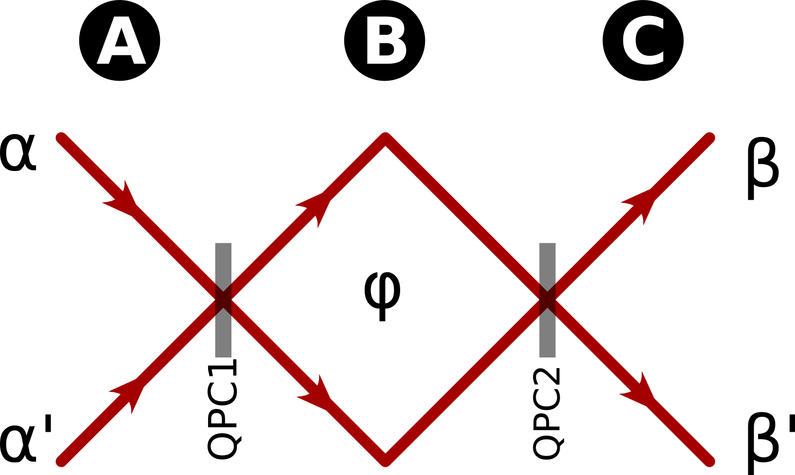
Figure 1: An electronic Mach-Zehnder interferometer (MZI). The electronic MZI is the electronic counterpart of the optical MZI, where two potential barriers take the role of bean splitters. An electron emanating from a source contact impinges upon the first barrier (Region A) and is put into a superposition of being in the lower and upper arms (Region B). The two arms reunite at the second barrier, allowing the two states to interfere. The current at each drain contact depends on the phase difference between the two paths (Region C).

Let us denote the portions before, between and after the two QPCs with A,B, and C, respectively. The Hilbert space before the QPCs (region A) is spanned by the two source states

$$\left|{\alpha}\right\rangle\equiv\begin{pmatrix}{1}\\ {0}\end{pmatrix},\left|{\alpha^{\prime}}\right\rangle\equiv\begin{pmatrix}{0}\\ {1}\end{pmatrix};$$

The intermediate region is spanned by the upper and lower path states,

$$\left|{\uparrow}\right\rangle\equiv\begin{pmatrix}{1}\\ {0}\end{pmatrix},\left|{\downarrow}\right\rangle\equiv\begin{pmatrix}{0}\\ {1}\end{pmatrix};$$

The region after the QPCs is spanned by the detector states

$$\left|{\beta}\right\rangle\equiv\begin{pmatrix}{1}\\ {0}\end{pmatrix},\left|{\beta^{\prime}}\right\rangle\equiv\begin{pmatrix}{0}\\ {1}\end{pmatrix}.$$

In all of our experiments the initial state of the system is $\mathrm{\left|{\alpha}\right\rangle}$ and the final state is $\mathrm{\left|{\beta}\right\rangle}$.

To obtain the system’s state between the QPCs (region B) we apply SQPC1’s scattering matrix to the initial state:

$$\left|{S_{B}}\right\rangle=S_{1}\left|{\alpha}\right\rangle=\begin{pmatrix}{r_{1}}\\ {-it_{1}}\end{pmatrix}.$$

In order to get state of the system after interfering at SQPC2 (region C) we apply an operator accounting for the AB phase $\mathrm{\varphi_{S}}$ accumulated in region B,

$$S_{\varphi_{S}}=\begin{pmatrix}e^{i\varphi_{S}}&0\\ 0&1\end{pmatrix},$$

and the scattering matrix for SQPC2:

$$\left|{S_{C}}\right\rangle=S_{2}S_{\varphi_{S}}\left|{S_{B}}\right\rangle=\begin{pmatrix}{r_{1}r_{2}e^{i\varphi_{S}}-t_{1}t_{2}}\\ {ir_{1}t_{2}e^{i\varphi_{S}}+it_{1}r_{2}}\end{pmatrix}.$$

The overall probability for an electron to be transmitted into state $\mathrm{\left|{\beta}\right\rangle}$ is simply

$$P(\beta)=\left|{\left\langle{\beta}\right|\left.{S_{C}}\right\rangle}\right|^{2}=T_{0}-T_{1}\cos(\varphi_{S})$$

where $T_{0}=\left(t_{1}t_{2}\right)^{2}+\left(r_{1}r_{2}\right)^{2},T_{1}=2t_{1}t_{2}r_{1}r_{2}$. Since consecutive tunneling events of two electrons are statically independent, the total current at $\mathrm{\beta}$ depends linearly on the input current: $I_{\beta}=P(\beta)I_{\alpha}$. The visibility of the MZI is defined as

$$v_{\beta}=\frac{max(I_{\beta})-min(I_{\beta})}{max(I_{\beta})+min(I_{\beta})}=\xi\frac{T_{1}}{T_{0}}$$

where $0\leq\xi\leq 1$ is a phenomenological constant describing the loss of visibility due to unwanted dephasing by the environment.

Entanglement and Quantum Erasure

Entanglement and dephasing

Consider a complex of two MZIs formed using different edge channels and positioned such that the two reflected arms each MZI are in close proximity. Electrons passing simultaneously in the neighboring paths will interact electrically, rendering the two MZI entangled. We make an arbitrary choice to call one of these MZI the system, S, and the other the detector, D. Each is sectioned, as above, into the region before, in-between, and after the QPCs (regions A,B,C). The electrostatic interaction, when it takes place, changes the detector electron’s trajectory, adding $\mathrm{\gamma}$ to its phase. That is, if the system is $\mathrm{\left|{\downarrow}\right\rangle_{S}}$ the state of the detector in region B would be

$$\left|{0}\right\rangle_{D}=S_{3}\left|{\alpha}\right\rangle_{D}=\begin{pmatrix}{r_{3}}\\ {it_{3}}\end{pmatrix}_{D}$$

and if the system is $\mathrm{\left|{\uparrow}\right\rangle_{S}}$ the state of the detector would be

$$\left|{\gamma}\right\rangle_{D}=S_{\gamma}S_{3}\left|{\alpha}\right\rangle_{D}=\begin{pmatrix}{r_{3}e^{i\gamma}}\\ {it_{3}}\end{pmatrix}_{D}.$$

The system-detector complex is in an entangled state, which is a superposition of the above mentioned options:

$$\left|{\Psi_{B}}\right\rangle=r_{1}\left|{\downarrow}\right\rangle_{S}\otimes\left|{0}\right\rangle_{D}+it_{1}\left|{\uparrow_{S}}\right\rangle\otimes\left|{\gamma}\right\rangle_{D}.$$

The transmission probability is found in the same manner as for a single MZI. We advance the state $\mathrm{\left|{\Psi_{B}}\right\rangle}$ to region C:

$$\left|{\Psi_{C}}\right\rangle =S_{4}S_{\varphi_{D}}S_{2}S_{\varphi_{S}}\left|{\Psi_{B}}\right\rangle$$

$$=\begin{pmatrix}{r_{1}r_{2}e^{i\varphi_{S}}}\\ {ir_{1}t_{2}e^{i\varphi_{S}}}\end{pmatrix}_{S}\otimes\begin{pmatrix}{r_{3}r_{4}e^{i(\varphi_{D}+\gamma)}-t_{3}t_{4}}\\ {ir_{3}t_{4}e^{i(\varphi_{D}+\gamma)}+it_{3}r_{4}}\end{pmatrix}_{D}+$$

$$\quad\begin{pmatrix}{-t_{1}t_{2}}\\ {it_{1}r_{2}}\end{pmatrix}_{S}\otimes\begin{pmatrix}{r_{3}r_{4}e^{i\varphi_{D}}-t_{3}t_{4}}\\ {ir_{3}t_{4}e^{i\varphi_{D}}+it_{3}r_{4}}\end{pmatrix}_{D}.$$

The transmission of the system MZI is altered by the interaction:

$$P(\beta_{S}) =\left|{\left\langle{\beta_{S}}\right|\left.{\Psi_{C}}\right\rangle}\right|^{2}=T_{0,S}-T_{1,S}Re\left(e^{i\varphi_{S}}\left\langle{0}\right|\left.{\gamma}\right\rangle_{D}\right)$$

$$=T_{0,S}-T_{1,S}\left({r_{3}}^{2}\cos(\varphi_{S}+\gamma)+{t_{3}}^{2}\cos(\varphi_{S})\right)$$

where $T_{0,S}=\left(t_{1}t_{2}\right)^{2}+\left(r_{1}r_{2}\right)^{2},T_{1,S}=2t_{1}t_{2}r_{1}r_{2}$. Not surprisingly, the transmission of the detector is similar:

$$P(\beta_{D})=\left|{\left\langle{\beta_{D}}\right|\left.{\Psi_{C}}\right\rangle}\right|^{2}=T_{0,D}-2T_{1,D}\left({r_{1}}^{2}\cos(\varphi_{D}+\gamma)+{t_{1}}^{2}\cos(\varphi_{D})\right)$$

where $T_{0,D}=\left(t_{3}t_{4}\right)^{2}+\left(r_{3}r_{4}\right)^{2},T_{1,S}=2t_{3}t_{4}r_{3}r_{4}$.

Quantum Erasure and Recovery

The joint probability for two events, that is the probability for both to happen, is found by taking the expectation value for the product of their projection operators. Specifically, the joint probability of detecting electrons at $\mathrm{\beta_{S}}$ and $\mathrm{\beta_{D}}$ is

$$P(\beta_{S}\beta_{D}) =\langle\beta_{S}\beta_{D}\rangle=\left|{\left\langle{\Psi}\right|\left.{\beta_{S}}\right\rangle\left\langle{\beta_{S}}\right|\left.{\beta_{D}}\right\rangle\left\langle{\beta_{D}}\right|\left.{\Psi}\right\rangle}\right|$$

$$=\left|{\left\langle{\beta_{D}}\right|\beta_{S}\left|{\Psi}\right\rangle}\right|^{2}.$$

If the events at the drains are independent the joint-probability is simply $P(\beta_{S}\beta_{D})=P(\beta_{S})P(\beta_{D})$. We are interested in the reduced joint probability, $P(\Delta\beta_{S}\Delta\beta_{D})=P(\beta_{S}\beta_{D})-P(\beta_{S})P(\beta_{D})$, which is the non-trivial correlation between the two drains, originating in the system-detector entanglement.

In the general case, the expression for the reduced joint probability is a rather cumbersome one

$$P(\Delta\beta_{S}\Delta\beta_{D}) =P(\beta_{S}\beta_{D})-P(\beta_{S})P(\beta_{D})=$$

$$\quad\left|{r_{1}r_{2}e^{i\varphi_{S}}\left(r_{3}r_{4}e^{i(\varphi_{S}+\gamma)}-t_{3}t_{4}\right)-t_{1}t_{2}\left(r_{3}r_{4}e^{i\varphi_{S}}-t_{3}t_{4}\right)}\right|^{2}-$$

$$\quad\left[(t_{1}t_{2})^{2}+(r_{1}r_{2})^{2}-2r_{1}r_{2}t_{1}t_{2}\left({r_{3}}^{2}\cos(\varphi_{S}+\gamma)+{t_{3}}^{2}\cos(\varphi_{S})\right)\right]\times$$

$$\quad\left[(t_{3}t_{4})^{2}+(r_{3}r_{4})^{2}-2r_{3}r_{4}t_{3}t_{4}\left({r_{1}}^{2}\cos(\varphi_{D}+\gamma)+{t_{1}}^{2}\cos(\varphi_{D})\right)\right].$$

But for symmetrically tuned MZIs ($t_{i},r_{i}=\tfrac{1}{\sqrt{2}},i=1\ldots 4$), the above reduces to

$$P(\Delta\beta_{S}\Delta\beta_{D})=\tfrac{1}{4}\cos\left(\varphi_{S}+\frac{\gamma}{2}\right)\cos\left(\varphi_{D}+\frac{\gamma}{2}\right)\sin^{2}\left(\frac{\gamma}{2}\right).$$

The autocorrelations $\mathrm{(P(\Delta\beta^{2})}$ can be obtained in a similar manner, taking note that $P(\beta\beta)=P(\beta)$:

$$P(\Delta\beta_{j}\Delta\beta_{j})=P(\beta_{j})\left(1-P(\beta_{j})\right),j=S,D$$

which determines the power spectral density at the MZI drain:

$$S_{\beta} =2eI_{\alpha}P(\beta)\left(1-P(\beta)\right)$$

$$=T_{0}(1-T_{0})+T_{1}(2T_{0}-1)\xi\cos(\varphi)-{T_{1}}^{2}\xi^{2}\cos^{2}(\varphi).$$

Technical considerations

Biasing limitation

The currents used in our setup (and similar setups) were limited to about 1 nA per edge channel. Higher currents were observed to tunneling to adjacent co-propagating edge channels. Note that even for smaller currents and counter-propagating edge channel we observed a minute signal transfer (<1%) between the edges at high-frequency, probably due to capacitive coupling. In addition, most QPCs show bias dependent transmission profile, especially at higher voltage biases. In our experiment we took care to work in a regime where no significant current tunneling occurred and QPC transmission was not bias dependent.

Random phase noise

During our experiment we observed that the interference of a MZI constructed using the innermost edge channel is plagued by random phase noise: both QPCs forming the MZI showed stable transmission, the interference had high visibility, comparable to other edges channels, but the AB phase jumped randomly at a rate of about 1 Hz. Our understanding is that these jumps originate from random charging and discharging events (e.g. in quantum dots formed in the bulk due to crystal defects) in the vicinity of the MZI, which is highly sensitive to charge fluctuations, especially to those occurring in nearly isolated quantum dots [1]. However, when interfering the outer edge channels, the innermost edge channel engulfs the interfering edge, shielding it from the above-mentioned charge fluctuations, thus eliminating the random phase noise. For this reason, it was essential in our experiment to let the inner edge pass through the interaction region, even at the expense of weakening the interaction, both due to increasing the distance between the interacting edges and the shielding by the inner edge channel.

MZI lobe structure

The MZI transmission is energy dependent in a non-trivial way [2], declining as the source-drain bias is increased; when it reaches zero, it recovers, with a $\pi$ phase shift and then declines again, forming a so-called ’lobe pattern’. For a DC, the overall AB oscillation amplitude is set by a summation on all energies, up to the applied voltage bias. Therefore, the maximal visibility is obtained at the voltage bias for which the energy-dependent transmission reaches zero. For our MZI this occurred at about 6.5 $\mathrm{\mu eV}$, which implies a current of 0.5 nA.

Other configurations examined

We attempted several different configurations in hopes of increasing the maximal interaction between the two MZI.

Gate separated double MZI

One approach form two MZI where the interacting paths are separated by a very thin (50 nm) metallic gate. We hoped that the reduced distance, and the absence of shielding by the inner edges will boost the interaction. Although the MZI showed very high visibility (>90%), the interaction was too small to observe. We attribute this to the separating gate’s ability to screen the two MZI from each other.

Figure 2: An alternative EQE setup. The interacting paths are separated by a thin surface gate, in hopes of achieving stronger interaction. However, the gate seems to be very efficient in shielding the two MZI from each other.

Co-propagating edges double MZI

Another approach was to construct the two MZI using different, co-propagating edges. Since the co-propagating edges are very close and there is nothing to screen them from each other, we expected to observe a strong interaction. For this purpose we filling factor 3 of the IQHE: the outermost edge formed one MZI, the middle edge formed another MZI and the innermost edge shielded the two MZI random charge fluctuations in the bulk (see above). Indeed, this setup achieved strong interaction between the two MZI, gaining full dephasing for currents of 1.0 nA per edge channel. However, it turned out that the tunneling between co-propagating edges was large to the extent of preventing useful measurements. The tunneling occurred only when the MZI were tuned, hinting to some resonative source for this behavior.

References

• [1] EΒ Weisz, HKΒ Choi, MΒ Heiblum, Yuval Gefen, VΒ Umansky, and DΒ Mahalu. Controlled dephasing of an electron interferometer with a path detector at equilibrium. Phys. Rev. Lett., 109(25):250401, 2012.
• [2] I.Β Neder, M.Β Heiblum, Y.Β Levinson, D.Β Mahalu, and V.Β Umansky. Unexpected behavior in a two path electron interferometer. Phys. Rev. Lett., 96, 2006.