Universality and scaling in the $N$-body sector of Efimov physics

Abstract

Universal behaviour has been found inside the window of Efimov physics for systems with $N=4,5,6$ particles. Efimov physics refers to the emergence of a number of three-body states in systems of identical bosons interacting via a short-range interaction becoming infinite at the verge of binding two particles. These Efimov states display a discrete scale invariance symmetry, with the scaling factor independent of the microscopic interaction. Their energies in the limit of zero-range interaction can be parametrized, as a function of the scattering length, by a universal function. We have found, using the form of finite-range scaling introduced in [A. Kievsky and M. Gattobigio, Phys. Rev A 87, 052719 (2013)], that the same universal function can be used to parametrize the ground- and excited-energy of $N\leq 6$ systems inside the Efimov-physics window. Moreover, we show that the same finite-scale analysis reconciles experimental measurements of three-body binding energies with the universal theory.

Universality is one of the concepts that have attracted physicists along the years. Different systems, having even different energy scales, share common behaviours. The most celebrated example of universality comes from the investigation of critical phenomena Wilson (1983); Fisher (1998): at the critical point, materials that are governed by different microscopic interactions share the same macroscopic laws, for instance the same critical exponents. The theoretical framework to understand universality has been provided by the renormalization group (RG); the critical point is mapped onto a fixed point of a dynamical system, the RG flow, whose phase space is represented by Hamiltonians. At the critical point the systems have scale-invariant (SI) symmetry, forcing all of the observables to be exponential functions of the control parameter. A consequence of SI symmetry is the scaling of the observables: for different materials, in the same class of universality, a selected observable can be represented as a function of the control parameter and, provided that both the observable and the control parameter are scaled by some material-dependent factor, all representations collapse onto a single universal curve Stanley (1999).

More recently, a new kind of universality has captured the interest of physicists, namely the Efimov effect Efimov (1970, 1971). A system of three identical bosons interacting via two-body short-range interaction whose strength is tuned, by scientists or by nature, to the verge of binding the two particle subsystem, exhibits the appearance of an infinite tower of three-particle bound states, whose energies accumulate to zero. Moreover, the ratio between the energies of two consecutive states is constant and independent of the very nature of the interaction; this last property points out to the emergence of a discrete scale invariance (DSI) symmetry (for a complete review, see Ref. Braaten and Hammer (2006)).

Even this example of universality has found in the RG its theoretical framework. Systems sharing Efimov effect are mapped onto a limit cycle of the RG flow, where they manifest the emergence of DSI. In turn, DSI implies that all of the observables are log-periodic function of the control parameter Sornette (1998), and this property is what characterizes the Efimov physics, of which Efimov effect is an example. The limit cycle implies the emergence of a new dimensional quantity, which in the case of Efimov physics is known as the three-body parameter. Strictly speaking, the DSI is an exact symmetry for systems with zero-range interaction, or equivalently in the scaling limit; for real systems, which posses an interaction with finite range $r_{0}$, there are deviations from DSI called finite-range effects.

Atomic physics, and more precisely experiments using ultracold-alkali atoms, has recently (re)sparked the interest in Efimov physics Kraemer et al. (2006). At present, several different experimental groups have observed the Efimov effect in alkali systems Ferlaino et al. (2011); Machtey et al. (2012); Roy et al. (2013); Dyke et al. (2013), where the key point has been the scientists’ ability to change the two-body scattering length $a$ by means of Fano-Feshbach resonances. In fact, the theory predicts how observables change as a function of the control parameter, $\kappa_{*}a$, which is proportional to the scattering length, making the tuning of $a$ crucial to test theory’s predictions. In particular, the Efimov equation for the three-body binding energies $E_{3}^{n}$ can be expressed in a parametric form as follow Braaten and Hammer (2006)

$$\begin{gathered}E_{3}^{n}/(\hbar^{2}/ma^{2})=\tan^{2}\xi\\ \kappa_{*}a=\text{e}^{(n-n^{*})\pi/s_{0}}\frac{\text{e}^{-\Delta(\xi)/2s_{0}}}{\cos\xi}\,,\end{gathered}$$ (1)

with $\Delta(\xi)$ a universal function whose parametrization can be found in Ref. Braaten and Hammer (2006), $s_{0}=1.00624$, and $\kappa_{*}$ the emergent three-body parameter which gives the energy $\hbar^{2}\kappa_{*}^{2}/m$ for $n=n^{*}$ at the unitary limit $1/a=0$.

The ability of tuning $a$, has allowed the different experimental groups to measure the value of the scattering length $a_{-}$ at which the three-body bound state disappears into the continuum ($\xi\rightarrow-\pi$). From Eq. (1) we see that measuring $a_{-}=-\text{e}^{-\Delta(\pi)/2s_{0}}/\kappa_{*}\approx-1.56/\kappa_{*}$ Esry et al. (1999); Bedaque et al. (2000), is a way to measure the three-body parameter $\kappa_{*}$, which in principle should be different for different systems. However, it has been experimental found Ferlaino et al. (2011); Machtey et al. (2012); Roy et al. (2013); Dyke et al. (2013), and theoretically justified Wang et al. (2012); Naidon et al. (2012), that in the class of alkali atoms $a_{-}/\ell\approx-9.5$, with $\ell$ the van der Waals length; a universality inside universality. Recently the same behavior has been seen in a gas of $\,{}^{4}$He atoms Knoop et al. (2012).

Eq. (1), as well as the parametrization of $\Delta(\xi)$ have been derived in the scaling limit, where the DSI is exact. Experiments and calculations made for real systems deal with finite-range interactions, $r_{0}\neq 0$, and for this reason finite-range corrections have to be considered Efimov (1991); Thøgersen et al. (2008); D’Incao et al. (2009); Platter et al. (2009). In a recent paper Kievsky and Gattobigio (2013), the authors have observed in which manner finite-range corrections manifest in numerical calculations using potential models:

(i) There are corrections coming from the two-body sector which can be taken into account by substituting $a_{B}$ for $a$, defined by $E_{2}=\hbar^{2}/ma_{B}^{2}$, with $E_{2}$ the two-body binding energy if $a>0$, or the two-body virtual-state energy in the opposite case, $a<0$ Ma (1953). One simple way to obtain the virtual-state energy is looking for the poles of the two-body S-matrix using a Padè approximation, as shown in Ref. Rakityansky et al. (2007). It should be noticed that in the zero-range limit $a_{B}\rightarrow a$.

(ii) The finite-range corrections enter as a shift in the control parameter $\kappa_{*}a_{B}$. The value of the shift depends on the observable under investigation.

For instance, in the case of three-body binding energies, (i) and (ii) applied to Eq. (1) give

$$\begin{gathered}E_{3}^{n}/E_{2}=\tan^{2}\xi\\ \kappa^{3}_{n}a_{B}+\Gamma_{n}^{3}=\frac{\text{e}^{-\Delta(\xi)/2s_{0}}}{\cos\xi}\,,\end{gathered}$$ (2)

where we have defined $\kappa_{n}^{3}=\kappa_{*}\text{e}^{(n-n^{*})\pi/s_{0}}$, and introduced the shifts $\Gamma_{n}^{3}$. In Ref. Kievsky and Gattobigio (2013) the authors have shown that this type of correction appears in the energy spectrum, in atom-dimer scattering length and in the effective range function of three boson atoms. Moreover, in Ref. Garrido et al. (2013) it has been shown that the shift appears in recombination rate of three atoms close to threshold too.

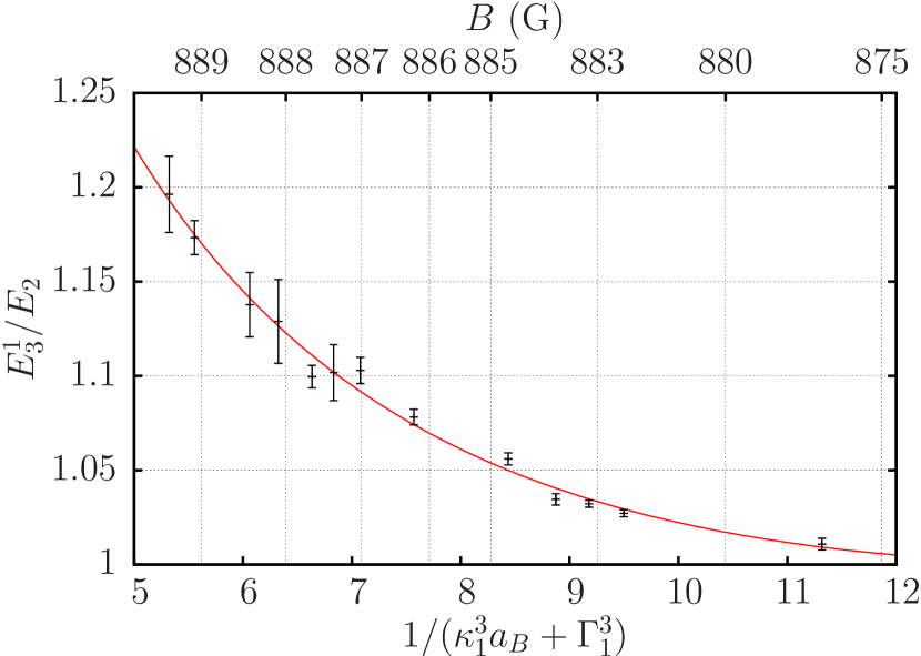
Figure 1: (color online). The experimental data on $\ {}^{7}$Li Machtey et al. (2012), in the form of ratio between the three-body binding energy $E_{3}^{1}$ and the two-body binding energy $E_{2}$, as a function of $1/(\kappa_{1}^{3}a_{B}+\Gamma_{1}^{3})$ with the values of the three-body parameters given in the text. The solid curve represents the prediction of the universal function, Eq. (2). In the upper abscissa the magnetic field from Ref. Gross et al. (2011) is given.

Our finite-range analysis can be applied to describe experimental data. In Fig. 1 we report the experimental three-body binding energies measured in $\ {}^{7}$Li Machtey et al. (2012) and for reference the corresponding magnetic field Gross et al. (2011). Using Eq. (2) with the values of the two three-body parameters $\Gamma_{1}^{3}=4.95\times 10^{-2}$ and $\kappa^{3}_{1}=1.61\times 10^{-4}\,a_{0}$ the experimental point collapse on the universal curve (solid line). A more extended analysis is underway.

To explain the origin of this form of finite-range correction, we refer to the original derivation Efimov (1971) of Eq. (1) and to the parametrization of the universal phase $\Delta(\xi)$, for instance in Ref. Braaten and Hammer (2006). In the zero-range limit $r_{0}=0$ the adiabatic approximation is exact, and the three-body problem is equivalent to a single Schrödinger equation in a scale-invariant $1/R^{2}$ potential, where $R^{2}\propto r_{12}^{2}+r_{13}^{2}+r^{2}_{23}$ is the hyperradius; Eq. (1) has been derived by matching the scale-invariant phase shift $\Delta(\xi)$ originating from the long-range physics to the scaling-violating phase shift originating from the short-range physics (see Eq.(193) of Ref. Braaten and Hammer (2006)). The short-range physics can be encoded in a scale-violating momentum $\Lambda_{0}$, see Eq. (147) of Braaten and Hammer (2006), and the parametrization, for a zero-range theory, of $\Delta(\xi)$ is such that $\Lambda_{0}=\kappa_{*}$. Now, when we consider a finite-range system, $r_{0}\neq 0$, the lowest adiabatic potential is coupled to the other adiabatic potentials: for instance, it has been demonstrated by Efimov Efimov (1991) that the coupling can be taken into account by a correction $\sim r_{0}/R^{3}$ on the lowest potential. This means that, keeping the same parametrization of $\Delta(\xi)$, the relation between $\Lambda_{0}$ and $\kappa_{*}$ is modified, and at the first order we can expect

$$\Lambda_{0}\simeq\kappa_{*}\left(1+{\cal A}\,\frac{r_{0}}{a_{B}}\right)\,,$$ (3)

which gives the shift $\Gamma^{3}_{n^{*}}={\cal A}\,\kappa_{*}r_{0}$. The constant ${\cal A}$ is expected to take natural values.

In this work we extend the application of the modifications to the zero-range theory in order to analyze the ground- and excited-binding energy of $N$-body systems obtained by numerical calculations inside the window of Efimov physics. The Efimov effect is strictly related to the $N=3$ system, but one can try to investigate if and how Efimov physics affects $N>3$ sectors. Some seminal-theoretical studies Platter et al. (2004); von Stecher et al. (2009); Deltuva (2013), and subsequent experimental investigation Ferlaino et al. (2009), have demonstrated that for each trimer belonging to the Efimov tower there are two attached four-body states. This property has also been observed in $N=5,6$ Gattobigio et al. (2011a); von Stecher (2011); Gattobigio et al. (2012): there are two attached five-body states to the four-body ground state and there are two attached six-body states to the five-body ground state. These states have been characterized by measuring ratios between energies close to the unitary limit, and these ratios have been found to be universal. Moreover, their stability has been analyzed along the Efimov plane in wide region of the angle $\xi$ Gattobigio et al. (2013).

We want to make a step forward showing that the three-body equation, Eq. (2), can be modified to predict $N$-body ground- and excited-state energies $E^{0}_{N}$ and $E_{N}^{1}$. Even though our calculations have been done up to $N=6$, a clear indication of validity for generic $N$ can be inferred. We have solved the Schrödinger equation using two different potential: (i) the first is an attractive two-body gaussian (TBG) potential $V(r)=V_{0}\,\,{\rm e}^{-r^{2}/r_{0}^{2}}$, where $r_{0}$ is the range of the potential and $V_{0}<0$ the strength that can be modified in order to tune the scattering length inside the Efimov window. This kind of potential has been previous used to investigate clusters of $\ {}^{4}$He Kievsky et al. (2011); Gattobigio et al. (2012); Kievsky and Gattobigio (2013); Garrido et al. (2013), and some numerical results, used in this work, has been previous given in Ref. Gattobigio et al. (2012). (ii) The second is a Pöschl-Teller (PT) potential Kruppa et al. (2001)

$$V(r)=-\frac{\hbar^{2}}{mb^{2}}\,\frac{2(1+C)}{\cosh^{2}(r/b)}\,,$$ (4)

where the dimensionless parameter $C$ can be varied to change the scattering length. The solution of the $N$-body Schrödinger equation has been found using the non-symmetrized hyperspherical harmonic (NSHH) expansion method with the technique recently developed by the authors in Refs. Gattobigio et al. (2009a, b, 2011b, 2011a)

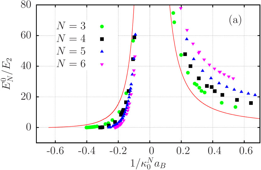
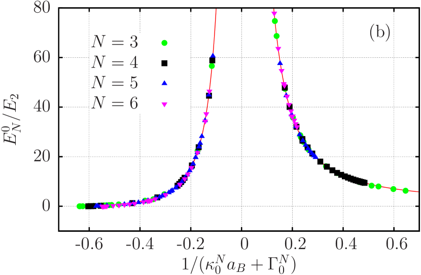
Figure 2: (color online). The ground-state N-body binding-energy $E^{0}_{N}$ in units of $E_{2}$ as a function of (a) $1/\kappa_{0}^{N}a_{B}$, and (b) $1/(\kappa_{0}^{N}a_{B}+\Gamma_{0}^{N}$). $E_{2}$ is the two-body binding energy for $a>0$, and the two-body virtual state energy for $a<0$. In panel (b) the ground-state energies in terms of the scaled variable collapse onto the zero-range curve (solid line).

In Fig. 2(a) we show selected results for the $N=3,4,5,6$ ground-state binding energies. The $N$-body ground-state binding energies $E_{N}^{0}$ are divided by $E_{2}$, which is the two-body binding energy for $a>0$ or the virtual-state energy for $a<0$. These ratios are given as a function of the inverse of the control parameter $\kappa_{0}^{N}a_{B}$. The parameter $\kappa_{0}^{N}$ is fixed by the $N$-body ground-state binding energy $E_{N}^{0}=\hbar^{2}(\kappa_{0}^{N})^{2}/m$ calculated at the unitary limit $1/a=0$. The corresponding values and some relevant ratios are given in Table 1. The solid curve represents the result of the $N=3$ zero-range theory given in Eq. (1) for $n=n^{*}$. The results for the different clusters have been obtained using both TBG and PT potentials. In the figure only a subset of the numerical data is shown in order to better appreciate the trend.

In Fig. 2(b) the same data are shown, but this time the control parameter, $\kappa_{0}^{N}a_{B}$, has been shifted by a quantity $\Gamma^{N}_{0}$, different for each particle sector. As a remarkable result, the different sets of data collapse on the three-body zero-range universal curve. This is very reminiscent of the scaling property in critical phenomena Stanley (1999). In our case we have a $N$-dependent parameter, $\kappa_{0}^{N}$, that fixes the scale of the system and, in this respect, we refer here to it as a scaling parameter. Furthermore an $N$-dependent parameter, $\Gamma_{0}^{N}$ appears to take into account finite-range corrections. In this respect we refer to it as a finite-range scaling parameter.

It should be noticed that the values of $\kappa_{0}^{N}$ has been obtained from our data, and in doing so we have included some range corrections into these quantities. As it is well known, the lower energy states, as those considered here, have some dependence on the form of the potential. This dependence decreases in higher level states Deltuva (2013). However, we want to emphasize that $\kappa_{0}^{N}$ are not new $N$-body parameters in the same sense as the emergent three-body parameter $\kappa_{*}$. In the present treatment, where we only use two-body interaction (eventually, we could have also added three-body interactions Gattobigio et al. (2012)), there are not such a thing as four-, five-, and six-body parameters; in the scaling limit all their values are fixed by the three-body parameter $\kappa_{*}$, as discussed below (for a different point of view see Ref. Hadizadeh et al. (2011)).

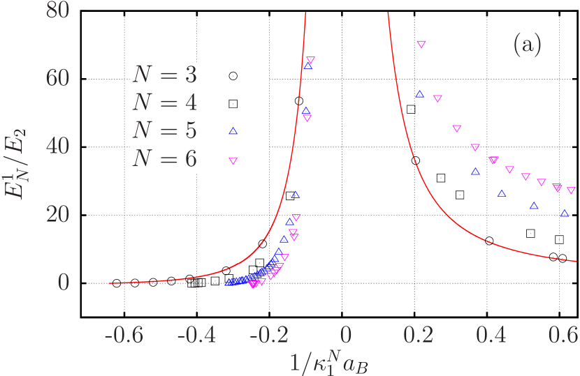
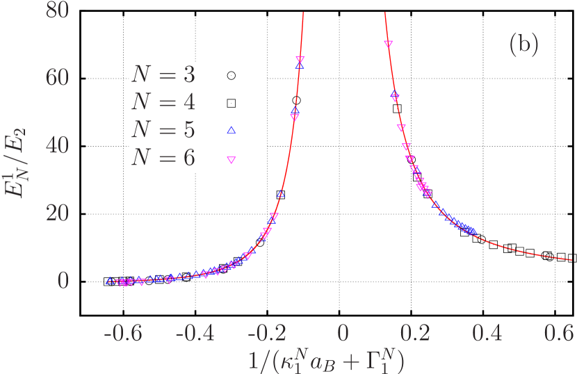
Figure 3: (color online). The excited-state N-body binding-energy $E^{1}_{N}$ in units of $E_{2}$ as a function of (a) $1/\kappa_{1}^{N}a_{B}$, and (b) $1/(\kappa_{1}^{N}a_{B}+\Gamma_{1}^{N}$). $E_{2}$ is the two-body binding energy for $a>0$, and the two-body virtual state for $a<0$. In panel (b) the excited-state energies in terms of the scaled variable collapse onto the zero-range curve (solid line).

In Fig. 3(a) we show our calculations for the $N$-body excited states $E^{1}_{N}$. We report the ratios $E_{N}^{1}/E_{2}$, where $E_{2}$ is still either the two-body binding energy for $a>0$ or the virtual-state energy for $a<0$, as a function of the inverse of the control parameter $\kappa_{1}^{N}a_{B}$. As for the ground states, the parameters $\kappa_{1}^{N}$ are fixed by the excited-binding energy $E^{1}_{N}=\hbar^{2}(\kappa_{1}^{N})^{2}/m$ at the unitary limit. The solid line shows the universal function. Again, we want to stress that they are not new $N$-body parameters, but they are fixed by the value of $\kappa_{*}$. As before, $\kappa_{1}^{N}$ has some range corrections which can be estimated in the case of $N=3$ from Table 1. The zero-range theory imposes $\kappa_{0}^{3}/\kappa_{1}^{3}\approx 22.7$ whereas we found $\approx 23.0$ and $\approx 22.4$ using TBG and PT potentials respectively.

In Fig. 3(b) our data sets are shown with a shift in the control variable $\kappa_{1}^{N}a_{B}$ by a $N$-dependent quantity $\Gamma_{1}^{N}$. As for the ground states, the excited states collapse on the universal curve too, pointing out to the emergence of a common universal behaviour in the $N$-boson system.

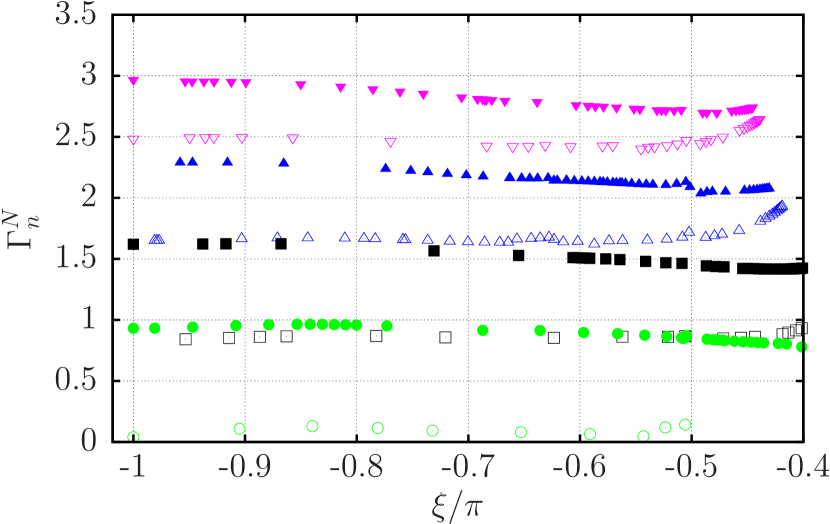
Figure 4: The finite-range scaling parameters $\Gamma_{n}^{N}$ as a function of the angle $\xi$ derived from Eq. (5). The symbols are the same as in Figs. 2 and 3.

Our numerical findings can be summarized in a modified version of Eq. (1). We propose

$$\begin{gathered}E_{N}^{n}/E_{2}=\tan^{2}\xi\\ \kappa_{n}^{N}a_{B}+\Gamma_{n}^{N}=\frac{\text{e}^{-\Delta(\xi)/2s_{0}}}{\cos\xi}\,.\end{gathered}$$ (5)

where the function $\Delta(\xi)$ is universal and it is determined by the three-body physics. The above equation, valid for general $N$, shows the same universal character of the three-boson system and, due to the DSI, with the same universal function $\Delta(\xi)$. The parameter $\kappa_{n}^{N}$ appears as a scale parameter and the shift $\Gamma_{n}^{N}$ is a finite-range scale parameter introduced to take into account finite-range corrections. The introduction of the shifts $\Gamma_{n}^{N}$ is probably a first-order correction of finite-range effects. In fact, we can use Eq. (5) to see that a small dependence on the parameter $\xi$ still remains. This is illustrated in Fig. 4 in which $\Gamma_{n}^{N}$ is obtained by subtracting to the universal term $\text{e}^{-\Delta(\xi)/2s_{0}}/{\cos\xi}$ the computed value $\kappa_{n}^{N}a_{B}$ at the corresponding values of the angle $\xi$.

Finally, we want to comment on the scaling parameters $\kappa_{n}^{N}$. In the zero-range limit, their values are fixed by the three-body parameter $\kappa_{*}$. For instance, in $N=3$ we have defined $\kappa^{3}_{n}=\text{e}^{-(n-n^{*})\pi/s_{0}}\kappa_{*}$, and in the four-body sector an accurate study gives $\kappa^{4}_{0}=2.147\kappa_{0}^{3}$ Deltuva (2013). In Table 1 we report our values for TBG potential , and when available, the zero-range-limit values. From the table we can deduce a linear relation between the ground states that can be approximated as

$$\frac{\kappa_{0}^{N}}{\kappa_{0}^{3}}=1+(N-3)(\frac{\kappa_{0}^{4}}{\kappa_{0}^{3}}-1)\,.$$ (6)

In the scaling limit, using the universal value of $\kappa_{0}^{4}/\kappa_{0}^{3}$, this relation reduces to $\kappa_{0}^{N}/\kappa_{0}^{3}=1+1.147(N-3)$. The linear relation with $N$ can also been seen in Refs. von Stecher (2010); Hanna and Blume (2006).

	$N=3$	$N=4$	$N=5$	$N=6$
$\kappa_{0}^{N}r_{0}$	$4.88\cdot 10^{-1}$	$1.18$	$1.96$	$2.77$
$\kappa_{1}^{N}r_{0}$	$2.12\cdot 10^{-2}$	$5.11\cdot 10^{-1}$	$1.24$	$2.07$
$\kappa_{0}^{N}/\kappa_{1}^{N}$	23.0 (22.7Efimov (1970))	2.31	1.58	1.34
$\kappa_{0}^{N}/\kappa_{0}^{N-1}$	-	2.42 (2.147Deltuva (2013))	1.66	1.41
$\kappa_{1}^{N}/\kappa_{0}^{N-1}$	-	1.05 (1.001Deltuva (2013))	1.05	1.06
$\kappa_{1}^{N}/\kappa_{1}^{N-1}$	-	24.1	2.43	1.67

Table 1: We report the parameters $\kappa_{n}^{N}$, in unit of $r_{0}$, and selected ratios for the TBG potential. When available, we report the ratios at the scaling limit between parenthesis.

To summarize, we have extended to the $N$-boson systems the concept of universality inside the Efimov window. By introducing $N$-body scaling parameters $\kappa_{n}^{N}$ and finite-range corrections, $\Gamma_{n}^{N}$ and $a_{B}$, we have demonstrated that scaled ground- and excited-state energies of systems up to (at least) $N=6$ collapse over the same universal curve, described by the universal function appearing in Eq.(5) (for the ensemble of all the calculated data see the Supplemental material Note (1)).

As an application, we have shown that our finite-range analysis reconciles experimental measurements of trimer-binding energies on $\ {}^{7}$Li Machtey et al. (2012) with the universal theory, showing the collapse of the data on the universal curve.

I Supplemental material

I.1 Calculation with Pöschl-Teller potential

The Pöschl-Teller (PT) potential has the following form

$$V_{\epsilon}(r)=-\frac{\hbar^{2}}{mb^{2}}\,\frac{2(1+C\epsilon)}{\epsilon^{2}\cosh^{2}(r/b\epsilon)}\,,$$ (S1)

where $b$ is a length scale, $m$ the mass of the identical particles, and $C$ and $\epsilon$ are numbers. The potential is a local-potential representation of the contact interaction in the limit $\epsilon\rightarrow 0$ Kruppa et al. (2001).

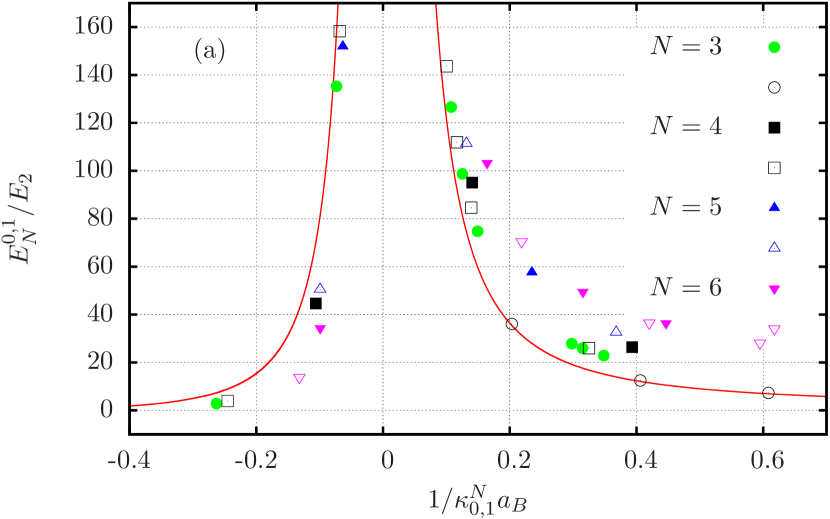
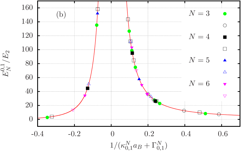
Figure S1: The ground- and excited-state N-body binding energies $E_{N}^{0,1}$ of Pösch-Teller potential, Eq. (S1), in units of $E_{2}$ as a function of (a) $1/\kappa_{0,1}^{N}a_{B}$, and (b) $1/(\kappa_{0,1}^{N}a_{B}+\Gamma_{0,1}^{N}$). $E_{2}$ is the two-body binding energy for $a>0$, and the two-body virtual state energy for $a<0$. In panel (b) the ground- and excited-state energies in terms of the scaled variable collapse onto the zero-range curve (solid line).

We made our calculations setting $\epsilon=1$ and varying $C$ in order to change the scattering length. We calculated both ground- and excited-state energies for $N=3,4,5,6$, and a selection of our results are shown in Fig. S1; on Fig. S1(a) we present our calculation without shift, while data in Fig. S1(b) are shifted and we see that they collapse over the universal curve. Moreover, in Table S1 we report a summary of the shifts and the energies at the unitary limit for PT potential.

	$N=3$	$N=4$	$N=5$	$N=6$
$\kappa_{0}^{N}b$	0.3668	0.9088	1.521	2.175
$\kappa_{1}^{N}b$		0.3934	0.971	1.633
$\kappa_{0}^{N}/\kappa_{1}^{N}$		2.31	1.58	1.33
$\kappa_{0}^{N}/\kappa_{0}^{N-1}$	-	2.48	1.68	1.43
$\kappa_{1}^{N}/\kappa_{0}^{N-1}$	-	1.07	1.07	1.07
$\kappa_{1}^{N}/\kappa_{1}^{N-1}$	-		2.46	1.68
$\Gamma_{0}^{N}$	0.93	1.63	2.34	3.10
$\Gamma_{1}^{N}$	-	0.98	1.92	2.77

Table S1: We report the parameters $\kappa_{n}^{N}$, in unit of $b$, $\Gamma_{n}^{N}$, and selected ratios for the Pöschl-Teller potential.

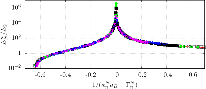
Figure S2: (color online). Ground- and excited-state N-body binding-energies $E^{n}_{N}$ in units of $E_{2}$ as a function of $1/(\kappa_{n}^{N}a_{B}+\Gamma_{n}^{N})$. $E_{2}$ is the two-body binding energy for $a>0$, and the two-body virtual state for $a<0$. The symbols are the same as in Fig. 2 and Fig. 3 of the paper. All the data collapse on the three-body universal curve (solid line) calculated in the scaling limit.

In Fig. S2 we report all the calculated data, both with Gaussian and PT potential.

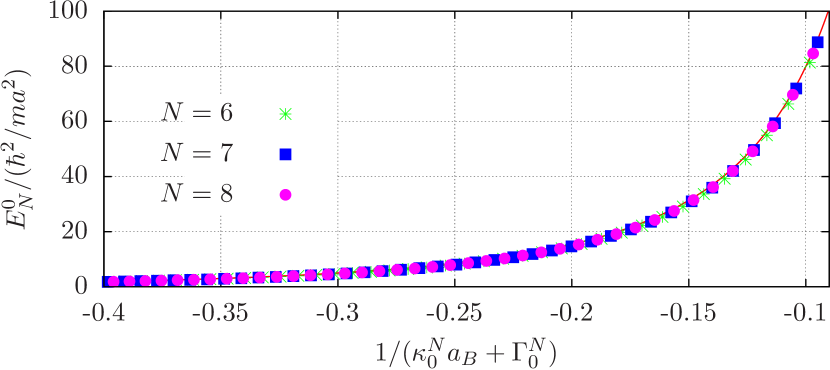
Figure S3: The ground-state N-body binding-energy $E^{0}_{N}$ from Ref. von Stecher (2010) in units of $\hbar^{2}/ma^{2}$ as a function of $1/(\kappa_{0}^{N}a+\Gamma_{0}^{N})$. The solid curve represent the universal zero-range curve.

I.2 Analysis of published calculations of [J. von Stecher, J. Phys. B: At. Mol. Opt. Phys. 43, 101002 (2010)].

We have applied Eq.(5) of our paper to analyse the calculation of Ref. von Stecher (2010). In that paper the author performed few-body calculations using two- plus three-body Gaussian potentials for $N=6$, and a two-body square-well potential plus three-body hard-wall potential for $N=7,8$. In that paper the author gives a four-parameter parametrization of the ground-state energies for $N=6,7,8$, and we have used that parametrization in order to reconstruct the calculated data.

	$N=6$	$N=7$	$N=8$
$\kappa_{0}^{N}/\kappa_{0}^{3}$	4.29	5.22	6.18
$\Gamma_{0}^{N}$	-0.393	-0.414	-0.382

Table S2: We report the parameters $\kappa_{0}^{N}$, in unit of $\kappa_{0}^{3}$, and $\Gamma_{n}^{N}$, used to analysis data of Ref. von Stecher (2010).

In Fig. S3 we show that the extracted data, once analysed with Eq.(5) of our paper, collapse onto the universal zero-range curve. As a side effect, we see that only two-parameters are needed to describe data, and that the collapse does not depend on the Gaussian form of the potential. In Table S2 we report the parameters we used to collapse the data.