A New Sensitivity Analysis and Solution Method for Scintillometer Measurements of Area-Averaged Turbulent Fluxes

Abstract

Scintillometer measurements of the turbulence inner-scale length $l_{o}$ and refractive index structure function $C_{n}^{2}$ allow for the retrieval of large-scale area-averaged turbulent fluxes in the atmospheric surface layer. This retrieval involves the solution of the non-linear set of equations defined by the Monin-Obukhov similarity hypothesis. A new method that uses an analytic solution to the set of equations is presented, which leads to a stable and efficient numerical method of computation that has the potential of eliminating computational error. Mathematical expressions are derived that map out the sensitivity of the turbulent flux measurements to uncertainties in source measurements such as $l_{o}$. These sensitivity functions differ from results in the previous literature; the reasons for the differences are explored.

guessConjecture

Appl. Opt. 903 Koyukuk Dr. 99775, Fairbanks, AK. Ph: 1-907-474-7602 Fx: 1-907-474-7290

“Iteration, like friction, is likely to generate heat instead of progress.” - George Eliot

1 Introduction

Scintillometers detect fluctuations in the intensity of a beam of light that passes through a path length of 50 m to 5000 m of near-ground turbulence in the surface layer [Kleissl et al. (2008)]. These fluctuations are related to the structure function of the index of refraction $C_{n}^{2}$, and the turbulence inner-scale length $l_{o}$ [Tatarski (1961), Hill (1988), Sasiela (1994)]. The index of refraction is a function of temperature and humidity; thus $C_{n}^{2}$ can be decomposed into structure functions of temperature $T$ and humidity $q$ as $C_{T}^{2}$, $C_{Tq}$ and $C_{q}^{2}$. Scintillometer wavelengths are selected that are each more sensitive to fluctuations in one variable (such as temperature) than others (such as humidity), so that $C_{T}^{2}$, $C_{Tq}$ and $C_{q}^{2}$ may be resolved. For example, intensity fluctuations of visible and near-infrared beams are more sensitive to temperature fluctuations than humidity fluctuations, while microwave beams are more sensitive to humidity fluctuations [Andreas (1990)]. Structure functions such as $C_{n}^{2}$ are described in TATARSKI, and represent the strength and spacial frequency of perturbations in variables; thus $C_{n}^{2}$ is a measure of turbulence intensity weighted by the susceptibility of the index of refraction of the medium to changes in variables such as temperature and humidity.

The goal of this study is to solve for the sensible heat flux $H_{S}$ and the momentum flux $\tau$ as functions of source measurements such as $C_{n}^{2}$ and $l_{o}$, as well as to quantify the propagation of uncertainty from source measurements to the calculated values of $H_{S}$ and $\tau$. Another type of turbulent flux is the latent heat flux $H_{L}$. The turbulent fluxes are given by

$$H_{S} = -\rho c_{p}u_{\star}T_{\star},$$ (1)

$$H_{L} = -L_{v}u_{\star}q_{\star},$$ (2)

$$\tau = \rho{u_{\star}}^{2},$$ (3)

where $T_{\star}$ and $q_{\star}$ are the temperature and humidity scales, $u_{\star}$ is the friction velocity, $\rho$ is the density of the air, $c_{p}$ is the specific heat at constant pressure, and $L_{v}$ is the latent heat of vaporization. Determining area-averaged turbulent fluxes involves solving for $T_{\star}$ and $q_{\star}$, which are related to the path-length scale structure-function measurements through the non-linearly coupled Monin-Obukhov similarity equations [Sorbjan (1989)]. This procedure also involves solving for $u_{\star}$ in Eqs. 1, 2 and 3. The friction velocity $u_{\star}$ can be related either to path-length scale $l_{o}$ measurements as with displaced-beam scintillometer strategies described in ANDREAS1992, or to the wind profile and roughness length with large-aperture scintillometer strategies via the Businger-Dyer relation [Panofsky and Dutton (1984), Sorbjan (1989), Lagouarde et al. (2002), Hartogensis et al. (2003)].

We consider here a displaced-beam scintillometer strategy in which path-averaged measurements of $C_{n}^{2}$ and $l_{o}$ are obtained. Other required measurements include temporally-averaged pressure $p$, temperature $T$, humidity $q$, as well as the height of the beam above the underlying terrain $z$. Thus $C_{n}^{2}$, $l_{o}$, $p$, $T$, $q$ and $z$ are referred to as the source measurements. Each of these measurements demonstrates temporal and spacial variability as well as measurement uncertainty. Uncertainty propagates from the source measurements to the derived variables via the set of equations being considered. Uncertainties in $l_{o}$ and $C_{n}^{2}$ are described in HILL1988L0, while uncertainties in $p$, $T$ and $q$ depend on the particular instrument being used. Here, we explore the use of scintillometers over flat and homogeneous terrain, thus the height of the beam $z$ is considered to be a single value with its associated uncertainty. While $C_{n}^{2}$ and $l_{o}$ are representative of turbulent fluctuations along the whole beam, $p$, $T$ and $q$ are typically point measurements representative of localized areas near their respective instruments.

Applications for scintillometers include agricultural scientific studies such as HOEDJESOLIVES and FOKEN, and aggregation of surface measurements to satellite-retrieval scales for weather prediction and climate monitoring as in BEYRICH2002 and in MARX. The unique spacial scale of scintillometer measurements gives them the potential for a key role in bridging the gap between ground-based instruments with footprints on the order of $100$ $\mbox{m}^{2}$ and model and satellite-retrieval scales on the order of $1$ $\mbox{km}^{2}$.

The scale of scintillometer measurements introduces an additional complexity in the retrieval of the turbulent fluxes. This retrieval combines the large-scale scintillometer measured variables $C_{n}^{2}$ and $l_{o}$ with source measurements that are not necessarily representative of the same scale. The only exception to be considered is the atmospheric pressure $p$. In particular, measurements of $T$ and $q$ may be representative of smaller footprints around their respective instruments. Specifically, assuming that variables such as average temperature T represent the entire beam path introduces a form of uncertainty. This uncertainty is somewhat similar to a systematic error, although it may be difficult to quantify because of its temporal variability.

Of previous scintillometer sensitivity studies, some stand out as possibly contradicting each other. For instance, the conclusion of the error analysis in MORONI for a $l_{o}$ and $C_{n}^{2}$ strategy was that “The Monte Carlo analysis of the propagation of the statistical errors shows that there is only moderate sensitivity of the flux calculations to the initial errors in the measured quantities.” The error analysis of ANDREAS1992, however, results in sensitivity functions that feature singularities. The sensitivity functions presented there imply that the resolution of $u_{\star}$ and consequently of $H_{S}$, $H_{L}$ and $\tau$ by scintillometer $l_{o}$ and $C_{n}^{2}$ measurements is intrinsically restricted to low precision over a certain range of environmental conditions. While these two studies use different methods and present results over slightly different ranges in variables, they produce sensitivity functions that for the same range differ significantly.

In Sect. 2 below, we decouple the set of equations including those of the Monin-Obukhov similarity hypothesis for $l_{o}$ and $C_{n}^{2}$ scintillometer strategies for the example of unstable surface-layer conditions to arrive at single equations in single unknowns. The variable inter-dependency is mapped out as illustrated by tree diagrams. In Sect. 3, we take advantage of the mapped out variable inter-dependency to guide us in using the chain rule to solve the global partial derivatives in sensitivity functions to investigate error propagation. We produce sensitivity functions for $H_{S}$, $\tau$ and $u_{\star}$ as functions of both $l_{o}$ and $z$. In Sect. 4 we explore the ramifications of our results and compare them to previous literature, and we give conclusions in Sect. 5.

2 Measurement Strategy Case Study: Displaced-Beam Scintillometer System in Unstable Conditions

We consider here a two-wavelength system as introduced in ANDREAS1989, where one of the scintillometers measures both $l_{o}$ and $C_{n}^{2}$ as in ANDREAS1992. With this strategy, our measurements can resolve humidity and temperature fluctuations separately since the two scintillometers have different wavelengths $\lambda_{1}$ and $\lambda_{2}$ that have differing sensitivities in the index of refraction to humidity and temperature. This technique therefore requires fewer assumptions than the corresponding single-wavelength strategies as seen in ANDREAS1989.

The following set of equations determines $T_{\star}$, $q_{\star}$ and $u_{\star}$ from the source measurements, and subsequently determines the turbulent fluxes:

$$\rho = \frac{p}{RT},$$ (4)

$$l_{o} = \frac{(9\Gamma(1/3)KD(\rho,T))^{3/4}}{\epsilon^{1/4}},$$ (5)

$$\zeta = \frac{zg\kappa}{{u_{\star}}^{2}T}\left(T_{\star}+\frac{0.61T}{\rho+0.61q}q_{\star}\right),$$ (6)

$${u_{\star}}^{3} = \frac{\kappa z\epsilon}{\phi(\zeta)},$$ (7)

$${C_{n_{1}}^{2}} = z^{-2/3}g(\zeta)(A_{1}(\lambda_{1},p,T,q)T_{\star}+B_{1}(\lambda_{1},p,T,q)q_{\star})^{2},$$ (8)

$${C_{n_{2}}^{2}} = z^{-2/3}g(\zeta)(A_{2}(\lambda_{2},p,T,q)T_{\star}+B_{2}(\lambda_{2},p,T,q)q_{\star})^{2},$$ (9)

where $g$ is the local acceleration due to gravity, $\Gamma$ is the Gamma function, $\epsilon$ is the turbulent energy dissipation rate, $R$ is the specific gas constant, $\kappa$ is the von Kármán constant, $\zeta\equiv z/L$, where $L$ is the Obukhov length, $K$ is the Obukhov-Corrsin constant, $\nu(T,\rho)$ is the viscosity of air and $D(T,\rho)$ is the thermal diffusivity of air (Andreas, 1989; 1992; 2012) $C_{n_{1}}^{2}$ and $C_{n_{2}}^{2}$ are structure functions of the refractive index for the separate wavelengths $\lambda_{1}$ and $\lambda_{2}$. Eqs. 4 and 5 determine $\epsilon$ directly from $l_{o}$ and the other source measurements. Inherent in Eqs. 8 and 9 is the assumption that $C_{Tq}=\sqrt{{C_{T}^{2}}{C_{q}^{2}}}$, which is validated previously [Hill (1989), Andreas (1990)].

The similarity functions $g(\zeta)$ and $\phi(\zeta)$ are given by

$$g(\zeta)=a(1-b\zeta)^{-2/3},$$ (10)

$$\phi(\zeta)=(1+d(-\zeta)^{2/3})^{3/2},$$ (11)

for $L<0$ which corresponds to unstable conditions. The form of the similarity functions and their parameters follow from WYNGARD1971 and WYNGARD1971phi; the values are taken to be $a=4.9$, $b=6.1$, and $d=0.46$ [Andreas (1988)].

The source measurements may not determine the sign of $L$, which is unknown a priori for every set of source measurements at any one time interval. We follow ANDREAS1989 in solving for $T_{\star}$ and $q_{\star}$ from Eqs. 8 and 9, making sure to note that the signs of $\left(A_{1,2}T_{\star}+B_{1,2}q_{\star}\right)$ are not yet solved by introducing unknowns $\mbox{sign}_{1}$ and $\mbox{sign}_{2}$:

$$\frac{\mbox{sign}_{1}\sqrt{{C_{n_{1}}^{2}}}z^{1/3}(1-b\zeta)^{1/3}}{\sqrt{a}} = A_{1}T_{\star}\left(1+\frac{B_{1}}{A_{1}}\frac{q_{\star}}{T_{\star}}\right),$$ (12)

$$\frac{\mbox{sign}_{2}\sqrt{{C_{n_{2}}^{2}}}z^{1/3}(1-b\zeta)^{1/3}}{\sqrt{a}} = A_{2}T_{\star}\left(1+\frac{B_{2}}{A_{2}}\frac{q_{\star}}{T_{\star}}\right),$$ (13)

where the roots on the left-hand side are considered to be positive. Following ANDREAS1989, these can be re-arranged to isolate $T_{\star}$ and $q_{\star}$ with the as yet undetermined signs:

$$T_{\star} = \frac{(1-b\zeta)^{1/3}z^{1/3}}{\sqrt{a}}\left(\frac{\mbox{sign}_{1}\sqrt{{C_{n_{1}}^{2}}}B_{2}-\mbox{sign}_{2}\sqrt{{C_{n_{2}}^{2}}}B_{1}}{A_{1}B_{2}-A_{2}B_{1}}\right),$$ (14)

$$q_{\star} = \frac{(1-b\zeta)^{1/3}z^{1/3}}{\sqrt{a}}\left(\frac{\mbox{sign}_{2}\sqrt{C_{n_{2}}^{2}}A_{1}-\mbox{sign}_{1}\sqrt{{C_{n_{1}}^{2}}}A_{2}}{A_{1}B_{2}-A_{2}B_{1}}\right),$$ (15)

where

$$\mbox{sign}_{1,2}=\mbox{sign}[A_{1,2}T_{\star}(1+\frac{B_{1,2}}{A_{1,2}}\frac{q_{\star}}{T_{\star}})].$$ (16)

It is useful to include the definition of the Bowen ratio as

$$\beta\equiv H_{S}/H_{L}=\frac{\rho c_{p}}{L_{v}}\frac{T_{\star}}{q_{\star}}.$$ (17)

We can solve for $\beta$ as

$$\beta=E\left(\frac{\mbox{sign}_{1}\sqrt{C_{n_{1}}^{2}}B_{2}-\mbox{sign}_{2}\sqrt{{C_{n_{2}}^{2}}}B_{1}}{\mbox{sign}_{2}\sqrt{C_{n_{2}}^{2}}A_{1}-\mbox{sign}_{1}\sqrt{C_{n_{1}}^{2}}A_{2}}\right),$$ (18)

where $E(T,p)=\rho c_{p}/L_{v}$. It is useful to consider $\beta$ as well as $\zeta$ as unit-less independent variables in our sensitivity analyses that represent certain meteorological regimes. They represent the ratio of the sensible to latent heat fluxes and an indicator of surface-layer stability, respectively.

Since we are considering unstable conditions, we have $\zeta<0$ since $L<0$, so from Eq. 6 we have

$$T_{\star}(1+\frac{0.61T}{\rho+0.61q}\frac{q_{\star}}{T_{\star}})<0,$$ (19)

$$(1-b\zeta)>0,$$ (20)

$$(1+d(-\zeta)^{2/3})^{3/2}>0,$$ (21)

We begin decoupling the set of equations by taking Eqs. 14 and 15 and substituting into Eq. 6, then cubing the resulting equation as well as squaring Eq. 7 to arrive at

$$\zeta^{3} = \frac{z^{4}g^{3}\kappa^{3}(1-b\zeta)}{{u_{\star}}^{6}T^{3}a^{3/2}}\left[F^{3}(1+H/\beta)^{3}\right],$$ (22)

$${u_{\star}}^{6} = \frac{\kappa^{2}z^{2}\epsilon^{2}}{(1+d(-\zeta)^{2/3})^{3}},$$ (23)

where $F(T,p,q,\lambda_{1},\lambda_{2},C_{n_{1}}^{2},C_{n_{2}}^{2})$ and $H(T,p,q)$ are defined as

$$F(T,p,q,\lambda_{1},\lambda_{2},C_{n_{1}}^{2},C_{n_{2}}^{2}) = \frac{\mbox{sign}_{1}\sqrt{{C_{n_{1}}^{2}}}B_{2}-\mbox{sign}_{2}\sqrt{{C_{n_{2}}^{2}}}B_{1}}{A_{1}B_{2}-A_{2}B_{1}},$$ (24)

$$H(T,p,q) = E\left(\frac{0.61T}{\rho+0.61q}\right).$$ (25)

We then combine Eqs. 22 and 23 to obtain a final equation in $\zeta$:

$$\zeta^{3}=M(1-b\zeta)(1+d(-\zeta)^{2/3})^{3},$$ (26)

where

$$M\equiv\frac{g^{3}z^{2}\kappa[F^{3}(1+H/\beta)^{3}]}{T^{3}\epsilon^{2}a^{3/2}},$$ (27)

is determined directly from the source measurements. Here we note that the left-hand side is negative, and so the term in square brackets in $M$ is negative as well. From any set of measurements we know the sign of $A_{1}B_{2}-A_{2}B_{1}$, and we also know the values of the two terms that multiply the unknown signs. Occasionally these relations are enough to determine all the signs; otherwise the signs remain ambiguous and they are evaluated from observations of the temperature and humidity stratification as seen in ANDREAS1989.

Eq. 26 can be solved with a fixed-point recursive technique as illustrated in Fig. 1. The recursive function

$$\zeta=V(\zeta)\equiv M^{1/3}(1-b\zeta)^{1/3}(1+d(-\zeta)^{2/3})$$ (28)

is used.

Figure 1: Visualization of the solution of Eq. 26 using fixed-point recursion, with $M=-1/3$. The function $\zeta=V(\zeta)$ is used, where
$V(\zeta)\equiv M^{1/3}(1-b\zeta)^{1/3}(1+d(-\zeta)^{2/3})$. Real roots of $M^{1/3}$ are chosen. The recursive series $[V(\zeta_{guess}),V(V(\zeta_{guess})),V(V(V(\zeta_{guess}))),V(V(V(V(\zeta_{guess}))))...]$ converges for any $\zeta_{guess}<0$.

A solution of Eq. 26 using fixed-point recursion is seen in Fig. 2.

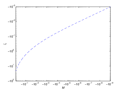
Figure 2: Solution of Eq. 26 using fixed-point recursion on the function $\zeta=V(\zeta)$ where $V(\zeta)\equiv M^{1/3}(1-b\zeta)^{1/3}(1+d(-\zeta)^{2/3})$. Real roots of $M^{1/3}$ are chosen. Note that for $M=-1/3$, we have $\zeta\approx-5.5$ as in Fig. 1. Computational error was verified to be completely negligible with minimal running time involved.

A good estimate of the uncertainty in the derived variables that results from small errors in source measurements is given by

$${\sigma_{f}}=\sum_{i=1}^{N}\left({\frac{\partial f}{\partial x_{i}}}\right)\sigma_{x_{s_{i}}}+\sqrt{\sum_{i=1}^{N}\left({\frac{\partial f}{\partial x_{i}}}\right)^{2}{\sigma^{2}}_{x_{r_{i}}}}+\sigma_{f_{c}},$$ (29)

where the derived variable $f$ is a function of source measurement variables $x_{1},x_{2},...,x_{N}$ with respective systematic error $\sigma_{x_{s_{1}}},\sigma_{x_{s_{2}}},...,\sigma_{x_{s_{N}}}$ and with respective independent Gaussian distributed uncertainties with standard deviations $\sigma_{x_{r_{1}}},\sigma_{x_{r_{2}}},...,\sigma_{x_{r_{N}}}$ as seen in TAYLOR. The numerical indices indicate different independent variables, such as $T$, $p$, or $z$, for example. Computational error $f$ due to the inaccurate solution of the theoretical equations is represented by $\sigma_{f_{c}}$. The first and last terms in Eq. 29 represent an offset from the true solution (inaccuracy), whereas the central square-root term represents the breadth of uncertainty due to random error (imprecision).

It is practical for the purpose of a sensitivity study to rewrite Eq. 29 as

$$\frac{\sigma_{f}}{f}=\sum_{i=1}^{N}S_{f,x}\frac{\sigma_{x_{s_{i}}}}{x_{s_{i}}}+\sqrt{\sum_{i=1}^{N}S_{f,x}^{2}\frac{{\sigma^{2}}_{x_{r_{i}}}}{{x_{r_{i}}}^{2}}}+\frac{\sigma_{f_{c}}}{f},$$ (30)

where $S_{f,x}$ are unitless sensitivity functions defined by

$$S_{f,x}\equiv\frac{x}{f}\left(\frac{\partial f}{\partial x}\right).$$ (31)

The sensitivity functions are each a measure of the portion of the error in the derived variable $f$ resulting from error on each individual source measurement $x$. In addition to the error on source measurement variables, we can also recognize that $a$, $b$ and $d$ have been resolved to some level of certainty by fitting field data. We thus treat them here in the same way as source measurements.

In the application of Eqs. 29 and 30, we recognize the addition of the computational error $\sigma_{f_{c}}$. In previous field and sensitivity studies [Lagouarde et al. (2002), deBruin et al. (2002), Solignac et al. (2009), Andreas (2012)], the full set of equations has been incorporated into a cyclically iterative algorithm which cycles through the full set of equations, allowing multiple variables to change. This numerical algorithm sometimes fails to converge, as demonstrated in ANDREAS2012.

The problem of resolving the uncertainty on the derived variables is a matter of identifying the magnitude and character of the source measurement uncertainties, and then solving for the partial derivative terms in Eqs. 29 and 31. These derivatives are global ; that is, they take into account all the relationships in all of the relevant equations through which the variable $f$ is derived. Without an analytic solution of the set of coupled equations we could either solve for the partial derivatives through a total-differential expansion of each equation individually, followed by a re-grouping of all differential terms as seen in Andreas (1989; 1992) or we could use numerical error propagation techniques as in the Monte Carlo analysis of MORONI or as in the analysis of SOLIGNAC.

We investigate inter-variable sensitivity analytically via Eq. 31, using Eq. 26 as a starting point. We use Eq. 26 to determine the details of the variable inter-dependency to define our use of the chain rule. A tree diagram representing the variable inter-dependency is broken into three parts shown in Figs. 3, 4, and 5.

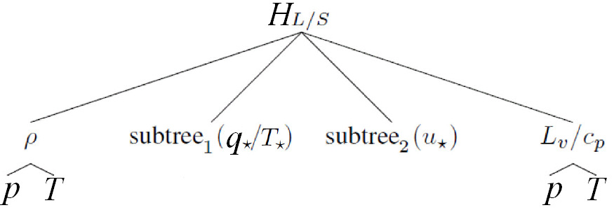
Figure 3: Variable inter-dependency tree diagram for a two-wavelength measurement strategy inferring $H_{L/S}$ through path-averaged $u_{\star}$ and $q_{\star}/T_{\star}$ measurements via scintillometer measurements of $l_{o}$ and $C_{n}^{2}$ under unstable meteorological conditions ($\zeta<0$). Variables at the bottom of the tree are source measurements; all others are considered to be derived variables. The “$/$” symbol is meant to delineate between two independent tree diagrams. Note that $H_{L}$ is not a direct function of $\rho$; this branch is for the convenience of including $H_{S}$ since the rest of their tree diagrams are identical. Figs. 4 and 5 feature $\mbox{subtree}_{1}$ and $\mbox{subtree}_{2}$, respectively.

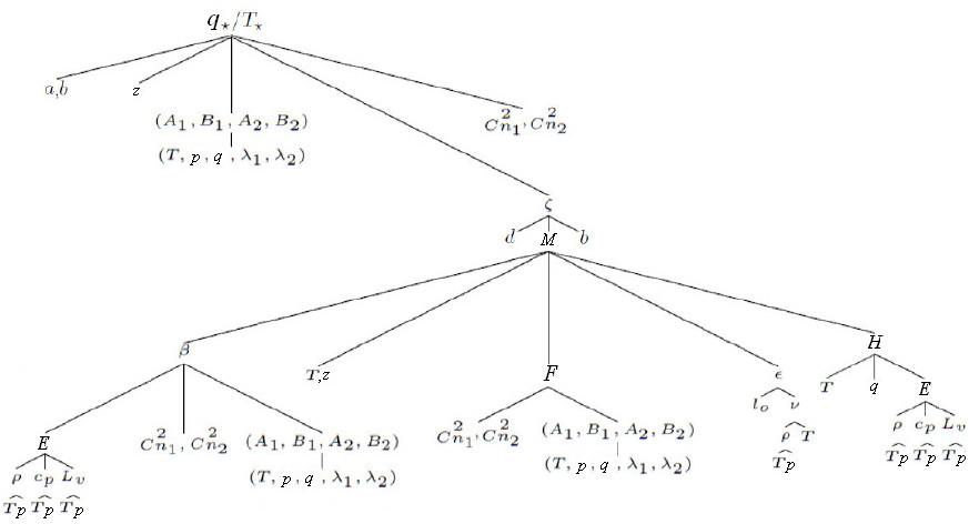
Figure 4: $\mbox{Subtree}_{1}$ of variable inter-dependency for $\zeta<0$. The main tree diagram is seen in Fig. 3.

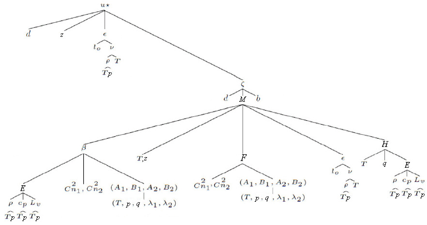
Figure 5: $\mbox{Subtree}_{2}$ of variable inter-dependency for $\zeta<0$. The main tree diagram is seen in Fig. 3.

Eq. 26 can be reduced to a choice of two algebraic equations

$$\alpha>0,-\alpha^{9}=M(1+d\alpha^{2})^{3}(1+b\alpha^{3}),\zeta=-\alpha^{3},\frac{\partial\zeta}{\partial\alpha}=-3\alpha^{2}<0,$$

(32)

$$\alpha<0,\alpha^{9}=M(1+d\alpha^{2})^{3}(1-b\alpha^{3}),\zeta=\alpha^{3},\frac{\partial\zeta}{\partial\alpha}=3\alpha^{2}>0,$$ (33)

with the substitution

$$\alpha^{2}\equiv(-\zeta)^{2/3}>0.$$ (34)

Galois theory implies that, since Eqs. 32 and 33 are ninth order, there is no way to write $\zeta=f(p,T,q,C_{n_{1}}^{2},C_{n_{2}}^{2},\lambda_{1},\lambda_{2},z,l_{o})$ for any general values of $b$ and $d$, where $f$ is an explicit function of the source measurements [Edwards (1984)]. It is thus simplest to extract $\left(\frac{\partial\zeta}{\partial M}\right)$ by implicit differentiation of Eq. 26; the results are in given in Appendix A.

3 Results: Derivation of Sensitivity Functions

Following the solution method described above, we solve for global partial derivative terms in Eqs. 29 and 31 through use of the general chain rule guided by the variable inter-dependency tree diagrams seen in Figs. 3, 4 and 5. We will obtain sensitivity functions of the sensible heat flux $H_{S}$ and the momentum flux $\tau$ as functions of $z$ and $\epsilon$. From Eqs. 1, 5 and 31 we have

$$S_{H_{S},\epsilon} = S_{T_{\star},\epsilon}+S_{u_{\star},\epsilon}=-\frac{1}{4}S_{H_{S},l_{o}},$$ (35)

$$S_{H_{S},z} = S_{T_{\star},z}+S_{u_{\star},z},$$ (36)

and from Eqs. 3, 5 and 31, we have

$$S_{\tau,\epsilon} = 2S_{u_{\star},\epsilon}=-\frac{1}{4}S_{\tau,l_{o}},$$ (37)

$$S_{\tau,z} = 2S_{u_{\star},z},$$ (38)

thus we seek solutions for $S_{T_{\star},z}$, $S_{u_{\star},z}$, $S_{T_{\star},\epsilon}$, and $S_{u_{\star},\epsilon}$.

We first obtain $S_{T_{\star},\epsilon}$ with guidance from the tree diagram depicted in Fig. 4:

$$S_{T_{\star},\epsilon}=\frac{\epsilon}{T_{\star}}\left(\frac{\partial T_{\star}}{\partial\zeta}\right)\left(\frac{\partial\zeta}{\partial M}\right)\left(\frac{\partial M}{\partial\epsilon}\right).$$ (39)

The individual terms of Eq. 39 are given in Appendices A and B. Combining them, we obtain

$$S_{T_{\star},\epsilon}=\frac{1}{3}\left(\frac{2b\zeta(-\zeta)^{1/3}(1+d(-\zeta)^{2/3})}{(3-2b\zeta)(1+d(-\zeta)^{2/3})(-\zeta)^{1/3}+2d\zeta(1-b\zeta)}\right).$$ (40)

We now obtain $S_{T_{\star},z}$:

$$S_{T_{\star},z}=\frac{z}{T_{\star}}\left[\left(\frac{\partial T_{\star}}{\partial z}\right)_{\zeta}+\left(\frac{\partial T_{\star}}{\partial\zeta}\right)_{z}\left(\frac{\partial\zeta}{\partial M}\right)\left(\frac{\partial M}{\partial z}\right)\right].$$ (41)

The individual terms of Eq. 41 are developed in Appendices A and C. Combining them, we obtain

$$S_{T_{\star},z}=\frac{1}{3}\left[1-\left(\frac{2b\zeta(-\zeta)^{1/3}(1+d(-\zeta)^{2/3})}{(3-2b\zeta)(1+d(-\zeta)^{2/3})(-\zeta)^{1/3}+2d\zeta(1-b\zeta)}\right)\right].$$ (42)

We now obtain $S_{u_{\star},\epsilon}$ with guidance from the tree diagram depicted in Fig. 5. We have

$$S_{u_{\star},\epsilon}=\frac{\epsilon}{u_{\star}}\left[\left(\frac{\partial u_{\star}}{\partial\epsilon}\right)_{\zeta}+\left(\frac{\partial u_{\star}}{\partial\zeta}\right)_{\epsilon}\left(\frac{\partial\zeta}{\partial M}\right)\left(\frac{\partial M}{\partial\epsilon}\right)\right].$$ (43)

The individual terms in Eq. 43 are developed in Appendices A and D. Combining them, we obtain

$$S_{u_{\star},\epsilon}=\frac{1}{3}\left[1-\left(\frac{2d\zeta(1-b\zeta)}{(3-2b\zeta)(1+d(-\zeta)^{2/3})(-\zeta)^{1/3}+2d\zeta(1-b\zeta)}\right)\right].$$ (44)

We now obtain $S_{u_{\star},z}$. We have

$$S_{u_{\star},z}=\frac{z}{u_{\star}}\left[\left(\frac{\partial u_{\star}}{\partial z}\right)_{\zeta}+\left(\frac{\partial u_{\star}}{\partial\zeta}\right)_{z}\left(\frac{\partial\zeta}{\partial M}\right)\left(\frac{\partial M}{\partial z}\right)\right].$$ (45)

The individual terms in Eq. 45 are developed in Appendices A and E. Combining them we obtain

$$S_{u_{\star},z}=\frac{1}{3}\left[1+\left(\frac{2d\zeta(1-b\zeta)}{(3-2b\zeta)(1+d(-\zeta)^{2/3})(-\zeta)^{1/3}+2d\zeta(1-b\zeta)}\right)\right].$$ (46)

Combining our results in Eqs. 39, 41, 43, and 45, we can obtain $S_{H_{S},\epsilon}$ and $S_{H_{S},z}$ from Eqs. 35 and 36; the results are seen in Fig. 6.

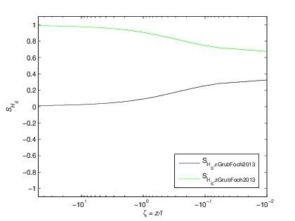
Figure 6: Sensitivity functions for $H_{S}$ with regards to measurements of $\epsilon$ and $z$ in the path-averaged $u_{\star}$ scintillation measurement, for unstable conditions corresponding to $\zeta<0$.

The absolute value of our results for $S_{H_{S},l_{o}}$ given by Eqs. 35, 40 and 44 is similar to the sensitivity multiplier found in MORONI as seen in their Fig. 10. The absolute value of our result of $S_{\tau,l_{o}}$ given by Eqs. 37 and 44 is also compatible with the results of MORONI seen in their Fig. 9. However, our result for $S_{u_{\star},\epsilon}$ in Eq. 44 differs from that obtained in ANDREAS1992 as seen in Fig. 7.

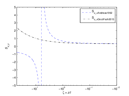
Figure 7: Sensitivity function for $u_{\star}$ with regards to measurements of $\epsilon$ in the path-averaged $u_{\star}$ scintillation measurement. Results from ANDREAS1992 are plotted (denoted there as $S_{\epsilon}$) along with Eq. 44 derived here for $\zeta<0$.

Similarly, our result for $S_{u_{\star},z}$ in Eq. 46 differs from that obtained in ANDREAS1992 as seen in Fig. 8.

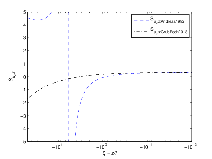
Figure 8: Sensitivity function for $u_{\star}$ with regards to measurements of $z$ in the path-averaged $u_{\star}$ scintillation measurement. Results from ANDREAS1992 are plotted (denoted there as $S_{zz}$) along with Eq. 46 derived here for $\zeta<0$.

4 Discussion

The reason for the difference between our results and those of ANDREAS1992 in Figs. 7 and 8 can be seen to have arisen in Eqs. A.7 and A.10 of ANDREAS1992 . Even though there is a typographical error in Eq. A.7 in the application of the product rule (it should be

$$\frac{\partial\epsilon}{\partial u_{\star}}=\frac{3{u_{\star}}^{2}}{\kappa z}\phi_{\epsilon}(\zeta)+\frac{{u_{\star}}^{3}}{z\kappa}\frac{\partial\phi_{\epsilon}}{\partial\zeta}\frac{\partial\zeta}{\partial u_{\star}},$$ (47)

where the second term contained $u_{\star}^{2}$ originally), this is not the origin of the reason since the result in Eq. A.8 follows from the modified Eq. A.7. The reason is found to be that Eqs. A.7 and A.8 are not differentiated locally with respect to Eq. 1.3 of ANDREAS1992 as they should be in a total-differential expansion. The local derivative is

$$\frac{\partial\epsilon}{\partial u_{\star}}=\frac{\partial}{\partial u_{\star}}\left(\frac{u_{\star}^{3}}{\kappa z}\phi_{\epsilon}(\zeta)\right)=\frac{3{u_{\star}}^{2}}{\kappa z}\phi_{\epsilon}(\zeta)=\frac{3\epsilon}{u_{\star}},$$ (48)

keeping $\zeta$ constant regardless of the relationship between $\zeta$ and $u_{\star}$. The relationship between $\zeta$ and $u_{\star}$ is taken into account when we re-group the full set of locally expanded equations (which are coupled in $\zeta$ and $u_{\star}$). The second term on the right-hand side of Eq. 47 and Eq. A.7 of ANDREAS1992 is thus not necessary and does not appear in Eq. 48. Taking into account the relationship between $\zeta$ and $u_{\star}$ via the chain rule is appropriate for direct evaluation of global derivatives, but not in individual derivatives of a total-differential expansion of the full set of equations. Eqs. A.10 and A.11 of ANDREAS1992 have the same issues of not being differentiated locally with respect to Eq. 1.3 of ANDREAS1992. The local derivative there is

$$\frac{\partial\epsilon}{\partial z}=-\frac{\epsilon}{z}.$$ (49)

A re-analysis of the ANDREAS1992 differential expansion including the local derivatives in Eqs. 48 and 49 is reproduced in Appendix F; the results for $S_{u_{\star},\epsilon}$ and $S_{u_{\star},z}$ are identical to those found here in Eqs. 43 and 45. Note that the left-hand side of Eq. 89 contains the terms $(S_{u_{\star}}-2)$ and $(S_{z}+1)$ instead of $(S_{u_{\star}}-4)$ and $(S_{z}+2)$ as in Eq. A.16 of ANDREAS1992. These differences also influence the ANDREAS1992 sensitivity functions for ${C_{n}^{2}}_{1}$ and ${C_{n}^{2}}_{2}$.

The technique presented here for the direct evaluation of partial derivatives can be applied to evaluate sensitivity functions for other variables involved in this scintillometer strategy for both stable and unstable conditions, however we will now focus on the implications of our results on other previous studies. Another instance where we found divergence in results is in the study of HARTOGENSIS2003 where $S_{H_{S},z}$ in Eq. A2 and Fig. A1 should be the same as the results of ANDREAS1989 in Fig. 4, regardless of the differences between a single and double wavelength strategy. Note that in ANDREAS1989, for $\zeta=0$, it was found that

$$S_{H_{S},z}(0)=S_{T_{\star},z}(0)=1/3,$$ (50)

for a scintillometer strategy involving independent $u_{\star}$ measurements, whereas a value of $1/2$ was found in HARTOGENSIS2003. The issue here is not due to the differences in scintillation strategies (note that the Businger-Dyer relation is ignored in the sensitivity study of HARTOGENSIS2003). The issue is that Eq. A1 of HARTOGENSIS2003 is coupled to Eqs. 5-6 of HARTOGENSIS2003 in $L$. In the derivation of Eq. A1, HARTOGENSIS2003 essentially have considered $Z_{LAS}$ to be the same $z$ as in ANDREAS1989, and they have considered similar equations that assume an independent $u_{\star}$ measurement (Eq. 7 of HARTOGENSIS2003 is ignored). Including the coupling of Eq. 7 of HARTOGENSIS2003 (the Businger-Dyer relation) in $L$ adds complication; however if we continue to assume an independent $u_{\star}$ measurement, we achieve the same results as in ANDREAS1989, viz:

$$S_{H_{S},z}=S_{T_{\star},z}=\frac{1-2b\zeta}{3-2b\zeta}\neq\frac{1-2b\zeta}{2-2b\zeta}=\frac{z}{H_{S}}\left(\frac{\partial H_{S}}{\partial z}\right)_{L}.$$ (51)

A similar example is in the analysis of HARTOGENSIS, when the sensitivity of $u_{\star}$ to $l_{o}$ is being examined. Eq. 13 of HARTOGENSIS is not a “direct” relation of $u_{\star}$ to source measurements, since $L$ is a derived variable. There is coupling to $L$ and thus we may investigate the sensitivity with

$$\left(\frac{\partial u_{\star}}{\partial l_{o}}\right)=\left(\left(\frac{\partial u_{\star}}{\partial\epsilon}\right)_{\zeta}+\left(\frac{\partial u_{\star}}{\partial\zeta}\right)\left(\frac{\partial\zeta}{\partial M}\right)\left(\frac{\partial M}{\partial\epsilon}\right)\right)\left(\frac{\partial\epsilon}{\partial l_{0}}\right),$$ (52)

where $M$ is modified for the single scintillometer $l_{o}$ and $C_{n}^{2}$ strategy. Also in HARTOGENSIS, it is stated that errors in ${C_{T}^{2}}$ are attenuated in deriving $\theta_{\star}$ (here denoted $T_{\star}$) due to the square-root dependence; however we can go a step further by realizing that Eq. 9 of HARTOGENSIS is not yet decoupled from $L$. As follows from our analysis applied to the case considered in HARTOGENSIS (modifying Fig. 4 for a single-wavelength strategy), we obtain

$$\left(\frac{\partial T_{\star}}{\partial{C_{T}^{2}}}\right)=\left(\frac{\partial T_{\star}}{\partial{C_{T}^{2}}}\right)_{\zeta}+\left(\frac{\partial T_{\star}}{\partial\zeta}\right)\left(\frac{\partial\zeta}{\partial M}\right)\left(\frac{\partial M}{\partial{C_{T}^{2}}}\right).$$ (53)

Note that there may be no way to actually obtain “direct” relationships between the source measurements and the derived variables if the implicit equation in $\zeta$ (such as Eq. 26) is fifth order or higher.

5 Conclusions

A new method of deriving sensitivity functions for $l_{o}$ and $C_{n}^{2}$ scintillometer measurements of turbulent fluxes has been produced by mapping out the variable inter-dependency and solving for partial derivatives with the chain rule. We have bypassed the need for an explicit solution to the theoretical equations by including one implicit differentiation step on Eq. 26, which is a bottleneck on the tree diagrams seen in Figs. 4 and 5. This allows for the evaluation of sensitivity functions that are useful not only for optimizing the measurement strategy and selecting the most ideal wavelengths, but the closed, compact form of sensitivity functions produced using the method presented here is convenient to incorporate into computer code for the analysis of data. It is noteworthy that the actual functional relations change at $z/L=0$, which corresponds to neutral conditions. Thus, for any set of source measurements we should calculate the set of all derived variables and their respective uncertainties assuming both stable and unstable conditions. If errors on $z/L$ overlap with $z/L=0$ for either stability regime, we should then consider the combined range of errors.

In addition to the source measurements, the empirical parameters $a$, $b$ and $d$ have been included in the tree diagrams. Future study should quantify the sensitivity of derived variables to these parameters. In considering errors on the empirical parameters or on other source measurements such as $T$, a total-differential expansion such as in Andreas (1989; 1992) may become intractable, whereas an analysis of the type presented here remains compact.

Results obtained here have resolved some issues in the previous literature. For example, we have confirmed the conclusion of MORONI that $l_{o}$ and $C_{n}^{2}$ scintillometers can obtain fairly precise measurements of turbulent fluxes. In the range of $-1\leq\zeta\leq-0.01$, the results derived here for $S_{u_{\star},\epsilon}$ and $S_{u_{\star},z}$ are similar to those in ANDREAS1992; however for $\zeta<-1$ the separate results differ greatly in both magnitude and in the shape of the curves as seen in Figs. 7 and 8. These sensitivity functions in ANDREAS1992 contain singularities near $\zeta\approx-6$; this effectively implies that it is impossible to resolve $u_{\star}$ in this stability regime. The sensitivity functions derived here demonstrate a small magnitude for typical values of $\zeta$ including the range $-10<\zeta<-1$. The sensitivities of the sensible heat flux to uncertainties in $\epsilon$ and $z$ are found in Eqs. 35 and 36 and are seen in Fig. 6; they are compatible with the results of MORONI and they imply that, with optimal wavelengths, we can arrive at reasonably precise measurements of path-averaged turbulent fluxes and friction velocity.

An advantageous byproduct of having reduced the system of equations into a single equation in a single unknown is that the error in the actual computation of the derived variables can be essentially eliminated, or it can be estimated. Eqs. 32 and 33 are polynomials; numerical methods for their accurate solution are well established. Using fixed-point recursion, the maximum computational error can be resolved, and monotonic convergence can be guaranteed as seen in ITERATIVE and more recently in FIXEDPOINT.

In contrast, the classical iterative algorithm (Andreas, 1989; 2012; Hartogensis, 2003; Solignac, 2009) may diverge or alternate about a potential solution. At worst, techniques such as the classical algorithm may stop at a “bottleneck” and converge to a false solution as illustrated in PRESSNUM. In their section on non-linear coupled equations, it is stated:

“We make an extreme, but wholly defensible, statement: there are no good, general (numerical) methods for solving systems of more than one non-linear equation. Furthermore, it is not hard to see why (very likely), there never will be any good, general (numerical) methods…”

In HILLSINGLEEQ, similar one-dimensional iterative methods of numerical computation of $\zeta$ were used to eliminate computational error, however the fixed-point algorithm we have presented converges for any $\zeta_{guess}$ (with the correct sign). We argue that at least some of the spread of data in Figs. 5 and 6 in ANDREAS2012 may be due to computational uncertainty as well as the incorporation of $T_{\star}$, $L$, and $u_{\star}$ measured at the scale of an eddy covariance system’s footprint while being forced to assume that they are representative of the beam path scale. The scatter in these plots may not be entirely due to unreliable $l_{o}$ and $C_{n}^{2}$ measurements.

Future expansions of the sensitivity analysis presented here may focus on taking into account field sites with heterogeneous terrain and variable topography. For stationary turbulence with beams above the blending height, the line integral formulation for effective beam height given by Eq. B2 in HARTOGENSIS2003 and Eqs. 10-12 in KLEISSL2008 could be incorporated. Two-dimensional footprint analyses involving surface integrals that take into account variable roughness length and wind direction as in MEIJNINGERPWF2002 and in LIU may be incorporated for flat terrain that is heterogeneous enough to force the scintillometer beam to be below the blending height [Wieringa (1986), Mason (1987)]. Further theoretical developments may be anticipated that take into account both heterogeneity and variable topography. It is hoped that the general mathematical approach presented here can help to keep track of uncertainty for any scintillometer application, as well as to eliminate the byproducts of iteration.

Appendix A Relations between $M$ and $\zeta$

$$M = \frac{\zeta^{3}}{(1+d(-\zeta)^{2/3})^{3}(1-b\zeta)},$$ (54)

$$\left(\frac{\partial\zeta}{\partial M}\right) = \left(\frac{(1-b\zeta)(1+d(-\zeta)^{2/3})^{3}}{3\zeta^{2}+M[2d(1-b\zeta)(1+d(-\zeta)^{2/3})^{2}(-\zeta)^{-1/3}+b(1+d(-\zeta)^{2/3})^{3}]}\right),$$

$$M\left(\frac{\partial\zeta}{\partial M}\right) = \left(\frac{\zeta(1-b\zeta)(1+d(-\zeta)^{2/3})}{(3-2b\zeta)(1+d(-\zeta)^{2/3})+2d\zeta(-\zeta)^{-1/3}(1-b\zeta)}\right).$$ (56)

Appendix B Individual terms in $S_{T_{\star},\epsilon}$ for unstable conditions ($\zeta<0$)

$$\left(\frac{\partial T_{\star}}{\partial\zeta}\right) = T_{\star}\left(\frac{-b}{3(1-b\zeta)}\right),$$ (57)

$$\left(\frac{\partial M}{\partial\epsilon}\right) = -2M/\epsilon.$$ (58)

Appendix C Individual terms in $S_{T_{\star},z}$ for unstable conditions ($\zeta<0$)

$$\left(\frac{\partial T_{\star}}{\partial z}\right)_{\zeta} = \frac{T_{\star}}{3z},$$ (59)

$$\left(\frac{\partial T_{\star}}{\partial\zeta}\right)_{z} = T_{\star}\left(\frac{-b}{3(1-b\zeta)}\right),$$ (60)

$$\left(\frac{\partial M}{\partial z}\right) = 2M/z.$$ (61)

Appendix D Individual terms in $S_{u_{\star},\epsilon}$ for unstable conditions ($\zeta<0$)

$$\left(\frac{\partial u_{\star}}{\partial\epsilon}\right)_{\zeta} = \frac{u_{\star}}{3\epsilon},$$ (62)

$$\left(\frac{\partial u_{\star}}{\partial\zeta}\right)_{\epsilon} = u_{\star}\left(\frac{d}{3(1+d(-\zeta)^{2/3})(-\zeta)^{1/3}}\right),$$ (63)

$$\left(\frac{\partial M}{\partial\epsilon}\right) = -2M/\epsilon.$$ (64)

Appendix E Individual terms in $S_{u_{\star},z}$ for unstable conditions ($\zeta<0$)

$$\left(\frac{\partial u_{\star}}{\partial z}\right)_{\zeta} = \frac{u_{\star}}{3z},$$ (65)

$$\left(\frac{\partial u_{\star}}{\partial\zeta}\right)_{z} = u_{\star}\left(\frac{d}{3(1+d(-\zeta)^{2/3})(-\zeta)^{1/3}}\right),$$ (66)

$$\left(\frac{\partial M}{\partial z}\right) = 2M/z.$$ (67)

Appendix F Total differential expansion as in Andreas (1992) for unstable conditions ($\zeta<0$)

Here we reproduce the analysis of ANDREAS1992. Subscripts indicate the equation that is being differentiated locally. The coupled equations are

$$\zeta=\frac{zgk}{u_{\star}^{2}T}(T_{\star}+\frac{0.61T}{\rho+0.61q}q_{\star}),$$ (68)

$$\epsilon=\frac{u_{\star}^{3}}{\kappa z}\phi(\zeta)=\frac{u_{\star}^{3}}{\kappa z}(1+d(-\zeta)^{2/3})^{3/2},$$ (69)

$$T_{\star}=\frac{(1-b\zeta)^{1/3}z^{1/3}}{\sqrt{(}a)}\left(\frac{\mbox{sign}_{1}\sqrt{C_{n_{1}}^{2}}B_{2}-\mbox{sign}_{2}\sqrt{C_{n_{2}}^{2}}B_{1}}{A_{1}B_{2}-A_{2}B_{1}}\right),$$ (70)

$$q_{\star}=\frac{(1-b\zeta)^{1/3}z^{1/3}}{\sqrt{(}a)}\left(\frac{\mbox{sign}_{2}\sqrt{C_{n_{2}}^{2}}A_{1}-\mbox{sign}_{1}\sqrt{C_{n_{1}}^{2}}A_{2}}{A_{1}B_{2}-A_{2}B_{1}}\right).$$ (71)

We expand Eqs. 68 and 69 as

$$d\zeta=\left(\frac{\partial\zeta}{\partial z}\right)_{\ref{ze}}dz+\left(\frac{\partial\zeta}{\partial T_{\star}}\right)_{\ref{ze}}dT_{\star}+\left(\frac{\partial\zeta}{\partial q_{\star}}\right)_{\ref{ze}}dq_{\star},$$ (72)

$$d\epsilon=\left(\frac{\partial\epsilon}{\partial u_{\star}}\right)_{\ref{ep}}du_{\star}+\left(\frac{\partial\epsilon}{\partial z}\right)_{\ref{ep}}dz+\left(\frac{\partial\epsilon}{\partial\zeta}\right)_{\ref{ep}}d\zeta.$$ (73)

Combining these, we obtain

$$d\epsilon=\left[\left(\frac{\partial\epsilon}{\partial u_{\star}}\right)_{\ref{ep}}+\left(\frac{\partial\epsilon}{\partial\zeta}\right)_{\ref{ep}}\left(\frac{\partial\zeta}{\partial u_{\star}}\right)_{\ref{ze}}\right]du_{\star}$$

$$+\left[\left(\frac{\partial\epsilon}{\partial z}\right)_{\ref{ep}}+\left(\frac{\partial\epsilon}{\partial\zeta}\right)_{\ref{ep}}\left(\frac{\partial\zeta}{\partial z}\right)_{\ref{ze}}\right]dz$$

$$+\left(\frac{\partial\epsilon}{\partial\zeta}\right)_{\ref{ep}}\left(\frac{\partial\zeta}{\partial T_{\star}}\right)_{\ref{ze}}dT_{\star}$$

$$+\left(\frac{\partial\epsilon}{\partial\zeta}\right)_{\ref{ep}}\left(\frac{\partial\zeta}{\partial q_{\star}}\right)_{\ref{ze}}dT_{\star},$$ (74)

$$\frac{d\epsilon}{\epsilon}=\frac{u_{\star}}{\epsilon}\frac{du_{\star}}{u_{\star}}\left[\left(\frac{\partial\epsilon}{\partial u_{\star}}\right)_{\ref{ep}}+\left(\frac{\partial\epsilon}{\partial\zeta}\right)_{\ref{ep}}\left(\frac{\partial\zeta}{\partial u_{\star}}\right)_{\ref{ze}}\right]$$

$$+\frac{z}{\epsilon}\frac{dz}{z}\left[\left(\frac{\partial\epsilon}{\partial z}\right)_{\ref{ep}}+\left(\frac{\partial\epsilon}{\partial\zeta}\right)_{\ref{ep}}\left(\frac{\partial\zeta}{\partial z}\right)_{\ref{ze}}\right]$$

$$+\frac{T_{\star}}{\epsilon}\frac{dT_{\star}}{T_{\star}}\left(\frac{\partial\epsilon}{\partial\zeta}\right)_{\ref{ep}}\left(\frac{\partial\zeta}{\partial T_{\star}}\right)_{\ref{ze}}$$

$$+\frac{q_{\star}}{\epsilon}\frac{dq_{\star}}{q_{\star}}\left(\frac{\partial\epsilon}{\partial\zeta}\right)_{\ref{ep}}\left(\frac{\partial\zeta}{\partial q_{\star}}\right)_{\ref{ze}},$$ (75)

where the local derivatives are given by

$$\left(\frac{\partial\epsilon}{\partial u_{\star}}\right)_{\ref{ep}}=\frac{3\epsilon}{u_{\star}},$$ (76)

$$\left(\frac{\partial\zeta}{\partial u_{\star}}\right)_{\ref{ze}}=\frac{-2\zeta}{u_{\star}},$$ (77)

$$\left(\frac{\partial\epsilon}{\partial\zeta}\right)_{\ref{ep}}=\frac{\epsilon}{\phi(\zeta)}\frac{\partial\phi}{\partial\zeta}(\zeta),$$ (78)

$$\left(\frac{\partial\epsilon}{\partial z}\right)_{\ref{ep}}=-\frac{\epsilon}{z},$$ (79)

$$\left(\frac{\partial\zeta}{\partial z}\right)_{\ref{ze}}=\frac{\zeta}{z},$$ (80)

$$\zeta_{T}\equiv\frac{zg\kappa}{u_{\star}^{2}T}T_{\star},$$ (81)

$$\zeta_{q}\equiv\frac{zg\kappa}{u_{\star}^{2}T}\left(\frac{0.61T}{\rho+0.61q}\right)q_{\star},$$ (82)

$$\zeta=\zeta_{T}+\zeta_{q},$$ (83)

$$\left(\frac{\partial\zeta}{\partial T_{\star}}\right)_{\ref{ze}}=\frac{\zeta_{T}}{T_{\star}},$$ (84)

$$\left(\frac{\partial\zeta}{\partial q_{\star}}\right)_{\ref{ze}}=\frac{\zeta_{q}}{q_{\star}}.$$ (85)

Thus the expansion becomes

$$\frac{d\epsilon}{\epsilon}=\frac{du_{\star}}{u_{\star}}\left(3-\frac{2\zeta}{\phi(\zeta)}\frac{\partial\phi}{\partial\zeta}(\zeta)\right)$$

$$+\frac{dz}{z}\left(-1+\frac{\zeta}{\phi(\zeta)}\frac{\partial\phi}{\partial\zeta}(\zeta)\right)$$

$$+\frac{dT_{\star}}{T_{\star}}\frac{\zeta_{T}}{\phi(\zeta)}\frac{\partial\phi}{\partial\zeta}(\zeta)$$

$$+\frac{dq_{\star}}{q_{\star}}\frac{\zeta_{q}}{\phi(\zeta)}\frac{\partial\phi}{\partial\zeta}(\zeta),$$ (86)

where $dT_{\star}$ and $dq_{\star}$ have been expanded in ANDREAS1989 as

$$\frac{dT_{\star}}{T_{\star}}=S_{z}\frac{dz}{z}+S_{u_{\star}}\frac{du_{\star}}{u_{\star}}+S_{TC_{n_{1}}}\frac{dC_{n_{1}}}{C_{n_{1}}}+S_{TC_{n_{2}}}\frac{dC_{n_{2}}}{C_{n_{2}}},$$ (87)

$$\frac{dq_{\star}}{q_{\star}}=S_{z}\frac{dz}{z}+S_{u_{\star}}\frac{du_{\star}}{u_{\star}}+S_{QC_{n_{1}}}\frac{dC_{n_{1}}}{C_{n_{1}}}+S_{QC_{n_{2}}}\frac{dC_{n_{2}}}{C_{n_{2}}}.$$ (88)

Thus we have

$$\frac{d_{\epsilon}}{\epsilon}=\frac{du_{\star}}{u_{\star}}\left(3+\frac{\zeta}{\phi(\zeta)}\frac{\partial\phi}{\partial\zeta}(\zeta)(S_{u_{\star}}-2)\right)$$

$$+\frac{dz}{z}\left(-1+\frac{\zeta}{\phi(\zeta)}\frac{\partial\phi}{\partial\zeta}(\zeta)(S_{z}+1)\right)+(...)\frac{dC_{n_{1}}}{C_{n_{1}}}+(...)\frac{dC_{n_{2}}}{C_{n_{2}}},$$ (89)

which gives us

$$S_{u_{\star},\epsilon}=\frac{(1/3)}{(1+\frac{1}{3}\frac{\zeta}{\phi(\zeta)}\frac{\partial\phi}{\partial\zeta}(\zeta)(S_{u_{\star}}-2))},$$ (90)

$$S_{u_{\star},z}=\frac{\frac{1}{3}(1-\frac{\zeta}{\phi(\zeta)}\frac{\partial\phi}{\partial\zeta}(\zeta)(S_{z}+1))}{(1+\frac{1}{3}\frac{\zeta}{\phi(\zeta)}\frac{\partial\phi}{\partial\zeta}(\zeta)(S_{u_{\star}}-2))},$$ (91)

where the terms $(S_{u_{\star}}-2)$ and $(S_{z}+1)$ are $(S_{u_{\star}}-4)$ and $(S_{z}+2)$ in ANDREAS1992. Eqs. 90 and 91 reduce to Eqs. 44 and 46. Also from ANDREAS1989 we have

$$S_{u_{\star}}=\frac{2b\zeta}{3-2b\zeta},$$ (92)

$$S_{z}=\frac{1-2b\zeta}{3-2b\zeta},$$ (93)

where $S_{u_{\star}}$ would be denoted here as $S_{T_{\star},u_{\star}}$ and $S_{z}$ would be written here as $S_{T_{\star},z}$ for a large-aperture scintillometer strategy not involving the derivation of $u_{\star}$ from Eq. 69. Eqs. 92 and 93 can be derived directly from the expressions in ANDREAS1989 or they can be derived using the methodology outlined in this study. An alternative to using the results from ANDREAS1989 in Eqs. 87 and 88 is to perform the total-differential expansion in ANDREAS1992 from all the equations including an expansion of Eqs. 70 and 71, although the results are the same as here.

References

- Agarwal et al. (2001) Agarwal RP,Meehan M,O’Regan D (2001) Fixed Point Theory and Applications. Cambridge University Press, Cambridge, 184 pp
- Andreas (1988) Andreas EL (1988) Estimating over snow and sea ice from meteorological data. J Opt Soc Amer A 5:481–495.
- Andreas (1989) Andreas EL (1989) Two-Wavelength Method of Measuring Path-Averaged Turbulent Surface Heat Fluxes. J Atmos Oceanic Tech 6:280–292.
- Andreas (1990) Andreas EL (1990) Three-Wavelength Method of Measuring Path-Averaged Turbulent Heat Fluxes. J Atmos Oceanic Tech 7(6):801–814
- Andreas (1992) Andreas EL (1992) Uncertainty in a Path Averaged Measurement of the Friction Velocity . J Appl Meteorol 31:1312–1321
- Andreas (2012) Andreas EL (2012) Two Experiments on Using a Scintillometer to Infer the Surface Fluxes of Momentum and Sensible Heat. J Appl Meteorol Climatol 51:1685–1701
- Beyrich et al. (2002) Beyrich F, deBruin HAR, Meijninger WML, Schipper JW, Lohse H (2002) Results From One-Year Continuous Operation of a Large Aperture Scintillometer Over a Heterogeneous Land Surface. Boundary-Layer Meteorol 105:85–87
- Brown and Churchill (2009) Brown JW, Churchill RV (2009) Complex Variables and Applications, 8th Edition. McGraw-Hill Book Company, New York, New York, 468 pp
- deBruin et al. (2002) deBruin HAR, Meijninger WML, Smedman A-S, Magnusson M (2002) Dispaced-Beam Small Aperture Scintillometer Test. Part I: The WINTEX Data-Set. Boundary-Layer Meteorol 105:129–148
- Edwards (1984) Edwards HM (1984) Galois Theory. Springer Graduate Texts in Mathematics, 185 pp
- Foken (2010) Foken T, Mauder M, Liebethal C, Wimmer F, Beyrich F, Leps J-P, Raasch S, deBruin HAR, Meijninger WML, Bange J (2010) Energy Balance Closure for the LITFASS-2003 Experiment. Theor Appl Climatol 101:149–160
- Hartogensis et al. (2002) Hartogensis OK, deBruin HAR, Van de Wiel BJH (2002) Dispaced-Beam Small Aperture Scintillometer Test. Part II: CASES-99 Stable Boundary-Layer Experiment. Boundary-Layer Meteorol 105:149–176
- Hartogensis et al. (2003) Hartogensis OK, Watts CJ, Rodriguez J-C, deBruin HAR (2003) Derivation of an Effective Height for Scintillometers: La Poza Experiment in Northwest Mexico. J Hydrometeorol 4:915–928
- Hill (1982) Hill RJ (1982) Theory of Measuring the Path-Averaged Inner Scale of Turbulence by Spatial Filtering of Optical Scintillation. Appl Optics 21(7):1201–1211
- Hill (1988) Hill RJ (1988) Comparison of Scintillation Methods for Measuring the Inner Scale of Turbulence. Appl Optics 27(11):2187–2193
- Hill (1989) Hill RJ (1989) Implications of Monin-Obukhov similarity theory for scalar quantities. J Atmos Sci 46:2236–2244
- Hill et al. (1992) Hill RJ, Ochs GR, Wilson JJ (1992) Heat and Momentum Using Optical Scintillation. Boundary-Layer Meteorol 58:391–408
- Hoedjes et al. (2002) Hoedjes JCB, Zuurbier RM, Watts CJ (2002) Large Aperture Scintillometer Used over a Homogeneous Irrigated Area, Partly Affected by Regional Advection. Boundary-Layer Meteorol 105:99–117
- Kleissl et al. (2008) Kleissl J, Gomez J, Hong S-H, Hendrickx JMH, Rahn T, Defoor WL (2008) Large Aperture Scintillometer Intercomparison Study. Boundary-Layer Meteorol 128:133–150
- Lagouarde et al. (2002) Lagouarde JP, Bonnefond JM, Kerr YH, McAneney KJ, Irvine M (2002) Integrated Sensible Heat Flux Measurements of a Two-Surface Composite Landscape Using Scintillometry. Boundary-Layer Meteorol 105:5–35
- Liu et al. (2011) Liu SM, Xu ZW, Wang WZ, Jia ZZ, Zhu MJ, Bai J, Wang JM (2011) A Comparison of Eddy-Covariance and Large Aperture Scintillometer Measurements With Respect to the Energy Balance Closure Problem. Hydrol Earth Syst Sci 15:1291–1306
- Marx et al. (2008) Marx A, Kunstmann H, Schüttemeyer D, Moene AF (2008) Uncertainty Analysis for Satellite Derived Sensible Heat Fluxes and Scintillometer Measurements Over Savannah Environment and Comparison to Mesoscale Meteorological Simulation Results. Agric For Meteorol 148:656–667
- Mason (1987) Mason, PJ (1987) The Formation of Areally-Averaged Roughness Lengths. Q J R Meteorol Soc 114:399-420
- Meijninger et al. (2002) Meijninger WML, Hartogensis OK, Kohsiek W, Hoedjes JCB, Zuurbier RM, deBruin HAR (2002) Determination of Area-Averaged Sensible Heat Fluxes With A Large Aperture Scintillometer Over a Heterogeneous Surface - Flevoland Field Experiment. Boundary-Layer Meteorol 105:37–62
- Moroni et al. (1990) Moroni C, Navarra A, Guzzi R (1990) Estimation of the Turbulent Fluxes in the Surface Layer Using the Inertial Dissipative Method: a Monte Carlo Error Analysis. Appl Optics 6:2187–2193
- Panofsky and Dutton (1984) Panofsky HA, Dutton JA, (1984) Atmospheric Turbulence: Models and Methods for Engineering Applications. J. Wiley, New York, New York, 397 pp
- Press et al. (1992) Press WH, Teukolsky SA, Vetterling WT, Flannery BP (1992) Numerical Recipes in Fortran: The Art of Scientific Computing, 2nd Edition. Cambridge University Press, Cambridge, 963 pp
- Sasiela (1994) Sasiela RJ (1994) Electromagnetic Wave Propagation in Turbulence: Evaluation and Application of Mellin Transforms. Springer-Verlag, 300 pp
- Sokolnikoff (1939) Sokolnikoff IS (1939) Advanced Calculus. McGraw-Hill Book Company, New York, New York, 446 pp
- Solignac et al. (2009) Solignac PA, Brut A, Selves J-L, Béteille J-P, Gastellu-Etchegorry J-P, Keravec P, Béziat P, Ceschia E (2009) Uncertainty Analysis of Computational Methods for Deriving Sensible Heat Flux Values from Scintillometer Measurements. Atmos Meas Tech 2:741–753
- Sorbjan (1989) Sorbjan Z (1989) Structure of the Atmospheric Boundary Layer. Prentice-Hall, Englewood Cliffs, New Jersey, 317 pp
- Tatarski (1961) Tatarski VI (1961) Wave Propagation in a Turbulent Medium. McGraw-Hill Book Company, New York, New York, 285 pp
- Taylor (1997) Taylor J (1997) An Introduction to Error Analysis: The Study of Uncertainties in Physical Measurements, 2nd edition. University Science Books, Sausalito, California, 327 pp
- Traub (1964) Traub JF (1964) Iterative Methods for the Solution of Equations. Prentice-Hall, Englewood Cliffs, New Jersey, 310 pp
- Wieringa (1986) Wieringa J, (1986) Roughness-Dependent Geographical Interpolation of Surface Wind Speed Averages. Q J R Meteorol Soc 112:867-889
- Wyngaard et al. (1971) Wyngaard JC, Izumi Y, Collins Jr. SA (1971) Behavior of the Refractive Index Structure Parameter Near the Ground. J Opt Soc Amer 61:1646–1650
- Wyngaard and Coté (1971) Wyngaard JC, Coté OR (1971) The Budgets of Turbulent Kinetic Energy and Temperature Variance in the Atmospheric Surface Layer. J Atmos Sci 28:190–201
- Wyngaard and Clifford (1978) Wyngaard JC, Clifford SF (1978) Estimating Momentum, Heat and Moisture Fluxes from Structure Parameters. J Atmos Sci 35:1204–1211