On Dimension reduction of clustering results in bioinformatics

Dimension reduction of clustering results in bioinformatics

Abstract

OPTICS is a density-based clustering algorithm that performs well in a wide variety of applications. For a set of input objects, the algorithm creates a so-called reachability plot that can be either used to produce cluster membership assignments, or interpreted itself as an expressive two-dimensional representation of the density-based clustering structure of the input set, even if the input set is embedded in higher dimensions. The main focus of this work is a visualization method that can be used to assign colours to all entries of the input database, based on hierarchically represented a-priori knowledge available for each of these objects. Based on two different, bioinformatics-related applications we illustrate how the proposed method can be efficiently used to identify clusters with proven real-life relevance.

Keywords:Clustering, protein sequences, phylogenomics, phylogenetics, OPTICS, SCOP classification, SCOP tree, SwissProt, UniProt, sequence alignment

1 Introduction

Clustering algorithms are a useful branch of data mining techniques that assign similar objects to the same group, creating several so-called ”clusters”. The method is a core technique in datamining and has numerous applications in bioinformatical datamining of biological sequence data Goncalves2012 ; Vertessy1994 ; Fiser2000 ; Ivan2007 , in biomedical image processing and analysis Rojas2011 , in proteomics data analysis Leung2012 , in microarray data analysis Kossenkov2010 ; Zhang2008 , protein-protein interaction network analysis Yang2007 ; Ivan2011 and phylogenomic analysis Leblond2010 . Usually, the only requirement to find clusters is the existence of a similarity measure that assigns a numeric value to the similarity of any object-pair. Interpreting the output (and even properly setting the input parameters) of a given clustering algorithm is task usually requiring much consideration.

In this work we propose a visualization method that makes use of hierarchically represented a-priori knowledge available about the input objects, and assigns colours to them based on this information. We then show how the proposed method can help identifying clusters with real-life relevance using the OPTICS clustering algorithm OPTICS ; Ivan2009 ; Ivan2010 .

Any novel application of a bioinformatics method needs to be validated by detailed comparisons of known techniques and a priori knowledge (c.f.,pdbmend ; Devill-Delun ). Our presented method yields a framework for this comparison: two independent clusterings can be superimposed: one clustering by the concave regions of OPTICS reachability diagram, and the other, completely independent clustering by the coloring of the data items in the reachability diagram. We applied this technique first in Ivan2009 , where we found that in protease enzyme families, the configuration of just four spatial points in these enormous protein structures definitively imply their exact enzymatic role. In the present work we formulate the visualization method itself.

The source code of the visualization algorithm with sample output is available at http://uratim.com/appendix_visual_article.zip.

2 Overview of the OPTICS clustering algorithm

Our visualization method proposed in the next Sections can be applied to the output of any clustering algorithm. However, the usefulness of the method is going to be presented using results of the specifically chosen OPTICS algorithm OPTICS , as the simultaneous use of OPTICS and the hereby presented visualization technique brings some further advantages. First we give a brief description of the OPTICS clustering algorithm, and also the justification of using this particular algorithm as a candidate to test our proposed visualization method.

For data clustering we intended to use an algorithm that is capable of identifying outlier points (also referred to as ”noise”) and is not biased towards even sized or regular shaped clusters. Density-based clustering algorithms have these desirable properties. The density of objects can be defined with a radius-like $\epsilon$ parameter and an object-count lower limit ($minpts$): a neighbourhood of some object $o$ is considered dense if there exist at least $minpts$ objects within a less-than-$\epsilon$ distance. As the clustering structure of many real-data sets cannot be characterized by one (global) density parameter, it seems advisable to eliminate one of the above two input parameters and use it on the output instead.

The OPTICS (Ordering Points To Identify the Clustering Structure, OPTICS ) algorithm achieves this by ordering the objects contained in the database, creating the so-called reachability plot. The reachability plot is generated by assigning a value called reachability distance to all the objects of the database, while processing the objects in a specific order: the algorithm always chooses the object reachable with the smallest possible $\epsilon$ distance while maintaining the lower limit defined by $minpts$, meaning roughly the ”most dense direction”. This ensures that the hierarchical clustering structure of the database is also preserved.

The measure of local density for each object encountered is depicted on the reachability plot that contains almost all the information about the clustering structure of the database, although it does not directly assign the objects to clusters. There exist several methods that assign cluster memberships to objects based on the OPTICS reachability plot; these may be of interest in a future study. However – with the proposed visualization method – it is possible to obtain quite usable results without even assigning any particular cluster memberships to the objects: when using the OPTICS clustering algorithm together with a specific similarity measure, we would usually like to know whether the ”deep” regions of the reachability plot – these are ”potential” clusters – correlate with some a priori-known information.

The reachability plot of some points scattered on a two-dimensional plane is depicted on Figure 1. The applied similarity measure is simply Euclidean distance. It is important to notice that the OPTICS algorithm is capable of creating the reachability plot for objects represented in arbitrary dimensions; it is only the similarity measure that has to be changed accordingly.

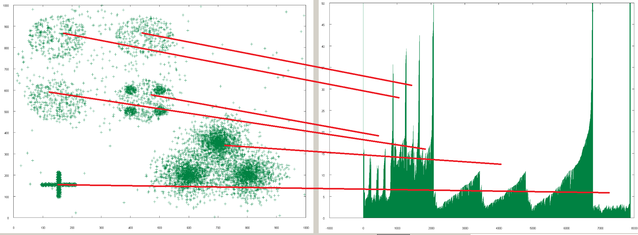
Figure 1: OPTICS reachability plot (right) of a sample database (left) consisting of clusters with different shape, size and density. The correspondence is denoted by red lines: note that clusters correspond to concave regions on the right, and hierarchical clusters are also clearly visible on the reachability plot: shallower regions containing deeper concavities correspond to hierarchical clusters.

As a side effect, OPTICS reduces the dimensionality of the input dataset; combining OPTICS with the visualization method proposed later can be thus also used to visually compare two hierarchical clusterings of (possibly) multi-dimensional datasets. The literature of dimension reduction and visualization of high-dimensional data sets is quite rich (e.g. VIS-EXAMPLE1 ), which is also true for visualizing hierarchical clusterings (e.g. VIS-EXAMPLE2 ). Our method combines dimension reduction with visualization, making it possible to compare clustering results to an a-priori given hierarchical classification without assigning objects to specific clusters.

3 Colouring nodes of the a priori-known hierarchical data structure

In the visualization phase we are going to assign colours to each entry occurring on the x-axis of the OPTICS reachability plot, based on the a-priori given hierarchical classification of these objects. The main idea is that we would like to use similar colours on entries that belong to ”similar” classes in the a priori-known hierarchical data structure. As this hierarchical structure can be conveniently represented by a (non-binary) tree (a dendogram), our aim is to assign colours to tree nodes so that nodes having a short path between them (i.e. their common ancestor is close to them) are assigned similar colours. We would also like to achieve that the depth of a given node in this tree is somehow reflected in its colour.

We will use the HSB (Hue, Saturation, Brightness) representation of colours. HSB coordinates can easily be converted to RGB (Red, Green, Blue) colour coordinates. As an example, it is easy to see that points of the whole Hue scale may be assigned to leaf nodes with full Saturation and Brightness, while the root node may be coloured black. It is also straightforward to use Saturation and Brightness as an indicator of depth (distance from root) in the tree. This is the main motivation of the chosen HSB colour coordinate system.

More precisely, assignment of colours to the a-priori given dendogram is carried out as follows.

3.1 Determining Saturation and Brightness

Saturation and Brightness assigned to a given tree node will be (not necessarily directly) proportional to the level (distance from root) of this particular node. The level of each node can be – for instance – determined by BFS (Breadth-First Search) algorithm starting from the root. The root itself will always be black and nodes on the lower levels will be ”more colourful” – see Figure 3.

3.2 Determining Hue

Let us call a tree node with no children a leaf. Let $C^{t}_{k}$ denote the $k$-th child of tree-node $t$ (we may define an arbitrary ordering on child nodes). Let the the weight of a leaf $l$ be $W(l)=1$, and the weight of a given node $t$ having $c$ children be the number of nodes its subtree contains, or (given by a recursive definition):

$$W(t)=1+\sum_{k=1}^{c}W(C^{k}_{t}).$$ (1)

Each node $t$ is assigned a closed hue interval $I(t)=[I^{t}_{l},I^{t}_{r}]$; let us denote the size of $I(t)$ with $S(t)=I^{t}_{r}-I^{t}_{l}$. The root of the tree is assigned the whole hue interval $I(root)=[0;1]$. The hue assigned to any node $t$ is $H(t)=\frac{I^{t}_{l}-I^{t}_{r}}{2}$ (e.g. $H(root)=0.5$).

The children of node $t$ are assigned non-overlapping subintervals of $I(t)$ that are separated from each other. The latter means that a certain part of $I(t)$ is not used at all at any child of $t$; this unused part provides separator intervals to ensure that Hues are highly distinct between nodes with different ancestors (this is the motivation of using such separator intervals). Let us denote the proportion of this unused hue interval to $S(t)$ with $E$ (which is a global parameter of the colouring method).

A certain part of $I(t)$ is divided between the children of $t$. The size of the hue interval assigned to the $k$-th child of $t$, $S(C^{t}_{k})$ is

$$S(C^{t}_{k})=\frac{W(C^{t}_{k})}{W(t)-1}\cdot(1-E)\cdot S(t).$$ (2)

In other words this means that we take the interval belonging to node $t$ with size $S(t)$, and assign an $(1-E)$-proportion of this interval to child nodes’ hue intervals, and an the remaining will be used to provide separator intervals that are not assigned to any descendant of $t$. Sizes of assigned hue intervals are proportional to the weight of the given child node.

We would now like to formulate the hue interval belonging to the $C^{t}_{k}$. Let $c$ denote the number of children of node $t$. The $c$ hue intervals determined for each child node $t$ are separated by $c-1$ separator-intervals, each sized $\frac{E\cdot S(t)}{c-1}$. Taking into account that the hue interval belonging to the $k$-th child is preceded by $k-1$ equal-sized separators and $k-1$ hue intervals belonging to the previous $k-1$ children,

$$I(C^{t}_{k})=\left[(k-1)\cdot\frac{E\cdot S(t)}{c-1}\cdot\sum\limits_{i=1}^{k-1}S(C^{t}_{k})\;;\;\;(k-1)\cdot\frac{E\cdot S(t)}{c-1}\cdot\sum\limits_{i=1}^{k}S(C^{t}_{k})\right].$$ (3)

To illustrate the above principles, we provide two simple examples. If we set $E=\frac{1}{3}$ and use a balanced binary tree to be coloured, the hue intervals occurring at each level of the tree will converge to the Cantor set if we move farther and farther from the root (see Figure 2).

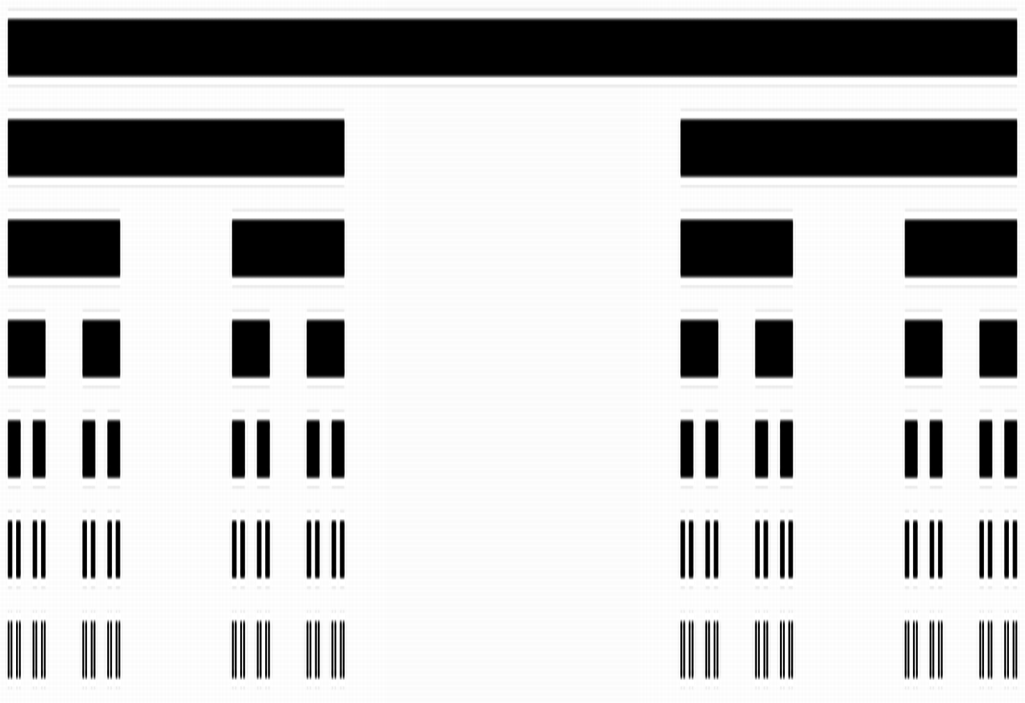
Figure 2: Illustration of the sizes of Hue intervals occurring on the levels of a binary tree ($E=\frac{1}{3}$, the $i$-th level has $2^{i}$ nodes) (Source: http://en.wikipedia.org/wiki/Cantor_set, downloaded January 7, 2012).

In Figure 3, a small tree consisting of 24 nodes is depicted. The tree nodes are coloured according to the principle described: each node is recursively assigned a Hue interval that is proportional to its weight; Hue assigned to a given tree node equals to the middle of this interval; Saturation and Brightness is proportional to the distance from the root. Each node is labelled by its weight (see Equation eq:TreeColouring1). $E=0.2$.

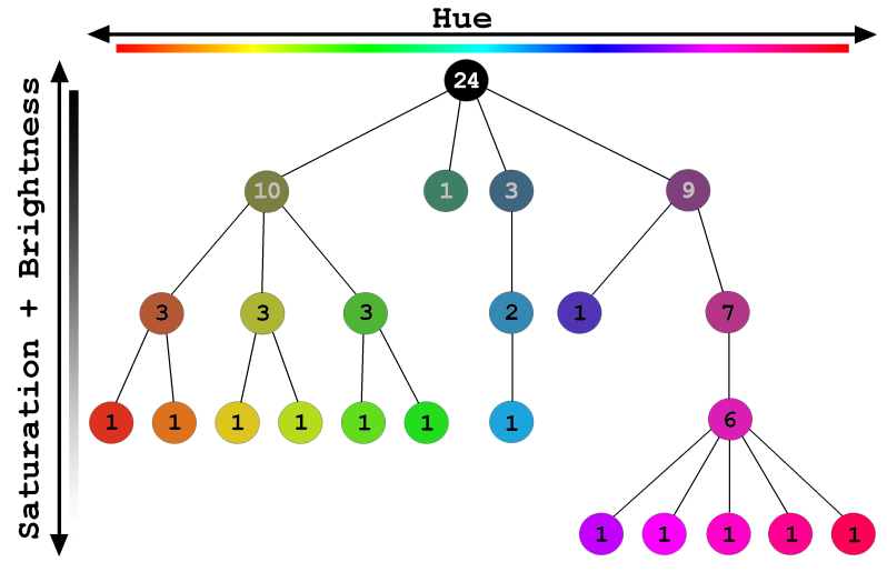
Figure 3: Illustration of the proposed tree-colouring principle on a sample tree consisting of 24 nodes. The numbers written in the nodes are the weights assigned.

4 Results

4.1 Example 1.: Sequence-based clustering the SwissProt database – verification based on NCBI taxonomy identifiers

We applied the OPTICS algorithm to 389046 amino acid sequences occurring in SwissProt release 55.1. In this case, the distance measure for two objects (amino acid sequences) was based on local sequence similarity. Our goal was to visualize the species-composition of potential clusters. To achieve this, we used the NCBI taxonomy hierarchy (which is essentially a tree) as an a-priori given hierarchical classification, restricted it to the taxonomy identifiers occurring in SwissProt, and coloured the resulting taxonomy-tree using the method proposed. As an example, the first two levels of the NCBI taxonomy hierarchy is shown on Figure 4 with a possible colouring.

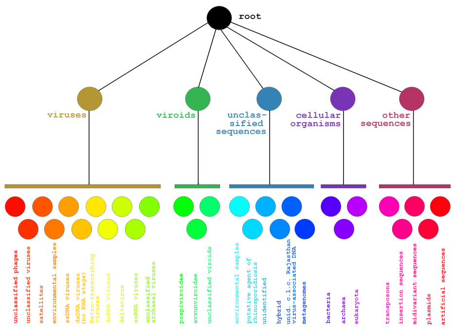
Figure 4: Upper two levels of the NCBI taxonomy tree coloured by the proposed method. Note that the colours will be different when colouring the whole tree, as nodes on level 2 are going to have quite different weights.

Due to size limitations (the x-axis of the full reachability plot consists of the 389046 sequences being clustered), viewing the coloured reachability plot is quite a challenge. A small, yet illustrative chunk (width: 700 sequences) of the reachability plot is shown in Figure 5. On the other hand, the annotated reachability plot of the first 20000 sequences can also be viewed on the author’s home page:
http://www.cs.elte.hu/$\sim$hugeaux/swissclust/swissclust_optics_M004_No001.html

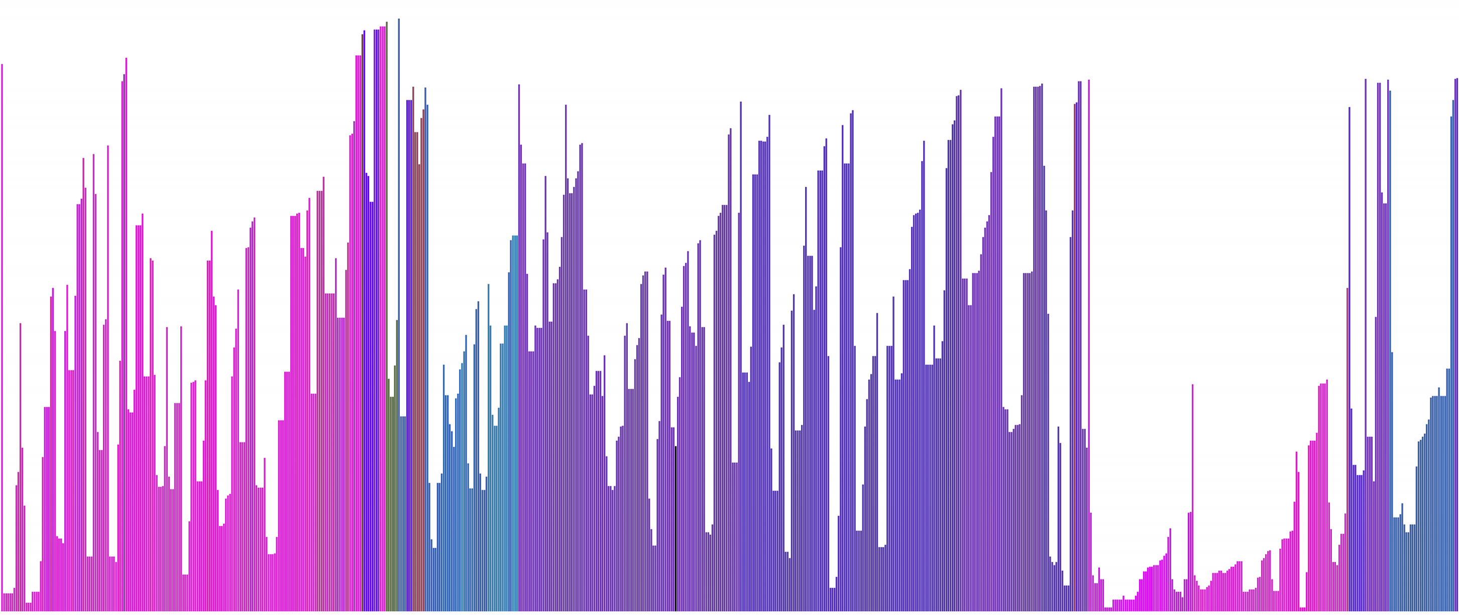
Figure 5: The reachability plot of 700 sequences chosen from SwissProt, coloured by their species

4.2 Example 2.: Clustering locations of specific atoms in the serine protease enzyme family – verification based on SCOP classification

In a previous study by Ivan et al. Ivan2009 , strong correlation has been shown to exist between the enzymatic function of serine proteases and the orientation of amino acid side chains constituting the ”catalytic machinery” of the enzyme. The method described heavily depends on the OPTICS algorithm combined with the hereby proposed visualization technique. The main hypothesis was that some specific families of serine proteases can be distinguished solely by taking the coordinates of four specific atoms per protein (thus assigning a 12-dimensional feature vector to each enzyme), and clustering these feature vectors by the OPTICS algorithm (based on Euclidean distance as a similarity measure). The entries (enzymes represented by their PDB Berman2003 codes) were colored on the OPTICS reachability plot by the SCOP Murzin1995 classification of the proteins. SCOP is a 7-level hierarchical classification of three-dimensional protein structures; a given amino acid range of a PDB entry belongs to exactly one SCOP class on each level of this hierarchy. Traversing the SCOP tree from the root to a given amino acid range of a PDB entry (a leaf), one can obtain more and more precisely defined classes the given entry belongs to. Levels of the SCOP tree are named

• Root (level 0)

• Class (level 1)

• Fold (level 2)

• Superfamily (level 3)

• Family (level 4)

• Protein (level 5)

• Species (level 6).

The domains – amino acid ranges – that are classified are located on level 7.

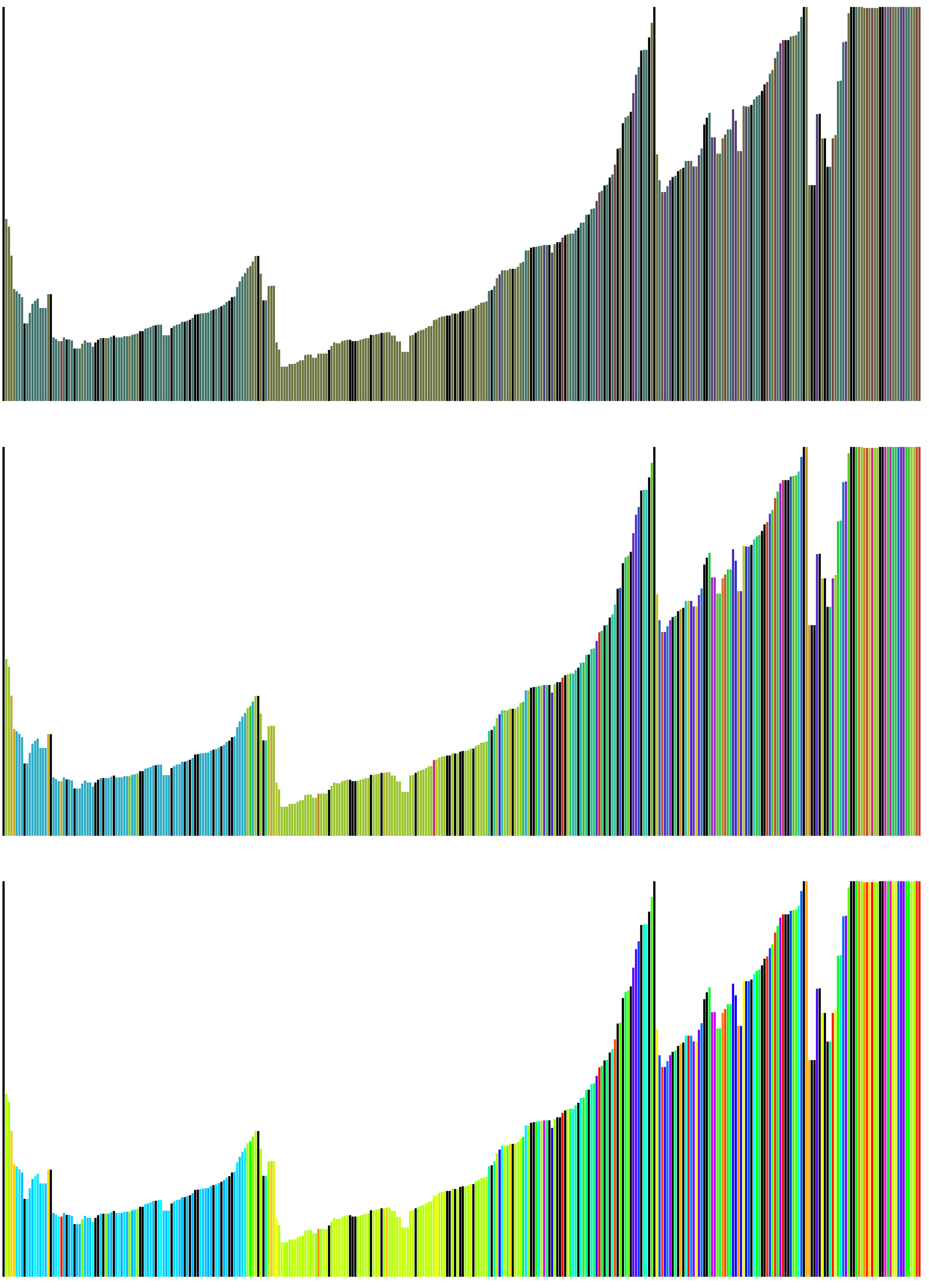
Figure 6: The reachability plot of 350 PDB entries coloured by their SCOP classification. Entries coloured black have no known SCOP classification. Focus of this work is described in Ivan2009 .

In order to visualize the assumed correlation between feature vector similarity and SCOP classification, the 7-level SCOP hierarchy has been coloured by the visualization method described. The two main homogenously coloured regions on the reachability plot indicate proteins belonging to similar SCOP classes (see Figure 6). The upper-panel reachability plot in Figure 6 is coloured by the entries’ SCOP ’Class’ (level 1 in SCOP tree); the reachability plot in the middle panel of Figure 6 is coloured by the entries’ SCOP ’Superfamily’ (level 3 in SCOP tree), and the lower-panel reachability plot in Figure 6 is coloured by the entries’ SCOP ’Protein’ (level 5 in SCOP tree).

It can be seen very clearly that moving away from the root of SCOP (i.e., from the upper panel to the lower panel on Figure 6, that is, from colouring according to level 1 in the SCOP tree through the colouring by level 5 in SCOP tree at the bottom panel), colours become more saturated, and, additionally, more and more details become visible due to subtle changes in the entries’ colours, witnessing that specific families of serine proteases can be distinguished solely by taking the coordinates of four specific atoms per protein.

5 Conclusion

We proposed a method capable of visualizing connection between an a priori given classification and the OPTICS clustering algorithm’s output for a given set of input objects. We have shown how this method can be used to investigate correlations between clustering results and a-priori available knowledge, and also cited an example of how the method can be used to help validating hypotheses in two bioinformatics-related tasks. We demonstrated that the presented method is capable to visualize the correlation of the a-priori available knowledge and the knowledge gained from clustering.

References

- (1) M. Ankerst, M. M.Breunig, H. Kriegel, and J. Sander. Optics: Ordering points to identify the clustering structure. In Proc. ACM SIGMOD ’99 Int. Conf. on Management of Data, Philadelphia PA, 1999.
- (2) C. L. Bentley and M. O. Ward. Animating multidimensional scaling to visualize n-dimensional data sets. In Proceedings of Information Visualization, pages 72–73, 1996.
- (3) Helen Berman, Kim Henrick, and Haruki Nakamura. Announcing the worldwide protein data bank. Nat Struct Biol, 10(12):980, Dec 2003.
- (4) A. Fiser and B. G. Vertessy. Altered subunit communication in subfamilies of trimeric dutpases. Biochem Biophys Res Commun, 279(2):534–542, Dec 2000.
- (5) Joana P Goncalves, Yves Moreau, and Sara C Madeira. Alibimotif: integrating alignment and biclustering to unravel transcription factor binding sites in dna sequences. Int J Data Min Bioinform, 6(2):196–215, 2012.
- (6) Gabor Ivan and Vince Grolmusz. When the web meets the cell: using personalized pagerank for analyzing protein interaction networks. Bioinformatics, 27(3):405–407, Feb 2011.
- (7) Gabor Ivan, Zoltan Szabadka, and Vince Grolmusz. Being a binding site: Characterizing residue composition of binding sites on proteins. Bioinformation, 2(5):216–221, 2007.
- (8) Gabor Ivan, Zoltan Szabadka, and Vince Grolmusz. A hybrid clustering of protein binding sites. FEBS J, 277(6):1494–1502, Mar 2010.
- (9) Gabor Ivan, Zoltan Szabadka, Rafael Ordog, Vince Grolmusz, and Gabor Naray-Szabo. Four spatial points that define enzyme families. Biochem Biophys Res Commun, 383(4):417–420, Jun 2009.
- (10) Andrew V Kossenkov and Michael F Ochs. Matrix factorisation methods applied in microarray data analysis. Int J Data Min Bioinform, 4(1):72–90, 2010.
- (11) Jeffrey D Leblond, Andrew D Lasiter, Cen Li, Ramiro Logares, Karin Rengefors, and Terence J Evens. A data mining approach to dinoflagellate clustering according to sterol composition: correlations with evolutionary history. Int J Data Min Bioinform, 4(4):431–451, 2010.
- (12) Ross K K Leung and Stephen K W Tsui. imowse, a scoring scheme bridging in silico and in vitro digestion in pmf. Int J Data Min Bioinform, 6(1):104–113, 2012.
- (13) A. G. Murzin, S. E. Brenner, T. Hubbard, and C. Chothia. Scop: a structural classification of proteins database for the investigation of sequences and structures. J Mol Biol, 247(4):536–540, Apr 1995.
- (14) Rafael Ordog, Zoltan Szabadka, and Vince Grolmusz. Analyzing the simplicial decomposition of spatial protein structures. BMC Bioinformatics, 9(S11), 2008.
- (15) DarĂo Rojas, Luis Rueda, Alioune Ngom, Homero Hurrutia, and Gerardo Carcamo. Image segmentation of biofilm structures using optimal multi-level thresholding. Int J Data Min Bioinform, 5(3):266–286, 2011.
- (16) Zoltan Szabadka and Vince Grolmusz. High throughput processing of the structural information in the protein data bank. J Mol Graph Model, 25(6):831–836, Mar 2007.
- (17) B. G. Vertessy, P. Zalud, P. O. Nyman, and M. Zeppezauer. Identification of tyrosine as a functional residue in the active site of Escherichia coli dUTPase. Biochim Biophys Acta, 1205(1):146–150, Mar 1994.
- (18) G. J. Wills. An interactive view for hierarchical clustering. In Proceeding of Information Visualization, pages 26–31, 1998.
- (19) Qiaofeng Yang and Stefano Lonardi. A parallel edge-betweenness clustering tool for protein-protein interaction networks. Int J Data Min Bioinform, 1(3):241–247, 2007.
- (20) Li-Juan Zhang, Zhou-Jun Li, and Huo-Wang Chen. Handling gene redundancy in microarray data using grey relational analysis. Int J Data Min Bioinform, 2(2):134–144, 2008.