Sensitivity to the Single Production of Vector-Like Quarks at an Upgraded Large Hadron Collider

Abstract

In this note we consider the sensitivity of the Large Hadron Collider (LHC) to the single production of new heavy vector-like quarks. We consider a model with large mixing with the standard model top quark with electroweak production of single heavy top quarks. We consider center of mass energies of 14, 33, and 100 TeV with various pileup scenarios and present the expected sensitivity and exclusion limits.

1 A benchmark model for vector-like quarks

Vector-like quarks (VLQs)  [1] are a general prediction of a wide class of beyond the Standard Model theories, as extra dimensions, composite Higgs models (see [2, 3, 4, 5, 6, 7, 8] for recent studies on VLQs in these frameworks), Little Higgs [9, 10] and top-coloron models [11].
We will consider as a benchmark model to describe the VLQ phenomenology a two-site description that reproduces the low-energy limit of a large set of composite Higgs models (CHM) [12] and warped extra-dimensional theories with a custodial symmetry in the bulk [13].
CHMs are compelling theories of new physics. They give an explanation of the EWSB by considering that it is triggered by a new strong dynamics, with a scale of compositeness of several TeVs. The Higgs is a field of the composite sector. Because of its composite nature, its mass is protected from radiative corrections above the compositeness scale and is further protected if it is also the pseudo-Goldstone boson of some symmetry breaking in the strong sector [14]. In this case the Higgs can be naturally much lighter than the other resonances from the strong sector (which have masses of the TeV order). A crucial role in this mechanism is played by the top-partner VLQs, arising from the strong sector, which intervene in cutting-off the top-loop contribution to the Higgs mass.
The two building blocks of the effective theory we will consider are the weakly-coupled sector of the elementary fields and the composite sector, that comprises the Higgs. The two sectors are linearly coupled to each other through mass mixing terms [15]. After diagonalization, the elementary/composite basis rotates to the mass eigenstate one, made of SM and heavy states, among which the VLQs, that are admixture of elementary and composite modes. A minimal model, which incorporates the custodial symmetry and the Left-Right parity needed for CHM to pass the EWPT [16] and which includes the full set of resonances which are needed to generate the top-quark mass is that where composite fermions fill a 5 of $SO(5)$. This same description has been adopted in [17, 18, 4].
The composite sector has a global symmetry $SO(4)\times U(1)_{X}\sim SU(2)_{L}\times SU(2)_{R}\times U(1)_{X}$ and includes the Higgs

$${\cal H}=(\mathbf{2},\mathbf{2})_{0}=\begin{bmatrix}\phi_{0}^{\dagger}&\phi^{+}\\ -\phi^{-}&\phi_{0}\end{bmatrix}\,,$$ (1)

and the following set of VLQs:

$$\begin{split}&\mathcal{Q}=\left[\begin{array}[]{cc}T&T_{5/3}\\ B&T_{2/3}\end{array}\right]=\left(\mathbf{2},\mathbf{2}\right)_{2/3}\ ,\ \tilde{T}=\left(\mathbf{1},\mathbf{1}\right)_{2/3}\end{split}$$ (2)

namely, a weak singlet, $\tilde{T}$, partner of $t_{R}$, and two weak doublets, $(T,B)$, partner of $(t_{L},b_{L})$, and $(T_{5/3},T_{2/3})$, the doublet of exotic quarks which have no direct mixing with the top. These latter, which are generally named ‘custodians’, can be much lighter than the other VLQs in the limit case of a fully composite $t_{L}$. The elementary sector has the same particle content of the SM without the Higgs. The $SU(2)_{L}\times U(1)_{Y}$ elementary fields gauge the corresponding global invariance of the composite sector, with $Y=T_{R}^{3}+X$.
The Lagrangian that describes our model (in the gauge-less limit) reads:

$${\cal L}= \,{\cal L}_{elementary}+{\cal L}_{composite}+{\cal L}_{mixing}$$ (3)

$${\cal L}_{elementary}= \,\bar{q}_{L}i\!\not\!\partial\,q_{L}+\bar{t}_{R}i\!\not\!\partial\,t_{R}$$ (4)

$${\cal L}_{composite}= \ \text{Tr}\left\{\bar{\mathcal{Q}}\left(i\not\!\partial-M_{Q*}\right)\mathcal{Q}\right\}+\text{Tr}\left\{\bar{\tilde{T}}\left(i\not\!\partial-M_{\tilde{T}*}\right)\tilde{T}\right\}$$ (5)

$$+\frac{1}{2}\,\text{Tr}\left\{\partial_{\mu}{\cal H}^{\dagger}\partial^{\mu}{\cal H}\right\}-V({\cal H}^{\dagger}{\cal H})+Y_{*}\text{Tr}\left\{\bar{\mathcal{Q}}\mathcal{H}\right\}\tilde{T}$$ (6)

$$\begin{split}{\cal L}_{mixing}=&-\Delta_{L}\bar{q}_{L}\left(T,B\right)-\Delta_{R}\bar{t}_{R}\tilde{T}+h.c.\end{split}$$ (7)

where $V({\cal H}^{\dagger}{\cal H})$ is the Higgs potential.
${\cal L}^{YUK}=Y_{*}\text{Tr}\left\{\bar{\mathcal{Q}}\mathcal{H}\right\}\tilde{T}$ describes the Yukawa interactions among Higgs and composite fermions. The Yukawa coupling $Y_{*}$ is large, $1<Y_{*}\ll 4\pi$, where $4\pi$ marks out the non-perturbative regime. $Y_{*}$ values greater than 3 are generally preferred by electoweak precision tests (for smaller $Y_{*}$ values the theory also predict lighter vector resonances that would give somehow large corrections to the S parameter [19]).
The two-site Lagrangian (3) can be diagonalized by a field rotation parametrized by:

$$\tan\varphi_{tR}=\frac{\Delta_{R}}{M_{\tilde{T}*}}\equiv\frac{s_{R}}{c_{R}},\qquad\tan\varphi_{L}=\frac{\Delta_{L}}{M_{Q*}}\equiv\frac{s_{L}}{c_{L}}$$ (8)

Where $\sin\varphi_{tR}$ (shortly indicated as $s_{R}$) and $\sin\varphi_{L}$ ($s_{L}$) respectively represent the degree of compositeness of $t_{R}$ and $(t_{L},b_{L})$. After the diagonalization of the elementary/composite mixing, the Yukawa Lagrangian for SM and heavy fields reads:

$$\begin{split}\mathcal{L}^{YUK}=&+Y_{*}s_{L}c_{R}\left(\bar{t}_{L}\phi^{{\dagger}}_{0}\tilde{T}_{R}-\bar{b}_{L}\phi^{-}\tilde{T}_{R}\right)-Y_{*}s_{R}\left(\bar{T}_{2/3L}\phi_{0}t_{R}+\bar{T}_{5/3L}\phi^{+}t_{R}\right)\\ &-Y_{*}c_{L}s_{R}\left(\bar{T}_{L}\phi^{{\dagger}}_{0}t_{R}-\bar{B}_{L}\phi^{-}t_{R}\right)+Y_{*}s_{L}s_{R}\left(\bar{t}_{L}\phi^{{\dagger}}_{0}t_{R}-\bar{b}_{L}\phi^{-}t_{R}\right)\\ &+\ h.c.+\ \dots\\ \end{split}$$ (9)

After the EWSB, the top-quark mass is generated, $m_{t}=\frac{v}{\sqrt{2}}Y_{*}s_{L}s_{R}$. The induced electroweak mixing among fermions also generates effective couplings of the VLQs with a SM quark and a weak boson. These effective couplings determine the VLQ decays and allow for the VLQ single production.
The rates for the VLQ ($\chi$) decays into a weak boson and a SM quark ($\psi$) read:

$$\begin{split}&\Gamma\left(\chi\rightarrow W_{L}\psi\right)=\frac{\lambda^{2}_{W\chi}}{32\pi}M_{\chi}\left[\left(1+\frac{m^{2}_{\psi}-M^{2}_{W}}{M^{2}_{\chi}}\right)\left(1+\frac{m^{2}_{\psi}+2M^{2}_{W}}{M^{2}_{\chi}}\right)-4\frac{m^{2}_{\psi}}{M^{2}_{\chi}}\right]\sqrt{1-2\frac{m^{2}_{\psi}+M^{2}_{W}}{M^{2}_{\chi}}+\frac{\left(m^{2}_{\psi}-M^{2}_{W}\right)^{2}}{M^{4}_{\chi}}}\\ &\Gamma\left(\chi\rightarrow Z_{L}\psi\right)=\frac{\lambda^{2}_{Z\chi}}{64\pi}M_{\chi}\left[\left(1+\frac{m^{2}_{\psi}-M^{2}_{Z}}{M^{2}_{\chi}}\right)\left(1+\frac{m^{2}_{\psi}+2M^{2}_{Z}}{M^{2}_{\chi}}\right)-4\frac{m^{2}_{\psi}}{M^{2}_{\chi}}\right]\sqrt{1-2\frac{m^{2}_{\psi}+M^{2}_{Z}}{M^{2}_{\chi}}+\frac{\left(m^{2}_{\psi}-M^{2}_{Z}\right)^{2}}{M^{4}_{\chi}}}\\ &\Gamma\left(\chi\rightarrow h\psi\right)=\frac{\lambda^{2}_{h\chi}}{64\pi}M_{\chi}\left(1+\frac{m^{2}_{\psi}}{M^{2}_{\chi}}-\frac{M^{2}_{h}}{M^{2}_{\chi}}\right)\sqrt{\left(1-\frac{m^{2}_{\psi}}{M^{2}_{\chi}}+\frac{M^{2}_{h}}{M^{2}_{\chi}}\right)^{2}-4\frac{M^{4}_{h}}{M^{4}_{\chi}}}\ .\end{split}$$ (10)

The effectice vertices $\lambda_{W/Z/h\chi}$, that can be directly extracted from the Yukawa Lagrangian in (9), are, for the different VLQs:

	$T$	$B$	$T_{2/3}$	$T_{5/3}$	$\tilde{T}$
$\chi\to W\psi$	$0$	$Y_{*}c_{L}s_{R}$	$0$	$Y_{*}s_{R}$	$Y_{*}s_{L}c_{R}$
$\chi\to Z\psi$	$Y_{*}c_{L}s_{R}$	$0$	$Y_{*}s_{R}$	$0$	$Y_{*}s_{L}c_{R}$
$\chi\to h\psi$	$Y_{*}c_{L}s_{R}$	$0$	$Y_{*}s_{R}$	$0$	$Y_{*}s_{L}c_{R}$

The above expressions are calculated by diagonalizing the mixing among fermions at first order in

$$\sin\theta_{\chi}=\frac{\lambda_{\chi}v}{\sqrt{2}M_{\chi}}\ ,$$ (11)

which parametrizes the superposition of a VLQ $\chi$ with the top. We expect corrections of $\mathcal{O}(1)$ in the VLQ decay rates and in the VLQ single production cross sections, for $\lambda_{\chi}v/(\sqrt{2}M_{\chi})\simeq 1$.

Since VLQs are essentially composite states which couple strongly to composite modes and thus to longitudinally polarized weak bosons and to the Higgs, their branching-ratios are basically fixed by the equivalence theorem. One finds, approximately

	$T$	$B$	$T_{2/3}$	$T_{5/3}$	$\tilde{T}$
$BR[\chi\to W\psi]$	$0$	$1$	$0$	$1$	$0.5$
$BR[\chi\to Z\psi]$	$0.5$	$0$	$0.5$	$0$	$0.25$
$BR[\chi\to h\psi]$	$0.5$	$0$	$0.5$	$0$	$0.25$

Fig. 1 shows the decay branching-ratios and the total decay width for $\tilde{T}$. VLQ total decay widths depend quadratically on the effective vertices $\lambda_{\chi}$.

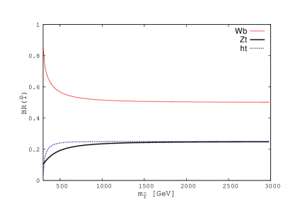
Figure 1: BRs (Left Plot) and total decay width (Right Plot) of $\tilde{T}$. The width depends quadratically on $\lambda_{\tilde{T}}$; the continuous line in the Right Plot refers to $\lambda_{\tilde{T}}=3$, the dotted lines define a range of variation $2<\lambda_{\tilde{T}}<4$ of the total decay width.

The flavor structure of the two-site model here described has been analyzed in [20, 21, 22, 23]. In the anarchic scenario for the flavor of the composite sector, where $Y_{*}$ is a matrix in the flavor space with elements all of the same size, flavor observables like $\epsilon_{K}$ and $\epsilon^{{}^{\prime}}/\epsilon_{K}$ place strong constraints on the CHM spectrum. Recent studies [21, 24] have shown that the flavor constraints on VLQ masses can be lowered to the order of 1 TeV or below if a $U(2)^{3}$ flavor symmetry is present in the composite sector, instead of the anarchic flavor structure. In this case, VLQs couple strongly to third-generation quarks and weakly to light quarks, thus reflecting the same VLQ phenomenology above described.

2 VLQ production mechanisms

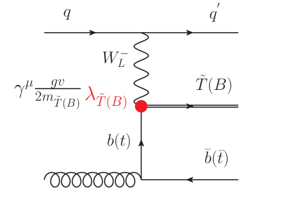
Figure 2: Single production of top- and bottom- prime VLQs.

Figure 3: VLQ cross sections at the 33 TeV LHC. Dotted curves correspond to single-productions for $\lambda_{\chi}=3$.

VLQs can be produced at the LHC in pairs, the dominant mode is via gluon-gluon fusion, or singly, by means of their electroweak effective couplings to a weak boson and a SM quark (Fig. 2). These latter production mechanisms have larger rates than those of pair productions for heavier VLQs. Moreover, analyses of single-production channels might permit the measurement of the effective couplings $\lambda_{\chi}$. Fig. 3 shows the cross sections at the 33 TeV LHC for VLQ pair production and for single production of $\tilde{T}$ and $B$ (the same for $T_{5/3}$), for $\lambda_{\chi}=3$. The $\tilde{T}$ single-production, that proceeds via the intermediate exchange of a bottom quark , has a rate significantly higher than those of $B$ and $T_{5/3}$ single productions, which are mediated by the exchange of a top.

3 Simulation

In order to evaluate the sensitivity , samples were generated using the DELPHES [28] fast detector simulation using the generic “Snowmass Detector” parameters [25]. The background samples were generated in bins of $H_{T}$, as described in [26]. The signal samples were produced using the model from one of the authors in Ref [4] as described in the Section 1.

The following scenarios were considered:

• Three scenarios at $\sqrt{s}$= 14 TeV, with an average of 0, 50, and 140 pileup events with an integrated luminosity of 3000 $\rm fb^{-1}$.

• Three scenarios at $\sqrt{s}$ = 30 TeV, with an average of 0, 50, and 140 pileup events with an integrated luminosity of 3000 $\rm fb^{-1}$.

• Three scenarios at $\sqrt{s}$ = 100 TeV, with an average of 0, 50, and 140 pileup events with an integrated luminosity of 3000 $\rm fb^{-1}$.

4 Channels Considered

As mentioned in Section 1 , the heavy like top quark can decay into one of three modes:

• T $\rightarrow$ Wb

• T $\rightarrow$ tZ

• T $\rightarrow$ tH

In this note we consider the later two decay modes.

4.1 T $\rightarrow$ tH

In this decay mode we focus on the decay of the Higgs to its most frequent decay into $b\bar{b}$ and the case where the top quark decays semi-leptonically into a charged lepton, neutrino and b-quark. We reconstruct the heavy VLQ in a series of steps. First we select events based on the decay topology:

• Events are required to have one lepton (muon or electron) with $|\eta|<$ 2.5

• Events are required to have missing transverse energy greater than 30 GeV

• Events are required to have at three jets that have $p_{T}>$ 25 GeV that are identified as b-jets

• Events are required to have two jets with $|\eta|>$ 3.0 (from the forward scattered quarks from the hard subprocess)

• Events are required to have $H_{T}>$ 750 GeV

Events are then reconstructed in the following manner. The charged lepton and the neutrino are assumed to come from the W boson in the decay. We measure the complete four-vector of the charged lepton but only can assume the two transverse components of the missing transverse energy are from the two transverse components of the neutrino. Since we are missing the longitudinal component of the neutrino momentum we must make some assumption to completely reconstruct the event. We force the invariant mass of the missing transverse momentum and the charged lepton to that of the pole mass of the W. This allows for us to solve for the longitudinal component of the neutrino momentum. This is a quadratic equation and leads to up to two real solutions. In the case of two solutions we take the solution which minimizes the angle between the charged lepton and the neutrino.

After reconstruction of the top quark candidate in the event we make the following additional requirements:

• The $\Delta$ R between the lepton and the b-jet used for the top reconstruction must be larger than 0.7

• One Cambridge-Achen jet must have an invariant mass between 100-150 GeV

We utilize the entire Snowmass background samples to estimate the background but by far the largest contribution is standard model $t\bar{t}$ production.

5 T $\rightarrow$tZ

For the tZ channel we focus on the signal with the lowest background and select trilepton events. In this decay mode we focus on the decay of the $Z$ boson into leptons and the case where the top quark decays semi-leptonically into a charged lepton, neutrino and b-quark.

The reconstructed objects used for the analysis are selected as following:

• Jets are reconstructed using the anti$-k_{t}$ algorithm with $r=0.5$. They are required to have $p_{T}>$higher than 30 $\mathrm{GeV}$and $|\eta|<$ 5.0. Jets must be isolated, therefore an overlap removal between jets is applied, in $\Delta R<0.5$: the jet with the higest $p_{T}>$is retained and the other discarded.

• Leptons (muons or electrons) are required to have $p_{T}>$higher than 20 $\mathrm{GeV}$and $|\eta|<$ 2.5. Furthermore they are required to be isolated from jets, within $\Delta R<0.5$.

A b-tagging algorithm is also available to identify jets coming from a b-quark.

We reconstruct the heavy VLQ in a series of steps. First we select events based on the decay topology:

• Events are required to have exactly three leptons

• Events are required to have at least one light jet (not b-tagged)

• Events are required to have at least two b-tagged jets

• Events are required to have missing transverse energy greater than 30 $\mathrm{GeV}$

The event reconstruction in this case is a bit simpler than the $Ht$ case.

First of all, the $Z$ boson candidate is reconstructed from a pair of same flavor leptons and a cut on the invariant mass of the two leptons is applied. If in the events there are only two leptons with the same flavor (two electrons and a muon or viceversa), the two same flavor leptons are required to form an invariant mass within a 10 $\mathrm{GeV}$window of the mass of the $Z$ boson. If instead the three leptons have all the same flavor, the couple with the invariant mass closer to the $Z$ boson mass are considered for the 10 $\mathrm{GeV}$window mass cut.

After reconstructing the $Z$ boson, the light jet from the forward scattered quarks from the hard subproces is looked for. The light jet with the highest $\eta$ is selected and this jet is required to have $|\eta|>2.5$.

The top candidate is reconstructed using the same method as described in the previous section, by using the third lepton in the event and the b-tagged jet that best reproduces the top mass. Furthermore a cut on the mass of the $Wj$ is applied: $160\mbox{$\mathrm{GeV}$}<m_{Wj}<190\mbox{$\mathrm{GeV}$}$.

Again we utilize the entire Snowmass background samples to estimate the background. The samples with the largest contributions come from diboson production and top quark pair production associated with a boson production.

6 Cross-Sections and Event Yields

In Table LABEL:tab:sig and 9 the cross sections for the signal and the main backgrounds respectively are reported, for the three center of mass energies considered in this study.

7 Results

The expected significances for the combination of both channels is shown in Figure  4.

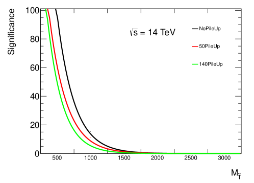
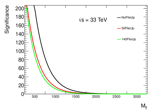
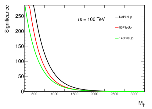
Figure 4: Expected Significance at center of mass energies 14 (top left), 33 (top right), and 100 (bottom) GeV with no pileup, 50 interaction, and 140 interactions  .

Appendix A Signal Cross Sections

Center of	Lambda	Decay	Mass	Width	Cross
Mass Energy [TeV]			[GeV]	[GeV]	Section [pb]
100	3	Zt	500	78.6	117.104966
100	3	Zt	1000	173.6	10.877649
100	3	Zt	1500	264.9	2.237840
100	3	Zt	2000	355.4	0.675062
100	3	Zt	2500	445.4	0.254231
100	3	Zt	3000	535.3	0.110822
33	3	Zt	500	78.6	17.296388
33	3	Zt	1000	78.6	2.113275
33	3	Zt	1500	173.6	0.257407
33	3	Zt	2000	264.9	0.057440
33	3	Zt	2500	355.4	0.016986
33	3	Zt	3000	535.3	0.005486
14	3	Zt	500	78.6	2.573795
14	3	Zt	1000	173.6	0.111849
14	3	Zt	1500	264.9	0.011920
14	3	Zt	2000	355.4	0.001939
14	3	Zt	2500	445.4	0.000402
14	3	Zt	3000	535.3	0.000098

Table 1: Generated Masses, Widths and Cross Sections for top partner single production decaying into $Zt$.

Center of	Lambda	Decay	Mass	Width	Cross
Mass Energy [TeV]			[GeV]	[GeV]	Section [pb]
100	3	Wb	500	78.6	318.691708
100	3	Wb	1000	173.6	23.474201
100	3	Wb	1500	264.9	4.624145
100	3	Wb	2000	355.4	1.371373
100	3	Wb	2500	445.4	0.513678
100	3	Wb	3000	535.3	0.223635
33	3	Wb	500	78.6	47.820304
33	3	Wb	1000	78.6	5.122861
33	3	Wb	1500	173.6	0.540823
33	3	Wb	2000	264.9	0.117806
33	3	Wb	2500	355.4	0.034511
33	3	Wb	3000	535.3	0.011076
14	3	Wb	500	78.6	7.276922
14	3	Wb	1000	173.6	0.244653
14	3	Wb	1500	264.9	0.024868
14	3	Wb	2000	355.4	0.003980
14	3	Wb	2500	445.4	0.000819
14	3	Wb	3000	535.3	0.000198

Table 2: Generated Masses, Widths and Cross Sections for top partner single production decaying into $Wb$.

Center of	Lambda	Decay	Mass	Width	Cross
Mass Energy [TeV]			[GeV]	[GeV]	Section [pb]
100	3	ht	500	78.6	107.749943
100	3	ht	1000	173.6	10.286034
100	3	ht	1500	264.9	2.256206
100	3	ht	2000	355.4	0.726233
100	3	ht	2500	445.4	0.290587
100	3	ht	3000	535.3	0.134324
33	3	ht	500	78.6	17.063678
33	3	ht	1000	78.6	2.175484
33	3	ht	1500	173.6	0.296841
33	3	ht	2000	264.9	0.074993
33	3	ht	2500	355.4	0.025288
33	3	ht	3000	535.3	0.009543
14	3	ht	500	78.6	2.780178
14	3	ht	1000	173.6	0.140249
14	3	ht	1500	264.9	0.018871
14	3	ht	2000	355.4	0.004187
14	3	ht	2500	445.4	0.001291
14	3	ht	3000	535.3	0.000507

Table 3: Generated Masses, Widths and Cross Sections for top partner single production decaying into $Ht$.

Appendix B Background Cross Sections

Center of	Process	$H_{T}$ bin	Cross
Mass Energy [TeV]		[GeV]	Section [pb]
100	tt	0-1000	29141.30000
100	tt	1000-2000	1777.28000
100	tt	2000-3500	185.21600
100	tt	3500-5500	18.91940
100	tt	5500-8500	2.38751
100	tt	8500-100000	0.27715
33	tt	0-600	3438.70635
33	tt	600-1200	505.82210
33	tt	1200-2000	61.81892
33	tt	2000-3200	7.65752
33	tt	3200-4800	0.72643
33	tt	4800-100000	0.07147
14	tt	0-600	530.89358 $\pm$ 0.15615
14	tt	600-1100	42.55351 $\pm$ 0.01367
14	tt	1100-1700	4.48209 $\pm$ 0.00164
14	tt	1700-2500	0.52795 $\pm$ 0.00019
14	tt	2500-100000	0.05449 $\pm$ 0.00002

Table 4:

Center of	Process	$H_{T}$ bin	Cross
Mass Energy [TeV]		[GeV]	Section [pb]
33	Bjj	0-800	302.55913
33	Bjj	1600-3000	1.73825
33	Bjj	3000-4800	0.13606
33	Bjj	4800-100000	0.01623
33	Bjj	800-1600	16.41152
14	Bjj	0-700	86.45604 $\pm$ 0.02382
14	Bjj	700-1400	4.34869 $\pm$ 0.00166
14	Bjj	1400-2300	0.32465 $\pm$ 0.00015
14	Bjj	2300-3400	0.03032 $\pm$ 0.00004
14	Bjj	3400-100000	0.00313 $\pm$ 0.00001

Table 5:

Center of	Process	$H_{T}$ bin	Cross
Mass Energy [TeV]		[GeV]	Section [pb]
100	tB	0-1000	3399.65000
100	tB	1000-2000	165.25400
100	tB	2000-3500	15.57060
100	tB	3500-6000	1.58664
100	tB	6000-9000	0.10670
100	tB	9000-100000	0.01283
33	tB	0-600	432.35695
33	tB	600-1200	53.97997
33	tB	1200-2000	5.60692
33	tB	2000-3200	0.62643
33	tB	3200-100000	0.05937
14	tB	0-500	63.88923 $\pm$ 0.01952
14	tB	500-900	7.12172 $\pm$ 0.00278
14	tB	900-1500	0.98030 $\pm$ 0.00034
14	tB	1500-2200	0.08391 $\pm$ 0.00004
14	tB	2200-100000	0.00953 $\pm$ 0.00000

Table 6:

Center of	Process	$H_{T}$ bin	Cross
Mass Energy [TeV]		[GeV]	Section [pb]
100	ttB	0-1500	206.00600
100	ttB	1500-3000	12.57990
100	ttB	3000-5500	1.18355
100	ttB	5500-9000	0.09190
100	ttB	9000-100000	0.00908
33	ttB	0-1200	23.91162
33	ttB	1200-2200	1.57640
33	ttB	2200-3600	0.16155
33	ttB	3600-100000	0.01684
14	ttB	0-900	2.66730 $\pm$ 0.0
14	ttB	900-1600	0.25047 $\pm$ 0.0
14	ttB	1600-2500	0.02374 $\pm$ 0.0
14	ttB	2500-100000	0.00209 $\pm$ 0.0

Table 7:

Center of	Process	$H_{T}$ bin	Cross
Mass Energy [TeV]		[GeV]	Section [pb]
100	BB	0-500	2867.87000
100	BB	500-1500	405.20000
100	BB	1500-3000	22.84390
100	BB	3000-5500	2.22112
100	BB	5500-9000	0.20005
100	BB	9000-100000	0.02441
33	BB	0-400	776.00399
33	BB	400-1000	106.85023
33	BB	1000-2000	10.16835
33	BB	2000-3400	0.86136
33	BB	3400-100000	0.09507
14	BB	0-300	249.97710 $\pm$ 0.05919
14	BB	300-700	35.23062 $\pm$ 0.01132
14	BB	700-1300	4.13743 $\pm$ 0.00150
14	BB	1300-2100	0.41702 $\pm$ 0.00019
14	BB	2100-100000	0.04770 $\pm$ 0.00005

Table 8:

Center of	Process	$H_{T}$ bin	Cross
Mass Energy [TeV]		[GeV]	Section [pb]
100	BBB	0-1000	34.45440
100	BBB	1000-3000	1.86207
100	BBB	3000-6000	0.08519
100	BBB	6000-100000	0.00726
33	BBB	0-800	8.68026
33	BBB	800-2000	0.44927
33	BBB	2000-3600	0.02699
33	BBB	3600-100000	0.00246
14	BBB	0-600	2.57304 $\pm$ 0.00071
14	BBB	600-1300	0.14935 $\pm$ 0.00005
14	BBB	1300-100000	0.01274 $\pm$ 0.00001

Table 9:

References

- [1] J.A. Aguilar-Saavedra “A handbook of vector-like quarks: mixing and single production”, arXiv:1306.0572
- [2] A. De Simone, O. Matsedonskyi, R. Rattazzi and A. Wulzer, JHEP 1304, 004 (2013) [arXiv:1211.5663 [hep-ph]].
- [3] M. Chala and J. Santiago, arXiv:1305.1940 [hep-ph].
- [4] N. Vignaroli, Phys. Rev. D 86, 075017 (2012) [arXiv:1207.0830 [hep-ph]].
- [5] A. Carmona, M. Chala and J. Santiago, JHEP 1207, 049 (2012) [arXiv:1205.2378 [hep-ph]].
- [6] N. Vignaroli, JHEP 1207, 158 (2012) [arXiv:1204.0468 [hep-ph]].
- [7] C. Bini, R. Contino and N. Vignaroli, JHEP 1201, 157 (2012) [arXiv:1110.6058 [hep-ph]].
- [8] R. Barcelo, A. Carmona, M. Chala, M. Masip and J. Santiago, Nucl. Phys. B 857, 172 (2012) [arXiv:1110.5914 [hep-ph]].
- [9] T. Han, H. E. Logan, B. McElrath and L. -T. Wang, Phys. Rev. D 67, 095004 (2003) [hep-ph/0301040].
- [10] M. Perelstein, M. E. Peskin and A. Pierce, Phys. Rev. D 69, 075002 (2004) [hep-ph/0310039].
- [11] R. S. Chivukula, E. H. Simmons and N. Vignaroli, Phys. Rev. D 87, 075002 (2013) [arXiv:1302.1069 [hep-ph]].
- [12] K. Agashe, R. Contino and A. Pomarol, Nucl. Phys. B 719, 165 (2005) [hep-ph/0412089].
- [13] K. Agashe, A. Delgado, M. J. May and R. Sundrum, JHEP 0308, 050 (2003) [hep-ph/0308036].
- [14] D. B. Kaplan and H. Georgi, Phys. Lett. B 136, 183 (1984).
- [15] D. B. Kaplan, Nucl. Phys. B 365, 259 (1991).
- [16] K. Agashe, R. Contino, L. Da Rold and A. Pomarol, Phys. Lett. B 641, 62 (2006) [hep-ph/0605341].
- [17] R. Contino and G. Servant, JHEP 0806, 026 (2008) [arXiv:0801.1679 [hep-ph]].
- [18] J. Mrazek and A. Wulzer, Phys. Rev. D 81, 075006 (2010) [arXiv:0909.3977 [hep-ph]].
- [19] R. Contino, L. Da Rold and A. Pomarol, Phys. Rev. D 75, 055014 (2007) [hep-ph/0612048].
- [20] N. Vignaroli, Phys. Rev. D 86, 115011 (2012) [arXiv:1204.0478 [hep-ph]].
- [21] R. Barbieri, D. Buttazzo, F. Sala, D. M. Straub and A. Tesi, JHEP 1305, 069 (2013) [arXiv:1211.5085 [hep-ph]].
- [22] D. M. Straub, arXiv:1302.4651 [hep-ph].
- [23] M. Redi and A. Weiler, JHEP 1111, 108 (2011) [arXiv:1106.6357 [hep-ph]].
- [24] M. Redi, Eur. Phys. J. C 72, 2030 (2012) [arXiv:1203.4220 [hep-ph]].
- [25] A. Avetisyan et Al, “SnowMass Energy Frontier Simulations” arXiv:1309.1057 (2013)
- [26] . A. Avetisyan et Al, ”Methods and Results for Standard Model Event Generation at = 14 TeV, 33 TeV, and 100 TeV Proton Colliders” arXiv:1308.1635 (2013)
- [27] . A. Avetisyan et Al, ”Snowmass Energy Frontier Simulations using the Open Science Grid (A Snowmass 2013 WhitePaper)” arXiv:1308.0846 (2013)
- [28] . J. de Favereau et Al, DELPHES 3, A modular framework for fast simulation of a generic collider experiment , arXiv:1307.6346 [hep-ex] (2013).