Influence of the history force on inertial particle advection: Gravitational effects and horizontal diffusion

Abstract

We analyse the effect of the Basset history force on the sedimentation or rising of inertial particles in a two-dimensional convection flow. When memory effects are neglected, the system exhibits rich dynamics, including periodic, quasi-periodic and chaotic attractors. Here we show that when the full advection dynamics is considered, including the history force, both the nature and the number of attractors change, and a fractalization of their basins of attraction appears. In particular, we show that the history force significantly weakens the horizontal diffusion and changes the speed of sedimentation or rising. The influence of the history force is dependent on the size of the advected particles, being stronger for larger particles.

I Introduction

The advection of finite size inertial particles in fluid flows is a subject of research during the last decade (cf. Cartwright et al (2010) and references therein). Theoretical studies consider the particle dynamics either in simplified kinematic flows Nishikawa et al. (2001, 2002); Zahnow et al. (2008) yielding chaotic advection of particles, random Bec (2003); Zahnow and Feudel (2009) or turbulent flows Calzavarini et al. (2008). Recent studies have emphasized the importance of the phenomenon of preferential concentration, observed in the advection of finite-size particles Bec et al. (2005); Calzavarini et al. (2008). Inertial effects in such systems lead to the appearance of attractors, which result in the tendency of particles to accumulate in certain flow regions. Particular experiments have been conducted to find these tendecies of particles to cluster Fiabane et al. (2012); Gibert et al. (2012). The understanding of the motion of finite size particles is crucial in many different disciplines of science such as e.g. the raindrop formation in cloud microphysics Falkovich et al. (2002); Drótos and Tél (2011), planet formation in astrophysics Wilkinson et al. (2008), large scale advection of biological species in oceanography Benczik et al. (2002); Tél et al. (2005); Daewel et al. (2011), waste water treatment Zhang and Li (2003), in engineering Crowe et al. (1998); Michaelides (2006) and is of a particular relevance for sedimentation of marine aggregates Logan (2012); Zahnow et al (2009); Zahnow et al. (2011).

The equations of motion for small spherical inertial particles were formulated by Maxey and Riley Maxey and Riley (1983) with corrections by Auton et al. Auton et al. (1988) and are integro-differential in their full form. They contain an integral term which accounts for the diffusion of vorticity around the particle throughout its entire history. This integral term is called the history (or Basset) force Basset (1888), and due to its difficult computation it is often neglected. However, recent experimental and numerical works Mordant and Pinton (2000); Candelier et al. (2004); Daitche and Tél (2011); van Hinsberg et al. (2011); Vojir and Michaelides (1994); Daitche (2012) have exposed the limitations of this approximation.

In this work, we analyze the effect of the history force on particles in chaotic advection in the presence of gravity. One of the basic phenomena in this class of problems is sedimentation (rising) of heavy (light) particles, that might be accompanied with vertical trapping and horizontal diffusion. The only previous efforts to understand the importance of the history force in the presence of gravity is due to Mordant and Pinton Mordant and Pinton (2000) and to Lohse and coworkers Toegel et al. (2006); Garbin et al (2009) who also carried out experiments. Their investigation was however concentrating on free sedimentation, that is on the particle motion in a fluid at rest, and on bubble dynamics in a standing wave respectively. Here we are interested in how fluid motion effects sedimentation (and rising) in the presence of the history force. To this end a paradigmatic convection flow Chandrasekhar (1961); Maxey (1987) with a periodic forcing is used. It has already been studied extensively Nishikawa et al. (2001, 2002); Zahnow and Feudel (2008); Zahnow et al. (2008), without the inclusion of the history force. From these works it is known that the advection of inertial particles is characterized by several different regimes with periodic, quasiperiodic or chaotic attractors, depending on the choice of parameters. Starting from this knowledge, we systematically compare the advection with and without memory, and observe drastic changes. In general, we find that the presence of the history force alters the average speed of sedimentation or rising. It tends to weaken the particles’ horizontal diffusion, and new attractors appear in the system.

The paper is organized as follows: In Sec. II we present an overview of the equations of motion, of the approach used to compute the history force and analyse the choice of parameters for our model. In Sec. III a general comparison is made between the dynamics with and without memory effects, highlighting the overall effects of the history force from the point of view of dynamical systems theory. In Sec. IV, we choose four representative cases, for both aerosol and bubble particles, for a more detailed comparison. We focus on the changes of the basins of attractions, the vertical trapping of particles, the appearance of new attractors, as well as the change in their characteristics of the ones present without the history force. Finally, we move in Sec. V to the description of the vertical and horizontal transport properties of the flow, and how they are altered by the history force. Our final conclusions are given in Sec. VI.

II Overview

II.1 Particle advection

We analyze the advection of spherical, rigid particles with a small particle Reynolds number in an incompressible and viscous fluid. The Lagrangian trajectories of such particles are evaluated according to the Maxey-Riley equation Maxey and Riley (1983), including the corrections by Auton and coworkers Auton et al. (1988). In the full Maxey-Riley picture one describes the dimensionless evolution of the particle position $\vec{x}(t)$ and velocity $\vec{v}(t)=d\vec{x}/dt$ in a flow field $\vec{u}(\vec{x},t)$ as

$$\frac{d\vec{v}}{dt}=A(\vec{u}-\vec{v})+AW\vec{n}+\frac{3R}{2}\frac{D\vec{u}}{Dt}-\sqrt{\frac{9AR}{2\pi}}\int_{0}^{t}\frac{\frac{d(\vec{v}-\vec{u})}{d\tau}}{\sqrt{t-\tau}}d\tau,$$ (1)

where $\vec{n}$ is the vertical unit vector pointing upwards. This form of the equation holds when the particle is initialized at time zero with a velocity coinciding with that of the fluid. We have to distinguish the full derivative along a fluid element and a particle trajectory, given by

$$\frac{D}{Dt}=\frac{\partial}{\partial t}+\vec{u}\cdot\nabla\qquad\text{and}\qquad\frac{d}{dt}=\frac{\partial}{\partial t}+\vec{v}\cdot\nabla$$

respectively. The velocity of the particle changes due to the action of different forces. The forces in Eq. 1 represent from left to right: the Stokes drag, the gravity, the pressure force (which accounts for the force felt by a fluid element together with the added mass force), and lastly the Basset history force. The equation is written in dimensionless form, rescaled by a characteristic velocity $U$ and a characteristic length scale $L$ of the flow. The ratio

$$R=\frac{2\rho_{f}}{\rho_{f}+2\rho_{p}}$$ (2)

between the density of the particle $\rho_{p}$ and of the fluid $\rho_{f}$, respectively, divides the particles into aerosols ($R<\frac{2}{3}$) and bubbles ($R>\frac{2}{3}$). Another dimensionless parameter in Eq. 1 is the inertial parameter

$$A=\underbrace{R\frac{9\nu}{2r_{p}^{2}}\frac{L}{U}}_{1/St},$$ (3)

where $St$ can be called the Stokes number, which provides a dimensionless relation between particle radius $r_{p}$ and kinematic viscosity $\nu$ of the fluid. A value $A$ or $St$ of order unity corresponds to strong inertial effects. Additionally, parameter $W$ governs the vertical movement

$${W}=w\left(\frac{3}{2}-\frac{1}{R}\right),$$ (4)

with

$$w=\frac{gL}{U^{2}}\frac{R}{A}$$ (5)

where $g$ is the gravitational constant. Eq. 4 expresses the fact that bubbles tend to rise and aerosols to sediment.

For convenience, we introduce a unit particle with a radius $r_{1}$. All particles in the system are characterized by their relative size with respect to this unit particle. This relation is described by the size parameter $\alpha$, which describes how many times the mass $m_{\alpha}$ of a given particle of density $\rho_{p}$ and radius $r_{\alpha}$ is larger than the mass of the unit particle. Hence, $m_{\alpha}=\alpha m_{1}$ and $r_{p}\equiv r_{\alpha}=\alpha^{1/3}r_{1}$. This representation of the size turns out to be useful in studies of aggregation processes (see e.g., Zahnow et al. (2008)). The inertial parameter scales therefore with the size parameter, $\alpha$, as

$$A_{\alpha}=\alpha^{-2/3}\underbrace{R\frac{9\nu}{2r_{1}^{2}}\frac{L}{U}}_{A_{1}}.$$ (6)

According to Eq. 5, $w_{\alpha}$ is inversely proportional to $A_{\alpha}$, and therefore

$$w_{\alpha}=\alpha^{2/3}w_{1},$$ (7)

with $w_{1}=gLR/(U^{2}A_{1})$.

II.2 Flow

The velocity field $\vec{u}(\vec{x},t)$ is chosen to be a paradigmatic model of a convective cell flow, introduced in Chandrasekhar (1961); Maxey (1987) in its time independent form. It consists of two-dimensional oscillating cellular vortices in the plane $(x_{1}^{\prime},x_{2}^{\prime})$, represented in the time periodic form by the stream function

$$\psi^{\prime}=\frac{UL}{\pi}\left[1+k\sin\left(\omega\frac{U}{L}t^{\prime}\right)\right]\sin\left(\pi\frac{x_{1}^{\prime}}{L}\right)\sin\left(\pi\frac{x_{2}^{\prime}}{L}\right),$$ (8)

where $U$ and $L$ are the characteristic velocity and length, respectively, and the remaining parameters are normally chosen as $k=2.72$ and $\omega=\pi$ Nishikawa et al. (2002). We work with the dimensionless coordinates $x_{i}=x_{i}^{\prime}/L$ for $i\in[1,2]$, time $t=t^{\prime}U/L$, and stream function $\psi=\psi^{\prime}/(UL)$. Each vortex is rotating in the opposite direction of its four neighbours, and is subjected to a periodic forcing of dimensionless period $T=2\pi/\omega=2$. The flow field follows from $\nabla\times\vec{\Psi}$, where ${\vec{\Psi}}=(0,0,\psi)$, leading to the dimensionless velocity vector

$$\vec{u}=(1+k\sin\omega t)\left(\begin{array}[]{c}\sin(\pi x_{1})\cos(\pi x_{2})\\ -\cos(\pi x_{1})\sin(\pi x_{2})\end{array}\right).$$ (9)

The coordinate $x_{2}$ is considered to be the vertical one.

The flow is double periodic in both directions with a dimensionless spatial period of $2$. We define the unit square containing a single vortex as a box, and the two-by-two square of the four vortices as a cell (with two vortices in the horizontal and two in the vertical directions).

At time zero the vortex in the left lower corner rotates counterclockwise. Its rotation speed increases up to time $t=1/2$ then it starts decreasing but remains positive even at $t=1$. The speed changes sign only at $t=\arcsin{(-1/k)}/\pi=1.12$, and a second time at $t=1.88$. The vortex rotates thus in the negative direction for a period of length $0.76$ only, with a slower average speed than in the positive direction (over a period of $1.24$).

The particle dynamics can be represented in different ways. When the particle position is always shifted back to the cell $x_{1},x_{2}\in(0,2)$, we speak of the double periodic representation. When the motion is monitored in the full $x_{1},x_{2}$ plane, we obtain the planar representation. Another distinction can be made by following the particle in continuous time, or as a stroboscopic map taken at integer periods of the (dimensionless) period $T=2$ of the flow.

II.3 Choice of parameters

The parameter that most strongly influences the dynamics is the particle size $\alpha$. It is a remarkable feature of this model that the passive advection problem ($k=0,A=\infty$) is integrable, and hence any kind of complex behavior in this system is due to the inertia of the particles.

Recent studies of marine ecosystems have emphasized the importance of marine snow, which are aggregates composed by organic (phytoplankton, bacteria) and inorganic material Simon et al. (2002). Marine snow plays a central role in the carbon cycle Mann and Lazier (2005); De La Rocha and Passow (2007); Riley et al (2012), and its formation is mainly due to physical coagulation, which requires understanding the particle-flow interactions. The size of larger aggregates varies from $0.1$ to less then $1$ mm De La Rocha and Passow (2007); Bartholomä et al. (2009). Typical velocities in the ocean’s upper layer are strongly dependent on the wind and can reach up to $0.5$ m$/$s Oakey and Elliott (1982). The dissipation of turbulent energy $\epsilon$ was found to change from $10^{-10}$ to $10^{-3}$ m${}^{2}/$s³, which sets the size of the smallest possible eddies to $\sim 10^{-3}-10^{-2}$ m Mann and Lazier (2005).

The choice of the parameter range for our studies is motivated by these observations, and by the general argument that memory effects in the presence of gravity are expected to be relevant in small scale flows of moderate velocity fluctuations. As a typical case, let us consider particles of radius $r_{1}=0.5$ mm in a flow of characteristic velocity $U=0.3$ m/s and of size $L=0.1$ m. With the kinematic viscosity of water $\nu\approx 10^{-6}$ m${}^{2}/$s we find both $A_{1}$ and $w_{1}$ to be of the order of unity.

We therefore choose $A_{1}=3$, $w_{1}=1.6$, and investigate the size parameter range $\alpha=(0.1,5)$. This corresponds to changing the particle size from $0.46r_{1}=0.23$ mm to $1.7r_{1}=0.85$ mm, which implies, in view of Eq. 6 and Eq. 7, changing $A$ and $w$ from $4.6A_{1}$ to $0.34A_{1}$ and from $0.22w_{1}$ to $2.9w_{1}$, respectively. As density ratios we take $R=0.5$ and $R=1$ as typical aerosol and bubble characteristics, respectively. Eq. 4 indicates that the modulus of parameter $W$ is $w/2$ in both cases.

II.4 On the history force and its computation

The history force arises due to the diffusion of flow perturbation patterns from the particle’s surface through the fluid. It is given by the last term of Eq. 1:

$$F_{h}=-\sqrt{\frac{9AR}{2\pi}}\int_{0}^{t}\frac{\frac{d(\vec{v}-\vec{u})}{d\tau}}{\sqrt{t-\tau}}d\tau,$$ (10)

and it is calculated for the whole path followed by the particle since its starting point where $\vec{v}=\vec{u}$. The integral term Eq. 1 makes the differential equation very difficult to solve. For a few cases this term can be evaluated analytically via a Laplace transform Candelier et al. (2004), however for the great majority of cases it has to be obtained via time-consuming numerical computations. The construction of new algorithms to optimize this demanding procedure is an ongoing challenge. We use the most recent approach developed in Daitche (2012), and we shortly review in this section its main steps. Defining a function $f(\tau)$ as

$$f(\tau)=\frac{d(\vec{v}-\vec{u})}{d\tau},$$ (11)

the scheme consists of breaking the integral into intervals $[\tau_{i},\tau_{i+1}]$ of length $h$ and Taylor expanding $f(\tau)$ inside each of these intervals. After simple algebraic manipulations the first order approximation is given by

$$\begin{array}[]{l}\displaystyle\int_{0}^{t}\frac{f(\tau)}{\sqrt{t-\tau}}d\tau=2f(0)\sqrt{t}+O(h^{2})\sqrt{t}\\ \displaystyle+\frac{4}{3}\sum^{N-1}_{i=0}\frac{f(\tau_{i+1})-f(\tau_{i})}{h}\left((t-\tau_{i})^{\frac{3}{2}}-(t-\tau_{i+1})^{\frac{3}{2}}\right).\end{array}$$ (12)

The higher order terms can also be evaluated without difficulties, for more details on the numerical implementation see Daitche (2012). The results of the paper are obtained with the second order scheme but we checked that a higher accuracy does not change the statistical properties. For the solution of the ordinary differential equation we use the Runge-Kutta method with a fixed time step $h=0.01$, which is the same value as taken for the discretization of the integral term.

III General analysis

Our main focus is to compare the general aspects of the advective dynamics computed through the full form of the Maxey-Riley equations (Eq. 1) with the approximation which neglects the history force. We consider Eq. 1 as a dynamical system and are interested in the properties of the system for different particle sizes $\alpha$. The diversity of possible behaviors was already described in  Nishikawa et al. (2002); Zahnow and Feudel (2008); Zahnow et al. (2008) by neglecting the history force.

III.1 Bifurcation diagrams

We start by analysing general aspects. For this purpose, we compare the bifurcation diagrams with and without history force in the size parameter range chosen. We initialize a particle in a randomly chosen position within a cell with the flow velocity at that point as its initial velocity. Afterwards, the particle is left to evolve according to Eq. 1 with and without the history force. We discard long transients ($100T$) and project the trajectory into the double periodic representation. A stroboscopic sequence of the $x_{1}$-coordinate of the particle is plotted as black dots in Fig. 1, for a time interval of $300T$ and $600T$ without and with the history force, respectively. For both bubbles and aerosols, the attractors are reached within the given time interval when memory effects are not taken into account. It is important to emphasize that with memory much longer times are necessary to reach the attractor (as will be clear in Sec. III.2). Therefore, what we see in the bifurcation diagrams in the bottom of Fig. 1 are only rough estimates of the attractors, due to the limited time span used. Nevertheless, the large differences between both diagrams are quite evident in Fig. 1.

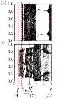
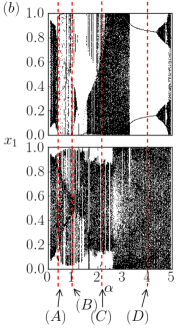
Figure 1: Bifurcation diagrams: (a) Bubbles ($R=1.0$); (b) Aerosols ($R=0.5$), without (top) and with (bottom) history force.In order to fit the diagram into the unit interval values of $2>x_{1}>1$ are plotted as $1-x_{1}$. The arrows point to the $\alpha$ values (A, B, C, D) chosen as case studies to illustrate the strong changes in the dynamics with inclusion of memory in Sec. IV.

III.2 Slow transient dynamics with memory

The basic difference in the transient behaviour with and without the history force is illustrated by a case of bubbles with 4 coexisting point attractors in the stroboscopic map. A detailed study of the dynamics will be given within case A of Sec. IV, here we concentrate only on the time needed to reach the attractor (depicted in Fig. 5a).

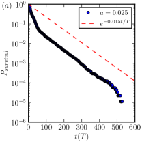
(a)

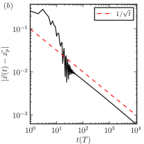
(b)

Figure 2: (a) Survival probability outside the four circles of radius $a=0.025$ around the attractor points as a function of time without history force obtained for an ensemble of particles. (b) The distance to the attractor as a function of time for a single particle initialized in the basin of attraction, with history force. The used parameters are $R=1.0$, $\alpha=0.5$, and time is measured in units of the period $T$ of the flow.

For the case without memory, it is numerically feasible to work with an ensemble of particles and to estimate the survival probabilities in a region outside the attractors. The particles are initialized homogeneously in space, and their positions are recorded at integer multiples of $T$. Around each attractor point (there are altogether 4 coexisting attractors) a circular disk of radius $a$ is prescribed and we determine the number of particles outside these disks. In Fig. 2a we see that the normalized number of particles staying outside the disks, the survival probability $P_{\text{survival}}$, decreases exponentially in time. This points to the existence of a chaotic saddle Lai and Tél (2011) which is discussed in more detail in Sec. IV. The particles outside the disk spend a long time on the chaotic saddle where they move upwards from one cell to the next. The escape rate from the chaotic saddle is found to be $\kappa=0.015/T$, out of which the average lifetime can be estimated via $1/\kappa$ as about $66T=132$ time units. This implies that the number of survivors decreases by a factor of $1000$ after $500T$ (Fig. 2a).

When taking into account the memory force, we also find four point attractors but they are reached extremely slowly. Due to the expensive calculation of the integral term up to $10^{4}$ periods, we have to restrict our calculation to the trajectory of a single particle. We initialize this particle within the basin of attraction of one of the attractors and monitor the distance $|\vec{x}(t)-\vec{x}_{p}|$ of this particle to the attractor point $\vec{x}_{p}$ in the stroboscopic map (Fig. 2b). We find that the long term behavior is not exponential, but rather a power law decay proportional to $t^{-1/2}$, as also observed in Daitche and Tél (2011). This diffusive behavior is a consequence of the history kernel in Eq. 1. The decay is obviously much slower than the one without memory. Here we chose the initial condition of the particle such that it does not rise but is trapped in the initial box. We see that even if trapping is immediate, the distance to the attractor decreases by only a factor of $10$ over the time interval of $500T$. Qualitatively, the existence of a periodic attractor can be explained by the observation that after a long time the trajectory is close to but not yet on the attractor, the memory of the early approach to the attractor decays, and the dynamics remembers only the motion in the close vicinity of the attractor, and a convergence becomes thus possible Daitche and Tél (2011). This mechanism also explains the long time needed for convergence. It is this slow power-law decay — coupled with the demanding numerical computations — that makes a precise numerical determination of all the attractors in the bifurcation diagram in the presence of the history force impossible. Due to this technical difficulty, in this work we shall follow trajectories or ensembles of trajectories for a sufficiently long time, plot the positions of the trajectories at this instant, and call this an (approximate) attractor.

III.3 Relative magnitude of the history force

As another general aspect, we see from the last term of Eq. 1 that the history force is proportional to ${A}^{1/2}$, therefore its influence is expected to be relatively more dominant for larger particles (smaller A). The ratio of the history $F_{h}(t)$ and the drag force $F_{St}(t)$ (at fixed densities) can be estimated from Eq. 1 as $A^{1/2}/A=A^{-1/2}$, although the exact value will also depend on the velocities of flow and particle, and their changes along the trajectory. In view of Eq. 6 this implies a proportionality to $\alpha^{1/3}$. This tendency is in harmony with simulation results presented in Fig. 3a and b, where the average ratio $\left<F_{h}(t)\left>/\right<F_{St}(t)\right>$ is plotted as a function of particle size $\alpha$. The deviations from the simple power law scaling are due to the fact that the integral in Eq. 6 and $v-u$ are not always of the same order in modulus. Note that the average of the history force can grow up to $80\%$ ($50\%$) of the Stokes drag for bubbles (aerosols). All this indicates that the history force must not be neglected.

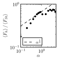
(a)

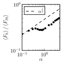
(b)

Figure 3: Average of the magnitude of the history force compared to the Stokes drag as a function of particle size, $\alpha$, for (a) $R=1.0$ and (b) $R=0.5$. For each parameter an ensemble of 10 random initial conditions in a cell are taken. The forces are measured and averaged over a time range of $500T$, and afterwards an ensemble average is also determined. The dashed lines represent a $\alpha^{1/3}$ curve, for comparison.

Although the dynamics for bubbles and aerosols are very distinct, the history force can produce similar effects in both cases. We illustrate this by analyzing in detail four specific cases, shown in Fig, 1.

IV Case studies

The cases are chosen in order to illustrate a fractalization of the basin boundaries and a deformation of the attractor (A), changes in transport characteristics (in trapping) (B), appearance of new attractors (C), and changes in the type of attractors (D). In the following subsections we will describe in detail each of these cases with one example for bubbles and one for aerosols.

IV.1 Fractalization of the basins of attraction, deformation of the attractors

We start our case study with very small particles ($\alpha=0.5$) where the effects of the history force are relatively mild. One can read of Fig. 3 that the history force corresponds here in magnitude to $\sim 50\%$ of the Stokes drag for bubbles and almost $30\%$ of the Stokes drag for aerosols. In both cases, bubbles and aerosols, we find four coexisting periodic, limit cycle attractors, each of which having their own basin of attraction, i.e. set of initial conditions that converge to that attractor. Although, the dynamics with and without history force appear to be very similar in this case, there are already clear differences. The most striking of them is that the basins of attraction change their topology. While the basin boundaries appear to be smooth without history force, they acquire a pronounced fractal character when the history force is included (see Fig. 4). These changes are of course consequences of changes in the particle dynamics. As a further illustration of this, we performed simulations with an ensemble containing a large number of particles ($N=10^{4}$). This particle ensemble is monitored over $120T$. A longer interval is not possible to choose due to the numerical cost of recording the history force with small time step for this number of particles.

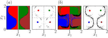
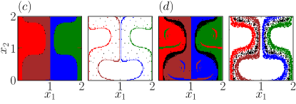
Figure 4: Comparisons of basins and attractors for $\alpha=0.5$ (a, c) without memory, (b, d) with memory, for (a, b) bubbles ($R=1.0$) and (c, d) aerosols ($R=0.5$). On the left and right of each panel are the basins of attraction and the four corresponding attractors (in red, blue, green and brown) obtained for $10^{4}$ particles at $t=120T$ in stroboscopic map in a double periodic representation. For better visibility we mark in the right figure of panel (a) the boxes (unit squares) within a cell. Points of the chaotic transients, that is particles which have not yet reached the attractors after $120T$, appear in black.

Bubbles are attracted to the vicinity of the vortex center, mainly because of the effect of the pressure force. Once there, they move on a closed periodic trajectory with the period $T$ of the flow. Therefore, in the double periodic representation in the stroboscopic map, these limit cycles appear as four point attractors: one in the neighborhood of the center of each box (Fig. 4a, b).

Aerosols, on the other hand, switch quasi-periodically from the vicinity of box centers to box boundaries, due to the time dependence of the flow, while moving from one cell to the next one downstream. In the process of sedimentation, they become confined horizontally to a region equivalent to one box size. We observe four quasiperiodic attractors. In a double periodic representation of the memoryless case they correspond to thin curves (Fig. 4c). In the presence of memory we find four color bands meandering about the vortices (Fig. 4d). The fattened appearance of these attractors is due to the presence of the long transients with power-law decay discussed in the previous section (Sec. IIIB).

Although the history force does modify the location and shape of the attractors for $\alpha=0.5$, their main character remains unchanged. One of such important characteristics for bubbles is the average rising height before becoming trapped by a vortex. The average rising speed of a particle close to the chaotic saddle is found to be $0.3$ box length per time unit without memory. Multiplying this with the average lifetime of $66T$, obtained in Sec. IIIB (see Fig. 2a), we find that bubbles typically rise $40$ length units (about $20$ cells) before becoming trapped. With memory, the great majority of initial conditions leads to a dynamics where particles get trapped by the vortices within the first $100T$. Although they take significantly longer times to reach the attractor within a single cell (see. Fig. 2b), the average trapping time to a single box is similar to the memoryless case.

In spite of similarities, there are, however, considerable local changes of the dynamics which we illustrate by plotting the attractors and the force vectors along pieces of them in a continuous time representation (Fig. 5). For bubbles, we see that the history force (in red) changes direction roughly with the change of the velocity of the flow. We illustrate this with the attractor in the left lower box of the cell (Fig. 5a) where we also mark the time instants $t=0,1/2,1,3/2$ along the limit cycles. The vectors of the history force change direction indeed at $t\sim 0$ and $t\sim 1$. When the particle is on the outer branch of the attractor, the vortex motion is counterclockwise, and pushes the bubble downwards. Along the inner branch (in the time interval $(1.12,1.88)$) the vortex is rotating clockwise and the fluid motion helps the rising of the bubble. The history force is seen to counteract the pressure force (in green). The resulting attractor is shifted further away from the vortex center then the one without memory.

For aerosols, the attractors contain regions of large curvatures which correspond to instants when the vortex rotations change sign. The history force drives particles on average away from the box center, and away from box boundaries when they eventually approach them. The trajectory contains a lower number of sharp curvatures, and the attractor is slightly shifted horizontally, as can be seen in Fig. 5b. The fact that the trajectories are more smooth implies that particles sediment slightly faster. In this particular example, the average vertical speed changes from $\sim-0.125$ box length per time unit without memory to $\sim-0.15$ box length per time unit with memory.

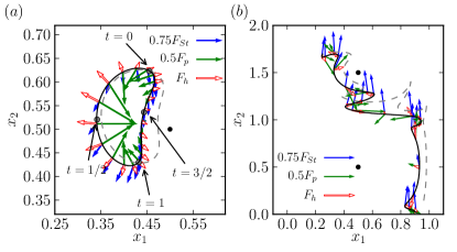
Figure 5: Force vectors along the attractor ($80T$ transients discarded) in a continuous-time planar representation. The history force and (for better visibility) three quarters of the Stokes drag and one half of the pressure force are shown at a few instances within a time interval of about $8T$. (a) $R=1.0$. Time instants corresponding to quarter periods are indicated along the limit cycle attractor. (b) $R=0.5$. The trajectory with history force is plotted over a shorter interval of about $6.5T$. In both panels black dots represent the center of a vortex and the dashed gray line is the attractor without the history force. Since the overall vertical difference is approximately the same in panel (b), the difference in times implies an increased sedimentation speed with memory.

IV.2 Vertical leaking

Next we investigate the behaviour of particles with $\alpha=1.0$. Their dynamics, without memory, consist of vertical motion until these particles get captured in one of four possible limit cycle attractors (Fig. 6a and b), for both bubbles and aerosols. For bubbles, the attractors are periodic with period $T$. Aerosols have more complicated limit cycles of period $12T$. In the presence of the history force, we observe that particles cannot get trapped vertically and move along extended quasiperiodic attractors (Fig. 6c and d). Hence, the history force leads to vertical leaking in this case. The history force is strong enough to essentially modify the original periodic attractors into quasiperiodic ones. Bubbles are observed to converge to two symmetric quasiperiodic attractors, while for aerosols the number of attractors remains four (they appear in symmetric pairs). In this latter case, the sedimentation velocities on the different attractors do not differ. What changes is the time to reach the attractor for different initial conditions (this is reflected by the different locations of the two pairs of attractor pieces plotted after the same time in Fig. 6d). The rising velocity of the bubble (Fig. 6c) is found to be $\sim 0.31$ box length/ time unit. The sedimentation velocity of the aerosols with memory is $\sim-0.33$ box length / time unit (Fig. 6d).

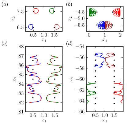
Figure 6: Comparison of attractors pieces for $\alpha=1$ in continuous time in the planar representation (trajectories are followed over a period of $20T$, after discarding transients of length $80T$). (a) bubble and (b) aerosol dynamics without history force. (c) bubble and (d) aerosol dynamics with memory effects. The black dots represent the center of vortices.

In summary, the effects of the history force in the case of $\alpha=1$ are that trapping is no longer possible, and the attractors change from periodic to quasiperiodic, and vertical leaking occur. Additionally, the number of attractors changes for bubbles.

IV.3 Appearance of new attractors, and horizontal localization

We illustrate that new types of attractors appear due to memory effects for aerosols and bubbles of size $\alpha\sim 2$. A related feature is that the history force prevents the particles to cross the vertical boundaries of the cell. This confinement of the dynamics breaks off the horizontal diffusion present without memory (Fig. 7), and results in the emergence of new types of attractors in the system.

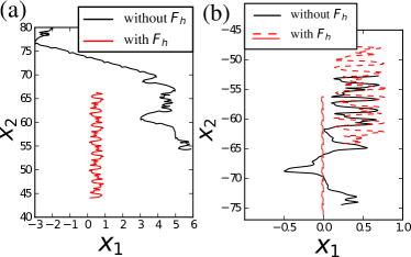
Figure 7: Continuous time trajectories over $10T$ for (a) bubbles and (b) aerosols. In both simulations a transient of $50T$ is discarded. Without memory a trajectory on the chaotic attractor is shown in (a) which strongly spreads horizontally. With memory a confined periodic attractor is traced out (the red attractor of Fig. 8c). In (b) part of one of the chaotic attractors is shown without memory (the red attractor in Fig. 9b, which communicates with its neighboring cell. With memory we display two of the six quasi periodic attractors (I’ and II’ of Fig. 9d)

For bubbles ($R=1$) we find chaotic behaviour without memory with a single symmetric attractor, as shown in a double periodic stroboscopic representation in Fig. 8a. It crosses the cell walls, i.e., the movement while rising is not confined neither horizontally nor vertically. In the horizontal motion of bubbles we find that there are two perceived time scales: A fast local movement, and a slow cell-to-cell horizontal diffusion. We can describe this as an intermittent horizontal spreading of trajectories (Fig. 7a).

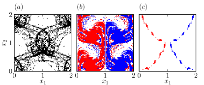
Figure 8: Comparison of attractors and basins for bubbles with $\alpha=2,R=1$. (a) Single chaotic attractor without history force. (b) Basins (white points represent initial conditions which have not reached the attractor in $120T$) and (c) two attractors for the dynamics with memory effects. All plots are obtained from the advection of $10^{4}$ particles at $t=120T$ in the stroboscopic map.

The inclusion of the history force has a very clear effect: It confines the trajectories in the horizontal direction. This leads to the appearance of two quasiperiodic attractors (Fig. 8c) instead of a single chaotic one (red curve in Fig. 7a).

The memoryless aerosol dynamics ($R=0.5$) in this parameter range exhibits two chaotic attractors, which are bounded in configuration space to the middle or to the two vertical edges of the cell, respectively (Fig. 9b). The trajectories cross the vertical box borders implying that sedimenting particles spread horizontally, but not further then the next neighbor from which their return. In the presence of the history force, the particles are no longer able to cross the vertical cell borders, the motion becomes localized horizontally to a single box width (Fig. 9d). In addition, instead of two (Fig. 9b), six attractors appear in 3 symmetric pairs, denoted by I, I’ and II in Fig. 9d. These attractors are no longer chaotic, they exhibit quasi-periodic behaviour. One pair of the attractors (II) meanders across the box, and the others (I, I’) wiggle very close to the box borders in the stroboscopic map, although they never cross the lines $x_{1}=0$ or $1$ or $2$ (I and II in Fig. 9; note the strong horizontal magnification in I of the region near the box division). In (I) we see, when plotting the force vectors again, that all point practically in the vertical direction, and therefore there is no tendency for a border crossing due to inertia. Note that there is a cusp in the attractor indicating a sign change in the rotational direction of the vortices. In (II), the history force points basically towards the vortex centers, helping to confine the trajectories to a single box horizontally. The basins of attraction have fractal boundaries both with and without memory (Fig. 9a and c).

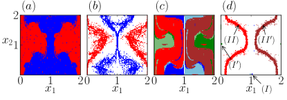
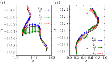
Figure 9: Comparison for aerosols with $\alpha=2.2$. (a), (b): attractor structure without memory, basins (a) and attractors (b). The two chaotic attractors are marked by red and blue. (c), (d): attractor structure with memory, six attractors are present. The attractors are obtained from the advection of $10^{4}$ aerosol particles ($R=0.5$) at $t=120T$. (I), (II): trajectories on attractors I and II (plotted over $1.6T$, after discarding transients of $40T$) with the corresponding force vectors.

IV.4 Changes in the nature of the attractor

In the previous examples we already observed changes in the type of attractor from periodic to quasiperiodic due to the impact of the history force. Besides this transition, we find others which we discuss here with an example of a conversion from periodic to chaotic dynamics, and vice versa. The first occurs for large aerosols, and the second for large bubbles. In both situations the magnitude of the history force is very strong, corresponding to $\sim 80\%$ (bubbles) and $\sim 35\%$ (aerosols) of the Stokes drag (see Fig. 3). As previously, there are strong changes of the horizontal diffusivity of the advected particles. In the two examples the periodic attractors are characterized by high diffusivity, where particles move almost diagonally across the cells (Fig. 10). We characterise diffusivity by the variance of the displacements within a particle ensemble. Since periodic attractors appear in symmetric pairs, this quantity remains well defined in these cases. The chaotic attractors, on the other hand, have trajectories with comparatively lower horizontal diffusion (Fig. 10). Here we again observe a change in the number of attractors: We have a single one for the chaotic and two symmetric ones for the periodic dynamics.

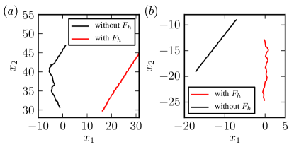
Figure 10: (a) Trajectories of bubbles $R=1$, $\alpha=5.0$ over $30T$ on the attractor after $16T$ transients, in continues time representation. In the presence of history only one of the attractors is represented; (b) trajectories of aerosols $R=0.5$, $\alpha=4.0$ on the attractor over $10T$ after $10T$ transients, in continuous time representation. In the memoryless case only one of the attractors is represented.

IV.4.1 From chaotic to periodic

The transition from a single chaotic attractor into two periodic ones we exemplify with a case found for large bubbles $\alpha=5.0$. The dynamics without memory effects is chaotic: The trajectories diffuse slowly horizontally from one cell to the next. The single attractor in a double periodic representation shows a pronounced fractal structure, Fig. 11a. When the memory is included we see two periodic attractors of period $2T$, which can be seen as two period-2 orbits in the double periodic representation of Fig. 11c. The boundary of the basins of attraction for these periodic attractors is of riddled type  Lai and Tél (2011); Alexander et al. (1992), that is the fractal dimension is nearly $2$ (Fig. 11b). As a consequence the transient times to reach the attractors are very long ($\gg 100T$).

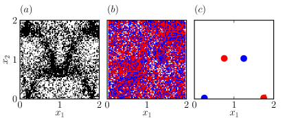
Figure 11: Comparison for bubbles of $\alpha=5,R=1$. (a) Single chaotic attractor without memory. (b) The basins of attraction and (c) two period-2 attractors with memory. All plots are obtained from the advection of $10^{4}$ bubbles at $t=120T$. White points in (b) represent initial conditions which have not reached the attractor in the given time interval.

These periodic attractors, in a continuous time representation, cross the cell almost diagonally (Fig. 12c). The inclusion of the history increases the diffusivity in the system, since the horizontal crossing of the box boundaries is facilitated. To capture this effect we compute the horizontal component of all the forces acting on the advected particle along the trajectory as a function of $x_{1}$. In case of chaotic dynamics we work with average values of forces felt by a single particle on the attractor in the double periodic representation over a time of $500T$. For the periodic case we just plot the horizontal component of the forces as a function of $x_{1}$. (We consider forces as positive if they are directed from left to right.) We observe that at the box boundaries among the horizontal component of all the forces the history force provides the largest contribution, pulling the particle from one box to the next (Fig. 12a). This results in an enhanced horizontal diffusivity.

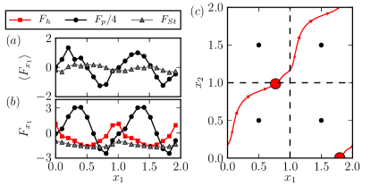
Figure 12: Bubble dynamics for $\alpha=5,R=1$. Horizontal component of the forces at different positions $x_{1}$ computed along particle trajectory: (a) average forces on the chaotic attractor without memory; (b) forces on the attractor of panel (c). (c) Continuous time trajectory of the red attractor of Fig. 11c. Large red dots correspond to the positions of the attractor in the Poincare map. The centers of four vortices are represented as black dots.

IV.4.2 From periodic to chaotic

We illustrate the transition from periodic to chaotic with a case of large aerosols, $\alpha=4.0$. Without history force, we observe cell crossing periodic trajectories spreading widely in the horizontal direction (Fig. 10b). The system exhibits two periodic attractors of period $2T$, and basins of attraction with fractal boundaries (Fig. 13a). When the history force is included the two periodic attractors change into one chaotic attractor (see Fig. 13b and c). The action of the history force is opposite compared to the previous example: it weakens the strength of horizontal diffusion.

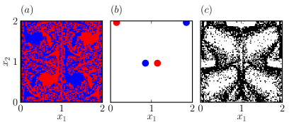
Figure 13: Comparison for aerosols of $\alpha=4,R=0.5$. The basins of attraction (a) and the corresponding periodic attractors (b) without memory. The chaotic attractor (c) in the presence of the history force. All plots determined from the advection of $10^{4}$ aerosol particles at $t=120T$.

To better understand the spreading behaviour we determine the horizontal components of the three forces as a function of coordinate $x_{1}$. We use, as previously, mean values over $500T$ for the dynamics on the chaotic attractor. We observe that without memory, not only the pressure force controls the horizontal movement, but also the Stokes drag (see Fig. 14a). The graph of the pressure force is asymmetric and the positive part dominates, the Stokes drag has permanently negative sign. (The signs of the forces are the opposite on the symmetric counterpart of this attractor.) When the memory is included, we observe a complete change of the horizontal components of the forces (see Fig. 14b); the forces have no longer a preferential direction, and decrease in magnitude. The horizontal components of the three forces provide a kind of string force pointing towards the cell center. In the presence of the history force the positive and negative contributions of the horizontal forces nearly balance each other. As a consequence it is easier for the trajectories to turn, which results in an increase of the curvature. The motion withing a cell is followed also in this case by a cell-to-cell horizontal displacement. We can describe this again as an intermittent horizontal spreading of trajectories (Fig. 13c).

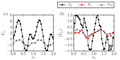
Figure 14: Horizontal component of the forces acting on an aerosol particle as a function of $x_{1}$: (a) computed for the blue attractor without history force (Fig. 13b); (b) with history force. Here, as the trajectory is chaotic, we plot a temporal average over $500T$.

Having described the main effects of the history force on the attractors of the system, we now move to the effect on the transport properties of the flow.

V Transport properties

V.1 Horizontal spreading

Here we compare the transport properties in the horizontal direction with and without the history force. We observe that the history force can introduce strong changes in the horizontal dynamics: in a wide range of parameters, for both aerosols and bubbles, the effect of memory results in weakening or even blocking the spreading. To quantify this effect, we determine the horizontal displacements $x_{1,t}$ from the initial position for $N=30$ trajectories after a fixed time interval $t=140T$. The initial conditions are randomly chosen within a cell. We evaluate the mean $\left<x_{t}\right>$ and the variance

$$\mbox{var}(x)=\left(\left<x^{2}_{t}\right>-\left<x_{t}\right>^{2}\right)^{1/2}$$ (13)

over the ensemble. The results for the variance are plotted in Fig. 15a and b. We note that the computational demands do not allow us to evaluate the variance over longer time intervals (and larger ensembles) from which diffusion coefficients could be determined with some confidence. In addition, the intermittent behavior mentioned earlier between staying within a cell and cross-cell horizontal motion makes us believe that in some cases the spreading is superdiffusive. With these constraints we characterize horizontal diffusivity in terms of the variance. Note that because of using several initial conditions, the behavior over all attractors is averaged.

As a function of the size parameter, we can distinguish three regimes in Fig. 15a and b. Particles of small sizes stay bound to the cell where they are initiated, and the variance is below unity. This region is marked as “confined”. For larger particles, we see a tendency of increase (beyond unity) in the variance due to spreading into the neighboring cells. The strength of spreading increases with the particle size. This interval of $\alpha$ is called “diffusive”. For even larger particles the movement on the attractors turns into a ballistic-like motion where particle cross the cells almost diagonally. This periodic motion corresponds to the approximately horizontal plateaus in Fig. 15, which we call “periodic”.

With the history force, the horizontal confinement to the original cell persists through a wider range of sizes. Diffusion appears at about $\alpha=2.8$ for bubbles and at about $\alpha=3.5$ for aerosols, Fig. 15. This horizontal confinement up to $\alpha=2.8$ is in harmony with the lower panels of the bifurcation diagrams of Fig. 1. In the interval $2.8<\alpha<3.5$ for aerosols the stretching of the bifurcation diagram over the unit interval only implies a communication between neighbouring cells without further spreading.

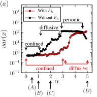
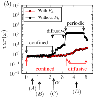
Figure 15: Variance of horizontal displacement with and without memory, evaluated at $t=140T$. $\alpha$ values corresponding to cases treated in Sec. III.1 are marked by labels $A,\dots,D$

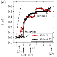
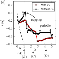
Figure 16: Comparison of average vertical velocities $\left<v_{2}\right>$ with and without memory. (a): Bubbles, $R=1.0$; (b): Aerosols, $R=0.5$. The $\alpha$ values corresponding to cases treated in Sec. III.1 are marked by labels $A,\dots,D$. The settling/ raising velocities in a fluid at rest are plotted with dashed lines.

V.2 Vertical velocity

Another important feature is transport in the vertical direction. A useful quantity for characterizing its strength is the average vertical velocity, obtained again over an ensemble of trajectories. The average values are computed for 30 randomly initiated trajectories within a cell over $50T$ after cancelling $50T$ transients. This quantity is also affected by the history force, the most striking effect being the disappearance of vertical trapping ($\left<v_{2}\right>=0$) for aerosols of any size (see Fig. 16b). For bubbles the history force reduces the range of trapping, which is only possible for very small bubbles, up to $\alpha=0.4$ (in a size parameter range about $2$ times smaller than without memory), as can be seen in Fig. 16a The action of the forces, in the given flow, determines the shape of the attractors in a given phase instance. The average velocity on the attractors depends on their shape, and this might result e.g. in lower velocities when larger portions of the attractor are close to vortex centers where the flow is weak. This explains the larger sinking velocities in the presence of memory for $\alpha>3$ than those without. Periodic trajectories belong again to the plateaus of velocities. It is interesting to compare these results with those valid in a fluid at rest. The dimensionless vertical velocity is given then by Eqs. 4 and 5. In view of Eq. 7, and the fact that $w_{1}=1.6$ we find for our bubbles and aerosols that $W=\pm 0.8\alpha^{2/3}$. These curves are plotted as dashed lines in Fig 16, they correspond to much larger velocities than the measured ones. This difference shows how important the effect of the flow is on the vertical motion, $W$ cannot even be used as an estimate.

VI Conclusion

We compared the dynamics of chaotic advection of the finite size particles using the full Maxey-Riley equations with the well spread approximation which ignores the history force term. We observed strong differences between both dynamics, such as a large increase in the transient time, and a modification of the nature and number of attractors. Directly from the equations, one can see that the effect of the history force increases with the particle size. For small particles, the history force is relatively weak compared to other forces, it is, however, already large enough to affect the shape and the position of the attractors in configuration space, and in particular it causes the basins of attraction to acquire fractal boundaries. For slightly larger particles, for which particle trapping in a single box is possible in the memoryless case, the history force generates vertical leaking so that the resulting trajectories jump from one cell to the next in the vertical. The fact that trapping fully disappears for aerosols, and becomes restricted to very small bubbles only, is one of the most striking effects of memory. This might be associated with a decrease in the number of attractors. With a further increase of the size parameter, the history force strongly decreases the horizontal spreading of particles, it might even prevent the attractors to cross from one box to the next in the horizontal. This weakening in horizontal spreading can go along with an increases in the number of attractors. We also find that the effect of history can be the opposite: in such cases the history force pulls the particles to the next box, resulting in a change in the type of attractor from chaotic to periodic. This might be the dynamical background of the changes found in the transport properties of the system.

Based on the strong differences found with the inclusion of memory effects, we argue that it is essential to consider the Maxey-Riley equations in their full form, in order to account for the full complexity of advection dynamics.

The impact of the history force on transport properties of inertial particles in flows may have significant implications for sedimenting particles in the ocean. Vertical export of marine aggregates is considered to be one important process to export carbon into deeper ocean layers De La Rocha and Passow (2007). Here often settling velocities (Eq. 4) are used to estimate fluxes of particles. However, our results show, that these settling velocities (dashed line in Fig. 16) turn out to be much faster than the ones obtained from moving inertial particle in a flow. Therefore, export rates of aggregates based on settling velocities in still fluids appear to be dramatically overestimated compared to the ones which take the motion in a fluid flow explicitly into account.

VII Acknowledgment

We would like to thank A. Daitche for valuable discussions. We acknowledge support from COST-Action MP0806 “Particles in Turbulence”. U.F. would like to thank R. Roy and his group for their hospitality and acknowledges support from the “Burgers Program for Fluid Dynamics” of the University of Maryland at College Park. T.T. acknowledges the support of OTKA grant NK100296 and of the Alexander von Humboldt Foundation.

References

- Cartwright et al (2010) J. H. E. Cartwright et al, in Nonlinear Dynamics and Chaos: Advances and Perspectives, Understanding Complex Systems, edited by M. T. et al (Springer Berlin Heidelberg, 2010) pp. 51–87.
- Nishikawa et al. (2001) T. Nishikawa, Z. Toroczkai, and C. Grebogi, Physical Review letters 87, 038301 (2001).
- Nishikawa et al. (2002) T. Nishikawa, Z. Toroczkai, C. Grebogi, and T. Tél, Physical Review E 65, 026216 (2002).
- Zahnow et al. (2008) J. C. Zahnow, R. D. Vilela, U. Feudel, and T. Tél, Physical Review E 77, 055301 (2008).
- Bec (2003) J. Bec, Physics of Fluids 15, L81 (2003).
- Zahnow and Feudel (2009) J. C. Zahnow and U. Feudel, Nonlin. Processes Geophys. 16, 677 (2009).
- Calzavarini et al. (2008) E. Calzavarini, M. Cencini, D. Lohse, and F. Toschi, Physical Review Letters 101, 084504 (2008).
- Bec et al. (2005) J. Bec, A. Celani, M. Cencini, and S. Musacchio, Physics of Fluids 17, 073301 (2005).
- Fiabane et al. (2012) L. Fiabane, R. Zimmermann, R. Volk, J.-F. Pinton, and M. Bourgoin, Physical Review E 86, 035301 (2012).
- Gibert et al. (2012) M. Gibert, H. Xu, and E. Bodenschatz, J. Fluid Mech. 698, 160 (2012).
- Falkovich et al. (2002) G. Falkovich, A. Fouxon, and M. G. Stepanov, Nature 419, 151 (2002).
- Drótos and Tél (2011) G. Drótos and T. Tél, Physical Review. E 83, 056203 (2011).
- Wilkinson et al. (2008) M. Wilkinson, B. Mehlig, and V. Uski, Astrophys. J. Suppl. 176, 484 (2008).
- Benczik et al. (2002) I. J. Benczik, Z. Toroczkai, and T. Tél, Physical Review Letters 89, 164501 (2002).
- Tél et al. (2005) T. Tél, A. de Moura, C. Grebogi, and G. Károlyi, Physics Reports 413, 91 (2005).
- Daewel et al. (2011) U. Daewel, C. Schrum, and A. Temming, Fisheries Oceanography 20, 479–496 (2011).
- Zhang and Li (2003) J.-J. Zhang and X.-Y. Li, AIChE Journal 49, 1870 (2003).
- Crowe et al. (1998) C. C. T. Crowe, M. Sommerfeld, and Y. Tsuji, Multiphase Flows with Droplets and Particles Flows (CRC Press, Boca Raton, 1998).
- Michaelides (2006) E. E. Michaelides, Particles, Bubbles and Drops: Their Motion, Heat And Mass Transfer (Word Scientific, Singapore, 2006).
- Logan (2012) B. E. Logan, Environmental transport processes (Wiley, Hoboken, N.J., 2012).
- Zahnow et al (2009) J. C. Zahnow et al, Physical Review E 80, 026311 (2009).
- Zahnow et al. (2011) J. C. Zahnow, J. Maerz, and U. Feudel, Physica D 240, 882 (2011).
- Maxey and Riley (1983) M. R. Maxey and J. J. Riley, Physics of Fluids 26, 883 (1983).
- Auton et al. (1988) T. R. Auton, J. C. R. Hunt, and M. Prud’Homme, J. Fluid Mech. 197, 241 (1988).
- Basset (1888) A. B. Basset, A Treatise on Hydrodynamics (Bell, Cambridge, 1888).
- Mordant and Pinton (2000) N. Mordant and J.-F. Pinton, The European Physical Journal B 18, 343 (2000).
- Candelier et al. (2004) F. Candelier, J. R. Angilella, and M. Souhar, Phys. of Fluids 16, 1765 (2004).
- Daitche and Tél (2011) A. Daitche and T. Tél, Physical Review Letters 107, 244501 (2011).
- van Hinsberg et al. (2011) M. van Hinsberg, J. ten Thije Boonkkamp, and H. Clercx, J. Comput. Phys. 230, 1465 (2011).
- Vojir and Michaelides (1994) D. Vojir and E. Michaelides, Int. J. Multiphase Flow 20, 547 (1994).
- Daitche (2012) A. Daitche, arXiv:1210.2576 (2012).
- Toegel et al. (2006) R. Toegel, S. Luther, and D. Lohse, Physical Review Letters 96, 114301 (2006).
- Garbin et al (2009) V. Garbin et al, Physics of Fluids 21, 092003 (2009).
- Chandrasekhar (1961) S. Chandrasekhar, Hidrodynamics and Hidromagnetic Stability (Dover, Dover, 1961).
- Maxey (1987) M. R. Maxey, Phys. Fluids 30, 1915 (1987).
- Zahnow and Feudel (2008) J. C. Zahnow and U. Feudel, Physical Review E 77, 026215 (2008).
- Simon et al. (2002) M. Simon, H. P. Grossart, B. Schweitzer, and H. Ploug, Aquatic Microbial Ecology 28, 175 (2002).
- Mann and Lazier (2005) K. Mann and J. Lazier, Dynamics of Marine Ecosystems: Biological-Physical Interactions in the Oceans, 3rd ed. (Wiley, Blackwell, 2005).
- De La Rocha and Passow (2007) C. L. De La Rocha and U. Passow, Deep Sea Research II 54, 639 (2007).
- Riley et al (2012) J. S. Riley et al, Global Biogeochemical Cycles 26, GB1026 (2012).
- Bartholomä et al. (2009) A. Bartholomä, A. Kubicki, T. H. Badewien, and B. W. Flemming, Ocean Dynamics 59, 213 (2009).
- Oakey and Elliott (1982) N. S. Oakey and J. A. Elliott, J. Phys. Oceanography 12, 171 (1982).
- Lai and Tél (2011) Y.-C. Lai and T. Tél, Transient chaos: complex dynamics on finite-time scales (Springer, New York, 2011).
- Alexander et al. (1992) J. Alexander, J. A. Yorke, Z. You, and I. Kan, Int. J. Bif. Chaos 02, 795 (1992).