Electronic structure and transport in graphene: quasi-relativistic Dirac – Hartry – Fock self-consistent field approximation

H. V. Grushevskaya and G. G. Krylov
E-mail: grushevskaja@bsu.by
Physics Department, Belarusian State University, 4 Nezalezhnasti Ave., 220030 Minsk, BELARUS

1 Introduction

Graphene and graphene-like materials are considered today as a prominent candidates to be used in new devices with functionality based on quantum effects and(or) spin-dependent phenomena in low-dimensional systems. Technically, the main obstacle to such devices implementation is the lack of methods that provide minimizatioon of distortion of these material unique properties in bulk nanoheterostructures. Theoretical approaches and computer simulation play an important role in systematic search of this kind of nanostructures for nanoelectronic applications.

However, significant part of all theoretical consideration of graphene-like materials as well as modern model representations of charge transport in these systems on pseudo-Dirac massless fermion model, originally based on tight binding approximation and applied to the description of graphite [1, 2, 3, 4], which is a bulk material.

According to this approach [2], $\pi_{z}$-electrons in graphene are massless fermion type quasiparticle excitations moving with the Fermi velocity. The approach has been seriously developed and successfully applied to a number of experimental situation, some related review papers on the topics and further references are in [17, 18]. There are few known key points where (at our knowledge) one could expect the necessity of some generalized consideration. The first one is the cyclotron mass dependence upon the carriers concentration. Due to weakness of the signal, modern experimental techniques can register cyclotron mass of charge carriers which is just a little smaller than 0.02 of a free electron mass [5, 6, 7, 8]. Assessments are absent whether this mechanism of conductivity prevails in the region of very small values of charge carriers concentration.

The another point is the experimentally observable carrier asymmetry in graphene. According to modern theoretical concepts the bands for pseudo-relativistic electrons and holes in graphene must be symmetrical. With this in mind in the paper [9] in the generalized gradient approximation there were modelled the hexagonal Si and Ge, with the same structure as in graphene. But the electrons and holes bands near the Dirac points $K$ in the Brillouin zone turned out to be strongly asymmetric ones for both cases. Firstly, a Dirac cone deformation takes place far away from a circular shape, as for the second, the Dirac velocities for the valent and conduction bands are different [9]. Therefore, one can assume the existence of some asymmetry in the behavior of pseudo-relativistic electrons and holes of the graphene as well. Since the value of the asymmetry seems to be very small, for its experimental observation one should use a highly sensitive method, such e.g., as based on the measurement of noises [10]. For graphene, such a method is based on large amplitudes of non-universal fluctuations of charge carriers current in the form of nonmonotonic $1/f$ noise in the crossover region of the scattering [11]. At high charge densities, the contribution to the resistance of clean graphene basically gives the scattering of charge carriers on long-range impurities at ordinary (symplectic) diffusion. Regime of pseudo-diffusion with a charge carriers scattering on short-range impurities is realized in the vicinity of the Dirac points of the Brillouin zone. In the papers [12, 13] measurements of quantum interference noise in a crossover between a pseudodiffusive and symplectic regime and magnetoresistance measurements in graphene p-n junctions have been performed, which established asymmetric behaviour of pseudo-relativistic electrons and holes based on asymmetric form of non-monotonic dependence of noise and magnetoresistance. And the third known key point needed theoretical explanation is the replicas existence. A weakly interacting epitaxial graphene on the surface of Ir(111) has a non-distorted hexagonal symmetry due to the weakness of the interaction with the substrate in temperature range up to a room temperature. Therefore in ARPES (angle-resolved photo-electron spectroscopy) spectra, the perturbation of the band structure is manifested in the form of replica of the inverted Dirac cone and mini-gaps in places of quasi-crossings of replicas and the Dirac cone [14]. Authors of paper [14] propose replicas existence explanation such that replicas are produced only in the areas of convergence of C and Ir atoms, that explains the weak intensity of photoelectron emission replicas and brightness of the main cone. However, besides different intensity, the asymmetry of photoelectron emission spectra also manifests itself in the fact that maxima from the replicas are below then zero maximum ($E-E_{F}\approx 0$) of Dirac cone in the ARPES spectrum at the same angle of incidence of photons and with are equal to maxima of ARPES spectrum of replicas oppositely arranged on the hexagon. And conversely, if the corners of oppositely disposed replicas are in the neighborhood $E-E_{F}\approx 0$, the Dirac cone in the ARPES spectrum is located lower. The above described is possible if axes of the Dirac cone and its replicas are not parallel. It means that the top of the replica does not correspond to the corners of the hexagonal mini Brillouin zone, centered at the Dirac cone corner for the epitaxial graphene on the surface of Ir(111). It has been also demonstrated that epitaxial graphene on SiC(0001) holds a hexagonal mini Brillouin zone near the Dirac points [15, 16].

And at last, a bit more philosophical but also important comment. The majority of modern software for ab initio band structure simulations uses models being some variant of the Dirac equation or at least take into account the known relativistic corrections to the Schrödinger equation when attacking the problems. The quasi-Dirac massless fermion approach based purely on tight binding non-relativistic Hamiltonian seems to be oversimplified and hardly extendable.

With the goal to investigate the balance of exchange and correlation interactions the ab initio band structure simulations of loosely-packed solids(it was used the developed generalization of the LMTO method) have been performed and demonstrated that the strong exchange leads to appearance of an energy gap in the spectrum whereas strong correlation interactions leads to tightening of this gap [20]. The spin-unpolarized ab initio simulations of partial electron densities of two-dimensional graphite have shown that the material is a semiconductor. Interlayer correlations tighten the energy gap that results in semi-metal behaviour of three-dimensional graphite [20]. This means that in the absence of correlation holes, the correlation interaction in a monoatomic carbon layer (monolayer) is weak in comparison with the exchange. This theoretical prediction for spin-nonpolarized graphene were confirmed experimentally in [15, 16], where it was demonstrated a bandgap in bilayer graphene on SiC(0001) and its diminishing up to vanishing in multilayer graphene.

By the way, in a monolayer graphene on SiC(0001) one observes the dispersion of the Dirac cone apexes [15, 16].

Experimentally manufactured quasi-two-dimensional systems, such as graphene, carbon armchair nanotubes and ribbons as well as some types of zigzag carbon nanotubes manifest metallic properties (see, for example, [17, 19]). In this regard, there are discrepancies between theoretical predictions and experimental data.

Therefore, based on the results of ab initio spin-unpolarized simulations of two-dimensional and three-dimensional graphite [20], we can make the following assumption. Carbon low-dimensional systems having the properties similar to graphite-like materials should possess spin-polarized electronic states with the correlation holes (a magnetic ordering). Enhancing of correlation interaction due to correlation-hole contribution leads to tightening of the energy gap and, as a consequence, the emergence of semi-metal conductivity.

The approach we use has been developed earlier in [22] and applied for graphene-like material in [23].

The goal of this chapter is to represent a Dirac – Hartree – Fock self-consistent field quasirelativistic approximation for quasi-two-dimensional systems and to describe the origin of asymmetry of electron – correlation hole carriers in graphene-like materials.

2 Graphene model bands with correlation holes

Single atomic layer of carbon atoms (two-dimensional graphite) is called monolayer graphene. Its hexagonal structure can be represented by two triangular sublattices A, B [21]. The primitive unit cell of the graphene contains two carbon atoms C_A and C_B belonging to the sublattices A and B respectively.

The carbon atom has four valent electrons s, p_x, p_y, p_z. Electrons s, p_x, p_y are hybridized in the plane of the monolayer, p_z-electron orbitals form a half filled band of $\pi$-electron orbitals on a hexagonal lattice.

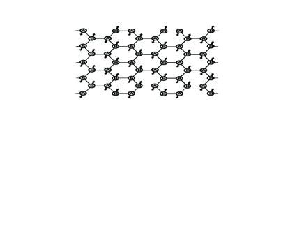
Let electrons with spin $+\sigma$ ”down”  (”up”) are placed on the sublattice $A\ (B)$, and the electrons with spin $-\sigma$ ”up”  (”down”) – on the sublattice $B\ (A)$, as shown in Fig. 1.

Figure 1: Hexagonal lattice of carbon monolayer with spin ordering sublattices $A,\ B$.

With such a symmetry of the problem, all the relevant bands of sublattices are half-filled and are formed due to correlation holes. In the representation of secondary quantization and Hartree – Fock self-consistent field approximation, when not accounting for the electron density fluctuation correlation, the hole energy $\epsilon(k)$ is simply added to the electron energy $\epsilon_{m}(0)$ [30]:

$$\left[H(\vec{r})+\hat{V}^{sc}(kr)-\hat{\Sigma}^{x}(kr)\right]\psi_{m}(kr)=\left(\epsilon_{m}(0)-\sum_{j=1}^{n}\hat{\epsilon}^{\dagger}P_{j}\right)\psi_{m}(kr),$$ (1)

$$\hat{\epsilon}^{\dagger}=\epsilon(k)\hat{I}$$ (2)

because the sum $\sum_{j}P_{j}$ of projection operators $P_{j}$ in in parentheses equals to the identity operator $\hat{I}$: $\sum_{j}P_{j}=\hat{I}$.

We denote spinor wave functions of the valent electrons of graphene as $\widehat{\chi^{\dagger}_{\sigma}}(\vec{r}_{A})\left|0,+\sigma\right>$ and $\widehat{\chi^{\dagger}_{-\sigma}}(\vec{r}_{B})\left|0,-\sigma\right>$. From Fig. 1 it follows that the spinor quantum fields $\widehat{\chi^{\dagger}_{\sigma}}(\vec{r}_{A})$ and $\widehat{\chi^{\dagger}_{-\sigma}}(\vec{r}_{B})$ are transformed into each other under the mirror reflection $A\to B$. Therefore, a quasi-particle excitation in the proposed model of graphene is a pair of an electron and a correlation hole. As an electron-hole pairs at the same time represent themselves their proper antiparticle, the wave functions belong to the space of Majorana bispinors $\Psi^{\prime}$, and upper and lower spin components $\psi^{\prime}$, $\dot{\psi}^{\prime}$ are transformed via different representations of the Lorenz group

$$\Psi^{\prime}=\left(\begin{array}[]{c}\psi^{\prime}_{\sigma}\\[0.28453pt] \dot{\psi}^{\prime}_{-\sigma}\end{array}\right)=\left(\begin{array}[]{c}e^{{\kappa\over 2}\vec{\sigma}\cdot\vec{n}}\psi_{\sigma}\\[0.28453pt] e^{{\kappa\over 2}(-\vec{\sigma})\cdot\vec{n}}\dot{\psi}_{-\sigma}\end{array}\right).$$ (7)

It means that $\widehat{\chi^{\dagger}_{\sigma}}(\vec{r}_{A})\left|0,+\sigma\right>$ behaves as a component $\psi_{\sigma}$, and $\widehat{\chi^{\dagger}_{-\sigma}}(\vec{r}_{B})\left|0,-\sigma\right>$ – as a component $\dot{\psi}_{-\sigma}$ of bispinor (7). Using the expression (7) and properties of these operators:

$$\widehat{\chi^{\dagger}_{-\sigma_{{}_{A}}}}(\vec{r})\left|0,+\sigma\right>\stackrel{{\scriptstyle def}}{{=\!=}}0,\ \widehat{\chi^{\dagger}_{+\sigma_{{}_{B}}}}(\vec{r})\left|0,-\sigma\right>\stackrel{{\scriptstyle def}}{{=\!=}}0$$

one gets the following expression for the bispinor wave function $\left|\Psi\right>$ of an electron in graphene:

$$\left|\Psi\right>=\left(\begin{array}[]{c}\widehat{\tilde{\chi}^{\dagger}_{-\sigma_{{}_{A}}}}(\vec{r})\left|0,-\sigma\right>\\[1.70717pt] \widehat{\tilde{\chi}^{\dagger}_{\sigma_{{}_{B}}}}(\vec{r})\left|0,+\sigma\right>\end{array}\right)=\left(\begin{array}[]{c}\left|0,+\sigma\right>\widehat{\chi^{\dagger}_{-\sigma_{{}_{A}}}}(\vec{r})\left|0,-\sigma\right>\\[1.70717pt] \left|0,-\sigma\right>\widehat{\chi^{\dagger}_{\sigma_{{}_{B}}}}(\vec{r})\left|0,+\sigma\right>\end{array}\right)$$ (12)

$$=\left(\begin{array}[]{c}\left|0,+\sigma\right>\widehat{\chi^{\dagger}_{-\sigma_{{}_{A}}}}(\vec{r})\left|0,-\sigma\right>+\left|0,-\sigma\right>\widehat{\chi^{\dagger}_{-\sigma_{{}_{A}}}}(\vec{r})\left|0,+\sigma\right>\\[1.70717pt] \left|0,-\sigma\right>\widehat{\chi^{\dagger}_{\sigma_{{}_{B}}}}(\vec{r})\left|0,+\sigma\right>+\left|0,+\sigma\right>\widehat{\chi^{\dagger}_{\sigma_{{}_{B}}}}(\vec{r})\left|0,-\sigma\right>\end{array}\right)$$ (15)

$$=\left(\begin{array}[]{c}\widehat{\chi^{\dagger}_{-\sigma_{{}_{A}}}}(\vec{r})\left|0,-\sigma\right>\left|0,+\sigma\right>\\[1.70717pt] \widehat{\chi^{\dagger}_{\sigma_{{}_{B}}}}(\vec{r})\left|0,+\sigma\right>\left|0,-\sigma\right>\end{array}\right)=\left(\begin{array}[]{c}\widehat{\chi^{\dagger}_{-\sigma_{{}_{A}}}}(\vec{r})\\[1.70717pt] \widehat{\chi^{\dagger}_{\sigma_{{}_{B}}}}(\vec{r})\end{array}\right)\left|0\right>,$$ (20)

where $\left|0\right>$ is a vacuum vector which consists of uncorrelated vacuum states with spin “down” $\left|0,-\sigma\right>$ and “up” $\left|0,+\sigma\right>$: $\left|0\right>=\left|0,+\sigma\right>\left|0,-\sigma\right>$.

The density matrix $\hat{\rho}_{rr^{\prime}}$ is expressed through the components of bispinor (20) as

$$\hat{\rho}_{rr^{\prime}}^{AB}=\left(\begin{array}[]{cc}\widehat{\chi^{\dagger}_{-\sigma_{{}_{A}}}}(\vec{r})\,\widehat{\chi_{\sigma_{{}_{A}}}}(\vec{r})&\widehat{\chi^{\dagger}_{-\sigma_{{}_{A}}}}(\vec{r})\,\widehat{\chi_{-\sigma_{{}_{B}}}}(\vec{r}\,^{\prime})\\[2.84526pt] \widehat{\chi^{\dagger}_{\sigma_{{}_{B}}}}(\vec{r}\,^{\prime})\,\widehat{\chi_{\sigma_{{}_{A}}}}(\vec{r})&\widehat{\chi^{\dagger}_{\sigma_{{}_{B}}}}(\vec{r}\,^{\prime})\,\widehat{\chi_{-\sigma_{{}_{B}}}}(\vec{r}\,^{\prime})\end{array}\right).$$ (23)

3 Equation for the density matrix

In description we will consider only valent electrons. We denote by $N$ the number of atoms in two sublattices. For valent electrons,the Dirac hamiltonian $H_{D}$ has the following form:

$$H_{D}=\sum_{L=A,B}\sum_{i=1}^{N/2}\sum_{v=1}^{4}\left\{c\vec{\alpha}\cdot\vec{p}_{i_{L}^{v}}+\beta m_{e}c^{2}-\sum_{k=1}^{N}{Ze^{2}\over|\vec{r}_{i_{L}^{v}}-\vec{R}_{k}|}+\sum_{L<L^{\prime}=A,B}\sum_{i<j=1}^{N/2}\sum_{v^{\prime}=1}^{4}{e^{2}\over|\vec{r}_{i_{L}^{v}}-\vec{r}_{j_{L^{\prime}}^{v^{\prime}}}|}\right\},$$

$$\vec{p}=-\imath\hbar\vec{\nabla},\ \vec{\alpha}=\left(\begin{array}[]{cc}0&\vec{\sigma}\\ \vec{\sigma}&0\end{array}\right),\ \beta=\left(\begin{array}[]{cc}1&0\\ 0&-1\end{array}\right).$$ (29)

Here $\vec{\alpha},\ \beta$ is a set $4\times 4$ of Dirac matrices, $\vec{\sigma}$ is the set of $2\times 2$ Pauli matrices, indices $v$ and $v^{\prime}$ enumerate s-, p_x-, p_y and p_z electron orbitals, indices $L,\ i$ and $L^{\prime},\ j$ enumerate sublattices and atoms within them respectively, $\vec{r}_{i_{L}^{v}}$ is the electron radius-vector, $\vec{R}_{k}$ is the radius-vector of $k$-th carbon atom without valent electrons (atomic core), $-Ze=-4e$ is the charge of the atomic core, $e$ is the electron charge, $m_{e}$ is the free electron mass, $c$ is the speed of light.

The operator (matrix) of the electron density $\hat{\rho}_{nn^{\prime};rr^{\prime}}$ in the mean field approximation when neglecting correlation interactions between electrons, satisfies the equation [29, 30]

$$\left(\imath{\partial\over\partial t}-(\hat{h}+\Sigma^{x}+V^{sc})\right)\sum_{n}\hat{\rho}_{nn^{\prime};rr^{\prime}}=(-\epsilon_{n}(0))N_{v}N\delta_{rr^{\prime}}\delta(t-t^{\prime}),$$ (30)

where $\hat{h}$ is the kinetic energy operator for a single-particle state, $V^{sc}$ is the self-consistent potential, $\Sigma^{x}$ is the exchange interaction, $\epsilon_{n}(0)$ ($\epsilon_{n}(0)<0$) is the eigenvalue of a non-excited single-particle state (energy of an electron orbital for an isolated atom), $N_{v}$, $N_{v}=4$ is the number of valent electrons. At $N\to\infty$ the equation (30) can be considered as the equation for the Green function of the quasiparticle excitations [29, 30]:

$$\left(\imath{\partial\over\partial t}-(\hat{h}+\Sigma^{x}+V^{sc})\right)\sum_{n^{\prime}}\hat{\rho}_{nn^{\prime};rr^{\prime}}=\delta(\vec{r}-\vec{r}\,^{\prime})\delta(t-t^{\prime}).$$ (31)

Further, the ”electron”  will be uses in the sense of a quasiparticle.

A Dirac – Hartree – Fock Hamiltonian $H_{DFH}$ for quasiparticle excitations in graphene can be obtained by the procedure of secondary quantization of the Dirac Hamiltonian $H_{D}$ (LABEL:Dirac-Hamiltonian):

$${1\over N_{v}N}\left(\imath{\partial\over\partial t}-\hat{h}_{DFH}\right)\sum_{n}\hat{\rho}^{AB}_{nn^{\prime};rr^{\prime}}=(-\epsilon_{n}(0))\delta_{rr^{\prime}}\delta(t-t^{\prime}),$$ (32)

$$H_{DFH}=\hat{h}_{D}+\Sigma_{rel}^{x}+V^{sc}_{rel},$$ (33)

where $\hat{h}_{D},\ \Sigma_{rel}^{x},\ V^{sc}_{rel}$ are relativistic analogs of operators $\hat{h},\ \Sigma^{x},\ V^{sc}$.

The equation (32) can be rewritten for the quasiparticle field $\chi(\vec{r},t)$ as

$$\left[E(p)-(\hat{h}_{D}+\Sigma_{rel}^{x}+V_{rel}^{sc})\right]\chi(\vec{r},t)=0.$$ (34)

Here $E(p)$ is the energy of the quasiparticle excitation.

Now, one can write the relativistic equation (34) in an explicit form:

$$\left(\begin{array}[]{cc}m_{e}c^{2}-\sum_{k=1}^{N}{Ze^{2}\over|\vec{r}-\vec{R}_{k}|}&c\vec{\sigma}\cdot\vec{p}\\ c\vec{\sigma}\cdot\vec{p}&-m_{e}c^{2}-\sum_{k=1}^{N}{Ze^{2}\over|\vec{r}-\vec{R}_{k}|}\end{array}\right)\left(\begin{array}[]{c}\widehat{\chi^{\dagger}_{-\sigma_{{}_{A}}}}(\vec{r})\\ \widehat{\chi^{\dagger}_{\sigma_{{}_{B}}}}(\vec{r})\end{array}\right)\left|0,-\sigma\right>\left|0,\sigma\right>$$ (39)

$$+{1\over N_{v}\,N\,V}\sum_{i,\,i^{\prime}=1}^{N_{v}\,N}\int\int{d\vec{r}_{i}}{d\vec{r}_{i^{\prime}}}$$

$$\times\left(\begin{array}[]{cc}\langle 0,-\sigma_{i}|{\widehat{\chi}}^{\dagger}_{-\sigma_{i}^{A}}(\vec{r}_{i})V_{r_{i},r}{\widehat{\chi}}_{\sigma_{i}^{A}}(\vec{r}_{i})|0,-\sigma_{i}\rangle&\langle 0,-\sigma_{i}|{\widehat{\chi}}^{\dagger}_{-\sigma_{i}^{A}}(\vec{r}_{i})V_{r_{i},r}{\widehat{\chi}}_{-\sigma_{i^{\prime}}^{B}}(\vec{r}_{i})|0,-\sigma_{i^{\prime}}\rangle\\ \langle 0,\sigma_{i^{\prime}}|{\widehat{\chi}}^{\dagger}_{\sigma_{i^{\prime}}^{B}}(\vec{r}_{i^{\prime}})V_{r_{i^{\prime}},r}{\widehat{\chi}}_{\sigma_{i}^{A}}(\vec{r}_{i^{\prime}})|0,\sigma_{i}\rangle&\langle 0,\sigma_{i^{\prime}}|{\widehat{\chi}}^{\dagger}_{\sigma_{i^{\prime}}^{B}}(\vec{r}_{i^{\prime}})V_{r_{i^{\prime}},r}{\widehat{\chi}}_{-\sigma_{i^{\prime}}^{B}}(\vec{r}_{i^{\prime}})|0,\sigma_{i^{\prime}}\rangle\end{array}\right)$$ (42)

$$\times\left(\begin{array}[]{c}\widehat{\chi}^{\dagger}_{-\sigma_{i^{\prime}}{{}^{A}}}(\vec{r})\\ \widehat{\chi}^{\dagger}_{\sigma_{i}{{}^{B}}}(\vec{r})\end{array}\right)\left|0,-\sigma\right>\left|0,\sigma\right>=E(p)I\left(\begin{array}[]{c}\widehat{\chi^{\dagger}_{-\sigma_{{}_{A}}}}(\vec{r})\\[1.70717pt] \widehat{\chi^{\dagger}_{\sigma_{{}_{B}}}}(\vec{r})\end{array}\right)\left|0,-\sigma\right>\left|0,\sigma\right>,$$ (47)

$$\widehat{\chi^{\dagger}_{-\sigma_{{}_{A}}}}(\vec{r})={1\over N_{v}\,N}\sum_{i^{\prime}=1}^{N_{v}\,N}\widehat{\chi}^{\dagger}_{-\sigma_{i^{\prime}}{{}^{A}}}(\vec{r}),\quad\widehat{\chi^{\dagger}_{\sigma_{{}_{B}}}}(\vec{r})={1\over N_{v}\,N}\sum_{i=1}^{N_{v}\,N}\widehat{\chi}^{\dagger}_{\sigma_{i}{{}^{B}}}(\vec{r})$$ (48)

where $V_{r_{i(i^{\prime})},r}\equiv V(r_{i(i^{\prime})}-r)$, $I$ is the identity matrix, index $"i"$ ($"i^{\prime}"$) enumerates all valent electrons of graphene. From eqs. (47) and (48) the expressions follow for relativistic self-consistent Coulomb potential $V_{rel}^{sc}$

$$V_{rel}^{sc}\left(\begin{array}[]{c}\widehat{\chi^{\dagger}_{-\sigma_{{}_{A}}}}(\vec{r})\\ \widehat{\chi^{\dagger}_{\sigma_{{}_{B}}}}(\vec{r})\end{array}\right)\left|0,-\sigma\right>\left|0,\sigma\right>=\left(\begin{array}[]{cc}\left(V_{rel}^{sc}\right)_{AA}&0\\ 0&\left(V_{rel}^{sc}\right)_{BB}\end{array}\right)\left(\begin{array}[]{c}\widehat{\chi^{\dagger}_{-\sigma_{{}_{A}}}}(\vec{r})\\ \widehat{\chi^{\dagger}_{\sigma_{{}_{B}}}}(\vec{r})\end{array}\right)\left|0,-\sigma\right>\left|0,\sigma\right>,$$ (55)

(56)

$$\left(V_{rel}^{sc}\right)_{AA}=\sum_{i=1}^{N_{v}\,N}\int{d\vec{r}_{i}}\langle 0,-\sigma_{i}|{\widehat{\chi}}^{\dagger}_{-\sigma_{i}^{A}}(\vec{r}_{i})V(\vec{r}_{i}-\vec{r}){\widehat{\chi}}_{\sigma_{i}^{A}}(\vec{r}_{i})|0,-\sigma_{i}\rangle,$$ (57)

$$\left(V_{rel}^{sc}\right)_{BB}=\sum_{i^{\prime}=1}^{N_{v}\,N}\int{d\vec{r}_{i^{\prime}}}\langle 0,\sigma_{i^{\prime}}|{\widehat{\chi}}^{\dagger}_{\sigma_{i^{\prime}}^{B}}(\vec{r}_{i^{\prime}})V(\vec{r}_{i^{\prime}}-\vec{r}){\widehat{\chi}}_{-\sigma_{i^{\prime}}^{B}}(\vec{r}_{i^{\prime}})|0,\sigma_{i^{\prime}}\rangle;$$ (58)

and exchange interaction term $\Sigma_{rel}^{x}$ [22]

$$\Sigma_{rel}^{x}\left(\begin{array}[]{c}\widehat{\chi}^{\dagger}_{{}_{-\sigma_{{}_{A}}}}(\vec{r})\\ \widehat{\chi}^{\dagger}_{\sigma_{{}_{B}}}(\vec{r})\end{array}\right)\left|0,-\sigma\right>\left|0,\sigma\right>=\left(\begin{array}[]{cc}0&\left(\Sigma_{rel}^{x}\right)_{AB}\\ \left(\Sigma_{rel}^{x}\right)_{BA}&0\end{array}\right)$$ (63)

$$\times\left(\begin{array}[]{c}\widehat{\chi}^{\dagger}_{-\sigma_{{}_{A}}}(\vec{r})\\ \widehat{\chi}^{\dagger}_{\sigma_{{}_{B}}}(\vec{r})\end{array}\right)\left|0,-\sigma\right>\left|0,\sigma\right>,$$ (66)

$$\left(\Sigma_{rel}^{x}\right)_{AB}\widehat{\chi}^{\dagger}_{\sigma_{{}_{B}}}(\vec{r})\left|0,\sigma\right>$$

$$=\sum_{i=1}^{N_{v}\,N}\int{d\vec{r}_{i}}\widehat{\chi}^{\dagger}_{\sigma_{i}{{}^{B}}}(\vec{r})\left|0,\sigma\right>\langle 0,-\sigma_{i}|{\widehat{\chi}}^{\dagger}_{-\sigma_{i}^{A}}(\vec{r}_{i})V(\vec{r}_{i}-\vec{r}){\widehat{\chi}}_{-\sigma_{B}}(\vec{r}_{i})|0,-\sigma_{i^{\prime}}\rangle,$$ (67)

$$\left(\Sigma_{rel}^{x}\right)_{BA}\widehat{\chi}^{\dagger}_{{}_{-\sigma_{{}_{A}}}}(\vec{r})\left|0,-\sigma\right>$$

$$=\sum_{i^{\prime}=1}^{N_{v}\,N}\int{d\vec{r}_{i^{\prime}}}\widehat{\chi}^{\dagger}_{{}_{-\sigma_{i^{\prime}}^{A}}}(\vec{r})\left|0,-\sigma\right>\langle 0,\sigma_{i^{\prime}}|{\widehat{\chi}}^{\dagger}_{\sigma_{i^{\prime}}^{B}}(\vec{r}_{i^{\prime}})V(\vec{r}_{i^{\prime}}-\vec{r}){\widehat{\chi}}_{{}_{\sigma_{A}}}(\vec{r}_{i^{\prime}})|0,\sigma_{i}\rangle.$$ (68)

Substitution of the expressions (56) and (66) into eq.  (47) gives

$$\left[\left(\begin{array}[]{cc}m_{e}c^{2}-\sum_{k=1}^{N}{Ze^{2}\over|\vec{r}-\vec{R}_{k}|}+\left(V_{rel}^{sc}\right)_{AA}&c\vec{\sigma}\cdot\vec{p}+\left(\Sigma_{rel}^{x}\right)_{AB}\\[4.55244pt] c\vec{\sigma}\cdot\vec{p}+\left(\Sigma_{rel}^{x}\right)_{BA}&-m_{e}c^{2}-\sum_{k=1}^{N}{Ze^{2}\over|\vec{r}-\vec{R}_{k}|}+\left(V_{rel}^{sc}\right)_{BB}\end{array}\right)-E(p)I\right]$$ (71)

$$\times\left(\begin{array}[]{c}\widehat{\chi^{\dagger}_{-\sigma_{{}_{A}}}}(\vec{r})\left|0,-\sigma\right>\\[4.55244pt] \widehat{\chi^{\dagger}_{\sigma_{{}_{B}}}}(\vec{r})\left|0,\sigma\right>\end{array}\right)=0.$$ (74)

Let us perform a variable change $E\to E+m_{e}c^{2}$ and write down the system (74) in components

$$\left[-\sum_{k=1}^{N}{Ze^{2}\over|\vec{r}-\vec{R}_{k}|}+\left(V_{rel}^{sc}\right)_{AA}-E(p)\right]\widehat{\chi^{\dagger}_{{}_{-\sigma_{{}_{A}}}}}(\vec{r})\left|0,-\sigma\right>$$

$$+\left[c\vec{\sigma}\cdot\vec{p}+\left(\Sigma_{rel}^{x}\right)_{AB}\right]\widehat{\chi^{\dagger}_{{}_{\sigma_{{}_{B}}}}}(\vec{r})\left|0,\sigma\right>=0,$$ (75)

$$\left[c\vec{\sigma}\cdot\vec{p}+\left(\Sigma_{rel}^{x}\right)_{BA}\right]\widehat{\chi^{\dagger}_{-\sigma_{{}_{A}}}}(\vec{r})\left|0,-\sigma\right>$$

$$+\left[-2m_{e}c^{2}-\sum_{k=1}^{N}{Ze^{2}\over|\vec{r}-\vec{R}_{k}|}+\left(V_{rel}^{sc}\right)_{BB}-E(p)\right]\widehat{\chi^{\dagger}_{{}_{\sigma_{{}_{B}}}}}(\vec{r})\left|0,\sigma\right>=0.$$ (76)

From the last equation of the system (75 – 76) we find the equation for the component $\widehat{\chi^{\dagger}_{{}_{\sigma_{{}_{B}}}}}(\vec{r})\left|0,\sigma\right>$

$$\widehat{\chi^{\dagger}_{{}_{\sigma_{{}_{B}}}}}(\vec{r})\left|0,\sigma\right>={1\over 2m_{e}c^{2}}\left\{1+\left[\sum_{k=1}^{N}{Ze^{2}\over|\vec{r}-\vec{R}_{k}|}-\left(V_{rel}^{sc}\right)_{BB}+E(p)\over 2m_{e}c^{2}\right]\right\}^{-1}$$

$$\times\left[c\vec{\sigma}\cdot\vec{p}+\left(\Sigma_{rel}^{x}\right)_{BA}\right]\widehat{\chi^{\dagger}_{-\sigma_{{}_{A}}}}(\vec{r})\left|0,-\sigma\right>.$$ (77)

4 Quasirelativistic corrections

In quasirelativistic limit $c\to\infty$ it is possible to neglect lower components of bispinor on respect to upper ones, as the components of the bispinor $\widehat{\chi^{\dagger}_{{}_{\sigma_{{}_{B}}}}}(\vec{r})\left|0,\sigma\right>$ have an order of $O(c^{-1})$. So, it is sufficient to find upper components to describe the behavior of the system.

With this in mind we eliminate the small lower components in the equation (75), expressing small components through large ones with the help of (77):

$$\left[-\sum_{k=1}^{N}{Ze^{2}\over|\vec{r}-\vec{R}_{k}|}+\left(V_{rel}^{sc}\right)_{AA}-E(p)\right]\widehat{\chi^{\dagger}_{-\sigma_{{}_{A}}}}(\vec{r})\left|0,-\sigma\right>+{1\over 2m_{e}c^{2}}\left[c\vec{\sigma}\cdot\vec{p}+\left(\Sigma_{rel}^{x}\right)_{AB}\right]$$

$$\times\left\{1-\left[-\sum_{k=1}^{N}{Ze^{2}\over|\vec{r}-\vec{R}_{k}|}+\left(V_{rel}^{sc}\right)_{BB}-E(p)\over 2m_{e}c^{2}\right]\right\}^{-1}\left[c\vec{\sigma}\cdot\vec{p}+\left(\Sigma_{rel}^{x}\right)_{BA}\right]\widehat{\chi^{\dagger}_{-\sigma_{{}_{A}}}}(\vec{r})\left|0,-\sigma\right>=0.$$

(78)

Expanding the factor in curly brackets in a power series on a small parameter

$$\left|(-{Ze^{2}/r})+\left(V_{rel}^{sc}\right)_{BB}-E(p)\over 2m_{e}c^{2}\right|\ll 1,$$

we obtain the quasirelativistic Dirac – Hartree – Fock approximation for graphene:

$$\left[-\sum_{k=1}^{N}{Ze^{2}\over|\vec{r}-\vec{R}_{k}|}+\left(V_{rel}^{sc}\right)_{AA}-E(p)\right]\widehat{\chi^{\dagger}_{-\sigma_{{}_{A}}}}(\vec{r})\left|0,-\sigma\right>+{1\over 2m_{e}c^{2}}\left[c\vec{\sigma}\cdot\vec{p}+\left(\Sigma_{rel}^{x}\right)_{AB}\right]$$

$$\times\left[c\vec{\sigma}\cdot\vec{p}+\left(\Sigma_{rel}^{x}\right)_{BA}\right]\widehat{\chi^{\dagger}_{-\sigma_{{}_{A}}}}(\vec{r})\left|0,-\sigma\right>$$

$$+{1\over 2m_{e}c^{2}}\left[c\vec{\sigma}\cdot\vec{p}+\left(\Sigma_{rel}^{x}\right)_{AB}\right]\left[-\sum_{k=1}^{N}{Ze^{2}\over|\vec{r}-\vec{R}_{k}|}+\left(V_{rel}^{sc}\right)_{BB}-E(p)\over 2m_{e}c^{2}\right]$$

$$\times\left[c\vec{\sigma}\cdot\vec{p}+\left(\Sigma_{rel}^{x}\right)_{BA}\right]\widehat{\chi^{\dagger}_{-\sigma_{{}_{A}}}}(\vec{r})\left|0,-\sigma\right>=0.$$ (79)

Let us find the non-relativistic limit. With this goal in eq.  (79) we write down

$$\left(\Sigma_{rel}^{x}\right)_{AB}\widehat{\chi^{\dagger}_{-\sigma_{{}_{A}}}}(\vec{r})\left|0,-\sigma\right>\to\left(\Sigma_{rel}^{x}\right)_{AB}\widehat{\chi^{\dagger}_{{}_{\sigma_{{}_{B}}}}}(\vec{r})\left|0,\sigma\right>$$ (80)

and leave only first order terms on $(c^{2})^{-1}$:

$$\left[-\sum_{j=1}^{N}{Ze^{2}\over|\vec{r}-\vec{R}_{j}|}+\left(V_{rel}^{sc}\right)_{AA}-E(p)\right]\widehat{\chi^{\dagger}_{-\sigma_{{}_{A}}}}(\vec{r})\left|0,-\sigma\right>$$

$$+{1\over 2m_{e}c^{2}}\left[c\vec{\sigma}\cdot\vec{p}\ c\vec{\sigma}\cdot\vec{p}+c\vec{\sigma}\cdot\vec{p}\left(\Sigma_{rel}^{x}\right)_{BA}+\left(\Sigma_{rel}^{x}\right)_{AB}\left(\Sigma_{rel}^{x}\right)_{BA}\right]\widehat{\chi^{\dagger}_{-\sigma_{{}_{A}}}}(\vec{r})\left|0,-\sigma\right>$$

$$+{1\over 2m_{e}c^{2}}\left(\Sigma_{rel}^{x}\right)_{AB}c\vec{\sigma}\cdot\vec{p}\ \widehat{\chi^{\dagger}_{{}_{\sigma_{{}_{B}}}}}(\vec{r})\left|0,\sigma\right>=0.$$ (81)

After some elementary algebra, we transform the equation (81) to the form

$$\left[{\vec{p}\,^{2}\over 2m_{e}}-\sum_{k=1}^{N}{Ze^{2}\over|\vec{r}-\vec{R}_{k}|}+\left(V_{rel}^{sc}\right)_{AA}-E(p)\right]\widehat{\chi^{\dagger}_{-\sigma_{{}_{A}}}}(\vec{r})\left|0,-\sigma\right>$$

$$+{1\over 2}\left[\left(\Sigma_{rel}^{x}\right)_{BA}\widehat{\chi^{\dagger}_{-\sigma_{{}_{A}}}}(\vec{r})\left|0,-\sigma\right>+\left(\Sigma_{rel}^{x}\right)_{AB}\ \widehat{\chi^{\dagger}_{{}_{\sigma_{{}_{B}}}}}(\vec{r})\left|0,\sigma\right>\right]$$

$$+{1\over 2m_{e}c^{2}}\left(\Sigma_{rel}^{x}\right)_{AB}\left(\Sigma_{rel}^{x}\right)_{BA}\widehat{\chi^{\dagger}_{-\sigma_{{}_{A}}}}(\vec{r})\left|0,-\sigma\right>=0.$$ (82)

(83)

Since at replacements $A\leftrightarrow B$ and $\sigma_{A}\leftrightarrow-\sigma_{B}$, first two terms do not change the form of equation, then they give the non-relativistic contributions. Quadratic summand

$$\left(\Sigma_{rel}^{x}\right)_{AB}\left(\Sigma_{rel}^{x}\right)_{BA}$$ (84)

is a quasirelativistic correction, because its form is sensitive to the above mentioned change.

Since in non-relativistic limit the quasirelativistic quadratic correction (84) should be omitted, the substitution of the expressions (56) and (66) into eq. (83) leads to non-relativistic equation

$$\left[{\vec{p}\,^{2}\over 2m_{e}}-\sum_{k=1}^{N}{Ze^{2}\over|\vec{r}-\vec{R}_{k}|}+\sum_{i=1}^{N_{v}\,N}\int{d\vec{r}_{i}}\langle 0,-\sigma_{i}|{\widehat{\chi}}^{\dagger}_{-\sigma_{i}^{A}}(\vec{r}_{i})VV_{r_{i},r}{\widehat{\chi}}_{\sigma_{i}^{A}}(\vec{r}_{i})|0,-\sigma_{i}\rangle-E(p)\right]$$

$$\times\widehat{\chi^{\dagger}_{-\sigma_{{}_{A}}}}(\vec{r})\left|0,-\sigma\right>+{1\over 2}\left[\sum_{i^{\prime}=1}^{N_{v}\,N}\int{d\vec{r}_{i^{\prime}}}\widehat{\chi}^{\dagger}_{{}_{-\sigma_{i^{\prime}}^{A}}}(\vec{r})\left|0,-\sigma\right>\langle 0,\sigma_{i^{\prime}}|{\widehat{\chi}}^{\dagger}_{\sigma_{i^{\prime}}^{B}}(\vec{r}_{i^{\prime}})V_{r_{i^{\prime}},r}{\widehat{\chi}}_{{}_{\sigma_{A}}}(\vec{r}_{i^{\prime}})|0,\sigma_{i}\rangle\right.$$

$$\left.+\sum_{i=1}^{N_{v}\,N}\int{d\vec{r}_{i}}\widehat{\chi}^{\dagger}_{\sigma_{i}{{}^{B}}}(\vec{r})\left|0,\sigma\right>\langle 0,-\sigma_{i}|{\widehat{\chi}}^{\dagger}_{-\sigma_{i}^{A}}(\vec{r}_{i})V_{r_{i},r}{\widehat{\chi}}_{-\sigma_{B}}(\vec{r}_{i})|0,-\sigma_{i^{\prime}}\rangle\right]=0.$$ (85)

Presenting $E(p)$ as a difference of $m$-th energy eigenvalue for one-electron non-excited state $\epsilon_{m}^{(0)}$ and the energy eigenvalue for the hole $\epsilon^{\dagger}=\epsilon(p)I$: $E(p)=\epsilon_{m}^{(0)}-\epsilon(p)$ and taking into account the chain of equalities

$$\sum_{i^{\prime}=1}^{N_{v}\,N}\int{d\vec{r}_{i^{\prime}}}\widehat{\chi}^{\dagger}_{{}_{-\sigma_{i^{\prime}}^{A}}}(\vec{r})\left|0,-\sigma\right>\langle 0,\sigma_{i^{\prime}}|{\widehat{\chi}}^{\dagger}_{\sigma_{i^{\prime}}^{B}}(\vec{r}_{i^{\prime}})V(\vec{r}_{i^{\prime}}-\vec{r}){\widehat{\chi}}_{{}_{\sigma_{A}}}(\vec{r}_{i^{\prime}})|0,\sigma_{i}\rangle$$

$$\equiv\sum_{i^{\prime}=1}^{N_{v}\,N}\int{d\vec{r}_{i^{\prime}}}\widehat{\chi}^{\dagger}_{{}_{-\sigma_{i^{\prime}}^{A}}}(\vec{r})\left|0,-\sigma\right>\langle 0,\sigma_{i^{\prime}}|{\widehat{\chi}}^{\dagger}_{\sigma_{i^{\prime}}^{B}}(\vec{r}_{i^{\prime}})V(\vec{r}_{i^{\prime}}-\vec{r}){\widehat{\chi}}_{{}_{-\sigma_{B}}}(\vec{r}_{i^{\prime}})|0,-\sigma_{i^{\prime}}\rangle$$

$$=\sum_{i^{\prime}=1}^{N_{v}\,N}\int{d\vec{r}_{i^{\prime}}}\widehat{\chi}^{\dagger}_{{}_{\sigma_{i^{\prime}}^{B}}}(\vec{r})\left|0,-\sigma\right>\langle 0,-\sigma_{i^{\prime}}|{\widehat{\chi}}^{\dagger}_{-\sigma_{i^{\prime}}^{A}}(\vec{r}_{i^{\prime}})V(\vec{r}_{i^{\prime}}-\vec{r}){\widehat{\chi}}_{{}_{-\sigma_{B}}}(\vec{r}_{i^{\prime}})|0,-\sigma_{i^{\prime}}\rangle,$$ (86)

one can rewrite the equation (85) as

$$\left[{\vec{p}\,^{2}\over 2m_{e}}-\sum_{k=1}^{N}{Ze^{2}\over|\vec{r}-\vec{R}_{k}|}\right.$$

$$\left.+\sum_{i=1}^{N_{v}\,N}\int{d\vec{r}_{i}}\langle 0,-\sigma_{i}|{\widehat{\chi}}^{\dagger}_{-\sigma_{i}^{A}}(\vec{r}_{i})V(\vec{r}_{i}-\vec{r}){\widehat{\chi}}_{\sigma_{i}^{A}}(\vec{r}_{i})|0,-\sigma_{i}\rangle-\left(\epsilon_{m}^{(0)}-\epsilon(p)\right)\right]$$

$$\times\widehat{\chi^{\dagger}_{-\sigma_{{}_{A}}}}(\vec{r})\left|0,-\sigma\right>+\sum_{i=1}^{N_{v}\,N}\int{d\vec{r}_{i}}$$

$$\times\widehat{\chi}^{\dagger}_{\sigma_{i}{{}^{B}}}(\vec{r})\left|0,-\sigma\right>\langle 0,-\sigma_{i}|{\widehat{\chi}}^{\dagger}_{-\sigma_{i}^{A}}(\vec{r}_{i})V(\vec{r}_{i}-\vec{r}){\widehat{\chi}}_{-\sigma_{B}}(\vec{r}_{i})|0,-\sigma_{i}\rangle=0.$$ (87)

As mentioned above, in non-relativistic limit the indices $A,\ B$ can be omitted and eq. (87) can be written in a final form

$$\epsilon_{m}^{(0)}\widehat{\psi}^{\dagger}_{\sigma_{m}}(\vec{r}_{m})|0,\sigma_{m}\rangle-\langle 0,-\sigma_{i}|\widehat{\epsilon}^{\dagger}\ \widehat{\mbox{I}}|0,-\sigma_{i}\rangle\widehat{\psi}^{\dagger}_{\sigma_{m}}(\vec{r}_{m})|0,\sigma_{m}\rangle$$

$$=\hat{h}(\vec{r}_{m}){\widehat{\psi}}_{\sigma_{m}}(\vec{r}_{m})|0,\sigma_{m}\rangle$$

$$-\sum_{i=1}^{n}\int{d\vec{r}_{i}}{\widehat{\psi}}^{\dagger}_{\sigma_{i}}(\vec{r}_{m})|0,\sigma_{m}\rangle V(\vec{r}_{i}-\vec{r}_{m})\langle 0,-\sigma_{i}|{\widehat{\psi}}^{\dagger}_{-\sigma_{i}}(\vec{r}_{i}){\widehat{\psi}}_{\sigma_{m}}(\vec{r}_{i})|0,-\sigma_{i}\rangle$$

$$+\sum_{i=1}^{n}\int{d\vec{r}_{i}}{\widehat{\psi}}^{\dagger}_{\sigma_{m}}(\vec{r}_{m})|0,\sigma_{m}\rangle V(\vec{r}_{i}-\vec{r}_{m})\langle 0,-\sigma_{i}|{\widehat{\psi}}^{\dagger}_{-\sigma_{i}}(\vec{r}_{i}){\widehat{\psi}}_{\sigma_{i}}(\vec{r}_{i})|0,-\sigma_{i}\rangle\$$ (88)

where $\sigma_{m}\equiv-\sigma$, $\vec{r}_{m}\equiv\vec{r}$,

$$\hat{h}(\vec{r}_{m})={\vec{p}\,^{2}\over 2m_{e}}-\sum_{k=1}^{N}{Ze^{2}\over|\vec{r}_{m}-\vec{R}_{k}|}.$$ (89)

The formula (88) represents precisely the Hartree – Fock equation for the spin electron density as it was shown in [22].

Thus, distinction of spinor wave functions of the electrons belonging to different sublattices, are manifested through the interaction of the sublattices. The spin dependence of Dirac cones is manifested in the first order in $(c^{2})^{-1}$ when one can not neglect the lower components of the bispinor. When neglecting the small lower spinor components, the description becomes non-relativistic, and therefore does not allow to describe spin-dependent polarization of the band structure of graphene and graphene-like material.

Now, it is possible to consider the energy-band structure of graphene with the second quantized Hamiltonian (33). We choose the Bloch functions

$$\chi_{n}(\vec{k},\vec{r})=e^{\imath\vec{k}\cdot\vec{r}}u_{n}(\vec{r})$$ (90)

as a basis ones to describe a wave function of quasiparticles in graphene. The Bloch function with a wave vector $\vec{k}$ at point with radius-vector $\vec{r}$ has the form

$$\chi_{n}(\vec{k},\vec{r})={1\over(2\pi)^{3/2}\sqrt{2N}}\sum_{\vec{R}_{l}}e^{i\vec{k}\cdot\vec{R}_{l}}\psi_{\{n\}}(\vec{r}-\vec{R}_{l}),$$ (91)

where $\psi_{\{n\}}$ is the atomic orbital with a set of quantum numbers $\{n\}$.

A wave function $\Psi(\vec{k},\vec{r})$ of an electron in graphene has the form

$$\Psi(\vec{k},\vec{r})={1\over\sqrt{2}}\sum_{n}\left[c_{A}^{n}\chi_{n}^{(A)}(\vec{k},\vec{r})+c_{B}^{n}\chi_{n}^{(B)}(\vec{k},\vec{r})\right]$$ (92)

with the normmalization condition given by ${\int}$ ${\left|\Psi(\vec{k},\vec{r})\right|^{2}d\vec{r}}=\sum_{n}\left[(c_{A}^{n})^{2}+(c_{B}^{n})^{2}\right]=1$.

As a zero order approximation $\psi_{m}^{(0)}(\kappa r)$, $\kappa r\equiv\vec{\kappa}\cdot\vec{r}$ for functions $\psi_{\{m\}}$ we adopt the solution of a single-electron problem for an isolated atom. As the number of electrons for $C$ atom is even, there are no pseudo-potential terms in the self-consistent Hartree – Fock equation [24]:

$$\left[h(\vec{r})+\hat{V}^{sc}(\kappa r)-\hat{\Sigma}^{x}(\kappa r)\right]\psi_{m}^{(0)}(\kappa r)=\epsilon_{m}^{(0)}\psi_{m}^{(0)}(\kappa r),$$ (93)

where $\epsilon_{m}^{(0)}$ is the $m$-th eigenvalue of the Hamilton operator for a single-electron state of the isolated atom C.

5 Brillouin zone corner approximation

Let us consider peculiar points in momentum space for graphene. These points correspond to the diffraction peaks, the so-called reflexes of the diffraction pattern. These are the corners $K$ and $K^{\prime}$ of the graphene Brillouin hexagonal zone, which we designate as $K_{A}$ and $K_{B}$, respectively. Their positions are given by [17]

$$\begin{split}\vec{K}_{A}=\left({2\pi\over 3a},\ {2\pi\over 3\sqrt{3}a},\ 0\right),\ \vec{K}_{B}=\left({2\pi\over 3a},\ -{2\pi\over 3\sqrt{3}a},\ 0\right).\end{split}$$ (94)

Here $a\approx 1.44$ Å is the carbon-carbon distance.

The basis Bloch function $\chi_{n}^{(i)}(\vec{k}^{(i)},\vec{r})$, $i=A,\ B$ for the description of an electron in one of the sublattices has the form

$$\chi_{n}^{(i)}(\vec{k}^{(i)},\vec{r})={1\over(2\pi)^{3/2}\sqrt{N/2}}\sum_{\vec{R}^{(i)}_{l}}\exp\{i\vec{k}^{(i)}\cdot\vec{R}^{(i)}_{l}\}\psi_{\{n\}}(\vec{r}-\vec{R}^{(i)}_{l}).$$ (95)

Let us make a variables change

$$\vec{k}^{(i)}=\vec{K}_{i}-(\vec{K}_{i}-\vec{k}^{(i)})\equiv\vec{K}_{i}-\vec{q}.$$ (96)

Taking into account of the change (96) the wave functions (95) in the primitive subcell of the graphene space are approximately described as

$$\chi_{n}^{(i)}(\vec{K}_{i}-\vec{q},\vec{r})={1\over(2\pi)^{3/2}\sqrt{N/2}}\sum_{\vec{R}^{(i)}_{l}}\exp\{i[\vec{K}_{i}-\vec{q}\,]\cdot\vec{R}^{(i)}_{l}\}\psi_{\{n\}}(\vec{r}-\vec{R}^{(i)}_{l}).$$ (97)

6 Secondary quantized Hamiltonian of quasi-two-dimensional graphene

Now we construct the secondary quantized Hamiltonian $H_{qu}$ in this approximation. For this purpose, we rewrite the expression (97) in the form (90):

$$\chi_{n}^{(i)}(\vec{K}_{i}-\vec{q},\vec{r})=\exp\{i[\vec{K}_{i}-\vec{q}\,]\cdot\vec{r}\}{1\over(2\pi)^{3/2}\sqrt{N/2}}\sum_{\vec{R}^{(i)}_{l}}\exp\{i[\vec{K}_{i}-\vec{q}\,]\cdot[\vec{R}^{(i)}_{l}-\vec{r}]\}$$

$$\times\psi_{\{n\}}(\vec{r}-\vec{R}^{(i)}_{l})\equiv\exp\{i[\vec{K}_{i}-\vec{q}\,]\cdot\vec{r}\}\Psi_{n}^{(i)}(\vec{r}).$$ (98)

Left multiplying eq. (81) on the Dirac bra-vector $\left<0,\sigma\right|\widehat{\chi_{{}_{-\sigma_{{}_{B}}}}}(\vec{r})$, we find that

$$\left<0,\sigma\right|\widehat{\chi_{{}_{-\sigma_{{}_{B}}}}}(\vec{r})\left[-\sum_{j=1}^{N}{Ze^{2}\over|\vec{r}-\vec{R}_{j}|}+\left(V_{rel}^{sc}\right)_{AA}-E(p)\right]\widehat{\chi^{\dagger}_{-\sigma_{{}_{A}}}}(\vec{r})\left|0,-\sigma\right>$$

$$+\left<0,\sigma\right|\widehat{\chi_{{}_{-\sigma_{{}_{B}}}}}(\vec{r}){1\over 2m_{e}c^{2}}\left[c\vec{\sigma}\cdot\vec{p}\ c\vec{\sigma}\cdot\vec{p}+c\vec{\sigma}\cdot\vec{p}\left(\Sigma_{rel}^{x}\right)_{BA}+\left(\Sigma_{rel}^{x}\right)_{AB}\left(\Sigma_{rel}^{x}\right)_{BA}\right]$$

$$\times\widehat{\chi^{\dagger}_{-\sigma_{{}_{A}}}}(\vec{r})\left|0,-\sigma\right>+\left<0,\sigma\right|\widehat{\chi_{{}_{-\sigma_{{}_{B}}}}}(\vec{r}){1\over 2m_{e}c^{2}}\left(\Sigma_{rel}^{x}\right)_{AB}c\vec{\sigma}\cdot\vec{p}\ \widehat{\chi^{\dagger}_{{}_{\sigma_{{}_{B}}}}}(\vec{r})\left|0,\sigma\right>=0.$$ (99)

Let us consider quasi-two-dimensional model of graphene, when the radius-vectors $\vec{r}$ deviate slightly from the plane of the monolayer. Therefore, values of $q$ are small: $q<1$, and one can omit terms of order $q^{2}$. In this case, the use of (98) allows to transform the multiplier

$$\left[\left<0,\sigma\right|\widehat{\chi_{{}_{-\sigma_{{}_{B}}}}}(\vec{r})\vec{\sigma}\cdot\vec{\nabla}\ \right]\left[\vec{\sigma}\cdot\vec{\nabla}\widehat{\chi^{\dagger}_{-\sigma_{{}_{A}}}}(\vec{r})\left|0,-\sigma\right>\right]$$

in eq. (99) to the following form:

$$-\vec{\sigma}\cdot(\vec{q}-\vec{K}_{B})\vec{\sigma}\cdot(\vec{K}_{A}-\vec{q}\,)\approx(\vec{\sigma}\cdot\vec{K}_{A})(\vec{\sigma}\cdot\vec{K}_{B})-(\vec{\sigma}\cdot\vec{q}\,)(\vec{\sigma}\cdot(\vec{K}_{A}+\vec{K}_{B})).$$ (100)

Let we renormalize the energy as follows:

$$E\to\tilde{E}-{\hbar^{2}\over 2m_{e}}(\vec{\sigma}\cdot\vec{K}_{A})(\vec{\sigma}\cdot\vec{K}_{B}).$$ (101)

Substitution of (100, 101) into eq. (99) gives the following equation:

$$\left<0,\sigma\right|\widehat{\chi_{{}_{-\sigma_{{}_{B}}}}}(\vec{r})\left[-\sum_{j=1}^{N}{Ze^{2}\over|\vec{r}-\vec{R}_{j}|}+\left(V_{rel}^{sc}\right)_{AA}\right]\widehat{\chi^{\dagger}_{-\sigma_{{}_{A}}}}(\vec{r})\left|0,-\sigma\right>$$

$$+\left<0,\sigma\right|\widehat{\chi_{{}_{-\sigma_{{}_{B}}}}}(\vec{r}){1\over 2m_{e}c^{2}}\left[c^{2}\hbar^{2}(\vec{\sigma}\cdot\vec{q}\,)(\vec{\sigma}\cdot(\vec{K}_{A}+\vec{K}_{B})\right.$$

$$\left.+c\vec{\sigma}\cdot\vec{p}\left(\Sigma_{rel}^{x}\right)_{BA}+\left(\Sigma_{rel}^{x}\right)_{AB}\left(\Sigma_{rel}^{x}\right)_{BA}\right]\widehat{\chi^{\dagger}_{-\sigma_{{}_{A}}}}(\vec{r})\left|0,-\sigma\right>+{1\over 2m_{e}c^{2}}\left<0,\sigma\right|\widehat{\chi_{{}_{-\sigma_{{}_{B}}}}}(\vec{r})$$

$$\times\left(\Sigma_{rel}^{x}\right)_{AB}c\vec{\sigma}\cdot\vec{p}\ \widehat{\chi^{\dagger}_{{}_{\sigma_{{}_{B}}}}}(\vec{r})\left|0,\sigma\right>=\left<0,\sigma\right|\widehat{\chi_{{}_{-\sigma_{{}_{B}}}}}(\vec{r})\tilde{E}(p)\widehat{\chi^{\dagger}_{-\sigma_{{}_{A}}}}(\vec{r})\left|0,-\sigma\right>.$$ (102)

Since

$$\hbar(\vec{\sigma}\cdot\vec{q}\,)\widehat{\chi^{\dagger}_{-\sigma_{{}_{A}}}}(\vec{r})\left|0,-\sigma\right>=-i\hbar(\vec{\sigma}\cdot\vec{\nabla})\widehat{\chi^{\dagger}_{-\sigma_{{}_{A}}}}(\vec{r})\left|0,-\sigma\right>,$$ (103)

the equation (102) can be transformed to the form

$$\left<0,\sigma\right|\widehat{\chi_{{}_{-\sigma_{{}_{B}}}}}(\vec{r})\left[-\sum_{j=1}^{N}{Ze^{2}\over|\vec{r}-\vec{R}_{j}|}+\left(V_{rel}^{sc}\right)_{AA}\right]\widehat{\chi^{\dagger}_{-\sigma_{{}_{A}}}}(\vec{r})\left|0,-\sigma\right>$$

$$+\left<0,\sigma\right|\widehat{\chi_{{}_{-\sigma_{{}_{B}}}}}(\vec{r}){1\over 2m_{e}c^{2}}\left[c^{2}\hbar(-i\hbar(\vec{\sigma}\cdot\vec{\nabla}))(\vec{\sigma}\cdot(\vec{K}_{A}+\vec{K}_{B})\right.$$

$$\left.+c\vec{\sigma}\cdot\vec{p}\left(\Sigma_{rel}^{x}\right)_{BA}+\left(\Sigma_{rel}^{x}\right)_{AB}\left(\Sigma_{rel}^{x}\right)_{BA}\right]\widehat{\chi^{\dagger}_{-\sigma_{{}_{A}}}}(\vec{r})\left|0,-\sigma\right>+{1\over 2m_{e}c^{2}}\left<0,\sigma\right|\widehat{\chi_{{}_{-\sigma_{{}_{B}}}}}(\vec{r})$$

$$\times\left(\Sigma_{rel}^{x}\right)_{AB}c\vec{\sigma}\cdot\vec{p}\ \widehat{\chi^{\dagger}_{{}_{\sigma_{{}_{B}}}}}(\vec{r})\left|0,\sigma\right>=\left<0,\sigma\right|\widehat{\chi_{{}_{-\sigma_{{}_{B}}}}}(\vec{r})\tilde{E}(p)\widehat{\chi^{\dagger}_{-\sigma_{{}_{A}}}}(\vec{r})\left|0,-\sigma\right>.$$ (104)

The overlap integrals for the same sublattices are much smaller than that for different sublattices. Furthermore, for the quasi-two-dimensional graphene, the first term in the left-hand side of eq. (104) describing the screening is also small. Therefore, we can neglect the first and the last terms in the left-hand side of eq. (104):

$$\left<0,\sigma\right|\widehat{\chi_{{}_{-\sigma_{{}_{B}}}}}(\vec{r}){1\over 2m_{e}c^{2}}\left\{c\vec{\sigma}\cdot\vec{p}\left[\left(\Sigma_{rel}^{x}\right)_{BA}+c\hbar\vec{\sigma}\cdot(\vec{K}_{A}+\vec{K}_{B})\right]\right.$$

$$\left.+\left(\Sigma_{rel}^{x}\right)_{AB}\left(\Sigma_{rel}^{x}\right)_{BA}\right\}\widehat{\chi^{\dagger}_{-\sigma_{{}_{A}}}}(\vec{r})\left|0,-\sigma\right>=\left<0,\sigma\right|\widehat{\chi_{{}_{-\sigma_{{}_{B}}}}}(\vec{r})\tilde{E}(p)\widehat{\chi^{\dagger}_{-\sigma_{{}_{A}}}}(\vec{r})\left|0,-\sigma\right>.$$ (105)

The left-hand side of eq. (105) represents itself matrix elements of the secondary quantized Hamiltonian $H_{qu}$ of quasi-two-dimensional graphene, in which the motion of quasiparticle excitations of electronic subsystem is described by the equation of the form

$$\left\{\vec{\sigma}\cdot\vec{p}\left[\left(\Sigma_{rel}^{x}\right)_{BA}+c\hbar\vec{\sigma}\cdot(\vec{K}_{A}+\vec{K}_{B})\right]+{1\over c}\left(\Sigma_{rel}^{x}\right)_{AB}\left(\Sigma_{rel}^{x}\right)_{BA}\right\}\widehat{\chi^{\dagger}_{-\sigma_{{}_{A}}}}(\vec{r})\left|0,-\sigma\right>$$

$$=E_{qu}(p)\widehat{\chi^{\dagger}_{-\sigma_{{}_{A}}}}(\vec{r})\left|0,-\sigma\right>,$$ (106)

and $E_{qu}(p)$ is defined by the expression

$$E_{qu}(p)=2m_{e}c\tilde{E}(p).$$ (107)

The equation (106) is nothing but an equation which describes the motion of Dirac charge carrier in the quasi-two-dimensional graphene:

$$\left\{\vec{\sigma}\cdot\vec{p}\ \hat{v}^{qu}_{F}-{1\over c}\left(i\Sigma_{rel}^{x}\right)_{AB}\left(i\Sigma_{rel}^{x}\right)_{BA}\right\}\widehat{\chi^{\dagger}_{-\sigma_{{}_{A}}}}(\vec{r})\left|0,-\sigma\right>=E_{qu}(p)\widehat{\chi^{\dagger}_{-\sigma_{{}_{A}}}}(\vec{r})\left|0,-\sigma\right>$$ (108)

where operator $\hat{v}^{qu}_{F}$ is defined as

$$\hat{v}^{qu}_{F}=\left[\left(\Sigma_{rel}^{x}\right)_{BA}+c\hbar\vec{\sigma}\cdot(\vec{K}_{A}+\vec{K}_{B})\right].$$ (109)

The physical meaning of the quasirelativistic corrections (84), entered in (108), is in appearance of a pseudo-mass $m_{pseudo}$ for the charge carriers in graphene:

$$m_{-}={1\over c}\left(i\Sigma_{rel}^{x}\right)_{AB}\left(i\Sigma_{rel}^{x}\right)_{BA}.$$ (110)

Since quasirelativistic correction (84) is included with a small factor $c^{-1}$, then it may be neglected and one obtains the equation of motion for a massless quasiparticle charge carrier in quasi-two-dimensional graphene:

$$\left\{\vec{\sigma}\cdot\vec{p}\ \hat{v}^{qu}_{F}\right\}\widehat{\chi^{\dagger}_{-\sigma_{{}_{A}}}}(\vec{r})\left|0,-\sigma\right>=E_{qu}(p)\widehat{\chi^{\dagger}_{-\sigma_{{}_{A}}}}(\vec{r})\left|0,-\sigma\right>.$$ (111)

According to (111), the massless charge carrier moves with the Fermi velocity operator $\hat{v}^{qu}_{F}$ (109).

Transforming the Fermi velocity operator $\hat{v}^{qu}_{F}$ (109) to a matrix form one arrives to different values of Fermi velocity in different directions.

7 Charge carriers asymmetry

The operator of pseudo-mass (110) is not invariant in respect to transformation $A\to B$:

$$m_{-}\ \widehat{\chi^{\dagger}_{-\sigma_{{}_{A}}}}(\vec{r})\left|0,-\sigma\right>\neq{1\over c}\left(i\Sigma_{rel}^{x}\right)_{BA}\left(i\Sigma_{rel}^{x}\right)_{AB}\widehat{\chi^{\dagger}_{\sigma_{{}_{B}}}}(\vec{r})\left|0,\sigma\right>\stackrel{{\scriptstyle def}}{{=\!=}}m_{+}\ \widehat{\chi^{\dagger}_{\sigma_{{}_{B}}}}(\vec{r})\left|0,\sigma\right>$$ (112)

where $m_{+}$ is a hole mass in graphene. Due to the factor $c^{-1}$, pseudomass $m_{\mp}$ in (112) is small.

Energy can be calculated based on the following equation:

$$E_{qu}(p)=\left<0,\sigma\right|\widehat{\chi_{{}_{-\sigma_{{}_{B}}}}}(\vec{r})\vec{\sigma}\cdot\vec{p}\ \hat{v}^{qu}_{F}\widehat{\chi^{\dagger}_{-\sigma_{{}_{A}}}}(\vec{r})\left|0,-\sigma\right>$$

$$+{1\over c}\left<0,\sigma\right|\widehat{\chi_{{}_{-\sigma_{{}_{B}}}}}(\vec{r})\left(\Sigma_{rel}^{x}\right)_{AB}\left(\Sigma_{rel}^{x}\right)_{BA}\widehat{\chi^{\dagger}_{-\sigma_{{}_{A}}}}(\vec{r})\left|0,-\sigma\right>.$$ (113)

From the last, one arrives to the energy dispersion law for graphene:

$$E_{qu}^{2}(p)=\left<0,\sigma\right|\widehat{\chi_{{}_{-\sigma_{{}_{B}}}}}(\vec{r})p\ \hat{v}^{qu}_{F}\widehat{\chi^{\dagger}_{-\sigma_{{}_{A}}}}(\vec{r})\left|0,-\sigma\right>^{2}$$

$$+{1\over c^{2}}\left<0,\sigma\right|\widehat{\chi_{{}_{-\sigma_{{}_{B}}}}}(\vec{r})\left(\Sigma_{rel}^{x}\right)_{AB}\left(\Sigma_{rel}^{x}\right)_{BA}\widehat{\chi^{\dagger}_{-\sigma_{{}_{A}}}}(\vec{r})\left|0,-\sigma\right>^{2}.$$ (114)

Let us represent the dispersion law (114) in dimensionless form

$${E_{-}\over m_{e}v_{F}^{2}}={1\over v_{F}^{2}}\sqrt{{v^{2}_{F}p^{2}\over m_{e}^{2}}+\left<0,\sigma\right|\widehat{\chi_{{}_{-\sigma_{{}_{B}}}}}(\vec{r})\left(\hat{v}_{F}^{qu}\right)^{4}\widehat{\chi^{\dagger}_{-\sigma_{{}_{A}}}}(\vec{r})\left|0,-\sigma\right>^{2}}.$$ (115)

Similar expression can be written for holes.

Performing series expansion of (115) one arrives at

$${E_{\mp}\over m_{e}v_{F}^{2}}\approx{\hbar\over v_{F}^{2}}\left[{v_{F}k\over m_{e}}\pm{1\over 2}{m_{e}\left<0,\sigma\right|\widehat{\chi_{{}_{-\sigma_{{}_{B}}}}}(\vec{r})\left(\hat{v}_{F}^{qu}\right)^{4}\widehat{\chi^{\dagger}_{-\sigma_{{}_{A}}}}(\vec{r})\left|0,-\sigma\right>^{2}\over\hbar^{2}v_{F}k}\right].$$ (116)

Next, utilizing the expression for the wave function (97) we estimate matrix element

$$\left<0,\sigma\right|\widehat{\chi_{{}_{-\sigma_{{}_{B}}}}}(\vec{r})\left(\hat{v}_{F}^{qu}\right)^{4}\widehat{\chi^{\dagger}_{-\sigma_{{}_{A}}}}(\vec{r})\left|0,-\sigma\right>$$

in tight-binding approximation:

$$\left<0,\sigma\right|\widehat{\chi_{{}_{-\sigma_{{}_{B}}}}}(\vec{r})\left(\hat{v}_{F}^{qu}\right)^{4}\widehat{\chi^{\dagger}_{-\sigma_{{}_{A}}}}(\vec{r})\left|0,-\sigma\right>={1\over(2\pi)^{3/2}\sqrt{N/2}}\int d^{2}r\left(\chi_{n}^{B}\right)^{\dagger}$$

$$\times\hat{v}_{F}^{qu}\sum_{\vec{R}^{A}_{l}}\exp\{i[\vec{K}_{A}-\vec{k}\,]\cdot\vec{R}^{A}_{l}\}\psi_{\{n\}}(\vec{r}-\vec{R}^{A}_{l})\approx{N[V_{WS}/2]^{-1}1\over(2\pi)^{3/2}\sqrt{N/2}}\int_{V_{WS}/2}d^{2}r$$

$$\times\int_{V_{BZ}}d^{2}k^{\prime}\left(\chi_{n}^{B}\right)^{\dagger}\left(\hat{v}_{F}^{qu}\right)^{4}\sum_{\vec{\delta}_{l}}\exp\{i[\vec{K}_{A}-\vec{k}+\vec{k}^{\prime}\,]\cdot\vec{\delta}_{l}\}\psi_{\{n\}}(\vec{\tilde{k}}-\vec{K}_{A})e^{i(\vec{\tilde{k}}-\vec{K}_{A})\cdot\vec{r}}$$ (117)

where $\vec{\delta}_{1}={a\over 2}(1,\ \sqrt{3})$, $\vec{\delta}_{2}={a\over 2}(1,\ \sqrt{3})$, and $\vec{\delta}_{3}=-a(1,\ 0)$ are three nearest-neighbor vectors in real lattice space whose length $\delta_{i}$, $i=1,\ 2,3$ is given by

$$\delta_{1}=\delta_{2}=\delta_{3}=a,$$ (118)

$V_{WS}$ is a volume of the Wigner–Seitz 2D-cell, $V_{BZ}$ is a volume of the Brillouin 2D-zone, $\vec{\tilde{k}}-\vec{K}_{A}=\vec{k}^{\prime}$.

Using the facts that $\sum_{\vec{\delta}_{i}}e^{i\vec{K}_{A}\cdot\vec{\delta}_{i}}=0$ and

$$e^{i(\vec{K}_{A}-\vec{k}+\vec{k}^{\prime}\,)\cdot\vec{\delta}_{i}}\simeq(1+ik^{\prime}\delta_{i})[e^{i\vec{K}_{A}\cdot\vec{\delta}_{i}}-i\sin(\vec{k}\cdot\vec{\delta}_{i})\cos(\vec{K}_{A}\cdot\vec{\delta}_{i})]\simeq i\vec{k}^{\prime}\cdot\vec{\delta}_{i}e^{i\vec{K}_{A}\cdot\vec{\delta}_{i}}-iak+a^{2}kk^{\prime}$$

for $k\ll 1$ and $a\to 0$, performing inverse Fourier transformation for the function $\psi_{\{n\}}(\vec{\tilde{k}}-\vec{K}_{A})$ and integrating over $d^{2}r$ one derives that the following expression takes place in a vicinity of the Dirac point:

$$\left<0,\sigma\right|\widehat{\chi_{{}_{-\sigma_{{}_{B}}}}}(\vec{r})(\hat{v}_{F}^{qu})^{4}\widehat{\chi^{\dagger}_{-\sigma_{{}_{A}}}}(\vec{r})\left|0,-\sigma\right>\approx{N[V_{WS}/2]^{-1}\over(2\pi)^{3/2}\sqrt{N/2}}\delta(\vec{\tilde{k}}-\vec{K}_{A})$$

$$\times\int d^{2}r^{\prime}\,\left(\chi_{n}^{B}\right)^{\dagger}\left(\hat{v}_{F}^{qu}\right)^{4}\sum_{l=1}^{3}\int_{-\vec{\tilde{k}}}^{\vec{\tilde{k}}}[ik^{\prime}\delta_{l}(\cos\theta_{\vec{k}\,^{\prime},\ \vec{\delta}_{l}})-ak]\ d\vec{k^{\prime}}\ \psi_{\{n\}}(\vec{r}\,^{\prime}).$$ (119)

Now, let us expand operators $\hat{\chi}$, $\hat{\chi}^{\dagger}$ entering into $\left(\Sigma_{rel}^{x}\right)_{BA}$ (68), $\left(\Sigma_{rel}^{x}\right)_{AB}$ (67), respectively, up to linear order in $\vec{\delta}_{i}$. We act by the operator expansions $\left(\Sigma_{rel}^{x}\right)_{B(A)A(B)}$, which enter in $(\hat{v}_{F}^{qu})^{4}$, on appropriate wave functions $\psi_{\{n\}}$, and use an explicit form of the wave function $\chi_{n}^{B}$, analogous to (97). As a result, we get

$$\left<0,\sigma\right|\widehat{\chi_{{}_{-\sigma_{{}_{B}}}}}(\vec{r})(\hat{v}_{F}^{qu})^{4}\widehat{\chi^{\dagger}_{-\sigma_{{}_{A}}}}(\vec{r})\left|0,-\sigma\right>\approx{\delta_{\vec{\tilde{k}},\ \vec{K}_{A}}\over V_{WS}}\sum_{\vec{R}^{A}_{j},\ \vec{R}^{B}_{j}}\exp\{-i\vec{k}\,\cdot(\vec{R}^{A}_{j}-\vec{R}^{B}_{j})\}$$

$$\times\left[\int d^{2}r\,^{\prime}\,|\psi_{n}|^{2}(\vec{r}\,^{\prime})\right][V_{WS}/2]^{4}\left[\int_{V_{WS}/2}\psi^{\dagger}_{n}(\vec{r}-\delta_{i})V(r)\psi_{n}(\vec{r})d\vec{r}\right]^{4}$$

$$\times\sum_{l,\ n,\ m,\ p=1}^{3}{1\over(2\pi)^{3}}\int_{-\vec{\tilde{k}}}^{\vec{\tilde{k}}}[k^{\prime 5}\delta_{l}^{4}(\cos\theta_{\vec{k}^{\prime},\ \vec{\delta}_{l}})^{4}-{k^{\prime}}^{4}\delta_{l}^{3}(\cos\theta_{\vec{k}^{\prime},\ \vec{\delta}_{l}})^{3}ak]\ dk^{\prime}\ .$$ (120)

Since the integral of odd function $\int_{-\vec{\tilde{k}}}^{\vec{\tilde{k}}}[k^{\prime 5}\delta_{l}^{4}(\cos\theta_{\vec{k}^{\prime},\ \vec{\delta}_{l}})^{4}]\ dk^{\prime}$ entering into (120) vanishes and $\int\,|\psi_{n}|^{2}(\vec{r}\,^{\prime})d^{2}r\,^{\prime}=1$, we find the desired matrix element

$$\left<0,\sigma\right|\widehat{\chi_{{}_{-\sigma_{{}_{B}}}}}(\vec{r})(\hat{v}_{F}^{qu})^{4}\widehat{\chi^{\dagger}_{-\sigma_{{}_{A}}}}(\vec{r})\left|0,-\sigma\right>\approx{\delta_{\vec{\tilde{k}},\ \vec{K}_{A}}}[3V_{WS}/2]^{4}ak{(\tilde{k})^{5}}$$

$$\times\left[\int_{V_{WS}/2}\psi^{\dagger}_{n}(\vec{r}-\delta_{i})V(r)\psi_{n}(\vec{r})d\vec{r}\right]^{4}{3a^{3}\over V_{W}}\approx-3(v_{F})^{4}ak$$ (121)

where $v_{F}={3a\over 2}\int_{V_{WS}/2}\psi^{\dagger}_{n}(\vec{r}-\delta_{i})V(r)\psi_{n}(\vec{r})d\vec{r}$, $V_{WS}\approx a^{2}$.

Substituting (121 ) into (116) we obtain the energy dispersion law in graphene

$${E_{\mp}\over m_{e}v_{F}^{2}}={\hbar\over m_{e}}\left({k\over v_{F}}\mp{1\over 2}3a{m_{e}^{2}v_{F}\over\hbar^{2}}\right).$$ (122)

The discrepancy between the energy dispersion laws of electrons and holes due to their different pseudo-masses will lead to discrepancy, though small, of cyclotron mass $m^{*}_{\pm}$ of holes and electrons.

Within the semiclassical approximation [25] the cyclotron mass is defined by the formula

$${m^{*}\over m_{e}}={1\over 2\pi m_{e}}\left.\left[{\partial S(E)\over\partial E}\right]\right|_{E=E_{F}}={E_{F}\over m_{e}v_{F}^{2}},$$ (123)

where the area $S(E)$ in momentum space enclosed by the orbit is given as $S(E)=\pi q(E)^{2}=\pi E^{2}/v_{F}^{2}$, $v_{F}$ is ordinary scalar Fermi velocity in graphene: $v_{F}\simeq 10^{6}$ m/s. Addition of a small mass term leads to electron-hole asymmetry of the dependence of cyclotron mass upon charge carrier concentration.

Let us estimate this asymmetry based on the concentration dependence of cyclotron mass on respect to the free-electron mass $m_{e}$.

With this in mind, let us substitute (122) into (123) and find the difference of cyclotron masses of charge carriers

$$\Delta{m^{*}}_{theor}/m_{e}\sim 3{\hbar\over m_{e}}a{m_{e}^{2}v_{F}\over\hbar^{2}}\approx 3{1.44\hbar\over m_{e}}$$ (124)

where $\Delta{m^{*}}=m^{*}_{+}-m^{*}_{-}$

Cyclotron mass $m^{*}_{\pm}$ of charge carriers in graphene has been extracted from the temperature dependence of the Shubnikov–de Haas oscillations in [5]. The experimental dependencies of cyclotron masses $m_{+}^{*}$, $m_{-}^{*}$ of holes and electron upon concentration $n_{+}^{exp}$ and $n_{-}^{exp}$ of the charged carriers have been fitted based on a dimensionless formula for massless quasiparticles:

$${m^{*}_{\pm}\over m_{e}}={E_{F}^{\pm}\over v^{2}_{F}m_{e}}={\hbar k_{F}^{\pm}\over v_{F}m_{e}}={\hbar\sqrt{\pi}\over v_{F}m_{e}}\sqrt{n^{exp}_{\pm}}$$ (125)

when accounting the relation between the surface density $n^{exp}_{\pm}$ and the Fermi momentum $k_{F}^{\pm}$ in the form $(k_{F}^{\pm})^{2}/\pi=n^{exp}_{\pm}$. Taking into account of small difference of the pseudo-masses $m_{\pm}$ an estimation of the experimental data based on the formula (125) gives the value $\Delta{m^{*}}_{exp}$ of the asymmetry in a form

$$\Delta{m^{*}}_{exp}/m_{e}={\hbar\sqrt{\pi}\over v_{F}m_{e}}(\sqrt{n^{exp}_{+}}-\sqrt{n^{exp}_{-}})={\hbar\sqrt{\pi}\over v_{F}m_{e}}(\sqrt{n^{exp}_{-}+\Delta n}-\sqrt{n^{exp}_{-}})$$

$$\simeq{\hbar\sqrt{\pi}\over v_{F}m_{e}}{\Delta n\over 2\sqrt{n^{exp}_{-}}}\simeq 3{\hbar\sqrt{\pi}\over m_{e}}$$ (126)

where $\Delta n$ is the experimental value.

Practical coincidence of experimental (126) and theoretical (124) estimates of electron-hole asymmetry demonstrates friutfullness of the developed approach and the valuable argument to support the assumption that charge carriers in graphene are pseudo-Dirac quasiparticles having small but finite pseudo-mass.

8 Dirac cone and replicas in graphene

Today for the description of scattering in graphene the pseudo-massless Dirac approximation is used [31, 33, 32]. In this approximation, the Dirac cone is double-degenerated.

The non-relativistic replicas in the Hartree – Fock self-consistent field approximation are degenerated also as in the massless pseudo-relativistic approximation.

As it was established above, quasirelativistic correction perturbs the system and removes the degeneracy of atomic wave functions for C_A, C_B. Besides, due to the hexagonal lattice symmetry one of these Dirac cones is a replica repeated six times. The replicas form a hexagonal mini Brillouin zone around the primary Dirac cone.

In what follows we estimate the effects of Dirac cone splitting on primary Dirac cone and its replicas. There will be also considered the influence of operator of the Fermi velocity $\hat{v}^{qu}_{F}$ introduced in section 6 on the form of dispersion law in graphene.

9 Two-dimensional graphene

Consider a model of graphene, when the radius-vectors $\vec{r}$ practically do not leave the plane of the monolayer. Such a model is applicable for very small $\vec{q}$, $q\ll 1$. Therefore, for two-dimensional graphene in the vicinity of corners $K_{i}$ one can set $z$-component of vectors equal to zero $\vec{r}=(x,\ y,\ 0)$, $\vec{q}=(q_{x},\ q_{y},\ 0)$, $q\ll 1$. Since the vectors lie in one plane, near the corners $K_{i}$ it is possible to transform the expression (100) to the following form

$$(\vec{\sigma}\cdot\vec{q}\,)(\vec{\sigma}\cdot(\vec{K}_{A}+\vec{K}_{B}))=\vec{q}\cdot(\vec{K}_{A}+\vec{K}_{B})+i\vec{\sigma}\cdot[(\vec{K}_{A}+\vec{K}_{B})\times\vec{q}\,]$$

$$\simeq\vec{q}\cdot(\vec{K}_{A}+\vec{K}_{B})+i\sigma_{z}[(\vec{K}_{A}+\vec{K}_{B})\times\vec{q}\,]_{z},\quad q\ll 1.$$ (127)

Accounting of (127) and neglecting the quasi-relativistic correction (84), it is possible to simplify the equation (111) in the following way:

$$\left\{\vec{\sigma}_{2D}\cdot\vec{p}\,\hat{v}_{F}+\vec{q}\cdot(\vec{K}_{A}+\vec{K}_{B})+i\sigma_{z}[(\vec{K}_{A}+\vec{K}_{B})\times\vec{q}\,]_{z}\right\}\widehat{\chi^{\dagger}_{-\sigma_{{}_{A}}}}(\vec{r})\left|0,-\sigma\right>$$

$$=E_{qu}(p)\widehat{\chi^{\dagger}_{-\sigma_{{}_{A}}}}(\vec{r})\left|0,-\sigma\right>,\ q\ll 1$$ (128)

where $\vec{\sigma}_{2D}$ is the two-dimensional vector of the Pauli matrices: $\vec{\sigma}_{2D}=(\sigma_{x},\ \sigma_{y})$, operator of two-dimensional Fermi velocity $\hat{v}_{F}$ is defined by the expression

$$\hat{v}_{F}=\left(\Sigma_{rel}^{x}\right)_{BA}.$$ (129)

Let us demonstrate that the presence of operator $\hat{v}_{F}$ rather than scalar $v_{F}$, leads to a rotation of Dirac cone on respect to replicas. To do this, we perform the following non-unitary transformation of the wave function for graphene

$$\widehat{\tilde{\chi}^{\dagger}_{-\sigma_{{}_{A}}}}\left|0,-\sigma\right>=\left(\Sigma_{rel}^{x}\right)_{BA}\widehat{\chi^{\dagger}_{-\sigma_{{}_{A}}}}\left|0,-\sigma\right>.$$ (130)

After this transformation, eq.  (128) takes the form similar to pseudo-Dirac approximation of two-dimensional graphene:

$$\left\{\vec{\sigma}_{2D}^{AB}\cdot\vec{p}_{BA}+\vec{q}\cdot(\vec{K}_{A}+\vec{K}_{B})+i\sigma_{z}^{BA}[(\vec{K}_{A}+\vec{K}_{B})\times\vec{q}\,]_{z}\right\}\widehat{\tilde{\chi}^{\dagger}_{-\sigma_{{}_{A}}}}(\vec{r})\left|0,-\sigma\right>$$

$$=E_{qu}(p)\widehat{\tilde{\chi}^{\dagger}_{-\sigma_{{}_{A}}}}(\vec{r})\left|0,-\sigma\right>,\ q\ll 1$$ (131)

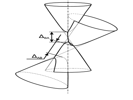
where $\vec{\sigma}_{2D}^{AB}=\left(\Sigma_{rel}^{x}\right)_{BA}\vec{\sigma}_{2D}\left(\Sigma_{rel}^{x}\right)_{BA}^{-1}$, $\vec{p}_{BA}\widehat{\tilde{\chi}^{\dagger}_{-\sigma_{{}_{A}}}}=\left(\Sigma_{rel}^{x}\right)_{BA}\vec{p}\,\left(\Sigma_{rel}^{x}\right)_{BA}^{-1}\widehat{\tilde{\chi}^{\dagger}_{-\sigma_{{}_{A}}}}$. Due to the fact that $\left(\Sigma_{rel}^{x}\right)_{BA}\neq\left(\Sigma_{rel}^{x}\right)_{AB}$, the vector $\vec{p}_{BA}$ of the Dirac cone axis is somehow rotated in respect to the vector $\vec{p}_{AB}$ of its replica as qualitatively shown in Fig. 2. We investigate this in detail a bit later.

The term with a scalar product $\vec{q}\cdot(\vec{K}_{A}+\vec{K}_{B})$ in eq.  (127) shifts equally the bands of quasi-particles, whereas the term with the vector product leads to different sign of shift for bands of electrons and holes due to the presence of $\sigma_{z}$. The pseudo-mass $m_{-}$ (110) with corrections on these shifts leads to appearance of an energy gap $\Delta_{BA}$ between valent and conduction Dirac zones (Fig. 2). By analogy, the pseudo-mass $m_{+}$ (112) with corrections on these shifts leads to appearance of an energy gap $\Delta_{AB}$, $\Delta_{AB}>\Delta_{BA}$ between valent and conduction zones of the Dirac replica (see Fig. 2).

Figure 2: Qualitative representation of splitting for double-degenerated Dirac cone.

As one can see from Fig. 2, the conduction zone of the replica leads to the gap between valent and conduction zones of the primary Dirac cone. Therefore, in spite of the gap, the monolayer graphene is semimetal. This theoretically predicted effect can explains qualitatively the high-intensity narrow strip connecting the valence and the conduction band of graphene in the vicinity of the Dirac point, which has been experimentally observed in ARPES spectra of the monolayer epitaxial graphene on SiC(0001) [15, 16].

Besides, due to diagonality of the Pauli matrix $\sigma_{z}$, a mixing of waves $\Psi_{K_{A}}$ and $\Psi_{K_{B}}$ takes place.

In real experiments investigating the electron motion in the vicinity of the corners $K_{A},\ K_{B}$ of the graphene Brillouin zone, the value of $q$ is not an infinitely small but gets some finite though small values. Therefore, the effect of solutions mixing in the vicinity of points $K_{A},\ K_{B}$ is always presented though it could be small enough. According the results (109, 111) of the previous section, the effect of the mixing is a manifestation of the graphene lattice anisotropy. To existing physical systems whose properties are strongly depended on the presence of graphene lattice anisotropy one can refers to graphene nanoribbons with zigzag and armchair edges, including carbon nanotubes [26, 27, 28]. It is stipulated by the fact that, due to the finite width, these systems effectively represent quasi-one-dimensional configurational ones [29, 30]. The maximal mixing effect should be expected for charge carriers motion in graphene nanoribbons with zigzag and armchair edges.

Thus, the proposed graphene model can qualitatively explain experimentally observed different electrical conductivity of zigzag and armchair graphene nanoribbons as a result of electron-holes asymmetry of graphene.

Now let us estimate the effects stipuleter by the Fermi velocity operator $\hat{v}_{F}$.

10 Approximation of $\pi$ (p_z) electrons

We consider electrons in monolayer graphene in commanly used assumption on the absence of mixing of states for Dirac points $K_{A}$ and $K_{B}$. Then the eq. (131) and eq.

$$\vec{\sigma}_{2D}^{BA}\cdot\vec{p}_{AB}\widehat{\tilde{\chi}^{\dagger}_{+\sigma_{{}_{B}}}}(\vec{r})\left|0,-\sigma\right>=E_{qu}(p)\widehat{\tilde{\chi}^{\dagger}_{+\sigma_{{}_{B}}}}(\vec{r})\left|0,-\sigma\right>,\ q\ll 1$$ (132)

describe the delocalized $\pi$-electron on a Dirac cone and its replicas. Here $\vec{\sigma}_{2D}^{BA}=\left(\Sigma_{rel}^{x}\right)_{AB}\vec{\sigma}_{2D}\left(\Sigma_{rel}^{x}\right)_{AB}^{-1}$, $\vec{p}_{AB}\widehat{\tilde{\chi}^{\dagger}_{+\sigma_{{}_{B}}}}=\left(\Sigma_{rel}^{x}\right)_{AB}\vec{p}\,\left(\Sigma_{rel}^{x}\right)_{AB}^{-1}\widehat{\tilde{\chi}^{\dagger}_{+\sigma_{{}_{B}}}}$,

$\widehat{\tilde{\chi}^{\dagger}_{+\sigma_{{}_{B}}}}(\vec{r})\left|0,\sigma\right>=\left(\Sigma_{rel}^{x}\right)_{AB}\widehat{\chi^{\dagger}_{+\sigma_{{}_{B}}}}(\vec{r})\left|0,\sigma\right>$.

We write down wave functions $\phi_{\uparrow}$ and $\phi_{\downarrow}$ with spin “up” and “donwn” appropriately in the form

$$\phi_{\uparrow}={1\over\sqrt{2}}\left(\begin{array}[]{c}\phi_{1}\\ 0\end{array}\right),\qquad\phi_{\downarrow}={1\over\sqrt{2}}\left(\begin{array}[]{c}0\\ \phi_{2}\end{array}\right).$$ (137)

To obtain numerical estimate but without full scale ab initio simulations we restrict ourselves by consideration of non-selfconsistence problem. With this in mind, the bispinor wave functions of quasi-particles (in the vicinity of Dirac cone) are presented as (almost) free massless Dirac field (p_z-electrons):

$$\left(\begin{array}[]{c}\widehat{\chi^{\dagger}_{-\sigma_{{}_{A(B)}}}}(\vec{r})\left|0,-\sigma\right>\\ \widehat{\chi^{\dagger}_{\sigma_{{}_{B(A)}}}}(\vec{r})\left|0,\sigma\right>\end{array}\right)={e^{-\imath(\vec{K}_{A(B)}-\vec{q})\cdot\vec{r}}\over\sqrt{2}}\left(\begin{array}[]{c}\exp\{-\imath\theta_{k_{A(B)}}\}\phi_{1}\\ \exp\{-\imath\theta_{k_{A(B)}}\}\phi_{2}\\ -\exp\{\imath\theta_{k_{B(A)}}\}\phi_{2}\\ \exp\{\imath\theta_{k_{B(A)}}\}\phi_{1}\end{array}\right)$$ (144)

$$\equiv\left(\begin{array}[]{c}\chi_{-\sigma_{A(B)}}\\ \chi_{+\sigma_{B(A)}}\end{array}\right),$$ (147)

$$\left(\begin{array}[]{c}\widehat{\chi^{\dagger}_{+\sigma_{{}_{A(B)}}}}(\vec{r})\left|0,\sigma\right>\\ \widehat{\chi^{\dagger}_{-\sigma_{{}_{B(A)}}}}(\vec{r})\left|0,-\sigma\right>\end{array}\right)={e^{-\imath(\vec{K}_{A(B)}-\vec{q})\cdot\vec{r}}\over\sqrt{2}}\left(\begin{array}[]{c}-\exp\{\imath\theta_{k_{A(B)}}\}\phi_{2}\\ \exp\{\imath\theta_{k_{A(B)}}\}\phi_{1}\\ \exp\{-\imath\theta_{k_{B(A)}}\}\phi_{1}\\ \exp\{-\imath\theta_{k_{B(A)}}\}\phi_{2}\end{array}\right)$$ (154)

$$\equiv\left(\begin{array}[]{c}\chi_{+\sigma_{A(B)}}\\ \chi_{-\sigma_{B(A)}}\end{array}\right)$$ (157)

where

$$\phi_{i}={1\over(2\pi)^{3/2}\sqrt{N/2}}\sum_{\vec{R}^{A(B)}_{l}}\exp\{\imath[\vec{K}_{A(B)}-\vec{q}\,]\cdot[\vec{R}^{A(B)}_{l}-\vec{r}]\}\psi_{\{n_{i}\}}(\vec{r}-\vec{R}^{A(B)}_{l}).$$ (158)

This form is coherent with known scattering problem considerations [32] when all $\phi_{i}$ should be placed as unity.

Then, in accord with formulas (147, 157) the expression for the wave function (48) is transformed into the following

$$\widehat{\chi}^{\dagger}_{-\sigma_{i^{\prime}}{{}^{A}}}(\vec{r})\equiv\widehat{\chi^{\dagger}_{-\sigma_{{}_{A}}}}(\vec{r}),\quad\widehat{\chi}^{\dagger}_{\sigma_{i}{{}^{B}}}(\vec{r})\equiv\widehat{\chi^{\dagger}_{\sigma_{{}_{B}}}}(\vec{r})\mbox{ for }\forall\ i,\ i^{\prime}.$$ (159)

Now, it is possible to write down matrices $\left(\Sigma_{rel}^{x}\right)_{AB}\approx\Sigma_{AB}$ and $\left(\Sigma_{rel}^{x}\right)_{BA}\approx\Sigma_{BA}$ without sef-action, e.g. for $\Sigma_{AB}$ as:

$$\left(\Sigma_{rel}^{x}\right)_{AB}\widehat{\chi^{\dagger}_{+\sigma_{{}_{B}}}}(\vec{r})\left|0,\sigma\right>\approx\Sigma_{AB}\ \chi_{\sigma_{B}}=\sum_{i=1}^{N_{v}N-1}\int d\vec{r}_{i}$$

$$\times V(\vec{r}_{i}-\vec{r})\left[\chi_{-\sigma_{A}}(\vec{r}_{i})\cdot\chi_{-\sigma_{B}}^{*}(\vec{r}_{i})\right]\chi_{+\sigma_{B}}(\vec{r})={1\over 2^{3/2}}\sum_{i=1}^{N_{v}N-1}\int d\vec{r}_{i}V(\vec{r}_{i}-\vec{r})$$

$$\times\left[\begin{array}[]{cc}e^{-\imath\theta_{k_{A}}}\phi_{1}(\vec{r}_{i})e^{\imath\theta_{k_{B}}}\phi^{*}_{1}(\vec{r}_{i})&e^{-\imath\theta_{k_{A}}}\phi_{1}(\vec{r}_{i})e^{\imath\theta_{k_{B}}}\phi^{*}_{2}(\vec{r}_{i})\\ e^{-\imath\theta_{k_{A}}}\phi_{2}(\vec{r}_{i})e^{\imath\theta_{k_{B}}}\phi^{*}_{1}(\vec{r}_{i})&e^{-\imath\theta_{k_{A}}}\phi_{2}(\vec{r}_{i})e^{\imath\theta_{k_{B}}}\phi^{*}_{2}(\vec{r}_{i})\end{array}\right]\left[\begin{array}[]{c}-e^{-\imath[(\vec{K}_{A}-\vec{q})\cdot\vec{r}-\theta_{k_{B}}]}\phi_{2}(\vec{r})\\ e^{-\imath[(\vec{K}_{A}-\vec{q})\cdot\vec{r}-\theta_{k_{B}}]}\phi_{1}(\vec{r})\end{array}\right],$$ (164)

and similar expression for $\Sigma_{BA}$.

Now we use the tight-bidning approximation for further simplification of $\Sigma_{AB}$ and $\Sigma_{BA}$ matrices. Accounting only nearest neighbors and choosing $\psi_{\{n_{2}\}},\ \psi_{\{n_{1}\}}$ as orbitals of $\pi$-electron:

$$\psi_{\{n_{2}\}}=c_{1}\psi_{\mbox{\small p}_{z}}(\vec{r}\pm\vec{\delta}_{i})+c_{2}\psi_{\mbox{\small p}_{z}}(\vec{r}),\sum_{i=1}^{2}c_{i}=1;\ \psi_{\{n_{1}\}}=\psi_{\mbox{\small p}_{z}}(\vec{r}),$$

after some algebra we gets

$$\Sigma_{AB}={1\over\sqrt{2}(2\pi)^{3}}e^{-\imath(\theta_{k_{A}}-\theta_{k_{B}})}\sum_{i=1}^{3}\exp\{\imath[\vec{K}_{A}-\vec{q}\,]\cdot\vec{\delta}_{i}\}\int V(\vec{r})d\vec{r}$$

$$\times\left(\begin{array}[]{cc}\sqrt{2}\psi_{\mbox{\small p}_{z}}(\vec{r})\psi^{*}_{\mbox{\small p}_{z},-\vec{\delta}_{i}}(\vec{r})&\psi_{\mbox{\small p}_{z}}(\vec{r})[\psi^{*}_{\mbox{\small p}_{z}}(\vec{r})+\psi^{*}_{\mbox{\small p}_{z},-\vec{\delta}_{i}}(\vec{r})]\\ \psi^{*}_{\mbox{\small p}_{z},-\vec{\delta}_{i}}(\vec{r})[\psi_{\mbox{\small p}_{z},\vec{\delta}_{i}}(\vec{r})+\psi_{\mbox{\small p}_{z}}(\vec{r})]&{[\psi_{\mbox{\small p}_{z},\vec{\delta}_{i}}(\vec{r})+\psi_{\mbox{\small p}_{z}}(\vec{r})][\psi^{*}_{\mbox{\small p}_{z}}(\vec{r})+\psi^{*}_{\mbox{\small p}_{z},-\vec{\delta}_{i}}(\vec{r})]\over\sqrt{2}}\end{array}\right),$$ (168)

(169)

$$\Sigma_{BA}={1\over\sqrt{2}(2\pi)^{3}}e^{-\imath(\theta_{k_{A}}-\theta_{k_{B}})}\sum_{i=1}^{3}\exp\{\imath[\vec{K}_{A}-\vec{q}\,]\cdot\vec{\delta}_{i}\}\int V({\vec{r}})d{\vec{r}}$$

$$\times\left(\begin{array}[]{cc}{[\psi_{\mbox{\small p}_{z},\vec{\delta}_{i}}(\vec{r})+\psi_{\mbox{\small p}_{z}}(\vec{r})][\psi^{*}_{\mbox{\small p}_{z}}(\vec{r})+\psi^{*}_{\mbox{\small p}_{z},-\vec{\delta}_{i}}(\vec{r})]\over\sqrt{2}}&-\psi^{*}_{\mbox{\small p}_{z},-\vec{\delta}_{i}}(\vec{r})[\psi_{\mbox{\small p}_{z},\vec{\delta}_{i}}(\vec{r})+\psi_{\mbox{\small p}_{z}}(\vec{r})]\\ -\psi_{\mbox{\small p}_{z}}(\vec{r})[\psi^{*}_{\mbox{\small p}_{z}}(\vec{r})+\psi^{*}_{\mbox{\small p}_{z},-\vec{\delta}_{i}}(\vec{r})]&\sqrt{2}\psi_{\mbox{\small p}_{z}}(\vec{r})\psi^{*}_{\mbox{\small p}_{z},-\vec{\delta}_{i}}(\vec{r})\end{array}\right).$$ (172)

Here $c_{1}=c_{2}=1/\sqrt{2}$, we choose the upper sign for $\pi$-orbital $\psi_{\{n_{2}\}}$ and introduce a notion $\psi_{\mbox{\small p}_{z},\ \pm\vec{\delta}_{i}}(\vec{r}_{2D})=\psi_{\mbox{\small p}_{z}}(\vec{r}_{2D}\pm\vec{\delta}_{i})$.

Substituting known expression for eigenfunctions of hydrogen-like atom, evaluating integrals we obtain rather lengthly ($\vec{q}$)-dependent invertible matrices, for $q=0$ they are pure numeric and up to a common scalar prefactor read

$$\Sigma_{AB}(\vec{K}_{A})=\left(\begin{array}[]{cc}-0.88&-4.3\\ -1.4&-4.1\end{array}\right)$$ (176)

$$\Sigma_{BA}(\vec{K}_{A})=\left(\begin{array}[]{cc}-4.1&1.4\\ 4.3&-0.88\end{array}\right).$$ (179)

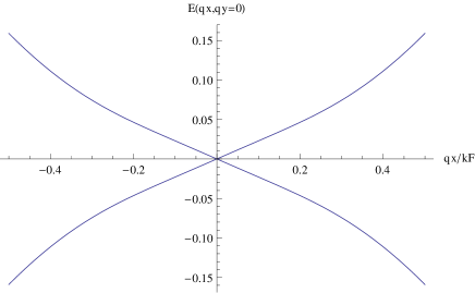
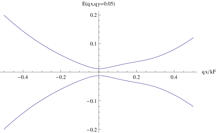
(a)                                                              (b)
     
 
                                                                       (c)  

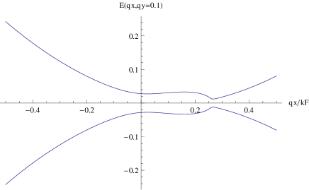
Figure 3: The dependence $E(q_{x},q_{y})$ for several different values of $q_{y}$: (a) – $q_{y}/k_{F}=0$, (b) – $q_{y}/k_{F}=0.05$, (c) – $q_{y}/k_{F}=0.1$

Taking into account the validity condition for our approximation $|\vec{q}|\ll 1$, performing series expansion on $\vec{q}$ up to a linear terms, we get e.g. for $\Sigma_{AB}$.

$$\Sigma_{AB}$$

$$=\left(\begin{array}[]{cc}(0.43+0.33i){q_{x}}+(0.25-0.57i){q_{y}}-0.88&(2.1+1.6i){q_{x}}+(1.2-2.8i){q_{y}}-4.3\\ (0.74+0.73i){q_{x}}+(0.43-1.3i){q_{y}}-1.4&(2.0+1.7i){q_{x}}+(1.2-2.9i){q_{y}}-4.1\end{array}\right).$$ (182)

The most interesting thing in (10) is that eigenvalue problem (132) gives precisely the known dispersion laws $E(\vec{q})=\pm\sqrt{q_{x}^{2}+q_{y}^{2}}$, that is problem is persistent for linear in $|\vec{q}|$ variations.

Now, we take into account higher order in $|\vec{q}|$ terms when evaluating $\Sigma_{AB},\ \Sigma_{BA}$. The spectrum corresponding to eq. (132) deviates from the conic form, that we demonstrate by $E(\vec{q})$ surface sections for few $q_{y}$ in Fig. 3. Fig. 3a emphasizes that in the vicinity of Dirac point the cone is persistent due to symmetry (section crosses original cone and its replicas simultaneously), at higher values of $q$, higher order corrections start to contribute. When section crosses original cone only (Fig. 3b) we find higher order corrections to charge carrier asymmetry. In Fig. 3c we can observe the dispersion curve corresponded to the section crossing original Dirac cone and one of its replicas. We can estimate the $q$-distance between the $K_{A}$ point and one of its reflexes in ARPES experiments as a distance from the origin to $q_{x}$ value corresponded to the local curve minimum near $q_{x}/k_{F}=0.27$ (and minigap $E_{mg}\approx 0.02\ k_{F}v_{F}$), but of course, approximations we made were too rough to obtain a credible result, it should be considered as qualitative only.

As it has been shown above divergence of Dirac cone and its replicas relative to each other leads to the electron-hole asymmetry. Then, the six fold rotational symmetry of graphene near the Dirac point energy breaks. The displacement of replicas points in the graphene Brillouin zone on respect to the primary Dirac cone points occurs on a distance

$$|\Delta\vec{q}_{AB}|=|\vec{q}_{AB}-\vec{q}_{BA}|.$$ (184)

Since in the neighborhood of the top of the Dirac cone $q\to 0$, and (as was shown above) the cone persists then, in accord with (184) in the graphene Brillouin zone all points of the Dirac cone replicas shift, except of their tops (see Fig. 4).

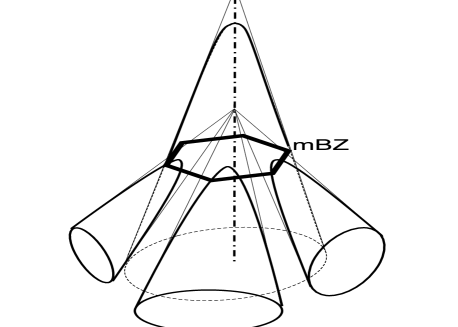
Figure 4: Mini Brillouin zone (mBZ) formed from the Dirac cone replicas in the vicinity of the primary Dirac cone. Three of six replicas are shown.

To understand what numerical value it could correspond to, we choose $\vec{q}\propto\vec{K}_{A}$ and find $\Delta\vec{q}_{AB}$ based on (184) and expressions (176, 179) for $\Sigma_{BA},\Sigma_{AB}$. Then the rotation angle $\alpha=\arccos\left(\vec{q}_{AB}\cdot\vec{q}_{BA}/|\vec{q}_{AB}||\vec{q}_{BA}|\right)\approx\pi/2$, so such a rotation could be large enough for some points in momentum space.

Thus, the removal of the degeneracy leads to the appearance of the hexagonal mini Brillouin zone in the vicinity of the Dirac point, such that the corners of the cones lie on the same line, whereas the replicas are rotated with respect to Dirac cone (Fig. 4, 5).

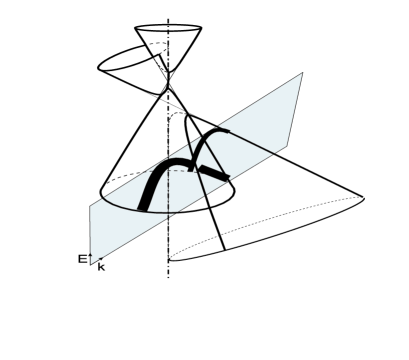
Figure 5: ARPES experimental plane(shaded) cuts the valent zone and its replica in the vicinity of the Dirac point $K_{A(B)}$. Lines at intersection mark the ARPES band (thick line) and its replica (less thick line).

The electron density distribution is unstable at the intersection of the cones of the mini Brillouin bands with the Dirac cone of the graphene Brillouin zone. Therefore, in these places the Dirac cone and its replicas can only quasi-cross to form energy mini-gaps in the ARPES band as shown in Fig. 5. Since $\Delta_{BA}<\Delta_{AB}$, the probability of transitions for replica photoelectrons is lower than for photoelectrons near the Dirac cone. This fact is represented in Fig. 5 by lines at the intersection of the valent zones with ARPES experimental plane which have different intensities (shown in the figure by different thicknesses). The more intensive line (thick) represents the ARPES band for photoelectrons near the Dirac cone.

Mini-gaps in the vicinity of the Dirac point has been experimentally observed as minigaps ($<0.2$ eV) in asymmetrical photoemission intensity of ARPES spectra for weakly interacting graphene on iridium support [14].

11 Conclusion

To summarize, application of secondary quantized self-consistent Dirac – Hartree – Fock approach to consider electronic properties of monolayer graphene with accounting of spin-polarized states allows to coherently explain experimental results on energy band minigaps and charge carrier asymmetry in graphene, propose a description of valent and conduction zones shifts and gives a nice theoretical estimation of electron and holes cyclotron masses which is in very good agreement with known experimental data.

References

[1] Wallace, P. R. 1947. The Band Theory of Graphite.
Phys.Rev. 71:622-634.
[2]
Semenoff, G.W. 1984. Condensed-matter simulation of a three-dimensional
anomaly. Phys. Rev. Lett. 53:2449.
[3]
Saito, R. G. 1998. Physical Properties of Carbon Nanotubes. London: Imperial.
[4]
Reich, S. et al. 2002. Tight-binding description of
graphene. Phys. Rev. B. 66:035412.
[5]
Novoselov, K.S. et al. 2005. Two-dimensional gas of massles Dirac fermions in graphene.
Nature 438:197-200.
[6]
Zhang, Y. et al. 2005. Experimental observation of the quantum Hall effect and
Berry’s phase in graphene. Nature 438:201-204.
[7]
Deacon, R.S. et al. 2007. Phys.Rev. B. 76:081406(R).
[8]
Jiang, Z. et al. 2007. Phys. Rev. Lett. 98:197403.
[9] Rojas-Cuervo, A. M., R. R. Rey-González.
2013. Asymmetric Dirac cones in monatomic hexagonal lattices. arXiv:
1304.4576v1 [cond-mat.mes-hall] 16 Apr 2013.
[10] Altshuler, B.L., B.Z. Spivak. 1985.
Change of random potential realization and conductivity of small
size sample. JETP Lett. 42:447.
[11] Rossi, E. et al.
2012.
Universal conductance fluctuations in Dirac materials in the presence of
long-range disorder. Phys. Rev. Lett. 109:096801.
[12] Rahman, Atikur et al. 2013. Asymmetric scattering of Dirac electrons and holes in graphene.
arXiv:1304.6318v1 [cond-mat.mes-hall] 23 Apr 2013.
[13]
Rahman, Atikur et al. 2013. Direct evidence of angle-selective transmission of Dirac electrons in
graphene p-n junctions. arXiv:1304.5533v1 [cond-mat.mes-hall] 19 Apr 2013.
[14]
Pletikosić, I. et al. 2009. Dirac Cones and Minigaps for Graphene on Ir(111).
Phys. Rev. Lett. 102:056808,
arXiv: 0807.2770v2 [cond-mat.mtrl-sci] 13 Feb 2009.
[15]
Zhou, S.Y. et al. 2008. Origin of the energy bandgap in epitaxial graphene.
Nature Mater. 7:259-260.
[16] Zhou, S.Y. et al.
2007. Substrate-induced band
gap opening in epitaxial graphene. Nature Mater. 6:770,
preprint at arXiv:0709.1706v2.
[17]
Castro Neto, A.H. et al. 2009. The electronic properties of graphene.
Rev. Mod. Phys. 81:109-162.
[18]
N M R Peres, 2009.
The transport properties of graphene
J. Phys.: Condens. Matter 21: 323201 (10pp)
[19] Reich, S. et al.
2002. Electronic band structure of isolated and
bundled carbon nanotubes. Phys. Rev.B. 65:155411.
[20]
Grushevskaya, G. V. et al. 1998. Exchange
and correlation interactions and band structure of
non-close-packed solids. Physics of the solid state. 40:1802-1805.
[22]
Krylov, G.G., H.V. Krylova, M.A. Belov. 2011. Electron transport in
low-dimensional sysyems: localization effects. In Dynamical phenomena in complex systems, ed. A.V. Mokshin et al.,
161-180. Kazan: Publishing MOiN RT.
[23]
Grushevskaya, G. V. and G.G. Krylov. 2013.
Charge Carriers Asymmetry and Energy Minigaps in Monolayer
Graphene: Dirac Hartree Fock approach. Nonlinear Phen. in
Comp. Sys. 16: 189-208.
[24]
V.A. Fock. 1931. Foundations of quantum mechanics. Moscow: Science Publisher, 1976 (in Russian).
[26]
Brey, L., H. Fertig. 2006. Phys. Rev. B. 73:195408;
2006. Phys. Rev. B. 73:235411.
[27]
Nakada, K. et al. 1996. Phys.Rev. B. 54:17954.
[28] Maksimenko, S.A., G. Ya. Slepyan.
2003. Electromagnetics of carbon nanotubes. In Introduction to
complex medium for optics and electromagnetics, ed. W.S.
Wieglhofer, A. Lakhtakia, 507-545. Bellingham: SPIE Press.
[29]
Krylova, H.V. 2008. Electric charge transport and nonlinear polarization
of periodically packed structures in strong electromagnetic fields.
Minsk: Publishing Center of BSU.
[30]
Krylova, Halina, Leonid Hursky. 2013. Spin polarization in
strong-correlated nanosystems.
Germany: LAP LAMBERT Academic Publishing, AV Akademikerverlag GmbH & Co.
[31] Katsnelson, M. I. 2006. Zitterbewegung, chirality,
and minimal conductivity in graphene. Eur. Phys. J.
B 51:157 160.
[32] Katsnelson, M. I.
et al. 2006. Chiral tunneling and the Klein paradox in graphene
Nature Physics. 2:620-625.
[33] Katsnelson, M. I. 2007. Graphene: carbon in two
dimensions. Materials Today. 10:20-27.