Evolution in biology Complex systems Structure and organization in complex systems

Evolution and non-equilibrium physics. A study of the Tangled Nature Model

Abstract

We argue that the stochastic dynamics of interacting agents which replicate, mutate and die constitutes a non-equilibrium physical process akin to aging in complex materials. Specifically, our study uses extensive computer simulations of the Tangled Nature Model (TNM) of biological evolution to show that punctuated equilibria successively generated by the model’s dynamics have increasing entropy and are separated by increasing entropic barriers. We further show that these states are organized in a hierarchy and that limiting the values of possible interactions to a finite interval leads to stationary fluctuations within a component of the latter. A coarse-grained description based on the temporal statistics of quakes, the events leading from one component of the hierarchy to the next, accounts for the logarithmic growth of the population and the decaying rate of change of macroscopic variables. Finally, we question the role of fitness in large scale evolution models and speculate on the possible evolutionary role of rejuvenation and memory effects.

Introduction. Initially perceived as a challenge to gradualism, punctuated equilibria are now widely accepted [1, 2] as key features of large scale darwinian evolution. Their striking similarity to intermittency in ‘aging’ [3, 4, 5, 6] complex materials is not well understood, but may hold clues on how life evolves from matter [7]. The origin of this similarity is addressed below by analyzing the Tangled Nature Model (TNM) dynamics [8, 9] as a non-equilibrium physical process.

While physics ideas are common in evolution models [10, 11], evolution itself has not previously been modeled as a physical process, bar attempts [12, 13, 14] inspired by Self Organized Criticality (SOC) [15], according to which punctuations are the manifestation of stationary fluctuations. We see them instead as the manifestation of a spontaneous physical process. But how can a pertinent free energy then be defined and why does the process decelerate over time [16, 17]?

In spite of its simplicity, the TNM, an individual based stochastic model of ecosystem dynamics, captures key aspects of co-evolution, e.g. its decelerating nature [18], its log-normal species abundance distribution [19] and, in a version including spatial migration, the area law [20]. Punctuations, here called quakes, irreversibly disrupt quasi-Evolutionary Stable Strategies (qESS), periods of metastability where population and the number of extant species, or diversity, fluctuate reversibly. Statistical physics is used to connect microscopic interactions, defined in darwinian terms at the level of individuals, to macroscopic properties, e.g. population and diversity. Along the way, we introduce the concepts of core and cloud species and implement an adaptation of the lid method [21] originally developed to map out complex energy landscapes. We find that: i) The growing duration of qESS reflects an entrenchment into metastable configuration space components of increasing entropy; ii) The decreasing rate of evolution stems from a logarithmic time growth of the entropic barriers separating successive qESS; iii) Rare fluctuations in a time series of positive couplings extending from the core to the cloud trigger the quakes. The physical picture emerging highlights the similarity of evolution and physical aging of complex materials. The ubiquitous role of hierarchies in complex dynamics [22, 23] suggests that similar conclusions might hold beyond the TNM.

Background. Our results are based on simulations performed at the SDU horseshoe cluster, using C code developed from scratch. Detailed information on the model parameters, the initial conditions, and how to generate the couplings can be found in Ref. [9], which should be consulted for further details. For convenience, some definitions and known properties are given below.

The TNM’s variables are binary strings of length $K$, i.e. points of the $K$ dimensional hypercube. Variously called species or sites, these are populated by agents or individuals, which reproduce asexually in a way occasionally affected by random mutations. Only a tiny fraction of the possible species ever becomes populated during simulations lasting up to one million generations. The extant species, i.e. those with non-zero populations at a given time, are collectively referred to as ecosystem, and their number as diversity. With probability $\theta$, a pair $(a,b)$ of species has non-zero couplings, ($J_{ab}$, $J_{ba}$), describing how $b$ affects the reproductive ability of $a$ and vice-versa. Empirically, the distribution of the generated couplings is well described by the Laplace double exponential density $p(x)=\frac{1}{2a}e^{-\lvert x-\overline{x}\rvert/a}.$ The parameters $\overline{x}$ and $a$ are estimated to $-0.0019$ and $0.0111$, respectively. Extant species cluster together, their closeness expressed by the Hamming distance, the number of bits by which their strings differ.

Let $\mathcal{S}$, $N_{b}(t)$ and $N$ denote the ecosystem, the population size of species $b$, and the total population $N(t)=\sum_{b}N_{b}(t)$. An individual of type $a$ is chosen for reproduction with probability $n_{a}=N_{a}/N$, and succeeds with probability $p_{\rm off}(a)=1/(1+e^{-H_{a}})$, where

$$H_{a}(t)=-\mu N(t)+\sum_{b}j_{ab}(t),$$ (1)

and where

$$j_{ab}=\frac{N_{b}}{N}J_{ab}=J_{ab}n_{b}$$ (2)

is a density weighted coupling. In Eq. (1), $\mu$ is a positive constant. Letting $p_{\rm mut}$ be the mutation probability per bit, parent and offspring differ by $k$ bits with probability Bin$(k;K,p_{\rm mut})$, the binomial distribution. Death occurs with probability $p_{\rm kill}$ and time is given in generations, each equal to the number of updates needed for all extant individuals to die. Thus, with population $N$ at the end of the preceding generation, the upcoming generation comprises $Np_{\rm kill}$ updates. The parameters used are always $K=20$, $\mu=0.10$, $\theta=0.25$, $p_{\rm kill}=0.20$, $p_{\rm mut}=0.01$, and the initial condition invariably consists of a single species populated with 500 individuals.

Core and cloud. Core species have, by our definition, sizes exceeding $5$% of the most populous species. All together, they make up about 80% of the population. Other extant species, dubbed cloud species, are sparsely populated, mainly by mutants of neighboring core species. A three dimensional visualization of the ecosystem is shown in Fig. 1 after $10^{3},\;10^{5}$ and $10^{7}$ generations, with core and cloud species marked by red squares and gray circles, respectively. Each core species is surrounded by its own cloud and both the number of core species and their distance, which reflects the Hamming distance, are seen to gradually increase as the system ages.

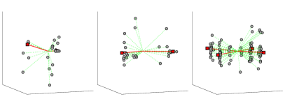
Figure 1: Core (red squares ) and cloud (gray circles) species at different system ages. All graphs drawn on the same scale. The red lines are guides to the eye, showing the growing separation between core species.

Every panel of Fig. 2 depicts the Probability Density Function (PDF) of the density weighted couplings, see Eq. (2), after $t=5\cdot 10^{3}$, $t=8\cdot 10^{4}$ and $t=10^{6}$ generations. The corresponding data are sampled within qESS, where core and cloud are well defined.

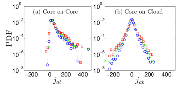
Figure 2: PDF of density weighted couplings: $t=5\cdot 10^{3}$ (red squares), $t=8\cdot 10^{4}$ (green crosses), $t=10^{6}$ (blue circles).

Panel $(a)$ shows that negative couplings connecting core species are rare in a young system and then disappear. Hence, couplings do not specify trophic chains: A predator and prey species stabilizing each other can interact positively, while competing predators can interact negatively. Couplings extending from core to cloud, panel $(b)$, feature a nearly symmetric PDF whose width decreases with age. Core to cloud and cloud to cloud couplings have PDFs (not shown) similar to those of arbitrary species.

Entropy, entropic barriers and hierarchies. In some thermalizing complex systems, increasing energy barriers $b_{n},\;n=0,1,\ldots$ separate the nested metastable components of a dynamical hierarchy, see e.g. [3, 24]. When starting out in state $x_{0}$, surmounting the $n$’th barrier gives access to a component ${\cal V}_{n}$ whose volume increases exponentially with $n$. To map out this situation, the lid method [21] introduces artificial and impenetrable energy barriers called ‘lids’, which allow the system to fully equilibrate in the sub-volume of configuration space below the lid. As we argue, a similar description holds for the TNM, with energy barriers replaced by entropic ones.

The configuration volume ${\cal V}$ associated to a qESS with $V$ extant cloud species and $N_{\rm cloud}$ individuals scattered among them is approximately ${\cal V}\approx V^{N_{\rm cloud}}$. This formula includes the (unlikely) case where all cloud individuals belong to the same species, which contradicts the definition of cloud species. Secondly, the core only serves to label the qESS and the entropic contribution from its (few) configurations is neglected. The configurational entropy is then $S=\log({\cal V})\approx N_{\rm cloud}\log(V)$, where $V$ can be estimated via the quantity $\overline{\langle d_{\rm H}\rangle}$, obtained by averaging the mean distance $\langle d_{\rm H}\rangle$ of cloud species to the most populous core species over the available ensemble of $2022$ trajectories. To a good approximation, the number of vertices at distance $k\ll K$ from a given vertex increases exponentially, leading to $V(t)\approx\exp(\overline{\langle d_{\rm H}\rangle}/K)$. As shown in Fig. 3, $\overline{\langle d_{\rm H}\rangle}\propto\log(t)$. Furthermore, we have checked that $N_{\rm cloud}\propto\log(t)$. Hence, introducing $t$ for the time scale of the qESS, we find

$$S(t)\propto\log(t)^{2}\quad{\rm and}\quad{\cal V}(t)\propto t^{a\log(t)},$$ (3)

where $a$ is a positive constant. As the entropy increases and the free energy correspondingly decreases in time, TNM dynamics qualifies as a spontaneous non-equilibrium physical process. Importantly, the source of disorder lies entirely with the cloud.

As discussed later, the fragility of TNM ecosystems implies that a mutant able to replicate successfully, say mutant $a$, quickly destabilizes the core. Consequently, a quake is triggered whenever $H_{a}\geq 0$, or equivalently, if $\sum_{b\in\mathcal{S}}j_{ab}(t)>\mu N(t)$. The sum runs over all extant species but can safely be restricted to core species. In fact, as a mutant is most probably connected to a single core species $c$, the criterion simplifies to

$$j_{ac}(t)>\mu N(t).$$ (4)

Since $N$ on average increases, Eq. (4) represents a rising bar for mutants to destabilize the existing core.

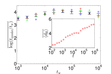
Figure 3: Main plot: The data with $1\sigma$ statistical error bars (black) show the average of $\log(t_{\rm quake}/t_{\rm w})$ vs. $t_{\rm w}$, estimated using $2022$ trajectories. The blue circles, green diamonds and red squares are based on different sub-samplings and illustrate the statistical variation of the data. Insert: Hamming distance from cloud species to the most populous core species, plotted on a log scale and averaged twice: over the cloud species and over $2022$ trajectories.

As anticipated, we now modify the TNM by a ‘lid’ rule: Each time a species $a$ is selected for reproduction, any coupling $J_{ab}$ entering $H_{a}$ and exceeding a preset value $L$ is set equal to $L$. Equation (4) then entails $N(t)\leq L/\mu$. Figure 4 shows that our lid rule halts the evolutionary drift of the TNM, with the stable levels of population and diversity reached depending on the size of the lid but not on the time of its deployment. Refs. [25, 26, 27, 28, 29], to which we shall return, report and analyze similar stationery fluctuation patterns.

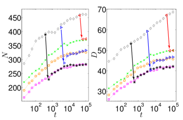
Figure 4: The two upper curves show: Left panel, the average population, divided by two for graphical reasons, right panel, the diversity, both plotted vs. time. Lower curves: same quantities with initially imposed lids. $L=50,60$ and $70$ from bottom to top. Arrows show the fast decays which ensue when the same lids are imposed at times $t=5\cdot 10^{2},10^{3}$ and $10^{4}$.

To estimate the level $N_{L}$ at which the population settles, let $|{\mathcal{C}}|$ be the size of the core and set $J_{c^{\prime}c}=L$, the highest value compatible with $J_{c^{\prime}c}\leq L$ in $H_{c^{\prime}}=\sum_{c=1}^{|{\mathcal{C}}|-1}J_{c^{\prime}c}\;n_{c}-\mu N_{L}\approx 0,$ a slight over-estimate of the typical $H$ value of a stable core species $c$. This yields $N_{L}\approx\frac{Lf_{C}}{\mu},$ where $f_{C}=\sum_{c=1}^{|{\mathcal{C}}|-1}n_{c}$. Based on data from Fig. 4, Table 1 compares the measured population level $N_{L}$ with the estimate $Lf_{C}/\mu$, showing that the latter overestimates $N_{L}$ by approx. 15%.

Lid on the interaction strengths
$t_{\rm lid}$	$L$	$f_{C}$	$N_{L}$	$Lf_{C}/\mu$
0	50	0.641	282	317
0	60	0.626	326	377
0	70	0.620	371	432
5$\cdot 10^{2}$	50	0.638	283	318
5$\cdot 10^{3}$	60	0.627	333	375
5$\cdot 10^{4}$	70	0.614	374	428

Table 1: Columns 1-3: $t_{\rm lid}$ is the time of lid deployment, $L$ is the lid value, $f_{C}$ is the core population fraction. Columns 4-5: the population size $N_{L}$ for lid $L$, as obtained from Fig. 4, and the corresponding estimate.

To see why the lid locks the system size, note that the requirement for destabilization from species $a$, Eq. (4), now reads $J_{ac}n_{c}>\mu N_{L}\approx Lf_{C}$. Since $Ln_{c}>J_{ac}n_{c}$, destabilization requires $n_{c}\geq f_{C}$, which is impossible unless the core contains a single species.

According to Eq. (3), the configuration space volume available to a qESS at time $t$ is ${\cal V}(t)\propto t^{a\log(t)}\propto t^{bN(t)}$, where $a$ and $b$ are positive constants. Furthermore, since the extant population $N$ grows linearly with the lid, the configuration space volume grows exponentially with it. This already implies a hierarchical organization of configuration space, with components mutually inaccessible on a time scale $t^{\prime}$ or, alternatively, for a lid value $L^{\prime}$, merging at $t>t^{\prime}$ or $L>L^{\prime}$. As a further check, we reverse the process to see a component split: Consider a trajectory lasting $10^{4}$ generations. At $t=10^{3}$ a lid $L=50$ is imposed and the system is allowed to relax to a final state, labeled by its largest extant species. The procedure is repeated $200$ times with identical initial state and random seed, but resetting the seed to a different value each time the lid is imposed. To improve the statistics, the whole process is then repeated for $94$ different starting points. In approx. 75% of the cases, more than 180 different end states are reached out of the $200$ possible. In the remaining 25% of the cases, on average 65 different end states are reached. In conclusion, the configuration space component available after $10^{3}$ generations contains a large number of sub-components with different cores.

Quake rate and qESS duration Since no macroscopic changes occur during qESS, a coarse grained description is naturally formulated in terms of Poissonian quake statistics [30] . Furthermore, based on the analysis of Ref. [18], the rate of quakes can be assumed to be $r_{\rm q}(t)=A/t$, where $0<A\leq 1$ is a constant. The condition $A<1$ excludes a partition of the system into statistically independent sub-systems, which is fitting, as all species are coupled through $N(t)$. Let us finally assume that each quake leads to a random population change with average value $\mu_{\Delta}$. The average population after $n$ quakes is then $n\mu_{\Delta}$ which, averaged again over the probability that these quakes occur in the interval $(1,t)$, finally yields

$$N(t)=\mu_{\Delta}A\log(t),$$ (5)

a logarithmic growth in qualitative agreement with our data. An average over the population changes incurred in all quakes yields $\mu_{\Delta}=105$. Using the logarithmic slope $\mu_{\Delta}A$ of the average population growth, fitted for $t>1000$, see Fig. 4, one finds $A=0.28$, which is close to the value $A=0.26$ obtained, as explained below, from the temporal statistics of quakes. Assuming a log-Poisson description for the latter, the average number of quakes in $(t_{\rm w},t)$ is $\mu_{\rm q}(t_{\rm w},t)=A\log(t/t_{\rm w})$, and the probability density for the first quake to happen at time $t>t_{\rm w}$ is $P_{\rm quake}(t_{\rm w},t)=At_{\rm w}^{-1}(t/t_{\rm w})^{-A-1}$. Averaging $\log(t)$ over $P_{\rm quake}$ produces

$$\overline{\log\left(t/t_{\rm w}\right)}=\frac{1}{A}>1.$$ (6)

The fair agreement with the estimate shown in the main plot of Fig. 3 confirms that the quake rate is proportional to $1/t$. Note that the mathematical expectation of the qESS life-time $t-t_{\rm w}$ is undefined, and that the empirical average of the same quantity correspondingly features a huge scatter. For each trajectory, the entropic barrier $\Delta S(t_{\rm w})$ delimiting a qESS is the exponential of its duration. Hence, Eq. (6) implies that the average entropic barrier grows linearly with $\log(t_{\rm w})$.

The main plot of Fig. 3 is obtained by estimating the time $t_{\rm quake}>t_{\rm w}$ at which a core extant at time $t_{\rm w}$ is destroyed by a quake. To this end, a large number of mutants are generated and their ability to destabilize the core assessed. The procedure is carried out for ten $t_{\rm w}$ values equidistant on a logarithmic scale stretching from $10^{3}$ to $10^{6}$ generations. The number of independent trajectories used for each age varies between 907 (old systems) and 1663 (young systems). The variation reflects that, due to the finiteness of the system size, some ecosystems —especially old ones— are infinitely stable, as none of the mutants generated can destabilize them. Stable systems cannot contribute to the quake statistics and are hence discarded.

Mutant $a$ is deemed able to destabilize the core if $H_{a}>5$, or equivalently, if its reproduction probability exceeds $99.3\%$, a slightly more stringent requirement than the $H_{a}>0$ implied by Eq. (4). Glossing over the distinction between repeated and single mutations leading to the same species, and using that core species by far are the main source of mutants, we let $M(l)$ be the total number of species at a distance $l$ from their common core ancestor $c$, and let $m_{c}(l)$ be the number of those able to destabilize the core. Species $c$ is chosen for reproduction with probability $n_{c}$ and succeeds with probability $p_{\rm off}(H_{c})$. The probability of producing a mutant at a distance $l$ is $P(X_{\rm mut}=l)={\rm Bin}(l;K,p_{\rm mut})$ and the likelihood of hitting a destabilizing species under mutation of $c$ is $m_{c}(l)/M(l)$. All the above events being independent, the probability of destabilization per reproduction step at age $t_{\rm w}$ is

$$p_{\rm quake}(t_{\rm w})=\sum_{c\in\mathcal{C}}n_{c}\;p_{\rm off}(H_{c})\sum_{l}P(X_{\rm mut}=l)\frac{m_{c}(l)}{M(l)}.$$ (7)

The outer sum is over all core species and the inner one over all possible distances between mutant and parent species. Destabilization in $t$ attempts follows the geometric distribution with PDF $p_{\rm quake}(t_{\rm w})(1-p_{\rm quake}(t_{\rm w}))^{t-1}$, and the average number of attempts required is thus $1/p_{\rm quake}(t_{\rm w})$. This leads to the estimate

$$t_{\rm quake}(t_{\rm w})=t_{\rm w}+\frac{1}{p_{\rm quake}(t_{\rm w})}$$ (8)

for the time at which a core extant at time $t_{\rm w}$ is destroyed by a quake. Averaging over 2022 independent trajectories the logarithm of $t_{\rm quake}/t_{\rm w}$ yields the main plot in Fig. 3. The estimate $A=0.260\pm 0.002$ is obtained straightforwardly from the latter.

Quake triggering fluctuations. After establishing that a limit on the range of $H_{a}$ stops the evolution of the TNM, we detail how quakes are triggered. To this end, data are needed with a temporal resolution $200$ times higher than in the rest of this work. These data are collected for short intervals straddling the approximate position of the quakes. The procedure is repeated for 100 trajectories lasting up to $10^{5}$ generations and comprising at least $4$ quakes.

To gauge the highest contribution to the $H$ values of the cloud species, we define the time dependent ‘trigger’ function

$$T(t)=\max_{a\in{\rm cloud}}\left\{\sum_{c\in{\rm.core}}J_{ac}n_{c}\right\}-\mu N(t),$$ (9)

depicted as the magenta curve in the inner plot of Fig. 5. Initially fluctuating well below zero, $T$ suddenly jumps above zero at $t=16,096$. Soon thereafter, the population (the gray curve shows the population scaled down for convenience), decreases dramatically, which is a sign of destabilization. A further indication is the clearly visible change in the system’s Center of Mass, (orange curve, also scaled down), the latter obtained by mapping the bit string of each species into a real number and interpreting the corresponding population as a mass. The quake extends from $t=16,096$ to $t=16,119$, a minuscule interval during which $T(t)$ oscillates erratically before returning to the negative values characterizing the new qESS. The situation just described pertains to a single trajectory. To ascertain its general validity, we define a Boolean matrix $B_{i,q}$, where $i$ and $q$ index trajectories and quakes within a trajectory, respectively. For each $i$, $B_{i,q}=1$ if the $q$’th quake is preceded by a positive fluctuation of $T(t)$ and $-1$ if not. Averaging over all trajectories yields the function ${\rm Corr}(q)$ depicted in the main plot of Fig. 5. ${\rm Corr}(q)=1$ would indicate a perfect correlation. The values shown are a bit lower since in rare cases, values of $T(t)$ lingering slightly below zero can trigger quakes.

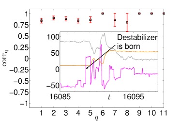
Figure 5: Main plot: Correlation between the first zero crossing of the trigger function $T(t)$ to positive values and a subsequent large change in population and/or Center-of-Mass (COM). Insert: $T(t)$ vs. time, showing its first zero crossing and the concomitant birth of a destabilizer species at $t=16,096$. Also included are traces of population (gray) and COM (orange) scaled down for convenience.

Figure 6 further details how the sudden growth of one mutant species induces a quake. Before $t_{q}\approx 9171$ two stable core species are present. The arrival of a new species (dark green curve) at $t_{q}\approx 9171$ starts a quake which ends in a new stable configuration at $t\approx 9190$. The latter has twice as many core species as the old one and almost twice the population. During the quake many mutants gain population and disappear. The populations of a few of these mutant species are plotted in the figure vs. time, with arrows pointing to the instants at which they appear and again disappear. Quakes are generally short and turbulent periods during which old species disappear and new ones gain foothold. In the present example a species which never had more than 10 individuals manages to destroy a core stable through many generations. The surprising fragility of the TNM ecosystems appears similar to the fragility of real ecosystems with respect to the introduction of new invasive species.

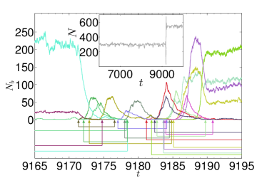
Figure 6: Main plot: The noisy curves show population vs. time for selected species able to reproduce during a quake. Their birth and extinction are marked by color coded vertical arrows connected by horizontal lines. The species appearing at $t_{q}\approx 9171$ (dark green curve) marks the beginning of the end. Insert: the total population vs. time before and after the quake.

Discussion and outlook.

Focusing on the non-stationarity nature of the dynamics, we have placed the TNM in a wide class of hierarchically organized [22] metastable systems, alongside with aging glassy materials [23]. During a qESS the dynamics is stationary within a component of the hierarchy and full stability is achieved by imposing a ‘lid’ curtailing the Laplace distribution of the couplings into one supported in a finite interval. A coupling distribution with finite support, as used in Refs. [8, 25, 26, 27, 28, 29], seems therefore crucial for reaching a stationary regime within accessible time scales. This regime is studied in detail and given a biological interpretation in [25, 26, 27, 28, 29]. An interesting open question concerns the dynamical effect of a broad, e.g. power-law, distribution of couplings,

Hierarchical systems admit a coarse-grained dynamical description in terms of quakes connecting metastable states. These quakes constitute a Poisson process [30], whose average depends on a difference of ‘stretched times’, with the stretching function being a logarithm in the TNM case. Such ‘log-Poisson’ processes arise when quakes are triggered by record breaking fluctuations [30] but can also follow from the gradual increase of dynamical barriers in a hierarchy [23].

Can ‘fitness’ be an emerging property of the TNM? At the individual level the answer is negative by construction. At the systemic level, e.g. the individual level of a coarser description, the only measure of success is long-term core stability. The latter can result from all mutants receiving negative interactions and hence being unable to reproduce. Conversely, depending on whether a core or a cloud species is at the receiving end, positive interactions underlie the stability of the core or cause its eventual demise. Since the interactions linking core species are nearly irrelevant for stability, evolutionary success is not a function of the state of the core. Hence, coarse graining the latter into a ‘compound’ species does not lead to a fitness based evolution model similar to e.g. the Kauffman’s  NKC model [31]. The result more closely resembles a neutral model of evolution, see [32] and references therein, with the proviso that the rate of genetic drift is in our case decelerating if the environment stays constant.

In our log-Poisson description, a qESS has infinite expected life-time, while the expectation value of the logarithm of its duration depends on how long the core has existed. This weak predictive ability is reminiscent of, and might even supply a formal mathematical basis for, the ontic openness [33] of real ecosystems.

The TNM population size depends on $\mu$ and even though a $\mu$-cycle (of moderate amplitude) will eventually restore the population at its original level, we expect that an increase followed by a decrease will modify the core, while the inverse process will leave it unchanged. In other words, the first process lets the system explore new parts of its hierarchical configuration space, similarly to rejuvenation[34, 35], while the second keeps a memory of the past state. Possibly, partial randomization achieved by a periodic variation of the environment can accelerate the pace of evolution and, in the context of the extended TNM with spatial features [20], lead to the formation of new structures at a higher level of aggregation. Finally, since the bit strings of the TNM can code for strategies of economic agents [36], our analysis might be relevant for understanding the optimal balance between continuity and innovation in human societies.

Acknowledgements. P.S. is grateful to Henrik Jeldtoft Jensen and Per Lyngs Hansen for many inspiring discussions and thanks two anonymous referees for their constructive advice.

References

- [1] S.J. Gould and N. Eldredge. Paleobiology, 3:115–151, 1977. S.J. Gould and N. Eldredge. Nature, 366:223–227, 1993.
- [2] S. J. Gould. The Structure of Evolutionary Theory. Belknap Harward, 2002.
- [3] P. Sibani and K.H. Hoffmann. Phys. Rev. Lett., 63:2853–2856, 1989.
- [4] L.P. Oliveira, H. J. Jensen, M. Nicodemi and P. Sibani. Phys. Rev. B, 71:104526, 2005.
- [5] P. Sibani, G.F. Rodriguez and G.G. Kenning. Phys. Rev. B, 74:224407, 2006.
- [6] S. Boettcher and P. Sibani. Journal of Physics: Condensed Matter, 23(6):065103, 2011.
- [7] J. Trefil, H. Morowitz, and E. Smith. American Scientist, 97:206–213, 2009.
- [8] K. Christensen, S.A. de Collobiano, M. Hall, and H.J. Jensen. Journal of Theoretical Biology, 216(1):73–84, 2002.
- [9] P.E. Anderson and H.J. Jensen. Journal of Theoretical Biology, 232::551–558, 2005.
- [10] Andrew J. Black and Alan J. McKane. Trends in Ecology and Evolution, 27, 337-345, 2012.
- [11] B. Drossel. Advances in physics, 50:209–295, 2001.
- [12] P. Bak and K. Sneppen. Phys. Rev. Lett., 71:4083–4086, 1993.
- [13] P. Bak and S. Boettcher. Physica D, 107:143–150, 1997.
- [14] K. Sneppen, P. Bak, and H. Flyvbjerg. Proceedings of the National Academy of Sciences, 92:5209–5213, 1995.
- [15] P. Bak, C. Tang and K. Wiesenfeld. Physical Review Letters, 59:381–384, 1987.
- [16] M. E. J. Newman and P. Sibani. Proceedings of the Royal Society London B, 266:1–7, 1999.
- [17] J. Alroy. PNAS, 105:11536–11542, 2008.
- [18] D. Jones, H.J. Jensen, and P. Sibani. Phys. Rev. E, 82:036121, 2010.
- [19] M. Hall, K. Christensen, S. A. di Collobiano, and H.J. Jensen. Phys. Rev. E, 66:011904, 2002.
- [20] D. Lawson and H.J. Jensen. Journal of Theoretical Biology, 241(3):590–600, 2006.
- [21] P. Sibani, R. van der Pas, and J. C. Schön. Computer Physics Communications, 116:17–27, 1999.
- [22] H. A. Simon. Proc. of the American Philosophical Society, 106:467–482, 1962.
- [23] P. Sibani and H. J. Jensen. Stochastic Dynamics of Complex Systems: from Glasses to Evolution. Imperial College Press, 2013.
- [24] P. Sibani, C. Schön, P. Salamon, and J.-O. Andersson. Europhys. Lett., 22:479–485, 1993.
- [25] P. A. Rikvold and R. K. P. Zia. Phys. Rev. E, 68:031913, 2003.
- [26] P. A. Rikvold. J. Math. Biol., 55, 653-677, 2007.
- [27] P. A. Rikvold and V. Sevim. Phys. Rev. E 75: 051920, 2007.
- [28] Y. Murase, T. Shimada, N. Ito, and P. A. Rikvold. Phys. Rev. E 81:041908, 2010.
- [29] Y. Murase, T. Shimada, N. Ito, and P. A. Rikvold. J. Theor. Biol. 264:663-672, 2010.
- [30] P. Sibani. Europhys. Lett., 101:30004, 2013.
- [31] S. A. Kauffman and S. Johnsen. J. Theor. Biol., 149:467–505, 1991.
- [32] L. Duret. Nature Education, 1: 218, 2008.
- [33] S. E. Jørgensen. Introduction to systems ecology. Taylor & Francis, 2012.
- [34] L. Berthier and J.-P. Bouchaud. Phys. Rev. B, 66:054404, 2002.
- [35] P. Sibani and H. J. Jensen. Journal of Statistical Mechanics: Theory and Experiment, 2004(10):P10013, 2004.
- [36] J.D. Robalino and H.J Jensen. Physica A, 773–784, 2012.