Towards reconstruction of unlensed, intrinsic CMB power spectra from lensed map

Abstract

We propose a method to extract the unlensed, intrinsic CMB temperature and polarization power spectra from the observed (i.e., lensed) spectra. Using a matrix inversion technique, we demonstrate how one can reconstruct the intrinsic CMB power spectra directly from lensed data for both flat sky and full sky analyses. The delensed spectra obtained by the technique are calibrated against the Code for Anisotropies in the Microwave Background (CAMB) using WMAP 7-year best-fit data and applied to WMAP 9-year unbinned data as well. In principle, our methodology may help in subtracting out the $E$-mode lensing contribution in order to obtain the intrinsic $B$-mode power.

1 Introduction

Ever since the detection of temperature anisotropies in the Cosmic Microwave background (CMB) in 1992 by the COBE satellite [Smoot et al. 1992, Dodelson & Jubas 1993], the CMB has continued to surprise cosmologists and its prevalence is still outbreaking among different branches of physics. The heart of present-day observational cosmology dwells in the accurate measurement of CMB anisotropies. The survey of the CMB remains a very important tool to explore the physics of the early universe. The latest observational probes like WMAP [Komatsu et al. 2011], Planck [Planck Collaboration 2013], ACT [Swetz et al. 2011], SPT [Keisler et al. 2011] have led to extremely precise data resulting in a construction of a very accurate model of our universe. Even though the latest data from Planck show slight disagreement with the best-fit $\Lambda$CDM model for low multipoles ($\ell\lesssim 40$) at $2.5\sigma-3\sigma$, the collective CMB data, so far as the entire regime of $\ell$ is concerned, are in excellent harmony with the $\Lambda$CDM model and Gaussian adiabatic initial conditions with a slightly red-tilted power spectrum for the primordial curvature perturbation. To facilitate the confinement of cosmological models as well as the cosmological parameters further, we need more precise CMB measurements where secondary effects like weak gravitational lensing come into play.

All through the voyage from the last scattering surface (LSS) en-route to the present day detectors, the path of the CMB photons gets distorted by the potential gradients along the line of sight, this phenomenon is known as gravitational lensing. As a result of this lensing effect, the CMB temperature field is remapped. Due to gravitational lensing, the acoustic peaks in the CMB angular power spectrum are smoothed [Seljak 1995] and the power on smaller scales is enhanced [Linder 1990, Metcalf & Silk 1997]. Accordingly, the lensing of the CMB becomes more and more important as on smaller scales where there is very little intrinsic power. The remapping of power of the CMB anisotropy spectra by the effect of lensing is a very small effect, but it is important in the current era of precision cosmology. In other words, subtraction of the lensing artifact is essential to obtain a precise handle on the physics at the last scattering surface.

In addition to the temperature anisotropies, the CMB is also linearly polarized, which was first detected by DASI [Kovak et al. 2002]. The observed polarization field is also lensed by the potential gradients along the line of sight. Consequently, the CMB radiation field furnishes two additional lensed observables in the form of the $E$ and $B$ polarization modes. The primordial gravity waves generate (along with primordial magnetic fields, if any) the large scale $B$-mode signal. The precise measurement of the primordial $B$-mode polarization, although yet to be observed (very recently SPT has claimed a detection of CMB $B$- mode polarization [Hanson et al. 2013] produced by gravitational lensing), is very crucial in the context of inflation as it is directly related to the inflationary energy scale [Knox & Song 2002, Kesden et al. 2002] (assuming there are no vector modes), which is essential to discriminate among different classes of inflationary models. However, there is a confusion between the CMB $E$ and $B$-modes in presence of lensing [Seljak & Hirata 2004]. The lensing of the CMB $E$-mode polarization produces a non-zero $B$-mode signal [Zaldarriaga & Seljak 1998]. Hence, the detection of a large scale $B$-mode signal in CMB polarization experiments does not ensure that we are actually observing primordial gravity waves, as it may be due to the lensing artifact. The lensing effect may also produce non-Gaussian features in the CMB maps [Bernardeau 1997]. Hence, it is important to properly separate out the lensing effect from the observed CMB anisotropy spectra to recover the true features of primordial CMB radiation. (We note, however, that if a complete forward modelling approach is used to compare to the data, reconstruction of the lensing potential power spectrum alone is sufficient.) Given the form of the primordial curvature perturbation, one can work out the CMB angular power spectra as well as the lensing potential power spectrum using codes such as CAMB. Employing CAMB, the corresponding lensed CMB spectra can also be estimated. However, the available observational data [Planck Collaboration 2013, Komatsu et al. 2011] directly provide the lensed CMB spectra, and hence, our aim is to reconstruct the unlensed quantities directly from the observed lensed ones.

In this article, we provide a simple algorithm for direct reconstruction of intrinsic CMB spectra from the lensed ones by applying a matrix inversion technique. Our technique assumes the availability of the lensing potential. Though we do not address the lensing potential reconstruction here, it may be done when complete polarization data (both $E$ and $B$ polarizations) are available. We first construct the kernel matrix for the difference between the lensed and unlensed CMB angular power spectra, which only depends on the knowledge of the power spectrum for the lensing potential. For our present analysis, we have used the WMAP 7-year best-fit spectra for $\Lambda$CDM + TENS model, since this is the latest available data for lensing as of now. Exploiting this matrix inversion technique, we are able to subtract out the lensing contribution from the CMB power spectra. As a preliminary test, we have also used the WMAP 9-yr unbinned $TT$ power spectrum and delensed by our matrix inversion technique, without taking into account the errors on the data. The corresponding lensing potential is generated by CAMB using the WMAP 9-yr best-fit parameters for the $\Lambda$CDM + TENS model. Of course, this is just the first step towards extraction of unlensed CMB spectra, applicable under ideal conditions. For our theoretical framework to be applicable in the realistic situation, the uncertainties coming from the noise in the measured spectra and the transfer function must also be taken into account. This method, may, in principle serve as an aid to resolve the confusion between the $E$ and $B$-mode once the CMB $B$-mode data is available and when a more realistic situation can be taken into account. The unlensed CMB spectra thus obtained, may also be helpful in increasing the level of precision in determining various cosmological parameters, though that potential consequence is not addressed in the present article.

The paper is organized as follows. In Section 2, we provide a brief review of the theory of the weak gravitational lensing of the CMB, which we will make use of in discussing the main body of the article in the subsequent sections. In Section 3, we provide our theoretical framework for the matrix inversion technique. The numerical results, and possible sources of error are discussed in Section 4. We summarize our findings and discuss future prospects in a brief concluding section.

2 Lensing of the CMB

Weak gravitational lensing of the CMB photons occurs due to the intervening large-scale structure between the LSS and the observer. Due to the effect of weak lensing, a point $\hat{\bf n}$, on the LSS appears to be in a deflected position $\hat{\bf n}^{\prime}$. The (lensed) temperature $\tilde{T}(\bf\hat{n})$ that we measure as coming from a direction $\bf\hat{n}$ in the sky, actually corresponds to the original (unlensed) temperature ${T}(\bf\hat{n}^{\prime})$ from a different direction $\bf\hat{n}^{\prime}$, where $\bf\hat{n}$ and $\bf\hat{n}^{\prime}$ are related through the deflection angle $\bm{\alpha}$, as $\bf\hat{n}^{\prime}=\bf\hat{n}+\bm{\alpha}$. Similarly, the polarization field is remapped according to $\tilde{P}(\hat{\bf n})=P(\hat{\bf n}^{\prime})$. The change in direction on the sky, $\bm{\alpha}$, can be related to the fluctuations of the gravitational potential, ${\Psi}$ [Seljak & Hirata 2004, Durrer 2008, Lewis & Challinor 2006, Challinor & Chon 2002]. In the linear theory, ${\Psi}$ can be related to the primordial curvature perturbation, $\mathcal{R}$, generated during inflation, through the transfer function, $T(\eta;\mathbf{k})$, by the relation $\Psi(\eta,\mathbf{k})=T(\eta;\mathbf{k})\mathcal{R}(\mathbf{k})$. In terms of the primordial power spectrum $\mathcal{P}_{\mathcal{R}}(k)$, the angular power spectrum of the lensing potential $\psi$, defined through $\bm{\nabla}\psi\equiv\bm{\alpha}$, is given by:

$$C_{\ell}^{\psi\psi}=16\pi\int\frac{dk}{k}\mathcal{P}_{\mathcal{R}}(k)\left[\int_{0}^{z_{rec}}\frac{dz}{H(z)}j_{\ell}(kz)\frac{\chi(z_{rec})-\chi(z)}{\chi(z_{rec})\chi(z)}T(z,\mathbf{k})\right]^{2}$$ (1)

where $j_{\ell}(kz)$ is the spherical Bessel function of order $\ell$. Hence, given the form of the primordial power spectrum, the lensing potential power spectrum can be computed from Eq.(1). This can be done, for example, using numerical codes like CAMB.

2.1 Lensed CMB Power spectra

Given the lensing potential power spectrum, we can use it along with the unlensed temperature and polarization power spectra to derive the corresponding lensed quantities. Here we briefly review the correlation function method to find the expressions for the lensed CMB temperature and polarization power spectra, first assuming the flat-sky approximation and then in the full-sky limit. This correlation function technique was first introduced in Ref. [Seljak 1995] and later amended by others [Challinor & Lewis 2005, Lewis & Challinor 2006] with increased levels of accuracy. (An alternate approach, working entirely in harmonic space, is followed, e.g., in Ref. [Hu 2005].) In the present work, we shall follow the technique of Ref. [Challinor & Lewis 2005].

Flat-Sky Approximation:

In the flat-sky approximation, the lensed temperature field is expressed in terms of a two-dimensional Fourier transform on the sky plane. It can be shown that the assumption of the deflection angle $\bm{\alpha}$ to be a Gaussian field leads to the following relation for the lensed temperature anisotropy correlation function [Seljak 1995, Challinor & Lewis 2005]:

$$\tilde{\xi}(\theta)=\int\frac{d\ell^{\prime}}{\ell^{\prime}}\frac{\ell^{\prime 2}C_{\ell^{\prime}}^{TT}}{2\pi}e^{-\ell^{\prime 2}\sigma^{2}(\theta)/2}\left[\left(1+\frac{1}{16}\ell^{\prime 4}A_{2}(\theta)^{2}\right)J_{0}(\ell^{\prime}\theta)+\frac{1}{2}\ell^{\prime 2}A_{2}(\theta)J_{2}(\ell^{\prime}\theta)+\frac{1}{16}\ell^{\prime 4}A_{2}(\theta)^{2}J_{4}(\ell^{\prime}\theta)\right],$$ (2)

where $C_{\ell}^{TT}$ is the unlensed temperature power spectrum, $\theta\equiv|\bm{\theta}|=|\mathbf{x}-\mathbf{x^{\prime}}|$ is the distance between two points on the plane of the sky and

$$A_{0}(\theta)\equiv\frac{1}{2\pi}\int\ell^{3}\ d\ell\ C_{\ell}^{\psi\psi}J_{0}(\ell\theta);~{}A_{2}(\theta)\equiv\frac{1}{2\pi}\int\ell^{3}\ d\ell\ C_{\ell}^{\psi\psi}J_{2}(\ell\theta);~{}\sigma^{2}(\theta)\equiv A_{0}(0)-A_{0}(\theta).$$ (3)

The CMB polarization field can be expressed in terms of the Stokes parameters as $P(\mathbf{x})=Q(\mathbf{x})+iU(\mathbf{x})$, which can then be expanded in Fourier space in terms of the $E$ and $B$-modes:

$$P(\mathbf{x})=-\int\frac{d^{2}\mathbf{l}}{2\pi}[E(\mathbf{l})+iB(\mathbf{l})]e^{-2i\phi_{\mathbf{l}}}e^{i\mathbf{l}\cdot\mathbf{x}}$$ (4)

where $\phi_{\mathbf{l}}$ is the angle made by the vector $\mathbf{l}$ with the $x$-axis. In the basis defined by the direction $\bm{\theta}=\bf{x}-\bf{x}^{\prime}$, the three lensed polarization correlation functions are given by (the subscript “$r$” denotes the quantities being measured in this basis):

$$\tilde{\xi}_{+}(\theta) = \langle P^{*}_{r}(\mathbf{x}+\bm{\alpha})P_{r}(\mathbf{x}^{\prime}+\bm{\alpha}^{\prime})\rangle,\ \tilde{\xi}_{-}(\theta)=\langle P_{r}(\mathbf{x}+\bm{\alpha})P_{r}(\mathbf{x}^{\prime}+\bm{\alpha}^{\prime})\rangle,\ \tilde{\xi}_{\times}(\theta)=\langle P_{r}(\mathbf{x}+\bm{\alpha})T(\mathbf{x}^{\prime}+\bm{\alpha}^{\prime})\rangle.$$ (5)

Now, retaining terms upto the second order in $A_{2}(\theta)$, the above expressions can be computed to be [Challinor & Lewis 2005]:

$$\tilde{\xi}_{+}(\theta) = \frac{1}{2\pi}\int\ell^{\prime}d\ell^{\prime}\left(C_{\ell^{\prime}}^{EE}+C_{\ell^{\prime}}^{BB}\right)e^{-\ell^{\prime 2}\sigma^{2}(\theta)/2}\left[\left(1+\frac{1}{16}\ell^{\prime 4}A_{2}(\theta)^{2}\right)J_{0}(\ell^{\prime}\theta)+\frac{1}{2}\ell^{\prime 2}A_{2}(\theta)J_{2}(\ell^{\prime}\theta)+\frac{1}{16}\ell^{\prime 4}A_{2}(\theta)^{2}J_{4}(\ell^{\prime}\theta)\right]$$

$$\tilde{\xi}_{-}(\theta) = \frac{1}{2\pi}\int\ell^{\prime}d\ell^{\prime}\left(C_{\ell^{\prime}}^{EE}-C_{\ell^{\prime}}^{BB}\right)e^{-\ell^{\prime 2}\sigma^{2}(\theta)/2}\left[\left(1+\frac{1}{16}\ell^{\prime 4}A_{2}(\theta)^{2}\right)J_{4}(\ell^{\prime}\theta)+\frac{1}{4}\ell^{\prime 2}A_{2}(\theta)\left[J_{2}(\ell^{\prime}\theta)+J_{6}(\ell^{\prime}\theta)\right]\right.$$ (6)

$$+ \left.\frac{1}{32}\ell^{\prime 4}A_{2}(\theta)^{2}\left[J_{0}(\ell^{\prime}\theta)+J_{8}(\ell^{\prime}\theta)\right]\right]$$

$$\tilde{\xi}_{\times}(\theta) = \frac{1}{2\pi}\int\ell^{\prime}d\ell^{\prime}C_{\ell^{\prime}}^{TE}e^{-\ell^{\prime 2}\sigma^{2}(\theta)/2}\left[\left(1+\frac{1}{16}\ell^{\prime 4}A_{2}(\theta)^{2}\right)J_{2}(\ell^{\prime}\theta)+\frac{1}{4}\ell^{\prime 2}A_{2}(\theta)\left[J_{0}(\ell^{\prime}\theta)+J_{4}(\ell^{\prime}\theta)\right]\right.$$

$$+ \left.\frac{1}{32}\ell^{\prime 4}A_{2}(\theta)^{2}\left[J_{2}(\ell^{\prime}\theta)+J_{6}(\ell^{\prime}\theta)\right]\right].$$

Here $C_{\ell}^{TE}$, $C_{\ell}^{EE}$ and $C_{\ell}^{BB}$ are the unlensed cross-correlation spectra and unlensed $E$- and $B$-mode power spectra respectively. The unlensed correlation functions can be obtained from Eqns.(2) and (2.1) by setting $\sigma(\theta)=A_{2}(\theta)=0$. Once the correlation functions are known, the corresponding power spectra can be evaluated using the following relations:

$$\tilde{C}_{\ell}^{TT} = 2\pi\int\theta\ d\theta J_{0}(\ell\theta)\ \tilde{\xi}(\theta),~{}~{}{C}_{\ell}^{TT}=2\pi\int\theta\ d\theta J_{0}(\ell\theta)\ {\xi}(\theta)$$ (7)

$$\tilde{C}_{\ell}^{+}\equiv\tilde{C}_{l}^{EE}+\tilde{C}_{\ell}^{BB} = 2\pi\int\theta\ d\theta J_{0}(\ell\theta)\ \tilde{\xi}_{+}(\theta),~{}~{}{C}_{\ell}^{+}=2\pi\int\theta\ d\theta J_{0}(\ell\theta)\ {\xi}_{+}(\theta)$$ (8)

$$\tilde{C}_{\ell}^{-}\equiv\tilde{C}_{\ell}^{EE}-\tilde{C}_{\ell}^{BB} = 2\pi\int\theta\ d\theta J_{4}(\ell\theta)\ \tilde{\xi}_{-}(\theta),~{}~{}{C}_{\ell}^{-}=2\pi\int\theta\ d\theta J_{4}(\ell\theta)\ {\xi}_{-}(\theta)$$ (9)

$$\tilde{C}_{\ell}^{TE} = 2\pi\int\theta\ d\theta J_{2}(\ell\theta)\ \tilde{\xi}_{\times}(\theta),~{}~{}{C}_{\ell}^{TE}=2\pi\int\theta\ d\theta J_{2}(\ell\theta)\ {\xi}_{\times}(\theta).$$ (10)

For our investigation in the flat-sky approximation, we shall estimate the difference between the lensed and unlensed CMB spectra using Eqns. (7)-(10).

Full-Sky Results:

It can be shown that in case of the full-sky, the lensed temperature anisotropy correlation function, upto second order in $A_{2}(\beta)$, is given by [Challinor & Lewis 2005]:

$$\tilde{\xi}(\beta)\approx\sum_{\ell}\frac{2\ell+1}{4\pi}C_{\ell}^{TT}\left\{X^{2}_{000}(\beta)d^{\ell}_{00}(\beta)+\frac{8}{\ell(\ell+1)}A_{2}(\beta)X^{\prime 2}_{000}(\beta)d^{\ell^{\prime}}_{\ell-1}(\beta)+A_{2}^{2}(\beta)\left(X^{\prime 2}_{000}d^{\ell}_{00}(\beta)+X^{2}_{220}d^{\ell}_{2-2}(\beta)\right)\right\}\,,$$ (11)

where $\cos\beta=\hat{\bf n}_{1}\cdot\hat{\bf n}_{2}$, $d^{\ell}_{mm^{\prime}}$’s are the standard rotation matrices and now, in the full sky case, we have defined,

$$A_{0}(\beta) = \sum_{\ell}\frac{2\ell+1}{4\pi}\ell(\ell+1)C_{\ell}^{\psi\psi}d^{\ell}_{11}(\beta);\ A_{2}(\beta)=\sum_{\ell}\frac{2\ell+1}{4\pi}\ell(\ell+1)C_{\ell}^{\psi\psi}d^{\ell}_{-11}(\beta);\ \sigma^{2}(\beta)\equiv A_{0}(0)-A_{0}(\beta)$$ (12)

with

$$X_{imn}\equiv\int_{0}^{\infty}\frac{2\alpha}{\sigma^{2}(\beta)}\left(\frac{\alpha}{\sigma^{2}(\beta)}\right)^{i}e^{-\alpha^{2}/{\sigma^{2}(\beta)}}d^{\ell}_{mn}(\alpha)d\alpha$$ (13)

and the prime denotes derivative with respect to $\sigma^{2}(\beta)$.

In the full-sky, the three correlation functions for the polarization can be expressed upto second order in $A_{2}(\beta)$, as follows [Challinor & Lewis 2005]:

$$\tilde{\xi}_{+}(\beta) \approx \sum_{\ell}\frac{2\ell+1}{4\pi}\left(C_{\ell}^{EE}+C_{\ell}^{BB}\right)\left\{X^{2}_{022}d^{\ell}_{22}+2A_{2}(\beta)X_{132}X_{121}d^{\ell}_{31}+A_{2}(\beta)^{2}\left[X^{{}^{\prime}2}_{022}d^{\ell}_{22}+X_{242}X_{220}d^{\ell}_{40}\right]\right\}$$ (14)

$$\tilde{\xi}_{-}(\beta) \approx \sum_{\ell}\frac{2\ell+1}{4\pi}\left(C_{\ell}^{EE}-C_{\ell}^{BB}\right)\left\{X^{2}_{022}d^{\ell}_{2-2}+A_{2}(\beta)\left[X^{2}_{121}d^{\ell}_{1-1}+X^{2}_{132}d^{\ell}_{3-3}\right]\right.$$ (15)

$$+ \left.\frac{1}{2}A_{2}(\beta)^{2}\left[2X^{{}^{\prime}2}_{022}d^{\ell}_{2-2}+X^{2}_{220}d^{\ell}_{00}+X^{2}_{242}d^{\ell}_{4-4}\right]\right\}$$

$$\tilde{\xi}_{\times}(\beta) \approx \sum_{\ell}\frac{2\ell+1}{4\pi}C_{\ell}^{TE}\left\{X_{022}X_{000}d^{\ell}_{02}+A_{2}(\beta)\left[\frac{2X^{\prime}_{000}}{\sqrt{\ell(\ell+1)}}(X_{112}d^{\ell}_{11}+X_{132}d^{\ell}_{3-1})\right]\right.$$ (16)

$$+ \left.\frac{1}{2}A_{2}(\beta)^{2}\left[(2X^{{}^{\prime}}_{022}X^{\prime}_{000}+X^{2}_{220})d^{\ell}_{20}+X_{220}X_{242}d^{\ell}_{-24}\right]\right\}$$

Again, the power spectra are related to the correlation functions by the following equations for the full-sky:

$$\tilde{C}_{\ell}^{TT} = 2\pi\int_{-1}^{1}\tilde{\xi}(\beta)d^{\ell}_{00}(\beta)d(\cos\beta)\ ;\ {C}_{\ell}^{TT}=2\pi\int_{-1}^{1}{\xi}(\beta)d^{\ell}_{00}(\beta)d(\cos\beta)$$ (17)

$$\tilde{C}_{\ell}^{EE}+\tilde{C}_{\ell}^{BB}\equiv\tilde{C}_{\ell}^{+} = 2\pi\int_{-1}^{1}\tilde{\xi}_{+}(\beta)d^{\ell}_{22}(\beta)d(\cos\beta)\ ;\ {C}_{\ell}^{+}=2\pi\int_{-1}^{1}{\xi}_{+}(\beta)d^{\ell}_{22}(\beta)d(\cos\beta)$$ (18)

$$\tilde{C}_{\ell}^{EE}-\tilde{C}_{\ell}^{BB}\equiv\tilde{C}_{\ell}^{-} = 2\pi\int_{-1}^{1}\tilde{\xi}_{-}(\beta)d^{\ell}_{2-2}(\beta)d(\cos\beta)\ ;\ {C}_{\ell}^{-}=2\pi\int_{-1}^{1}{\xi}_{-}(\beta)d^{\ell}_{2-2}(\beta)d(\cos\beta)$$ (19)

$$\tilde{C}_{\ell}^{TE} = 2\pi\int_{-1}^{1}\tilde{\xi}_{\times}(\beta)d^{\ell}_{20}(\beta)d(\cos\beta)\ ;\ {C}_{\ell}^{TE}=2\pi\int_{-1}^{1}{\xi}_{\times}(\beta)d^{\ell}_{20}(\beta)d(\cos\beta)$$ (20)

The above Eqns. (17), (18), (19), (20) are used in our full-sky analysis for estimating the unlensed CMB spectra.

3 The unlensed CMB spectra using matrix inversion technique

Following the discussions in the last section, let us now address the main objective of our paper, i.e., to find a method for extracting the unlensed intrinsic CMB spectra from the lensed ones under ideal conditions. We show that a simple matrix inversion technique can be utilized to subtract the lensing contribution with very good accuracy. Before going into the technical details, we note that, since the intrinsic CMB spectra are very important in the context of present day cosmology, especially as regards the primordial gravitational waves, it is important to subtract the lensing contribution.

3.1 Flat Sky Analysis

In the flat-sky limit, we solve Eqns.(7)-(10) for the unlensed power spectra. The lensed CMB power spectra can be estimated directly from the observations. These can then be utilized to obtain the corresponding unlensed power spectra provided we have the lensing potential, using matrix inversion technique as follows.

Using Eqn. (7), we first calculate the difference between the lensed and the unlensed CMB temperature anisotropy power spectrum, which can be expressed as:

$$\tilde{C}_{\ell}^{TT}-{C}_{\ell}^{TT}=2\pi\int\theta\ d\theta J_{0}(\ell\theta)(\tilde{\xi}(\theta)-{\xi}(\theta)).$$ (21)

With the help of Eq.(2), the above expression can be rewritten in the following form:

$$\tilde{C}_{\ell}^{TT}-{C}_{\ell}^{TT} = \int\theta\ d\theta J_{0}(\ell\theta)\int d\ell^{\prime}\ \ell^{\prime}\ C_{\ell^{\prime}}^{TT}e^{-\ell^{\prime 2}\sigma^{2}(\theta)/2}\left[\left(1+\frac{1}{16}\ell^{\prime 4}A_{2}(\theta)^{2}\right)J_{0}(\ell^{\prime}\theta)+\frac{1}{2}\ell^{\prime 2}A_{2}(\theta)J_{2}(\ell^{\prime}\theta)+\frac{1}{16}\ell^{\prime 4}A_{2}^{2}J_{4}(\ell^{\prime}\theta)\right]$$ (22)

$$- \int\theta\ d\theta J_{0}(\ell\theta)\int d\ell^{\prime}\ \ell^{\prime}\ C_{\ell^{\prime}}^{TT}J_{0}(\ell^{\prime}\theta)$$

$$\equiv \int d\ell^{\prime}\ C_{\ell^{\prime}}^{TT}\ \delta k^{T}(\ell,\ell^{\prime}).$$

In the last step, we have changed the order of integration and have defined the temperature kernel $\delta k^{T}(\ell,\ell^{\prime})$, which can be read off from the above equation as

$$\delta k^{T}(\ell,\ell^{\prime})\equiv\ell^{\prime}\int\theta\ d\theta J_{0}(l\theta)\left\{e^{-\ell^{\prime 2}\sigma^{2}(\theta)/2}\left[\left(1+\frac{\ell^{\prime 4}}{16}A_{2}(\theta)^{2}\right)J_{0}(\ell^{\prime}\theta)+\frac{\ell^{\prime 2}}{2}A_{2}(\theta)J_{2}(\ell^{\prime}\theta)+\frac{\ell^{\prime 4}}{16}A_{2}(\theta)^{2}J_{4}(\ell^{\prime}\theta)\right]-J_{0}(\ell^{\prime}\theta)\right\}.$$ (23)

Eqn.(22) is the Fredholm integral equation of the second kind. Generally, these equations are very difficult to solve both analytically and numerically. We now provide a technique to solve this equation numerically that works satisfactorily well whenever the kernel functions are small, which is the relevant case here, as the lensing contributions are small. To do this, we rewrite Eqn.(22) in the following form:

$$\tilde{C}_{\ell}^{TT}=\int d\ell^{\prime}\ C_{\ell^{\prime}}^{TT}\left[\delta(\ell-\ell^{\prime})+\delta k^{T}(\ell,\ell^{\prime})\right]\approx\sum_{\ell^{\prime}}C_{\ell^{\prime}}^{TT}\left[I_{\ell\ell^{\prime}}+\delta k^{T}_{\ell\ell^{\prime}}\right].$$ (24)

In the last step, we have discretized the continuous expression by replacing the integral over $\ell^{\prime}$ by a sum over the various $\ell^{\prime}$, and the delta function by its discrete counterpart, the identity matrix $I_{\ell\ell^{\prime}}$. $\delta k^{T}_{\ell\ell^{\prime}}$ is the discrete-$\ell$ representation of $\delta k^{T}(\ell,\ell^{\prime})$. Note that the superscript “$T$” of $\delta k^{T}_{\ell\ell^{\prime}}$ denotes temperature. After defining $M^{T}_{\ell\ell^{\prime}}\equiv I_{\ell\ell^{\prime}}+\delta k^{T}_{\ell\ell^{\prime}}$, we can rewrite the above expression for the lensed temperature angular power spectrum as a set of linear equations, which, in matrix notation has the form:

$${\bf\tilde{C}^{TT}}={\bf M^{T}C^{TT}}.$$ (25)

As the elements of the kernel matrix $\delta k^{T}(\ell,\ell^{\prime})$ are very small, we can solve Eqn.(25) by expanding $(\mathbf{M^{T}})^{-1}$ as a Taylor series in powers of $\mathbf{\delta k^{T}}$. Hence, Eqn.(25) may be rewritten as:

$$\mathbf{C^{TT}} = \mathbf{(M^{T})^{-1}}\mathbf{\tilde{C}^{TT}}$$ (26)

$$= {\bf\left[I-\delta k^{T}+(\delta k^{T})^{2}+\mathcal{O}((\delta k^{T})^{3})\right]\tilde{C}^{TT}}$$

For our analysis, we have retained terms upto the second order in $\mathbf{\delta k^{T}}$. Since the elements of $\mathbf{\delta k^{T}}$ are very small, $\mathbf{M^{T}}$ is very close to the identity, as a result, Eqn.(25) can also be solved exactly by taking the inverse of $\mathbf{M^{T}}$. This enables us to extract the unlensed temperature power spectrum $\mathbf{C^{TT}}$ from the lensed one in a simple manner.

We now consider the case of the polarization spectra. Here, the relevant expressions are Eqns. (8), (9) and (10), together with the expressions for the correlation functions, Eqns. (2.1). We can follow the above procedure for these equations to define the corresponding kernels, $\delta k^{+}$, $\delta k^{-}$ and $\delta k^{\times}$, in terms of which the lensed CMB polarization and cross power spectra can be expressed as:

$$\tilde{C}_{\ell}^{+} = \int d\ell^{\prime}\ C_{\ell^{\prime}}^{+}\left[\delta(\ell-\ell^{\prime})+\delta k^{+}(\ell,\ell^{\prime})\right]\approx\sum_{\ell^{\prime}}C_{\ell^{\prime}}^{+}\left[I_{\ell\ell^{\prime}}+\delta k^{+}_{\ell\ell^{\prime}}\right]$$

$$\tilde{C}_{\ell}^{-} = \int d\ell^{\prime}\ C_{\ell^{\prime}}^{-}\left[\delta(\ell-\ell^{\prime})+\delta k^{-}(\ell,\ell^{\prime})\right]\approx\sum_{\ell^{\prime}}C_{\ell^{\prime}}^{-}\left[I_{\ell\ell^{\prime}}+\delta k^{-}_{\ell\ell^{\prime}}\right]$$

$$\tilde{C}_{\ell}^{TE} = \int d\ell^{\prime}\ C_{\ell^{\prime}}^{TE}\left[\delta(\ell-\ell^{\prime})+\delta k^{\times}(\ell,\ell^{\prime})\right]\approx\sum_{\ell^{\prime}}C_{\ell^{\prime}}^{TE}\left[I_{\ell\ell^{\prime}}+\delta k^{\times}_{\ell\ell^{\prime}}\right]$$ (27)

where we now have:

$$\delta k^{+}(\ell,\ell^{\prime}) \equiv \ell^{\prime}\int\theta\ d\theta J_{0}(\ell\theta)\left\{e^{-\ell^{\prime 2}\sigma^{2}(\theta)/2}\left[\left(1+\frac{\ell^{\prime 4}}{16}A_{2}(\theta)^{2}\right)J_{0}(\ell^{\prime}\theta)+\frac{\ell^{\prime 2}}{2}A_{2}(\theta)J_{2}(\ell^{\prime}\theta)+\frac{\ell^{\prime 4}}{16}A_{2}(\theta)^{2}J_{4}(\ell^{\prime}\theta)\right]-J_{0}(\ell^{\prime}\theta)\right\}$$

$$\delta k^{-}(\ell,\ell^{\prime}) \equiv \ell^{\prime}\int\theta\ d\theta J_{4}(l\theta)\left\{e^{-\ell^{\prime 2}\sigma^{2}(\theta)/2}\left[\left(1+\frac{1}{16}\ell^{\prime 4}A_{2}(\theta)^{2}\right)J_{4}(\ell^{\prime}\theta)+\frac{1}{4}\ell^{\prime 2}A_{2}(\theta)\left[J_{2}(\ell^{\prime}\theta)+J_{6}(\ell^{\prime}\theta)\right]\right.\right.$$ (28)

$$+ \left.\left.\frac{1}{32}\ell^{\prime 4}A_{2}(\theta)^{2}\left[J_{0}(\ell^{\prime}\theta)+J_{8}(\ell^{\prime}\theta)\right]\right]-J_{4}(\ell^{\prime}\theta)\right\}$$

$$\delta k^{\times}(\ell,\ell^{\prime}) \equiv \ell^{\prime}\int\theta\ d\theta J_{2}(l\theta)\left\{e^{-\ell^{\prime 2}\sigma^{2}(\theta)/2}\left[\left(1+\frac{1}{16}\ell^{\prime 4}A_{2}(\theta)^{2}\right)J_{2}(\ell^{\prime}\theta)+\frac{1}{4}\ell^{\prime 2}A_{2}(\theta)\left[J_{0}(\ell^{\prime}\theta)+J_{4}(\ell^{\prime}\theta)\right]\right.\right.$$

$$+ \left.\left.\frac{1}{32}\ell^{\prime 4}A_{2}(\theta)^{2}\left[J_{2}(\ell^{\prime}\theta)+J_{6}(\ell^{\prime}\theta)\right]\right]-J_{2}(\ell^{\prime}\theta)\right\}$$

Analogous to the case of temperature power spectra, we can also define the corresponding kernel matrices for the polarization and the cross power spectra, through relations similar to that in Eqn. (26). This can be done as follows:

$${\bf C^{+}} = {\bf\left[I-\delta k^{+}+(\delta k^{+})^{2}+\mathcal{O}((\delta k^{+})^{3})\right]\tilde{C}^{+}}$$ (29)

$${\bf C^{-}} = {\bf\left[I-\delta k^{-}+(\delta k^{-})^{2}+\mathcal{O}((\delta k^{-})^{3})\right]\tilde{C}^{-}}$$ (30)

$${\bf{C}^{TE}} = {\bf\left[I-\delta k^{\times}+(\delta k^{\times})^{2}+\mathcal{O}((\delta k^{\times})^{3})\right]\tilde{C}^{TE}}$$ (31)

The unlensed power spectra are obtained by solving the above Eqns. (29), (30) and (31); we have:

$$\bf C^{EE} = \frac{1}{2}\left(\bf C^{+}+C^{-}\right)$$ (32)

$$\bf C^{BB} = \frac{1}{2}\left(\bf C^{+}-C^{-}\right)$$ (33)

Thus, we see that with an estimate of the power spectrum for the lensing potential, it is possible, in principle, to extract the corresponding unlensed power spectra from the lensed ones in a very simple manner. As a result, using our estimate, it may be possible to constrain the primordial $B$-mode spectra once we have the lensed $B$-mode spectrum. In the realistic situation, our formulation must be convolved with estimates for the noise in the measured spectra and uncertainties in the transfer function; the present formalism serves as a demonstration of the deconvolution of the lensing effect under ideal conditions.

3.2 Full Sky Analysis

We now repeat the above procedure for the case of the full-sky, the only difference being that the kernel functions are now different. Using Eqns. (11) and (14)-(20), we can first express the deviation of the lensed spectra from and unlensed ones; for the temperature anisotropy this reads:

$$\tilde{C}_{\ell}^{TT}-C_{\ell}^{TT} = \sum_{\ell^{\prime}}\frac{2\ell^{\prime}+1}{2}\int_{0}^{\pi}\sin\beta\ d\beta\ d^{\ell}_{00}(\beta)\ C_{\ell^{\prime}}^{TT}\Big{\{}X^{2}_{000}(\beta)d^{\ell^{\prime}}_{00}(\beta)+\frac{8}{\ell^{\prime}(\ell^{\prime}+1)}A_{2}(\beta)X^{\prime 2}_{000}(\beta)d^{\ell^{\prime}}_{1-1}(\beta)$$ (34)

$$+A_{2}^{2}(\beta)\left(X^{\prime 2}_{000}d^{\ell^{\prime}}_{00}(\beta)+X^{2}_{220}d^{\ell^{\prime}}_{2-2}(\beta)\right)\Big{\}}-\sum_{\ell^{\prime}}\frac{2\ell^{\prime}+1}{2}\int_{0}^{\pi}\sin\beta\ d\beta\ C_{\ell^{\prime}}^{TT}d^{\ell}_{00}(\beta)d^{\ell^{\prime}}_{00}(\beta)$$

$$\equiv \sum_{\ell^{\prime}}C_{\ell^{\prime}}^{TT}\delta K^{T}(\ell,\ell^{\prime}).$$

In the last line, we have defined the temperature kernel for the full sky as:

$$\delta K^{T}(\ell,\ell^{\prime}) = \frac{2\ell^{\prime}+1}{2}\int^{\pi}_{0}\sin\beta\ d\beta\ d^{\ell}_{00}(\beta)\left\{\left[X^{2}_{000}-1\right]d^{\ell^{\prime}}_{00}(\beta)+\frac{8}{\ell^{\prime}(\ell^{\prime}+1)}A_{2}(\beta)X^{\prime 2}_{000}d^{\ell^{\prime}}_{1-1}(\beta)\right.$$ (35)

$$+ \left.A_{2}(\beta)^{2}\left(X^{\prime 2}_{000}d^{\ell^{\prime}}_{00}(\beta)+X^{2}_{220}d^{\ell^{\prime}}_{2-2}(\beta)\right)\right\}$$

Similarly, for the case of the polarization power spectra, the corresponding lensed power spectra turn out to be:

$$\tilde{C}_{\ell}^{+} = \sum_{\ell^{\prime}}C_{\ell^{\prime}}^{+}\left[I_{\ell\ell^{\prime}}+\delta K^{+}(\ell,\ell^{\prime})\right]$$

$$\tilde{C}_{\ell}^{-} = \sum_{\ell^{\prime}}C_{\ell^{\prime}}^{-}\left[I_{\ell\ell^{\prime}}+\delta K^{-}(\ell,\ell^{\prime})\right]$$

$$\tilde{C}_{\ell}^{TE} = \sum_{\ell^{\prime}}C_{\ell^{\prime}}^{TE}\left[I_{\ell\ell^{\prime}}+\delta K^{\times}(\ell,\ell^{\prime})\right]$$ (36)

where we have now defined

$$\delta K^{+}(\ell,\ell^{\prime}) = \frac{2\ell^{\prime}+1}{2}\int^{\pi}_{0}\sin\beta\ d\beta\ d^{\ell}_{22}(\beta)\left\{\left[X^{2}_{022}-1\right]d^{\ell^{\prime}}_{22}(\beta)+2A_{2}(\beta)X_{132}X_{121}d^{\ell^{\prime}}_{31}(\beta)\right.$$ (37)

$$+ \left.A_{2}(\beta)^{2}\left[X^{{}^{\prime}2}_{022}d^{\ell^{\prime}}_{22}(\beta)+X_{242}X_{220}d^{\ell^{\prime}}_{40}(\beta)\right]\right\}$$

$$\delta K^{-}(\ell,\ell^{\prime}) = \frac{2\ell^{\prime}+1}{2}\int^{\pi}_{0}\sin\beta\ d\beta\ d^{\ell}_{2-2}(\beta)\left\{\left[X^{2}_{022}-1\right]d^{\ell^{\prime}}_{2-2}(\beta)+A_{2}(\beta)\left[X^{2}_{121}d^{\ell^{\prime}}_{1-1}(\beta)+X^{2}_{132}d^{\ell^{\prime}}_{3-3}(\beta)\right]\right.$$ (38)

$$+ \left.\frac{1}{2}A_{2}(\beta)^{2}\left[2X^{{}^{\prime}2}_{022}d^{\ell^{\prime}}_{2-2}(\beta)+X^{2}_{220}d^{\ell^{\prime}}_{00}(\beta)+X^{2}_{242}d^{\ell^{\prime}}_{4-4}(\beta)\right]\right\}$$

$$\delta K^{\times}(\ell,\ell^{\prime}) = \frac{2\ell^{\prime}+1}{2}\int^{\pi}_{0}\sin\beta\ d\beta\ d^{\ell^{\prime}}_{20}(\beta)\left\{\left[X_{022}X_{000}-1\right]d^{\ell^{\prime}}_{20}(\beta)+A_{2}(\beta)\left[\frac{2X^{\prime}_{000}}{\sqrt{\ell^{\prime}(\ell^{\prime}+1)}}(X_{112}d^{\ell^{\prime}}_{11}(\beta)+X_{132}d^{\ell^{\prime}}_{3-1}(\beta))\right]\right.$$ (39)

$$+ \left.\frac{1}{2}A_{2}(\beta)^{2}\left[(2X^{{}^{\prime}}_{022}X^{\prime}_{000}+X^{2}_{220})d^{\ell^{\prime}}_{20}(\beta)+X_{220}X_{242}d^{\ell^{\prime}}_{-24}(\beta)\right]\right\}$$

In order to find the unlensed spectra, we again define kernel matrices for the temperature as well as for the polarization power spectra. Again, to order $(\delta\mathbf{K})^{2}$, the expressions for the unlensed spectra are given by:

$$\mathbf{C^{TT}} = {\bf\left[I-\delta K^{T}+(\delta K^{T})^{2}+\mathcal{O}((\delta K^{T})^{3})\right]\mathbf{\tilde{C}}^{TT}}$$ (40)

$$\mathbf{C^{+}} = {\bf\left[I-\delta K^{+}+(\delta K^{+})^{2}+\mathcal{O}((\delta K^{+})^{3})\right]\mathbf{\tilde{C}}^{+}}$$ (41)

$$\mathbf{C^{-}} = {\bf\left[I-\delta K^{-}+(\delta K^{-})^{2}+\mathcal{O}((\delta K^{-})^{3})\right]\mathbf{\tilde{C}}^{-}}$$ (42)

$$\mathbf{C^{TE}} = {\bf\left[I-\delta K^{\times}+(\delta K^{\times})^{2}+\mathcal{O}((\delta K^{\times})^{3})\right]\mathbf{\tilde{C}}^{TE}}$$ (43)

In the above expressions, the $\mathbf{\delta K}$’s are the matrices associated with the kernels in the full sky. Given the lensing power spectrum (which determines the $X_{imn}$ functions as well as $A_{2}(\beta)$), the kernel functions can be worked out and using these kernels, the unlensed CMB power spectra are acquired by solving Eqns.(40)-(43). Hence, the unlensed CMB spectra can be extracted by subtracting the lensing artifact using the above method.

4 Calibration, results and discussion

In this section, we describe a calibration of our methodology against the unlensed spectra estimated from the primordial power spectra using CAMB. We also describe the numerical results obtained by applying the procedure described above to the lensed spectra taken from the best-fit WMAP 7-year data (as mentioned, this is the latest available lensing data as of now), to calculate the corresponding delensed spectra assuming zero unlensed $B$-mode power.

For the calibration of our technique, we start from the unlensed spectra generated by CAMB with the best-fit WMAP 7-year cosmological parameters, and use the lensing potential of CAMB to generate corresponding lensed spectra. We delens the lensed spectra thus obtained using our technique described earlier. Having obtained the delensed spectra, we calibrate them against the original unlensed spectra. For the comparison, we calculate different kernel matrices, first adopting the flat-sky approximation and then considering the sky to be spherical, using a FORTRAN90 code based on the lensing module of CAMB. The code requires as input the lensing power spectrum and generates the kernel matrices. We then utilize those matrices to obtain the delensed quantities from the corresponding lensed CMB spectra. For our investigation we have constructed $2000\times 2000$ kernel matrices, and the kernels are calculated explicitly for each integer value of $\ell$ (the multipole), without employing any interpolation.

In Figs.1 and 2, we have plotted the fractional difference between the delensed spectra as obtained from our full-sky analysis, and the initial CAMB produced unlensed spectra started with originally. It can be seen that the differences are very small, of the order of $10^{-4}$ for values of $\ell\lesssim 1000$, for each of the $TT$, $TE$ and polarization spectra. For higher multipoles, the variation increases and reaches about $0.8\%$ for $TT$ and about $0.92\%$ for $EE$, and $0.33\%$ for $TE$ spectra between $\ell\sim 1500$-$1600$. This serves as a calibration for the accuracy of our procedure. The spectra obtained by CAMB are calculated independently using the primordial power spectrum together with Eqn.(1), and we recover the spectra started out with, to an accuracy of $0.33\%-0.92\%$ around $\ell\sim 1500$-$1600$. The deviation from the CAMB unlensed spectra is anticipated as we have proceeded through the reverse route by using the lensed CAMB spectra as input. Further, if it is possible to reconstruct the lensing potential power spectra directly from the observational data, independent of any model, then, by following our above procedure, the intrinsic CMB power may also be reconstructed in a model independent manner. As an additional calibration, we have repeated the above procedure using the WMAP 9-year cosmological parameters, and we again find an identical accuracy of about $0.8\%$ for $TT$, about $0.92\%$ for $EE$, and $0.33\%$ for $TE$ spectra around $\ell\sim 1500$-$1600$ with these parameters, demonstrating that the accuracy of the technique is stable to variation in the input parameters.

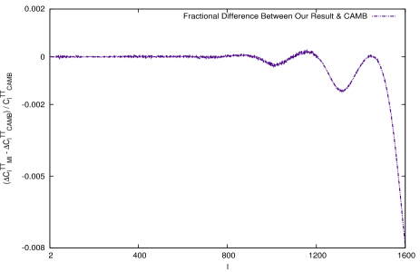
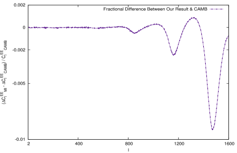
Figure 1: The fractional difference between the lensed and delensed $TT$ (left panel) and $EE$ (right panel) power spectra as obtained from our procedure compared to the corresponding difference between the lensed and unlensed spectra calculated from CAMB.

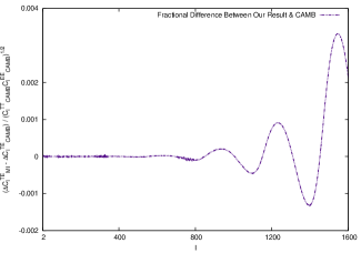
Figure 2: The fractional difference between the lensed and delensed $TE$ power spectra as obtained from our procedure compared to the corresponding difference between the lensed and unlensed spectra calculated from CAMB.

We now present results for the delensing of the WMAP7 spectra by our analysis, done in both the flat-sky approximation as well as in the spherical sky. For this, we have utilized the lensed spectra obtained from WMAP 7-year best-fit $\Lambda CDM$ + TENS data, assuming zero unlensed $B$-mode power, and delensed the spectra using the matrix inversion technique with the kernel matrices generated using the WMAP7 best-fit lensing potential. In Figs.3 and 4, we have plotted the lensing contributions as estimated from our analysis for both the flat-sky and the full-sky. For comparison, we have assumed zero intrinsic $B$-mode power. For values of $\ell\lesssim 1600$, we find that the two methods provide consistent results. The difference between the flat-sky and the full-sky results is very small in the large scale regime, and increases very slowly as we go to smaller scales, however, the fractional difference always remains less than $10^{-3}$.

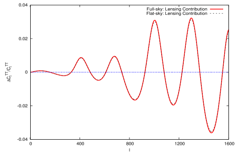
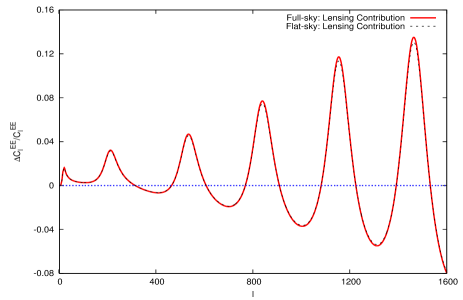
Figure 3: This shows the fractional difference between the lensed and delensed $TT$ and $EE$ power spectra as obtained by our above procedure in the flat-sky approximation (shown by black dashed lines), and in the full-sky (shown by red solid lines). The lensed spectra used are from the WMAP 7-year best-fit $\Lambda CDM$ + TENS data. Hence, the above plots describe the lensing contributions, in the flat-sky limit and in the full sky. It can be seen that the difference is very small, for this range of $\ell$-values.

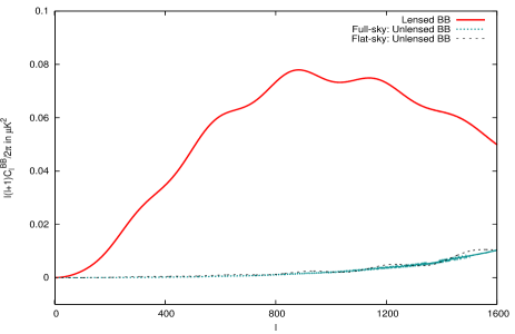
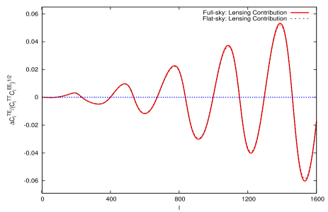
Figure 4: The left panel shows the delensed $BB$ power spectrum as obtained by our above procedure in the flat-sky approximation (black dashed line), and in the full-sky (blue dot-dashed line). The lensed $BB$ spectrum (red solid line) from the WMAP 7-year best-fit data, is also plotted to provide a comparison. The right panel shows the lensing contribution to the $TE$ power spectrum in the flat-sky approximation (black dashed lines), and in the full-sky (red solid lines). Again, it can be seen that the difference is very small, for this range of $\ell$-values.

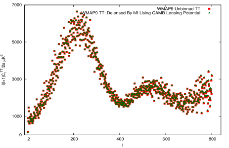
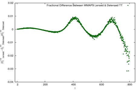
Figure 5: The left panel shows the delensed power spectrum as obtained by our above procedure in the full-sky case, using an estimate of the lensing potential power spectrum obtained from CAMB, over plotted on the WMAP 9-year unbinned $TT$ spectra. The right panel shows the fractional difference between the unbinned spectra obtained from the WMAP 9-year data and the delensed $TT$ spectra as obtained from our procedure in the full-sky case, this provides an estimate of the lensing contribution to the $TT$ power spectrum.

Let us now provide an estimate of the delensed $TT$ spectra, as obtained from our procedure using the WMAP 9-year unbinned $TT$ spectra, and an estimate of the lensing potential power spectrum obtained from CAMB using the WMAP 9-year cosmological parameters. The results are shown in Fig.5. In the left panel, the delensed spectra are over plotted on the WMAP 9-year unbinned $TT$ spectra. In the right panel, the fractional difference between the lensed and delensed spectra is plotted. It can be seen that the lensing contribution is at the level of $2-3\%$ for values of $\ell\lesssim 800$.

Finally, we furnish a brief estimate of the possible sources of error in our analysis. In the flat sky approximation, as pointed out in [Challinor & Lewis 2005], the error in ignoring terms beyond the second order in $A_{2}(\beta)$ is extremely small, of the order of $10^{-4}$. The Taylor series expansion for evaluating the unlensed spectra, Eqns. (26), (29)-(31) and Eqns.(40)-(43), ignores terms of the order of $(\delta K)^{3}$. This introduces an error of the order of $(\delta K)^{3}$, which we find to be at least four orders of magnitude below the contribution from the combination of the first and second order terms, for $\ell\lesssim 500$. As we go to higher $\ell$ values, the third order contribution increases, but it still remains at most $10^{-3}-10^{-4}$ of the first- and second-order contributions, for about $\ell\lesssim 1200$, as can be seen from Figs.6 and 7. The fractional contribution of the $(\delta K)^{3}$ term is of the order of $10^{-3}$ for the $TT$ spectrum at large multipoles $(\ell\gtrsim 1200)$, but it remains less than $10^{-4}$ for the other CMB spectra. In the full-sky analysis, we have neglected the $A_{0}(\beta)$ terms entirely as they are very small (of the order $<10^{-4}$) [Challinor & Lewis 2005]. In this case also, the contributions from the $(\delta K)^{3}$ terms are tiny, as can be seen from Figs.6 and 7. Hence, neglecting the $(\delta K)^{3}$ terms does not really incorporate significant error in our analysis. Further, our work did not take into account the effect of the non-linear evolution of the lensing potential which may also incorporate some additional error. However, non-linearities are increasingly important only in the very small scale regime. The integrated effect of the above errors leads to the overall accuracy of our analysis, estimated to be of the order of $0.33\%-0.92\%$ at the multipoles around $\ell\sim 1500$-$1600$ by the calibration technique described above. A slightly more accurate result might possibly be obtained by using the full second order expressions for the lensed correlation functions in the full sky, as provided in Appendix C of Ref. [Challinor & Lewis 2005], but would increase the computational expense.

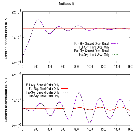
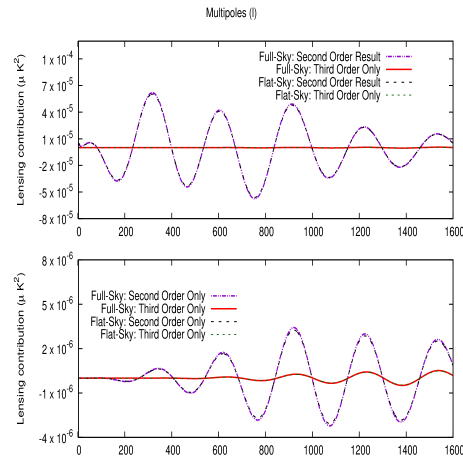
Figure 6: The left panel shows the lensing contribution to the CMB $TT$ power spectrum in units of $\mu K^{2}$. In the top half, the lensing contributions from $(\delta K)+(\delta K)^{2}$ and $(\delta K)^{3}$ are shown for both the flat-sky and the full-sky. In the bottom half, only the second- and third-order contributions are plotted, to provide an estimate of the error involved in neglecting the third order term. It is clear that the negligence of the third order kernel matrix does not incorporate any significant error in our analysis. The right panel shows the corresponding lensing contributions for the case of the $TE$ spectrum, assuming zero intrinsic $B$-mode power.

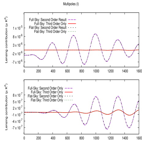
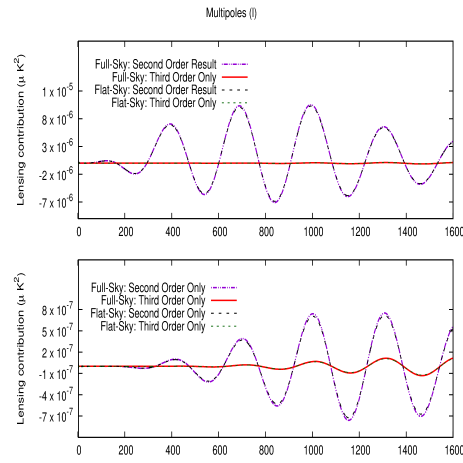
Figure 7: The left panel shows the lensing contribution to the $C^{+}$ spectrum in units of $\mu K^{2}$. In the top half, the contributions from $(\delta K)+(\delta K)^{2}$ and $(\delta K)^{3}$ are shown separately for both the flat-sky and the full-sky. In the bottom half, only the second- and third-order contributions are plotted, to provide an estimate of the error involved in neglecting the third order term. It is clear that the negligence of the third order kernel matrix does not incorporate any significant error in our analysis. The right panel shows the corresponding lensing contributions for the case of the $C^{-}$ spectrum. Here, as in the previous figure, we have assumed zero intrinsic $B$-mode power.

5 Conclusions

In this article, we have provided a new method to extract the intrinsic CMB power spectra from the lensed ones by applying a matrix inversion technique. After a through formal development of the theoretical framework, we use a FORTRAN90 code to compare our results with CAMB. We find that for $\ell\lesssim 1000$, both the results are almost identical with the fractional deviation being of the order of $10^{-4}$ or so, but as we go beyond that, the difference becomes about $0.33\%$ - $0.92\%$ around $\ell\sim 1600$. Thus, this new technique can very well serve as a first step towards direct reconstruction of intrinsic CMB power spectra from the lensed map.

To apply our methodology, the knowledge of lensing potential is necessary. The lensing potential can be reconstructed once we have the full CMB polarization data, i.e., both $E-$ and $B-$ mode. Though we do not address the lensing potential reconstruction, it may be possible to construct the CMB lensing potential from the complete polarization data alone. There is a confusion between the CMB $E$- and $B$- polarization modes due to their mixing in the presence of weak lensing. Nevertheless, using our matrix inversion technique, it may be possible to obtain a handle on the intrinsic $B$-mode power by subtracting the lensing effect due to $E$-modes, once the lensing potential is known. Of course, as we have clearly mentioned, this work is just the first step towards this reconstruction. Here, obtaining the unlensed CMB spectrum and the demonstration of deconvolution of the lensing effect has been done in the ideal situation, without taking into account noise in the measured $C_{l}$’s, uncertainties in the transfer function and in the primordial power spectrum used in the transfer function as well as errors coming from other sources as discussed in Section 4. In the realistic situation, the above uncertainties need to be incorporated. We hope to address the reconstruction of the lensing potential from the lensed CMB polarization data (with an estimate for large-scale $B$-mode power generated using CAMB) in a future work. A possible further direction in which this work may be taken is in the increase of accuracy in determining various cosmological parameters, which we hope to address in future.

References

• [Bernardeau 1997] Bernardeau, F. 1997, A&A 324, 15
• [Challinor & Chon 2002] Challinor, A. & Chon, G. 2002, PRD 66, 127301
• [Challinor & Lewis 2005] Challinor, A. & Lewis, A. 2005, PRD 71, 103010
• [Dodelson & Jubas 1993] Dodelson, S. & Jubas, J. M. 1993, PRL 70, 2224
• [Durrer 2008] Durrer, R., The Cosmic Microwave Background, Cambridge University Press, 2008
• [Hanson et al. 2013] Hanson, D. et al. 2013, arXiv:1307.5830
• [Hu 2005] Hu, W. 2005, PRD 62, 043007
• [Keisler et al. 2011] Keisler, R. et al. 2011, ApJ 743, 28
• [Kesden et al. 2002] Kesden, M., Cooray, A. & Kamionkowski, M. 2002, PRL 89, 011304
• [Knox & Song 2002] Knox, L. & Song, Y. -S. 2002, PRL 89, 011303
• [Komatsu et al. 2011] Komatsu, E. et al. 2011, ApJS 192, 18K
• [Kovak et al. 2002] Kovak, J. et al. 2002, Nature 420, 772
• [Lewis & Challinor 2006] Lewis, A. & Challinor, A. 2006, Phys. Rep. 429
• [Linder 1990] Linder, E.V. 1990, MNRAS 243, 353
• [Metcalf & Silk 1997] Metcalf, R. B. & Silk, J. 1997, ApJ 489, 1
• [Planck Collaboration 2013] Planck Collaboration, 2013, arXiv:1303.5062
• [Seljak 1995] Seljak, U. 1996, ApJ 463, 1
• [Seljak & Hirata 2004] Seljak, U. & Hirata, C. M. 2004, PRD 69, 043005
• [Smoot et al. 1992] Smoot, G. F. et al. 1992, ApJ, 396, L1
• [Swetz et al. 2011] Swetz, D. S. et al. 2011, ApJS, 194, 41
• [Zaldarriaga & Seljak 1998] Zaldarriaga, M. & Seljak, U. 1998, PRD 58, 023003