Fermion in a multi-kink-antikink soliton background,
and exotic supersymmetry

Abstract

We construct a fermion system in a multi-kink-antikink soliton background, and present in an explicit form all its trapped configurations (bound state solutions) as well as scattering states. This is achieved by exploiting an exotic $N=4$ centrally extended nonlinear supersymmetry of completely isospectral pairs of reflectionless Schrödinger systems with potentials to be $n$-soliton solutions for the Korteweg-de Vries equation. The obtained reflectionless Dirac system with a position-dependent mass is shown to possess its own exotic nonlinear supersymmetry associated with the matrix Lax-Novikov operator being a Darboux-dressed momentum. In the process, we get an algebraic recursive representation for the multi-kink-antikink backgrounds, and establish their relation to the the modified Korteweg-de Vries equation. We also indicate how the results can be related to the physics of self-consistent condensates based on the Bogoliubov-de Gennes equations.

1 Introduction and summary

Fermion systems in soliton backgrounds describe a variety of phenomena in particle, condensed matter and atomic physics. The applications include, inter alia, hadron physics, charge and fermion number fractionalization, conducting polymers, superfluidity, superconductivity, and Bose-Einstein condensation [1]–[10]. The properties of such systems are inherently related to different aspects of symmetries of the very diverse nature. Much attention to investigation of fermions in soliton backgrounds was given in the context of supersymmetry [11]–[17].

Classical solitons and quantum reflectionless systems are known to be intimately related [18, 19]. Reflectionless potentials associated with the soliton solutions to the Korteweg-de Vries (KdV) equation can be constructed, particularly, by applying Darboux-Crum transformations to a free Schrödinger particle [20]. In this picture there appear two distinct differential operators of the even and odd orders, which intertwine a reflectionless Hamiltonian supporting $n$ bound states with the Schrödinger Hamiltonian of the same $n$-soliton type [21]. Any pair of $n$-soliton Schrödinger systems can be described then by an exotic non-linear supersymmetry. This is generated not by two, as it should be expected for an ordinary supersymmetric pair of Hamiltonians, but by four higher-order differential supercharges alongside with the two bosonic integrals having the nature of the Lax-Novikov operators of the KdV hierarchy. Such exotic supersymmetry was studied by us recently in [21], where we found that its general structure, particularly the differential order of the irreducible supercharges, depends essentially on a relation between the scattering data of the partner Hamiltonian operators.

In this paper we show that within a family of completely isospectral pairs of the $n$-soliton systems, there is a peculiar subset for which two of the four supercharges are the first order matrix differential operators, while other two have the differential order $2n$. The first order supercharges are composed from differential operators intertwining the isospectral reflectionless partners directly. The supersymmetry associated with them is spontaneously broken, and the scale of the breaking is correlated with a relative shift of soliton phases of the partner potentials. Other pair of supercharges is constructed from the operators that intertwine the Hamiltonians via a virtual free particle Schrödinger system. One of the two nontrivial bosonic integrals, which are the Lax-Novikov differential operators of order $2n+1$, transmutes, in comparison with a general case of $n$-soliton paired systems, into a central charge of the nonlinear superalgebra. The condition of commutativity of the central charge with any of the two first order supercharges can be interpreted as a stationary equation of the hierarchy of the modified Korteweg-de Vries (mKdV) system represented according to the Zakharov-Shabat – Ablowitz-Kaup-Newell-Segur (ZS-AKNS) [22, 23] $2\times 2$ matrix scheme. The second nontrivial bosonic integral generates a kind of rotation between the two types of supercharges.

A remarkable possibility for alternative interpretation of one of the two first order supercharges as a Hamiltonian of a Dirac particle with a position-dependent mass provides us then with a fermion system in a multi-kink-antikink soliton background. All the scattering and bound states (trapped configurations) of the fermion system are constructed by Darboux dressing of the free massive Dirac particle. The obtained reflectionless Dirac system is shown to possess its own exotic nonlinear supersymmetry that effectively encodes its spectral peculiarities. In the process, we get a recursive representation for the multi-kink-antikink backgrounds. We also indicate how to relate the results to the physics of self-consistent condensates based on the Bogoliubov-de Gennes (BdG) equations. In this context, the multi-kink-antikink backgrounds we construct and study correspond to a generalization of the fermion-antifermion bound states solutions of Dashen, Hasslacher and Neveu [2] for the Gross-Neveu model [1]. In the last years, investigation of self-consistent solutions to the Gross-Neveu model and physics related to them experiences a renovation of interest [8, 9, 24, 25, 26, 27, 28, 29].

The paper is organized as follows. In the next section we summarize shortly the general properties of the Schrödinger $n$-soliton potentials constructed by inverse scattering method, and their relation to the KdV evolution equation and to the stationary KdV hierarchy. Then we discuss a construction of the corresponding reflectionless $n$-soliton systems from a free Schrödinger particle by means of the Darboux-Crum transformations, and show a relation of them to the non-linear Schrödinger equation. We also obtain a recursive representation for the multi-soliton potentials, and describe briefly how the exotic supersymmetric structure of a general form emerges in the extended quantum systems composed from the pairs of reflectionless $n$-soliton Schrödinger Hamiltonians. In Section 3 we prove that for any value of $n$, there is a very special $(2n+1)$-parametric $2\times 2$ matrix quantum system given by a pair of completely isospectral $n$-soliton Schrödinger partners intertwined by the first order differential operators. We also present there the explicit form of the superalgebra of the corresponding exotic $N=4$ centrally extended nonlinear supersymmetry. We reinterpret the obtained special class of supersymmetric systems in Section 4 by considering one of its two first order supercharges as a Dirac Hamiltonian. The obtained fermion system in a multi-kink-antikink background is associated then with the mKdV evolution system presented in the ZS-AKNS $2\times 2$ matrix scheme. In Section 5 the reflectionless fermion system is treated as a Darboux-dressed form of the free massive Dirac particle, and its own exotic nonlinear supersymmetry is identified. Section 6 is devoted to the concluding comments, where we discuss briefly some further interesting developments and applications of the results. We indicate, particularly, how they can be related to the physics of self-consistent condensates with both zero and nonzero values of a topological charge. In two Appendices we summarize shortly some aspects of the Dabroux and Miura transformations, which are used in the main text.

2 Reflectionless Schrödinger potentials and exotic supersymmetry

We review here briefly some properties of the soliton solutions to the KdV equation, and identify the exotic nonlinear supersymmetric structure of the extended systems composed from the reflectionless pairs of $n$-soliton Schrödinger Hamiltonians. In the process we observe a relation of the bound state eigenvalue problem for the $n$-soliton potential with the coupled system of non-linear Schrödinger equations, and obtain a recursive representation for multi-soliton potentials.

2.1 Reflectionless potentials and the KdV

There exists a variety of possible ways to construct reflectionless quantum mechanical systems. This can be done, particularly, by the inverse scattering method [19, 18], by Bäcklund [30, 31], and by Darboux-Crum [20] transformations. In the inverse scattering method, a reflectionless potential supporting $n$ bound states can be presented in a form [19, 18]

$$U_{n}(x)=-2\frac{d}{dx}K_{n}(x,x),\qquad K_{n}(x,x)=\frac{d}{dx}\ln\,[\det\mathcal{K}]\,.$$ (2.1)

Here $\mathcal{K}$ is the $n\times n$ matrix with elements

$$\mathcal{K}_{ij}=\delta_{ij}+\frac{\beta_{i}\beta_{j}}{\kappa_{i}+\kappa_{j}}\,e^{-(\kappa_{i}+\kappa_{j})x}$$ (2.2)

given in terms of $2n$ real parameters $\kappa_{j}$ and $\beta_{j}$, $j=1,\ldots,n$, $\kappa_{n}>\kappa_{n-1}>\ldots\kappa_{1}>0$, $\beta_{j}>0$. Parameters $\kappa_{j}$ correspond to the energies of the bound states, $E_{j}=-\kappa_{j}^{2}$, and $\beta_{j}$ are associated with their normalization constants. Reflectionless potential $U_{n}(x)$ satisfies an ordinary nonlinear differential equation of order $2n+1$, that is a so-called Novikov equation, or a stationary equation of the KdV hierarchy [32].

Introducing a dependence of $\beta_{j}$ on an evolution parameter $t$ in the form $\beta_{j}(t)=\beta_{j}(0)e^{4\kappa_{j}^{3}t}$, we obtain a function $U_{n}(x,t)$, which describes an $n$-soliton solution to the KdV equation [18]

$$u_{t}-6uu_{x}+u_{xxx}=0\,,$$

where $u_{t}=\frac{\partial}{\partial t}u$, $u_{x}=\frac{\partial}{\partial x}u$. For large positive and negative values of $t$, the $U_{n}(x,t)$ decouples into a linear sum of the $n$ one-soliton solutions of the amplitudes $2\kappa_{j}^{2}$, which move to the right at the speeds $v_{j}=4\kappa_{j}^{2}$,

$$U_{n}(x,t)=-\sum_{j=1}^{n}2\kappa_{j}^{2}{\rm sech}\,^{2}\kappa_{j}(x-4\kappa^{2}_{j}t\pm x^{\pm}_{0j})\,\quad{\rm as}\quad t\rightarrow\pm\infty\,.$$ (2.3)

The phases, or centers $x^{\pm}_{0j}$ of solitons are expressed in terms of the $\beta_{j}(0)$ and scaling parameters $\kappa_{j}$. At finite values of $t$, the $U_{n}(x,t)$ describes a nonlinear interaction of $n$ solitons. As a result of the soliton scattering, the phases suffer certain displacements, $x^{+}_{0j}-x^{-}_{0j}=\Delta x_{0j}(\kappa)$, which depend only on the scaling parameters [33].

A choice of $\beta_{j}(t)=\beta_{j}(0)\exp(P_{2\ell+1}(\kappa_{j})t)$ instead of $\beta_{j}(t)=\beta_{j}(0)e^{4\kappa_{j}^{3}t}$, where $P_{2\ell+1}(\kappa)$ is an odd polynomial $P_{2\ell+1}(\kappa)=a_{\ell}\kappa^{2\ell+1}+a_{\ell-1}\kappa^{2\ell-1}+\ldots+a_{1}\kappa^{3}+a_{0}\kappa$ given in terms of a set of constants $a_{0},\ldots,a_{\ell}$, generates an $n$-soliton potential which will evolve in time in accordance with some equation of the KdV hierarchy.

2.2 Darboux-Crum transformations, reflectionless potentials, and nonlinear Schrödinger equation

Another representation of the soliton systems, which is based on the Darboux transformations, is more convenient for the supersymmetric structure we are going to study. The Schrödinger Hamiltonian $H_{n}=H_{0}+U_{n}(x)$ of a reflectionless system with $n$ bound states can be obtained by applying the Darboux-Crum transformation, which is a composition of $n$ Darboux transformations, to a free particle described by $H_{0}=-\frac{d^{2}}{dx^{2}}$. A reflectionless potential in this case is represented as

$$U_{n}(x)=-2\frac{d^{2}}{dx^{2}}\ln\mathbb{W}_{n}(x)\$$ (2.4)

in terms of the Wronskian $\mathbb{W}_{n}(x)=\mathbb{W}(\psi_{1},\ldots,\psi_{n})$, $\mathbb{W}(f_{1},\ldots,f_{n})=\det W_{ij}$, $W_{ij}=\frac{d^{i-1}}{dx^{i-1}}f_{j}$, which is constructed from non-physical, exponentially divergent at infinity eigenfunctions $\psi_{j}$ of the free particle Hamiltonian, $H_{0}\psi_{j}=-\kappa_{j}^{2}\psi_{j}$,

$$\psi_{j}(x;\kappa_{j},\tau_{j})=\left\{\begin{matrix}\cosh\kappa_{j}(x+\tau_{j}),&j={\rm odd}\\ \sinh\kappa_{j}(x+\tau_{j}),&j={\rm even}\end{matrix}\,\,.\right.$$ (2.5)

The scaling parameters $\kappa_{j}$, $0<\kappa_{1}<\kappa_{2}<...<\kappa_{j-1}<\kappa_{n}$, are the same here as in (2.2), while the translation parameters $\tau_{j}$, $j=1,\ldots,n$, may take arbitrary real values, and can be related with the parameters $\beta_{j}$ in representation (2.1), (2.2). The subsets of wave functions (2.5) with even and odd values of index $j$ can be transformed mutually into each other by a complex shift of the translation parameters, $\cosh\kappa_{j}(x+\tau_{j}+i\frac{\pi}{2\kappa_{j}})=i\sinh\kappa_{j}(x+\tau_{j})$, or by a differentiation. A specific choice of the free particle Hamiltonian eigenstates in (2.5) guarantees that the Wronskian $\mathbb{W}_{n}(x)$ is a nodeless function that generates a nontrivial, $2n$-parametric non-singular potential (2.4) [21], $U_{n}=U_{n}(x;\kappa_{1},\ldots,\kappa_{n},\tau_{1},\ldots,\tau_{n}).$ The Wronskian here can be related to the determinant in representation (2.1), (2.2), $\mathbb{W}_{n}(x)=Ce^{\rho x}\det\mathcal{K}$, where $C=C(\kappa,\tau)$ and $\rho=\rho(\kappa,\tau)$ are some constants.

According to the Darboux-Crum construction, the eigenstates $\psi[n,\lambda]$ of the Schrödinger operator $H_{n}$, $H_{n}\psi[n,\lambda]=\lambda\psi[n,\lambda]$, are obtained from the free particle eigenfunctions $\psi[0,\lambda]$, $H_{0}\psi[0,\lambda]=\lambda\psi[0,\lambda]$,

$$\psi[n;\lambda]=\frac{\mathbb{W}(\psi_{1},\ldots,\psi_{n},\psi[0;\lambda])}{\mathbb{W}(\psi_{1},\ldots,\psi_{n})}\,\,.$$ (2.6)

Un-normalized physical bound states $\psi[n,-\kappa_{j}^{2}]$, $j=1,\ldots,n$, are constructed, particularly, from the non-physical free particle eigenfunctions

$$\psi[0,-\kappa_{j}^{2}](x)\equiv{\psi}^{\prime}_{j}(x;\kappa_{j},\tau_{j})=\left\{\begin{matrix}\sinh\kappa_{j}(x+\tau_{j}),&j={\rm odd}\\ \cosh\kappa_{j}(x+\tau_{j}),&j={\rm even}\end{matrix}\,.\right.$$ (2.7)

Functions (2.7) form a set complementary to (2.5), $H_{0}{\psi}^{\prime}_{j}=-\kappa_{j}^{2}{\psi}^{\prime}_{j}$. As it was noted, the set (2.7) can be related to (2.5) by a simple complex shift of translation parameters, or by a differentiation,

$${\psi}^{\prime}_{j}(x;\kappa_{j},\tau_{j})=\frac{1}{\kappa_{j}}\frac{d}{dx}\psi_{j}(x;\kappa_{j},\tau_{j})\,.$$ (2.8)

Relation (2.6) can be presented in an equivalent form

$$\psi[n;\lambda]=\mathbb{A}_{n}\psi[0;\lambda]\,,\qquad\mathbb{A}_{n}=A_{n}A_{n-1}\ldots A_{1}\,,$$ (2.9)

which will play a key role in the further analysis. Here the first order differential operators $A_{j}$ are defined recursively in terms of the functions (2.5),

$$A_{1}=\psi_{1}\frac{d}{dx}\frac{1}{\psi_{1}}=\frac{d}{dx}-(\ln\psi_{1})_{x},$$ (2.10)

$$A_{j}=(\mathbb{A}_{j-1}\psi_{j})\frac{d}{dx}\frac{1}{(\mathbb{A}_{j-1}\psi_{j})}=\frac{d}{dx}-(\ln(\mathbb{A}_{j-1}\psi_{j}))_{x}\,,\quad j=2,\ldots\,.$$ (2.11)

Indeed, the equivalence of (2.9) to (2.6) for $n=1,2$ is checked directly. Assuming that

$$\mathbb{A}_{n}\psi[0;\lambda]=\frac{\mathbb{W}(\psi_{1},\ldots,\psi_{n},\psi[0;\lambda])}{\mathbb{W}(\psi_{1},\ldots,\psi_{n})}$$ (2.12)

is valid for $n>2$, Eqs. (2.11) and (2.12) give

$$\mathbb{A}_{n+1}\psi[0;\lambda]=A_{n+1}\left(\mathbb{A}_{n}\psi[0;\lambda]\right)=(\mathbb{A}_{n}\psi_{n+1})\frac{d}{dx}\left(\frac{1}{(\mathbb{A}_{n}\psi_{n+1})}\mathbb{A}_{n}\psi[0;\lambda]\right)\,,$$ (2.13)

and

$$\mathbb{A}_{n+1}\psi[0;\lambda] = \frac{\mathbb{W}(1,\ldots,n,n+1)}{\mathbb{W}(1,\ldots,n)}\left(\frac{\mathbb{W}(1,\ldots,n)}{\mathbb{W}(1,\ldots,n,n+1)}\frac{\mathbb{W}(1,\ldots,n,0)}{\mathbb{W}(1,\ldots,n)}\right)_{x}$$ (2.14)

$$= \frac{\mathbb{W}(\mathbb{W}(1,\ldots,n,n+1),\mathbb{W}(1,\ldots,n,0))}{\mathbb{W}(1,\ldots,n)\mathbb{W}(1,\ldots,n,n+1)},$$

where $\mathbb{W}(1,\ldots,n,n+1)=\mathbb{W}(\psi_{1},\ldots,\psi_{n+1})$, $\mathbb{W}(1,\ldots,n,0)=\mathbb{W}(\psi_{1},\ldots,\psi_{n},\psi[0;\lambda])$. The Wronskian identity

$$\mathbb{W}(f_{1},\ldots,f_{n},g,h)\mathbb{W}(f_{1},\ldots,f_{n})=\mathbb{W}(\mathbb{W}(f_{1},\ldots,f_{n},g),\mathbb{W}(f_{1},\ldots,f_{n},h))\,,$$ (2.15)

which is true for any choice of the functions $f_{1},\ldots,f_{n}$, $g$ and $h$ [34], allows us to represent the fraction (2.14) in the form of the right hand side of (2.12) with $n$ changed for $n+1$. This proves the equivalence of (2.9) to (2.6) by induction.

Definition (2.11) and relation (2.12) provide also the following alternative representation for the operator $A_{n}$,

$$A_{n}=\frac{d}{dx}-\left(\ln\mathbb{A}_{n-1}\psi_{n}\right)_{x}=\frac{d}{dx}-\left(\ln\frac{\mathbb{W}_{n}}{\mathbb{W}_{n-1}}\right)_{x}\equiv\frac{d}{dx}+\mathcal{W}_{n}\,,$$ (2.16)

where

$$\mathcal{W}_{n}=\Omega_{n}-\Omega_{n-1}\,,\qquad\Omega_{n}=-(\ln\mathbb{W}_{n})_{x}\,.$$ (2.17)

Then (2.17) together with Eq. (2.4) gives one more useful representation for the $n$-soliton potential,

$$U_{n}=2\Omega_{nx}\,.$$ (2.18)

Having in mind this relation, we call $\Omega_{n}$ a pre-potential of the $n$-soliton system. Coherently with Eqs. (2.12) and (2.10), in (2.16) and (2.17) we assume $\mathbb{W}_{0}=1$, $\Omega_{0}=0$, $V_{0}=0$, and have $\mathbb{W}_{1}=\cosh\kappa_{1}(x+\tau_{1})$,

$$\Omega_{1}=-\kappa_{1}\tanh\kappa_{1}(x+\tau_{1}),\qquad U_{1}=-\frac{2\kappa_{1}^{2}}{\cosh^{2}\kappa_{1}(x+\tau_{1})}\,.$$ (2.19)

As follows from (2.11), the first order differential operator $A_{j}$ annihilates a nodeless non-physical eigenfunction $\mathbb{A}_{j-1}\psi_{j}$ of $H_{j-1}$ of eigenvalue $-\kappa_{j}^{2}$. On the other hand, $A_{j}^{\dagger}$ annihilates a function $1/(\mathbb{A}_{j-1}\psi_{j})$, which is a physical bound (ground) state of $H_{j}$ of energy $-\kappa_{j}^{2}$. This means that $U_{n}$ and $U_{n-1}$ are related by the Darboux transformation, see Appendix A. Explicitly, we have the relations

$$U_{n}=\mathcal{W}_{n}^{2}+\mathcal{W}_{nx}-\kappa_{n}^{2}\,,\qquad U_{n-1}=\mathcal{W}_{n}^{2}-\mathcal{W}_{nx}-\kappa_{n}^{2}\,,$$ (2.20)

$$A_{n}A_{n}^{\dagger}=H_{n}+\kappa_{n}^{2}\,,\qquad A_{n}^{\dagger}A_{n}=H_{n-1}+\kappa_{n}^{2}\,.$$ (2.21)

In correspondence with (2.21), the first order Darboux generators $A_{n}$ and $A_{n}^{\dagger}$ intertwine the $n$- and $(n-1)$-soliton systems,

$$A_{n}H_{n-1}=H_{n}A_{n},\qquad A_{n}^{\dagger}H_{n}=H_{n-1}A_{n}^{\dagger},$$

and relate their eigenstates,

$$\psi[n;\lambda]=A_{n}\psi[n-1;\lambda],\qquad A_{n}^{\dagger}\psi[n;\lambda]=(\lambda+\kappa_{n}^{2})\psi[n-1;\lambda],$$

cf. (2.9). The order $n$ differential operators $\mathbb{A}_{n}$ and $\mathbb{A}_{n}^{\dagger}$ intertwine, on the other hand, $H_{n}$ with a free particle Hamiltonian $H_{0}$,

$$\mathbb{A}_{n}H_{0}=H_{n}\mathbb{A}_{n},\qquad\mathbb{A}_{n}^{\dagger}H_{n}=H_{0}\mathbb{A}_{n}^{\dagger}\,.$$ (2.22)

As follows from (2.9), the free particle’s plane wave states $e^{ikx}$ are mapped into the eigenfunctions of $H_{n}$ of the form $\psi_{n}(x,k)=P_{n}(x,k)e^{ikx}$, where $P_{n}$ is a polynomial of order $n$ in $k$, $H_{n}\psi_{n}(x,k)=k^{2}\psi_{n}(x,k)$. This means that $U_{n}(x)$ is a Bargmann-Kay-Moses reflectionless potential [19], for which the transmission coefficient can be easily computed. For functions (2.5) we have $\psi_{j}(x)\sim e^{\pm\kappa_{j}(x+\tau_{j})}$ as $x\rightarrow\pm\infty$. Then we find that $A_{j}\rightarrow\frac{d}{dx}\pm\kappa_{j}$ as $x\rightarrow\mp\infty$, and in these limits $P_{n}\rightarrow P_{n\mp}=\prod_{j=1}^{n}(ik\pm\kappa_{j})$. For the transmission amplitude $t(k)=P_{n+}/P_{n-}$ this gives

$$t(k)=\prod_{j=1}^{n}\left(\frac{k+i\kappa_{j}}{k-i\kappa_{j}}\right)\,.$$ (2.23)

A class of reflectionless systems we consider turns out also to be related naturally to another completely integrable system, namely, to the nonlinear Schrödinger equation.

To see this, we first show that the reflectionless potential $U_{n}(x)$ can be presented in the form

$$U_{n}(x)=-4\sum_{j=1}^{n}\kappa_{j}\hat{\psi}^{2}_{n,j}(x)$$ (2.24)

in terms of the normalized bound states of the Hamiltonian $H_{n}$,

$$\hat{\psi}_{n,j}(x)=\mathcal{N}^{-1}_{j}\psi[n,-\kappa_{j}^{2}](x),\qquad\mathcal{N}^{2}_{j}=2\kappa_{j}\prod_{\ell=1,\,\ell\neq j}^{n}|\kappa_{\ell}^{2}-\kappa_{j}^{2}|\,,\qquad\int_{-\infty}^{+\infty}\hat{\psi}_{n,j}^{2}(x)dx=1\,,$$ (2.25)

where it is assumed that at $n=1$ the product in expression for $\mathcal{N}^{2}_{1}$ is reduced to $1$. Using relation $\frac{d}{dx}\mathbb{W}_{n}=\sum_{j=1}^{n}\mathbb{W}(\psi_{1},\ldots,\frac{d\psi_{j}}{dx},\ldots,\psi_{n})$, we can rewrite Eq. (2.4) in a form $U_{n}(x)=-2\sum_{j=1}^{n}{\mathbb{W}\left(\mathbb{W}_{n},\mathbb{W}(\psi_{1},\ldots,\frac{d\psi_{j}}{dx},\ldots,\psi_{n})\right)}/{\mathbb{W}_{n}^{2}}.$ The Wronskian identity (2.15) allows us to represent the potential equivalently as

$$U_{n}(x)=-2\sum_{j=1}^{n}\frac{\mathbb{W}(\psi_{1},\ldots,\psi_{j},\frac{d\psi_{j}}{dx},\ldots,\psi_{n})\mathbb{W}(\psi_{1},\ldots,\psi_{j-1},\psi_{j+1},\ldots,\psi_{n})}{\mathbb{W}_{n}^{2}}\,.$$ (2.26)

A relation

$$\mathbb{W}(\psi_{1},\ldots,\psi_{j},\frac{d\psi_{j}}{dx},\ldots,\psi_{n})=\frac{1}{2}\kappa_{j}\mathcal{N}_{j}^{2}\mathbb{W}(\psi_{1},\ldots,\psi_{j-1},\psi_{j+1},\ldots,\psi_{n}),$$ (2.27)

where $\mathcal{N}_{j}^{2}$ is defined in (2.25), follows from basic identities of determinants. Using this last relation together with Eqs. (2.6), (2.7) and (2.8), we rewrite (2.26) in terms of un-normalized bound states of $H_{n}$,

$$U_{n}(x)=-4\sum_{j=1}^{n}\kappa_{j}\mathcal{N}_{j}^{-2}\psi^{2}[n,-\kappa_{j}^{2}](x)\,.$$ (2.28)

Employing once more the identity (2.15) we get

$$\frac{d}{dx}\left(\frac{\mathbb{W}(\psi_{1},\ldots,\frac{d\psi_{j}}{dx},\ldots,\psi_{n})}{\mathbb{W}_{n}}\right)=$$

$$\frac{\mathbb{W}(\psi_{1},\ldots,\psi_{j-1},\psi_{j+1},\ldots,\psi_{n},\psi_{j},\frac{d\psi_{j}}{dx})\mathbb{W}(\psi_{1},\ldots,\psi_{j-1},\psi_{j+1},\ldots,\psi_{n})}{\mathbb{W}_{n}^{2}}\,.$$ (2.29)

Eq. (2.27) gives us then $\frac{d}{dx}({\mathbb{W}(\psi_{1},\ldots,\frac{d\psi_{j}}{dx},\ldots,\psi_{n})}/{\mathbb{W}_{n}})=2\kappa_{j}\mathcal{N}_{j}^{-2}\psi^{2}[n,-\kappa_{j}^{2}](x)$. Integrating this equality from $-\infty$ to $+\infty$, and using relations $\lim_{x\rightarrow\pm\infty}{\mathbb{W}(\psi_{1},\ldots,\frac{d\psi_{j}}{dx},\ldots,\psi_{n})}/{\mathbb{W}_{n}}=\pm\kappa_{j}\,,$ we reproduce (2.25), and present (2.28) in the form (2.24).

Because of relation (2.24), the equations $H_{n}\hat{\psi}_{n,j}=-\kappa_{j}^{2}\hat{\psi}_{n,j}$ for $n$ normalized bound states can be presented in a form of the system of $n$ coupled nonlinear ordinary differential equations

$$-\hat{\psi}_{n,jxx}-4\sum_{i=1}^{n}\kappa_{i}\hat{\psi}_{n,i}^{2}\hat{\psi}_{n,j}+\kappa_{j}^{2}\hat{\psi}_{n,j}=0\,.$$ (2.30)

Introduce an evolution parameter $t$, and define $q_{j}(x,t)=\exp(i\kappa_{j}^{2}t)\hat{\psi}_{n,j}(x)$. Then we find that these functions satisfy a system of $n$ coupled nonlinear Schrödinger equations,

$$iq_{jt}=-q_{jxx}-4\sum_{i=1}^{n}\kappa_{i}|q_{i}|^{2}q_{j}\,.$$ (2.31)

In the simplest case $n=1$, this reduces to a focusing case of the nonlinear Schrödinger equation,

$$iq_{t}+q_{xx}+4\kappa|q|^{2}q=0\,.$$ (2.32)

So, $n$ bound state solutions to the linear time-dependent quantum Schrödinger equation for reflectionless time-independent $n$-soliton potential provide also a solution to the system of $n$ coupled nonlinear Schrödinger equations.

2.3 Recursions for $n$-soliton pre-potentials and potentials

Here we obtain a recursion representation for $n$-soliton potentials of a general form. This will allow us in what follows to get also a recursion representation for multi-kink-antikink backgrounds, which are reflectionless Dirac potentials.

Let us take a sum of two relations in (2.20) with making use of (2.17),

$$U_{n}+U_{n-1}=2(\Omega_{n}-\Omega_{n-1})^{2}-2\kappa_{n}^{2}\,.$$ (2.33)

Changing in (2.33) $n$ for $j$, we multiply both sides of the equality by $(-1)^{n-j}$, and sum up from $j=1$ to $j=n$. As a result we obtain

$$\frac{1}{2}\,U_{n}=\Omega_{n}^{2}+\sum_{j=1}^{n}(-1)^{n-j+1}\left(2\Omega_{j}\Omega_{j-1}+\kappa_{j}^{2}\right)\,.$$ (2.34)

Assume now that the chain of reflectionless potential $U_{j}$ with $j=1\ldots,n$ is constructed by using the same chain of states (2.5) in which, however, the last two states, $\psi_{n-1}$ and $\psi_{n}$, are permuted. In such a way we get a chain of functions $\Omega_{1}(1),\ldots$, $\Omega_{n-2}(1,\ldots,n-2)$, $\Omega_{n-1}(1,\ldots,n-2,n)$, $\Omega_{n}(1,\ldots,n-2,n,n-1)$. Since $\mathbb{W}(1,\ldots,n-2,n,n-1)=-\mathbb{W}(1,\ldots,n-2,n-1,n)$, we have $\Omega_{n}(1,\ldots,n-2,n,n-1)=\Omega_{n}(1,\ldots,n-2,n-1,n)$, and in the indicated chain of pre-potentials only the penultimate term $\Omega_{n-1}(1,\ldots,n-2,n)$ is different from the corresponding term $\Omega_{n-1}(1,\ldots,n-2,n-1)$ in the initial, non permuted chain. The same is valid for corresponding chain of potentials by virtue of relation (2.18). Notice that ${\Omega}_{n-1}^{\sharp}\equiv\Omega_{n-1}(1,\ldots,n-2,n)$ and ${U}_{n-1}^{\sharp}\equiv U_{n-1}(1,\ldots,n-2,n)$ are singular functions of $x\in\mathbb{R}$. Particularly,

$$\Omega_{1}^{\sharp}=\Omega_{1}(2)=-\kappa_{2}\coth\kappa_{2}(x+\tau_{2})\,,\qquad U_{1}^{\sharp}={U}_{1}(2)=\frac{2\kappa_{2}^{2}}{\sinh^{2}\kappa_{2}(x+\tau_{2})}\,.$$ (2.35)

Let us write the analog of relation (2.34) assuming that we construct $U_{n}$ via the described chain with permuted two last states,

$$\frac{1}{2}\,U_{n}=\Omega_{n}^{2}+\sum_{j=1}^{n-2}(-1)^{n-j+1}\left(2\Omega_{j}\Omega_{j-1}+\kappa_{j}^{2}\right)+(2{\Omega}_{n-1}^{\sharp}\Omega_{n-2}+\kappa_{n}^{2})-(2\Omega_{n}{\Omega}_{n-1}^{\sharp}+\kappa_{n-1}^{2})\,.$$ (2.36)

Subtracting (2.36) from (2.34), we get the equality $2\Omega_{n}({\Omega}_{n-1}^{\sharp}-\Omega_{n-1})+2\Omega_{n-2}(\Omega_{n-1}-{\Omega}_{n-1}^{\sharp})+2(\kappa_{n-1}^{2}-\kappa_{n}^{2})=0,$ which gives a recursive relation for the pre-potentials $\Omega_{n}$,

$$\Omega_{n}=\Omega_{n-2}+\frac{\kappa_{n-1}^{2}-\kappa_{n}^{2}}{\Omega_{n-1}-{\Omega}_{n-1}^{\sharp}}\,,\qquad n\geq 2\,.$$ (2.37)

Eq. (2.37) for the first two cases $n=2,3$ gives

$$\Omega_{2}=\Omega_{2}(1,2)=\frac{\kappa_{1}^{2}-\kappa_{2}^{2}}{\Omega_{1}(1)-\Omega_{1}(2)}\,,\quad\Omega_{3}=\Omega_{3}(1,2,3)=\Omega_{1}(1)+\frac{\kappa_{2}^{2}-\kappa_{3}^{2}}{\Omega_{2}(1,2)-\Omega_{2}(1,3)}\,,$$ (2.38)

and corresponding singular pre-potentials are obtained from these by changing the last arguments, $\Omega_{2}^{\sharp}=\Omega_{2}(1,3)$, $\Omega_{3}^{\sharp}=\Omega_{3}(1,2,4)$. Reflectionless n-soliton potential $U_{n}$ with $n\geq 2$ can be calculated now recursively, by employing Eqs. (2.18), (2.19) and (2.37),

$$U_{n}=U_{n-2}+2\frac{d}{dx}\left(\frac{\kappa_{n-1}^{2}-\kappa_{n}^{2}}{\Omega_{n-1}-{\Omega}_{n-1}^{\sharp}}\right)\,,\quad n=2,\dots.$$ (2.39)

Particularly, for $n=2$ Eqs. (2.39), (2.19) and (2.35) give

$$U_{2}=-2(\kappa_{2}^{2}-\kappa_{1}^{2})\left(\frac{\kappa_{1}^{2}}{\cosh^{2}\chi_{1}}+\frac{\kappa_{2}^{2}}{\sinh^{2}\chi_{2}}\right)(\kappa_{2}\coth\chi_{2}-\kappa_{1}\tanh\chi_{1})^{-2}\,,$$ (2.40)

where $\chi_{j}=\kappa_{j}(x+\tau_{j}),$ $j=1,2$.

Relation (2.39) together with (2.37) corresponds to the recursive representation of $n$-soliton solutions of the KdV equation obtained by Wahlquist and Estabrook by employing Bäcklund transformations [30, 31].

2.4 Exotic supersymmetry of reflectionless $n$-soliton pairs

In this subsection we describe shortly an exotic $N=4$ supersymmetric structure that appears in the pairs of $n$-soliton Schrödinger systems of the most general form [21], and observe the peculiarity of the case of completely isospectral soliton partners. These results will be used then in next sections to identify within the family of isospectral $n$-soliton pairs a very special subfamily related to reflectionless Dirac systems, which correspond to a fermion in a multi-kink-antikink soliton background.

Let us consider two reflectionless systems $H_{n}$ and $\tilde{H}_{n}$ constructed by using two sets of the parameters, $(\kappa_{1},\ldots,\kappa_{n}$, $\tau_{1},\ldots,\tau_{n})$ and $(\tilde{\kappa}_{1},\ldots,\tilde{\kappa}_{n}$, $\tilde{\tau}_{1},\ldots,\tilde{\tau}_{n})$. Each of these two Hamiltonians can be related to the free particle system $H_{0}$ by the corresponding intertwining operators of order $n$, $\mathbb{A}_{n}$ and $\tilde{\mathbb{A}}_{n}$, and by the conjugate operators $\mathbb{A}_{n}^{\dagger}$ and $\tilde{\mathbb{A}}_{n}^{\dagger}$. Relations (2.22) and similar relations for $\tilde{H}_{n}$ together with the observation that $\frac{d}{dx}$ is the integral of the free particle allow us to construct the operators which intertwine the $n$-soliton reflectionless systems $H_{n}$ and $\tilde{H}_{n}$,

$$\mathbb{Y}_{n}=\mathbb{A}_{n}\tilde{\mathbb{A}}_{n}^{\dagger}\,,\qquad\mathbb{X}_{n}=\mathbb{A}_{n}\frac{d}{dx}\tilde{\mathbb{A}}_{n}^{\dagger}\,,$$ (2.41)

$$\mathbb{J}_{n}\tilde{H}_{n}=H_{n}\mathbb{J}_{n}\,,\qquad\mathbb{J}_{n}^{\dagger}H_{n}=\tilde{H}_{n}\mathbb{J}_{n}^{\dagger},\quad\text{where}\quad\mathbb{J}_{n}=\mathbb{Y}_{n}\,,\,\mathbb{X}_{n}\,.$$ (2.42)

Operator $\mathbb{Y}_{n}$ is the differential operator of the even order $2n$, while $\mathbb{X}_{n}$ is the differential operator of the odd order $2n+1$. On the other hand, differential operators of order $2n+1$,

$$\mathbb{Z}_{n}=\mathbb{A}_{n}\frac{d}{dx}\mathbb{A}_{n}^{\dagger}\,,\qquad\tilde{\mathbb{Z}}_{n}=\tilde{\mathbb{A}}_{n}\frac{d}{dx}\tilde{\mathbb{A}}_{n}^{\dagger}\,,$$ (2.43)

being the Darboux-dressed forms of the free particle integral $\frac{d}{dx}$, are the integrals for $H_{n}$ and $\tilde{H}_{n}$,

$$[\mathbb{Z}_{n},H_{n}]=0,\qquad[\tilde{\mathbb{Z}}_{n},\tilde{H}_{n}]=0.$$ (2.44)

Operator $\mathbb{Z}_{n}$ can be presented in a form $\mathbb{Z}_{n}=(-1)^{n}\frac{d^{2n+1}}{dx^{2n+1}}+\sum_{j=1}^{2n}a_{2n-j}(x)\frac{d^{2n-j}}{dx^{2n-j}}$, where coefficients $a_{2n-j}(x)$ are some functions of the potential $U_{n}$ and its derivatives $U_{nx},\ldots,$ $\frac{d^{2n-1}}{dx^{2n-1}}U_{n}$. The relation of commutativity of $\mathbb{Z}_{n}$ and $H_{n}$, $[\mathbb{Z}_{n},H_{n}]=0$, is the Novikov equation, or, equivalently, a stationary higher equation of the KdV hierarchy, that defines an algebro-geometric potential $U_{n}(x)$ [33, 35]. In correspondence with the Burchnall-Chaundy theorem [36], commuting differential operators $\mathbb{Z}_{n}$ and $H_{n}$ of the mutually prime orders $2n+1$ and $2$ satisfy identically a relation $\mathbb{Z}_{n}^{2}=P_{2n+1}(H_{n})$, where $P_{2n+1}(H_{n})=H_{n}\prod_{j=1}^{n}(H_{n}+\kappa_{j}^{2})^{2}$ is a degenerate spectral polynomial of the $n$-soliton system [21]. In correspondence with this relation, integral $\mathbb{Z}_{n}$ annihilates all the singlet physical states, which are bound states of energies $E_{j}=-\kappa_{j}^{2}$, $j=1,\ldots,n$, and the state $\psi[n;0]=\mathbb{A}_{n}1$ of zero energy being the lowest state of the continuous part of the spectrum, cf. Eq. (2.9). Other $n$ states annihilated by $\mathbb{Z}_{n}$ are the non-physical eigenstates of $H_{n}$ of energies $E_{j}=-\kappa_{j}^{2}$, which can be related to the corresponding bound states by equation of the form (A.5).

In the simplest case $n=1$, the pre-prepotential and potential are given by Eq. (2.19), and we have $\mathbb{Z}_{1}=\frac{1}{4}\mathcal{Z}_{1}+\kappa_{1}^{2}\mathcal{Z}_{0},$ where $\mathcal{Z}_{0}=\frac{d}{dx}$ and $\mathcal{Z}_{1}=-4\frac{d^{3}}{dx^{3}}+6U_{1}\frac{d}{dx}+3U_{1x}$ are the Lax operators corresponding to the first two evolutionary equations from the KdV hierarchy, $u_{t}-u_{x}=0$ and $u_{t}-6uu_{x}+u_{xxx}=0$. Relation $[\mathbb{Z}_{1},H_{1}]=0$ reduces here to the Novikov equation of the form $-\frac{1}{4}(U_{1xx}-3U_{1}^{2}-4\kappa_{1}^{2}U_{1})_{x}=0$, which is satisfied due to the equality

$$U_{1xx}-3U_{1}^{2}-4\kappa_{1}^{2}U_{1}=0\,,$$ (2.45)

valid for the one-soliton potential (2.19).

By virtue of relations (2.42) and (2.44), the composed system, described by the matrix $2\times 2$ Hamiltonian $\mathcal{H}_{n}=\text{diag}\,(H_{n}\,,\tilde{H}_{n})$, possesses six nontrivial self-adjoint integrals

$$\mathcal{S}_{n,1}=\left(\begin{array}[]{cc}0&\mathbb{X}_{n}\\ \mathbb{X}_{n}^{\dagger}&0\end{array}\right),\quad\mathcal{Q}_{n,1}=\left(\begin{array}[]{cc}0&\mathbb{Y}_{n}\\ \mathbb{Y}_{n}^{\dagger}&0\end{array}\right),\quad\mathcal{P}_{n,1}=-i\left(\begin{array}[]{cc}\mathbb{Z}_{n}&0\\ 0&\tilde{\mathbb{Z}}_{n}\end{array}\right),$$ (2.46)

and $\mathcal{S}_{n,2}=i\sigma_{3}\mathcal{S}_{n,1}$, $\mathcal{Q}_{n,2}=i\sigma_{3}\mathcal{Q}_{n,1}$, $\mathcal{P}_{n,2}=\sigma_{3}\mathcal{P}_{n,1}$. A choice of the diagonal Pauli sigma matrix $\sigma_{3}$ as the $\mathbb{Z}_{2}$-grading operator identifies integrals $\mathcal{S}_{n,a}$ and $\mathcal{Q}_{n,a}$, $a=1,2$, as the fermion operators, $\{\sigma_{3},\mathcal{S}_{n,a}\}=\{\sigma_{3},\mathcal{Q}_{n,a}\}=0$, while $\mathcal{P}_{n,a}$ are identified as the boson ones, $[\sigma_{3},\mathcal{P}_{n,a}]=0$. Together with $\mathcal{H}_{n}$ they generate a nonlinear superalgebra, in which the Hamiltonian $\mathcal{H}_{n}$ plays a role of the multiplicative central charge. The superalgebraic structure given by the anti-commutation relations of these integrals, whose explicit form can be found in [21], is insensitive to translation parameters $\tau_{j}$ and $\tilde{\tau}_{j}$. Here we only write down the explicit form of the commutation relations of the bosonic integrals with the supercharges,

$$[\mathcal{P}_{n,1},\mathcal{S}_{n,a}]=i\mathcal{H}_{n}\mathbb{P}^{-}_{n}(\mathcal{H}_{n},\kappa\,,\tilde{\kappa})\mathcal{Q}_{n,a},\qquad[\mathcal{P}_{n,1},\mathcal{Q}_{n,a}]=-i\mathbb{P}^{-}_{n}(\mathcal{H}_{n},\kappa,\tilde{\kappa})\mathcal{S}_{n,a}\,,$$ (2.47)

and the commutators for $\mathcal{P}_{n,2}$ have a similar form but with $\mathbb{P}^{-}_{n}(\mathcal{H}_{n},\kappa,\tilde{\kappa})$ changed for $\mathbb{P}^{+}_{n}(\mathcal{H}_{n},\kappa,\tilde{\kappa})$, where $\mathbb{P}^{\pm}_{n}(\mathcal{H}_{n},\kappa,\tilde{\kappa})\equiv\mathbb{P}_{n}(\mathcal{H}_{n},\kappa)\pm\mathbb{P}_{n}(\mathcal{H}_{n},\tilde{\kappa})$, and

$$\mathbb{P}_{n}(\mathcal{H}_{n},\kappa)=\prod_{j=1}^{n}(\mathcal{H}_{n}+\kappa_{j}^{2}\mathds{1})\,,$$ (2.48)

with $\mathds{1}$ to be a unit $2\times 2$ matrix. From definition of $\mathbb{P}^{\pm}_{n}$ it follows that while the $\mathbb{P}^{+}_{n}$ is always a polynomial of order $n$ in the matrix Hamiltonian $\mathcal{H}_{n}$, the $\mathbb{P}^{-}_{n}$ in a generic case is a polynomial of order $(n-1)$ in $\mathcal{H}_{n}$. Moreover, in a completely isospectral case given by the conditions $\kappa_{j}=\tilde{\kappa}_{j}$, $j=1,\ldots,n$, $\mathbb{P}^{-}_{n}$ reduces to the zero operator. This means that in such a completely isospectral case the bosonic integral $\mathcal{P}_{n,1}$ transmutes into the central charge of the nonlinear superalgebra. In the next section we show that the family of the systems $\mathcal{H}_{n}$ composed from completely isospectral pairs $H_{n}$ and $\tilde{H}_{n}$ with pairwise coinciding bound states energies $E_{j}=\tilde{E}_{j}=-\kappa^{2}_{j}$, $j=1,\ldots,n$, contains a special subset of Schrödinger supersymmetric systems in which the supercharges $\mathcal{S}_{n,a}$, $a=1,2$, of differential order $(2n+1)$ are reduced to the two supercharges to be matrix differential operators of the first order.

3 Special family of isospectral $n$-soliton systems and their exotic supersymmetry

The described intertwining operators and, as a consequence, fermionic integrals for the extended system $\mathcal{H}_{n}$ are irreducible as soon as all the discrete energy levels of the subsystem $H_{n}$ are different from those for the subsystem $\tilde{H}_{n}$, i.e. when $\kappa_{j}\neq\tilde{\kappa}_{j^{\prime}}$ for any values of $j$ and $j^{\prime}$, $j,j^{\prime}=1,\ldots,n$. As it was shown in [21], when any $r$, $0<r\leq n$, discrete energy levels of one subsystem coincide with any $r$ discrete energy levels of another subsystem, one or both of the intertwining operators (2.41) are reducible in such a way that the total order of the two basic intertwining generators reduces to $4n-2r+1$. The superalgebraic structure acquires then a dependence on the corresponding $r$ relative translation parameters. As we have just seen, the case of a complete pairwise coincidence of the discrete energy levels, $\kappa_{j}=\tilde{\kappa}_{j}$, $j=1,\ldots,n$, is detected by transformation of the bosonic integral $\mathcal{P}_{n,1}$ into the central charge of the superalgebra. It was also made an observation in [21] that within such a class of the systems, there is a special, infinite family $\mathcal{H}_{n}$, $n=1,2,\ldots$, such that the corresponding completely isospectral reflectionless partners $H_{n}$ and $\tilde{H}_{n}$ are intertwined by the first order differential operators ${X}_{n}$ and $X_{n}^{\dagger}$. The first order intertwiners $X_{n}$ and $X_{n}^{\dagger}$ replace the reducible operators $\mathbb{X}_{n}$ and $\mathbb{X}_{n}^{\dagger}$ of the odd order $2n+1$, while the intertwining generators $\mathbb{Y}_{n}$ and $\mathbb{Y}_{n}^{\dagger}$ of the even order $2n$ remain to be the same as in (2.41). More precisely, in [37, 21] it was found that the reflectionless systems $H_{1}=H_{1}(\kappa_{1},\tau_{1})$ and $\tilde{\mathcal{H}}_{1}=H_{1}(\kappa_{1},\tilde{\tau}_{1})$ can be related by the first order intertwining operators $X_{1}$ and $X_{1}^{\dagger}$,

$$X_{1}=\frac{d}{dx}+\Omega_{1}-\tilde{\Omega}_{1}+\mathcal{C}_{1}\,,$$ (3.1)

so that

$$X_{1}X_{1}^{\dagger}=H_{1}+\mathcal{C}_{1}^{2},\qquad X_{1}^{\dagger}X_{1}=\tilde{H}_{1}+\mathcal{C}_{1}^{2}\,,$$ (3.2)

where $\tilde{\Omega}_{1}=\Omega(\kappa_{1},\tilde{\tau}_{1})$ and

$$\mathcal{C}_{1}=\kappa_{1}\coth\kappa_{1}(\tau_{1}-\tilde{\tau}_{1})\,.$$ (3.3)

Similarly, for the next case of $n=2$, completely isospectral Hamiltonians $H_{2}$ and $\tilde{H}_{2}$ satisfy the relations $X_{2}X_{2}^{\dagger}=H_{1}+\mathcal{C}_{2}^{2}$ and $X_{2}^{\dagger}X_{2}=\tilde{H}_{2}+\mathcal{C}_{2}^{2}$ if $\varphi_{1}\equiv\tau_{1}-\tilde{\tau}_{1}$ is fixed in terms of $\varphi_{2}\equiv\tau_{2}-\tilde{\tau}_{2}\neq 0$ by a condition $\mathcal{C}_{1}=\mathcal{C}_{2}$, where $\mathcal{C}_{2}$ and $X_{2}$ are given by relations of the form (3.3) and (3.1) with the index $1$ changed for $2$. Based on these two special cases with $n=1$ and $n=2$, it was conjectured in [21] that such a picture with the first order intertwining generators can be generalized for the case of arbitrary $n$.

We will show now that any two completely isospectral reflectionless Hamiltonians $H_{n}$ and $\tilde{H}_{n}$ with translation parameters constrained by a condition

$$\mathcal{C}_{1}=\mathcal{C}_{2}=\ldots=\mathcal{C}_{n}=\mathcal{C}\,,$$ (3.4)

are indeed related by the first order operators $X_{n}$ and $X_{n}^{\dagger}$,

$$X_{n}=\frac{d}{dx}+\Omega_{n}-\tilde{\Omega}_{n}+\mathcal{C}\,,$$ (3.5)

$$X_{n}X_{n}^{\dagger}=H_{n}+\mathcal{C}^{2},\qquad X_{n}^{\dagger}X_{n}=\tilde{H}_{n}+\mathcal{C}^{2}\,,$$ (3.6)

$$X_{n}^{\dagger}H_{n}=\tilde{H}_{n}X_{n}^{\dagger}\,,\quad X_{n}\tilde{H}_{n}=H_{n}X_{n}\,,$$ (3.7)

where $\mathcal{C}_{j}=\kappa_{j}\coth\kappa_{j}(\tau_{j}-\tilde{\tau}_{j})$, and $\mathcal{C}$ is a real parameter restricted by inequality $\mathcal{C}^{2}>\kappa_{n}^{2}$.

To prove the validity of the statement, we first rewrite Eq. (3.3) in the form

$$\mathcal{C}_{1}=\frac{\Omega_{1}\tilde{\Omega}_{1}-\kappa_{1}^{2}}{\Omega_{1}-\tilde{\Omega}_{1}}\,$$ (3.8)

by using the elementary identity $\coth(\alpha-\beta)=(1-\tanh\alpha\tanh\beta)/(\tanh\alpha-\tanh\beta)$. The chain of constraints (3.4) can be presented equivalently as

$$\mathcal{C}_{j}=\frac{\Omega_{1}(j)\tilde{\Omega}_{1}(j)-\kappa_{j}^{2}}{\Omega_{1}(j)-\tilde{\Omega}_{1}(j)}=\mathcal{C}\,,\qquad j=1,\ldots,n\,.$$ (3.9)

Relations (3.5) and (3.6) imply two equalities

$$U_{n}+\mathcal{C}^{2} = (\Omega_{n}-\tilde{\Omega}_{n}+\mathcal{C})^{2}+(\Omega_{n}-\tilde{\Omega}_{n})_{x}\,,$$ (3.10)

$$\tilde{U}_{n}+\mathcal{C}^{2} = (\Omega_{n}-\tilde{\Omega}_{n}+\mathcal{C})^{2}-(\Omega_{n}-\tilde{\Omega}_{n})_{x}\,.$$ (3.11)

To prove (3.6) under condition (3.4) we have to demonstrate the validity of relations (3.10) and (3.11). A difference of these two relations gives $U_{n}-\tilde{U}_{n}=2(\Omega_{n}-\tilde{\Omega}_{n})_{x}$, that is true because of (2.18). Denoting $\mathcal{U}_{n}\equiv U_{n}+\tilde{U}_{n}-2[(\Omega_{n}-\tilde{\Omega}_{n}+\mathcal{C})^{2}-\mathcal{C}^{2}]$, we have to show that $\mathcal{U}_{n}=0$. For $n=1$, the equality $\mathcal{U}_{1}=0$ is checked directly by using (2.19) and (3.3). Then it is sufficient to prove that $\mathcal{U}_{n}+\mathcal{U}_{n-1}=0$ for any $n>1$. From Eq. (2.33) we have $U_{n}+U_{n-1}-2[(\Omega_{n}-\Omega_{n-1})^{2}-\kappa_{n}^{2}]=0$. Let us add this last equality to its analog obtained by changing $\tau_{j}\rightarrow\tilde{\tau}_{j}$. Subtracting the obtained left hand side expression (equal to zero) from $\mathcal{U}_{n}+\mathcal{U}_{n-1}$, we arrive finally at the equality

$$\Gamma_{n}\equiv-\kappa_{n}^{2}+(\Omega_{n}-\tilde{\Omega}_{n-1})(\tilde{\Omega}_{n}-\Omega_{n-1})-\mathcal{C}(\Omega_{n}+\Omega_{n-1}-\tilde{\Omega}_{n}-\tilde{\Omega}_{n-1})=0\,,$$ (3.12)

which has to be proved. Remembering that $\Omega_{0}=\tilde{\Omega}_{0}=0$, the validity of $\Gamma_{1}=0$ follows from (3.8). Assume that the relation $\Gamma_{n}=0$ is valid for arbitrary value of $n>1$ with any admissible set of parameters satisfying the constraint (3.4). Some algebraic manipulations with employing recursive relation (2.37) with $n\rightarrow n+1$ gives rise to the equality

$$\Gamma_{n+1}=\Gamma_{n}+\frac{\kappa_{n+1}^{2}-\kappa_{n}^{2}}{(\Omega_{n}-\Omega_{n}^{\sharp})(\tilde{\Omega}_{n}-\tilde{\Omega}_{n}^{\sharp})}\left(\Gamma_{n}-\Gamma_{n}^{\sharp}\right),$$ (3.13)

where $\Gamma_{n}^{\sharp}$ is obtained from $\Gamma_{n}$ by changing in (3.12) $\Omega_{n}$ and $\tilde{\Omega}_{n}$ for $\Omega_{n}^{\sharp}$ and $\tilde{\Omega}_{n}^{\sharp}$, and $\kappa_{n}$ for $\kappa_{n+1}$, and we have taken into account here constraint (3.4) extended for the case $n\rightarrow n+1$. The equality $\Gamma_{n+1}=0$ follows then from $\Gamma_{n}=0$, that proves the validity of relations (3.6) for completely isospectral pairs of reflectionless $n$-soliton Hamiltonians with translation parameters constrained by the condition (3.4).

Condition (3.4) allows us to fix the shifts $\varphi_{j}=\tau_{j}-\tilde{\tau}_{j}$, $j=1,\ldots,n,$ in terms of the free parameter $\mathcal{C}$, $\mathcal{C}^{2}>\kappa_{n}^{2}$, and $\kappa_{j}$,

$$\varphi_{j}(\kappa_{j},\mathcal{C})=\frac{1}{2\kappa_{j}}\ln\frac{\mathcal{C}+\kappa_{j}}{\mathcal{C}-\kappa_{j}}=\frac{1}{\kappa_{j}}\text{arctanh}(\kappa_{j}/\mathcal{C})\,.$$ (3.14)

A reflectionless system $\mathcal{H}_{n}$ from the special infinite family characterized by the properties (3.4), (3.5), (3.6) and (3.7) is given therefore by $2n+1$ parameters. Denoting

$$\Delta_{n}(x)=\Delta_{n}(x;\kappa_{j},\tau_{j},\mathcal{C})\equiv\Omega_{n}\left(\kappa_{j}(x+\tau_{j})\right)-\Omega_{n}\left(\kappa_{j}(x+\tau_{j}-\varphi_{j}(\kappa_{j},\mathcal{C}))\right)+\mathcal{C}\,,$$ (3.15)

we present the first order intertwining operator in the form

$$X_{n}(x;\kappa_{j},\tau_{j},\mathcal{C})=\frac{d}{dx}+\Delta_{n}(x;\kappa_{j},\tau_{j},\mathcal{C})\,,$$ (3.16)

that can be compared with the structure of the first order differential operator $A_{n}=\frac{d}{dx}+\Omega_{n}-\Omega_{n-1}=\frac{d}{dx}+\mathcal{W}_{n}$. In correspondence with (3.10), we have

$$\Delta_{n}^{2}+\Delta_{nx}=U_{n}+\mathcal{C}^{2}\,,\qquad\Delta_{n}^{2}-\Delta_{nx}=\tilde{U}_{n}+\mathcal{C}^{2}\,,$$ (3.17)

cf. (2.20). It is worth to note here that the change

$$\mathcal{C}\rightarrow-\mathcal{C},\qquad\tau_{j}\rightarrow\tau_{j}-\varphi_{j}(\kappa_{j},\mathcal{C})=\tilde{\tau}_{j}$$ (3.18)

induces the changes $\Delta_{n}(x)\rightarrow-\Delta_{n}(x)$, $U_{n}(x)\leftrightarrow\tilde{U}_{n}(x)$. Note also that the points $x_{*}$ where the values of potentials $U_{n}$ and $\tilde{U}_{n}$ coincide, $U_{n}=\tilde{U}_{n}$, correspond in general to local extrema of $\Delta_{n}$, see Figure 1 illustrating the cases $n=1$ and $n=2$ with $\mathcal{C}>0$.

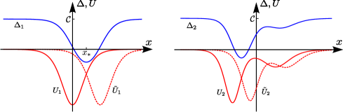
Figure 1: On the left: One-soliton isospectral potentials of the Pöschl-Teller form (2.19), and corresponding superpotential (kink-anti-kink background) $\Delta_{1}$. Relative phase $\tau_{1}-\tilde{\tau}_{1}$ coincides here with the distance between minima of potentials $\tilde{U}_{1}$ and $U_{1}$, and defines the asymptotic value $\mathcal{C}$ of the superpotential via the relation (3.3). The $\Delta_{1}(x)$ has a mirror-symmetric form, and $n=1$ is a unique case for which $\tilde{U}_{n}$ is a simple translation of $U_{n}$. On the right: Isospectral two-soliton potentials of the general form (2.40), with relative soliton phases subjected to the condition (3.4), or, equivalently, with the translation parameters shifts related by Eq. (3.14). The values of potentials coincide in three different points, where the corresponding superpotential $\Delta_{2}$ has three extrema, two of which correspond to two local minima. Note that $\Delta_{n}$ with $n>1$ not obligatorily has $n$ minima. For instance, the potential $U_{2}$ with $\kappa_{2}=2\kappa_{1}$ and $\tau_{2}=\tau_{1}$ will have a symmetric form, similar to the form (2.19) of the one-soliton Pöschl-Teller potential $U_{1}$ with the amplitude coefficient $-2\kappa_{1}^{2}$ changed for $-6\kappa_{1}^{2}$. In this case the isospectral potential $\tilde{U}_{2}$ with translation parameters given by Eq. (3.14) will have a form different from that of $U_{2}$ and will coincide with it only in one point, and corresponding superpotential (reflectionless Dirac potential, see below) $\Delta_{2}$ will have only one minimum.

The first order operators $X_{n}$, $A_{n}$ and $\tilde{A}_{n}$ satisfy the intertwining relation

$$A_{n}X_{n-1}=X_{n}\tilde{A}_{n}\,.$$ (3.19)

To show this, we note that (3.19) is equivalent to the equality

$$(\mathcal{C}+\Omega_{n-1}-\tilde{\Omega}_{n})(\Omega_{n}-\tilde{\Omega}_{n}-\Omega_{n-1}+\tilde{\Omega}_{n-1})=(\tilde{\Omega}_{n}-\Omega_{n-1})_{x}\,.$$ (3.20)

By virtue of relations $U_{n}=2\Omega_{nx}$ and (3.11), and the second equality from (2.20), we have

$$(\tilde{\Omega}_{n}-\Omega_{n-1})_{x}=(\Omega_{n-1}-\tilde{\Omega}_{n})(2\Omega_{n}-\tilde{\Omega}_{n}-\Omega_{n-1})+2\mathcal{C}(\Omega_{n}-\tilde{\Omega}_{n})+\kappa_{n}^{2}\,.$$ (3.21)

As a consequence, (3.20) is reduced to the equality $\Gamma_{n}=0$, see Eq. (3.12), that proves validity of relation (3.19). Having in mind the definition (3.6), intertwining relation $X_{n}\tilde{H}_{n}=H_{n}X_{n}$, and that $H_{n}=H_{n}(\kappa_{j},\tau_{j})$, $\tilde{H}_{n}=H_{n}(\kappa_{j},\tilde{\tau}_{j})$, it is convenient to write $X_{n}=X_{n}(\tau_{j},\tilde{\tau_{j}})$. Then $X_{n}^{\dagger}(\tau_{j},\tilde{\tau}_{j})=-X_{n}(\tilde{\tau}_{j},\tau_{j})$, and a conjugation of (3.19) after the change $\tau_{j}\leftrightarrow\tilde{\tau}_{j}$ gives us also the intertwining relation

$$X_{n-1}\tilde{A}_{n}^{\dagger}=A_{n}^{\dagger}X_{n}\,.$$ (3.22)

Using (3.19) and (3.22), we find that the intertwining operator $\mathbb{X}_{n}$ of order $2n+1$ defined in (2.41), in the present case of the special isospectral pairs of the Hamiltonians reduces as

$$\mathbb{X}_{n}=-\mathcal{C}\mathbb{Y}_{n}+\prod_{j=1}^{n}(H_{n}+\kappa_{j}^{2})\cdot X_{n}\,.$$ (3.23)

Equivalently, this can be presented in the form

$$\mathbb{A}_{n}X_{0}\tilde{\mathbb{A}}^{\dagger}_{n}=\prod_{j=1}^{n}(H_{n}+\kappa_{j}^{2})\cdot X_{n}\,,\qquad X_{0}=\frac{d}{dx}+\mathcal{C}\,.$$ (3.24)

Eq. (3.24) shows that the intertwining operator $X_{n}$ is a Darboux-dressed form of the operator $X_{0}$. The operator $X_{0}$ intertwines the Hamiltonian $H_{0}$ of the free particle with itself, $[X_{0},H_{0}]=0$.

Because of the reducible character of the operator $\mathbb{X}_{n}$, integrals $\mathcal{S}_{n,a}$ of the system $\mathcal{H}_{n}={\rm diag}\,(H_{n},\tilde{H}_{n})$ from the special family we consider are also reducible, $\mathcal{S}_{n,a}=-\mathcal{C}\mathcal{Q}_{n,a}+\prod_{j=1}^{n}(\mathcal{H}_{n}+\kappa_{j}^{2})\breve{\mathcal{S}}_{n,a}$, where $\breve{\mathcal{S}}_{n,a}$ have a structure like in (2.46) but with differential operators $\mathbb{X}_{n}$ and $\mathbb{X}_{n}^{\dagger}$ of the order $2n+1$ changed for the first order operators $X_{n}$ and $X_{n}^{\dagger}$. The nontrivial integrals $\breve{\mathcal{S}}_{n,a}$, $\mathcal{Q}_{n,a}$ and $\mathcal{P}_{n,a}$ generate together with the Hamiltonian $\mathcal{H}_{n}$ a nonlinear superalgebra with the following nontrivial (anti)-commutation relations,

$$\{\breve{\mathcal{S}}_{a},\breve{\mathcal{S}}_{b}\}=2\delta_{ab}(\mathcal{H}_{n}+\mathcal{C}^{2}),\quad\{\mathcal{Q}_{a},\mathcal{Q}_{b}\}=2\delta_{ab}\mathbb{P}_{n}^{2}\,,\quad\{\breve{\mathcal{S}}_{a},\mathcal{Q}_{b}\}=2\delta_{ab}\mathcal{C}\mathbb{P}_{n}+2\epsilon_{ab}\mathcal{P}_{1}\,,$$ (3.25)

$$[\mathcal{P}_{2},\breve{\mathcal{S}}_{a}]=2i\left((\mathcal{H}_{n}+\mathcal{C}^{2})\mathcal{Q}_{a}-\mathcal{C}\mathbb{P}_{n}\breve{\mathcal{S}}_{a}\right)\,,\quad[\mathcal{P}_{2},\mathcal{Q}_{a}]=2i\mathbb{P}_{n}\left(\mathcal{C}\mathcal{Q}_{a}-\mathbb{P}_{n}\breve{\mathcal{S}}_{a}\right)\,,$$ (3.26)

where $\mathbb{P}_{n}=\mathbb{P}_{n}(\mathcal{H}_{n},\kappa)$ is the operator defined in Eq. (2.48), and to simplify expressions, we omitted index $n$ in notation of the integrals $\breve{\mathcal{S}}_{n,a}$, $\mathcal{Q}_{n,a}$ and $\mathcal{P}_{n,a}$. Integral $\mathcal{P}_{n,1}$ commutes with all other integrals, and plays a role of the central charge of the superalgebra.

As follows from (3.25), (2.48), and relation $\mathcal{C}^{2}>\kappa_{j}^{2}$, the first order supercharges $\breve{\mathcal{S}}_{a}$ are the positive definite operators, and the part of supersymmetry associated with them is spontaneously broken. According to the first relation from (3.25), the kernels of these two supercharges are formed by non-physical eigenstates of $\mathcal{H}_{n}$. On the other hand, each of the two supercharges $\mathcal{Q}_{a}$ detects all the doubly degenerate discrete eigenvalues of $\mathcal{H}_{n}$ by annihilating all the $2n$ bound states of the matrix Hamiltonian operator. The central supercharge $\mathcal{P}_{n,1}$, generated via the anticommutation of supercharges $\breve{\mathcal{S}}_{a}$ and $\mathcal{Q}_{b}$ with $a\neq b$, annihilates not only all the bound states, but also detects two zero energy states at the edge of the continuum part of the spectrum of $\mathcal{H}_{n}$ by annihilating them. The rest of the continuous part of the spectrum of $\mathcal{H}_{n}$ with $E>0$ is the fourth-fold degenerate. The second nontrivial bosonic integral, $\mathcal{P}_{n,2}$, not appearing in the anticommutation relations of the supercharges, plays a role of the operator acting on the pairs of supercharges $(\breve{\mathcal{S}}_{a},\,\mathcal{Q}_{a})$ with $a=1$ and $a=2$ as a rotation type operator. Note that from (3.26) it follows, particularly, that $[\mathcal{P}_{2},\mathcal{C}Q_{a}-\mathbb{P}_{n}\breve{\mathcal{S}}_{a}]=-2i\mathbb{P}_{n}\mathcal{H}_{n}Q_{a}$.

4 Dirac reflectionless systems and the mKdV solitons

Let us look at the obtained results from a completely different, though related, perspective. Take one of the two integrals $\breve{\mathcal{S}}_{n,a}$, say $\breve{\mathcal{S}}_{n,1}$, and identify it as a Dirac type Hamiltonian,

$$\mathcal{H}_{n}^{D}=\left(\begin{array}[]{cc}0&X_{n}\\ X_{n}^{\dagger}&0\end{array}\right)=\left(\begin{array}[]{cc}0&\partial_{x}+\Delta_{n}\\ -\partial_{x}+\Delta_{n}&0\end{array}\right).$$ (4.1)

According to Eq. (3.24), in the case $n=0$ operator (4.1) describes a free Dirac particle of the mass $|\mathcal{C}|$, $\mathcal{H}_{0}^{D}=-i\frac{d}{dx}\sigma_{2}+\mathcal{C}\sigma_{1}$, while $\mathcal{H}_{n}^{D}$ with $n\geq 1$ is a Darboux-dressed form of $\mathcal{H}_{0}^{D}$, $\mathcal{A}_{n}\mathcal{H}_{0}^{D}\mathcal{A}_{n}^{\dagger}=\mathcal{H}_{n}^{D}\prod_{j=1}^{n}\left((\mathcal{H}^{D}_{n})^{2}+(\kappa_{j}^{2}-\mathcal{C}^{2})\mathds{1}\right)$, where $\mathcal{A}_{n}=\text{diag}\,(\mathbb{A}_{n},\tilde{\mathbb{A}}_{n})$, see Eq. (3.24). In last section it will be indicated that the first order matrix reflectionless operator $\mathcal{H}_{n}^{D}$ can also be considered as the BdG Hamiltonian in Andreev approximation [38]. Then function $\Delta_{n}(x)$ appearing in its structure has, in dependence on a physical context, a meaning of a gap function, a condensate, an order parameter, or just a position-dependent mass. Note that relations (3.16), (3.14), (2.37), (2.19) and (2.38) allow us to construct $\Delta_{n}(x)$ recursively for any $n$.

The Dirac reflectionless system (4.1) has a nontrivial matrix integral $\mathcal{P}_{n,1}$ given by Eqs. (2.46), (2.43), which is a dressed form of the linear momentum integral $-i\frac{d}{dx}\mathds{1}$ of the free Dirac particle $\mathcal{H}_{0}^{D}$, $\mathcal{P}_{n,1}=\mathcal{A}_{n}(-i\frac{d}{dx}\mathds{1})\mathcal{A}_{n}^{\dagger}$. The relation of commutativity $[\mathcal{H}^{D}_{n},\mathcal{P}_{n,1}]=0$, following immediately from the Darboux-dressed nature of the matrix operators $\mathcal{H}_{n}^{D}$ and $\mathcal{P}_{n,1}$ is equivalent to the intertwining relation

$$\mathbb{Z}_{n}X_{n}=X_{n}\tilde{\mathbb{Z}}_{n}\,,$$ (4.2)

and to the conjugate relation, $X_{n}^{\dagger}\mathbb{Z}_{n}=\tilde{\mathbb{Z}}_{n}X_{n}^{\dagger}$, which follows from (4.2) under the change $\tau_{j}\leftrightarrow\tilde{\tau}_{j}$.

Consider as an example in more detail the simplest nontrivial case $n=1$ [2]. We have

$$\Delta=\kappa\left(-\tanh\kappa(x+\tau)+\tanh\kappa(x+\tilde{\tau})\right)+\mathcal{C},\qquad\mathcal{C}=\kappa\,{\rm coth}\,\kappa(\tau-\tilde{\tau})\,,$$ (4.3)

and so, the sign of $\mathcal{C}$ coincides with the sign of $(\tau-\tilde{\tau})$. To simplify notations, we omitted here index $1$ in $\Delta$, $\kappa$ and $\tau$. This gap function satisfies an ordinary nonlinear differential equation

$$\Delta_{x}^{2}=(\Delta-\mathcal{C})^{2}(\Delta-\delta_{+})(\Delta-\delta_{-})\,,\quad{\rm where}\quad\delta_{\pm}=-\mathcal{C}\pm 2\sqrt{\mathcal{C}^{2}-\kappa^{2}}\,.$$ (4.4)

From (4.3) it follows that $\Delta(x)$ is even function with respect to the point $x=x_{*}\equiv-\frac{1}{2}(\tau+\tilde{\tau})$, where it takes a minimum (or maximum) value $\delta_{+}$ (or $\delta_{-}$) for $\mathcal{C}>0$ ($\mathcal{C}<0$). Its form for the case $\mathcal{C}>0$ is shown on Figure 1.

As a consequence of (4.4), $\Delta(x)$ satisfies also equations

$$\Delta_{xx}=2\Delta^{3}+2\Delta(2\kappa^{2}-3\mathcal{C}^{2})+4\mathcal{C}(\mathcal{C}^{2}-\kappa^{2})\,,$$ (4.5)

$$\Delta_{xxx}=6\Delta^{2}\Delta_{x}+2\Delta_{x}(2\kappa^{2}-3\mathcal{C}^{2})\,.$$ (4.6)

With taking into account relation (2.45), we find that for $n=1$ the intertwining relation (4.2) is equivalent, as a condition of equality to zero of the coefficients at $d^{2}/dx^{2}$, $d/dx$ and $1$, to the three equations: $\,U-\tilde{U}=2\Delta_{x}$, $2(U-\tilde{U})\Delta+(U_{x}-3\tilde{U}_{x})=4\Delta_{xx}$ and $(6U+4\kappa^{2})\Delta_{x}+3(U_{x}-\tilde{U}_{x})\Delta-3\tilde{U}_{xx}=4\Delta_{xxx}$. The first two of these equations are satisfied by virtue of (3.17). The third equation is then satisfied by taking into account (2.45) and relation of the same form for $\tilde{U}$.

Let us present equality (4.6) satisfied by the function $\Delta=\Delta(x;\tau,\mathcal{C})$ in the form $6\Delta^{2}\Delta_{x}-\Delta_{xxx}=(6\mathcal{C}^{2}-4\kappa^{2})\Delta_{x}$. Assume now that $\Delta$ depends additionally on an evolution parameter $t$ in such a way that $\Delta(x,t=0)=\Delta(x;\tau,\mathcal{C})$, and fix such a dependence in the form

$$\Delta(x,t)\equiv\Delta(x+(6\mathcal{C}^{2}-4\kappa^{2})t;\tau,\mathcal{C})\,.$$ (4.7)

Then $\Delta_{t}=\Delta_{x}(6\mathcal{C}^{2}-4\kappa^{2})$, and function $\Delta(x,t)$ will satisfy the mKdV equation $\Delta_{t}-6\Delta^{2}\Delta_{x}+\Delta_{xxx}=0$. Equation (4.6) in this case will be a stationary equation of the mKdV hierarchy.

The described observation can be generalized for the case of arbitrary $n$. For this we first note that if $U_{n}(x;\kappa_{j},\tau_{j})$ is a general $2n$-parametric $n$-soliton potential constructed in accordance with the inverse scattering method for $t=0$, the dependence on $t$ in correspondence with the KdV equation is obtained by the the substitution $\tau_{j}\rightarrow-4\kappa_{j}^{2}t+\tau_{j}^{0}$, where $\tau_{j}^{0}$, $j=1,\ldots,n$, are constant parameters. The KdV equation possesses Galilean symmetry: if $u(x,t)$ is a solution of the KdV equation, then $U(x,t)=u(x+6ct,t)+c$ is also solution for any value of a constant $c$. Let us make a shift $x\rightarrow x+6ct$ in both sides of two relations in (3.17), and rewrite the obtained right hand sides in equivalent forms $(U_{n}(x+6ct)+c)-c+\mathcal{C}^{2}$ and $(\tilde{U}_{n}(x+6ct)+c)-c+\mathcal{C}^{2}$. Put now $c=\mathcal{C}^{2}$ and denote $U_{n}(x+6\mathcal{C}^{2}t)+\mathcal{C}^{2}=u^{+}(x,t)$, $\tilde{U}_{n}(x+6\mathcal{C}^{2}t)+\mathcal{C}^{2}=u^{-}(x,t)$, $\Delta_{n}(x+6\mathcal{C}^{2}t)=v(x,t)$. Exploiting then a relation between the KdV and the mKdV equations, which is described in Appendix B, we conclude that the function

$$\Delta_{n}(x,t)=\Omega_{n}(\xi_{j})-\Omega_{n}(\tilde{\xi}_{j})+\mathcal{C}$$ (4.8)

where $\xi_{j}=\kappa_{j}(x+(6\mathcal{C}^{2}-4\kappa_{i}^{2})t+\tau_{j}^{0})$, $\tilde{\xi}_{j}=\xi_{j}-\kappa_{j}\varphi_{j}(\kappa_{j},\mathcal{C})$, $j=1,\ldots,n$, is the $n$-soliton solution of the mKdV equation $v_{t}-6v^{2}v_{x}+v_{xxx}=0$. In particular case $n=1$, Eq. (4.8) corresponds to (4.7).

5 Fermion system in a multi-kink-antikink background as a Darboux-dressed free massive Dirac particle

Here we show that the reflectionless Dirac system described by the first order matrix Hamiltonian (4.1), or that is the same, a fermion system in a multi-kink-anti-kink background, possesses its own exotic supersymmetry that is rooted in the peculiar supersymmetry of the associated Schrödinger system studied in Section 3. It can be understood as a dressed form of the supersymmetric structure of the free massive Dirac particle. This also will allow us to present the trapped configurations (bound states) and scattering states of our fermion system in an explicit analytic form.

Consider a free Dirac massive particle described by the Hamiltonian

$$\mathcal{H}^{D}_{0}=\left(\begin{array}[]{cc}0&\partial_{x}+\mathcal{C}\\ -\partial_{x}+\mathcal{C}&0\end{array}\right).$$ (5.1)

Its eigenfunctions and corresponding eigenvalues are

$$\Psi_{0,\pm}^{k}(x)=\left(\begin{array}[]{c}e^{ikx}\\ \pm e^{ik(x+\varphi(k,\mathcal{C}))}\end{array}\right),\qquad\mathcal{E}_{\pm}(k)=\pm\sqrt{\mathcal{C}^{2}+k^{2}}\,.$$ (5.2)

Here

$$\varphi(k,\mathcal{C})=\frac{1}{2ik}\ln\frac{\mathcal{C}-ik}{\mathcal{C}+ik}$$ (5.3)

is the function even in $k$, $\varphi(-k,\mathcal{C})=\varphi(k,\mathcal{C})$, and odd in $\mathcal{C}$, $\varphi(k,-\mathcal{C})=-\varphi(k,\mathcal{C})$, and the quantity $e^{ik\varphi(k,\mathcal{C})}=\frac{\mathcal{C}-ik}{\sqrt{\mathcal{C}^{2}+k^{2}}}$ is a pure phase, $|e^{ik\varphi(k,\mathcal{C})}|=1$. The wave numbers $+k$ and $-k$, $k>0$, correspond to the same, doubly degenerate energy value. The plane wave states (5.2) with $k>0$ and $k<0$ are distinguished by the momentum integral $-i\frac{d}{dx}\mathds{1}$. The eigenvalues $\mathcal{E}_{\pm}(0)=\pm|\mathcal{C}|$ at the edges of the upper and lower continuous bands are non-degenerate. The interval $-|\mathcal{C}|<\mathcal{E}<|\mathcal{C}|$ corresponds to the energy gap in the spectrum of the free massive Dirac particle.

Consider now the Dirac reflectionless system (4.1). The Hamiltonian $\mathcal{H}^{D}_{n}$ anticommutes with $\sigma_{3}$. Coherently with Eq. (5.2) corresponding to the $n=0$ case, this implies that if $\Psi_{\mathcal{E}}$ is an eigenstate of $\mathcal{H}^{D}_{n}$, $\mathcal{H}^{D}_{n}\Psi_{\mathcal{E}}=\mathcal{E}\Psi_{\mathcal{E}}$, then $\sigma_{3}\Psi_{\mathcal{E}}$ is an eigenstate of eigenvalue $-\mathcal{E}$.

The eigenstates from the upper and lower continuums in the spectrum of $\mathcal{H}^{D}_{n}$ are obtained by Darboux-dressing of the plane wave states (5.2) of the free particle, $\Psi_{n,\pm}^{k}(x)=\mathcal{A}_{n}\Psi_{0,\pm}^{k}(x)$, $\mathcal{H}^{D}_{n}\Psi_{n,\pm}^{k}(x)=\mathcal{E}_{\pm}(k)\Psi_{n,\pm}^{k}(x)$, where $\mathcal{A}_{n}$ is the diagonal $2\times 2$ matrix, $\mathcal{A}_{n}=\text{diag}\,(\mathbb{A}_{n},\tilde{\mathbb{A}}_{n})$. The bound states of $\mathcal{H}^{D}_{n}$ are constructed by Darboux-dressing of the appropriate non-physical eigenstates from the energy gap of $\mathcal{H}^{D}_{0}$. First, we note that function (5.3) for pure imaginary values $k=i\kappa_{j}$, $\kappa_{j}>0$, reduces to the relative soliton shifts $\varphi_{j}(\kappa_{j},\mathcal{C})$ given by Eq. (3.14). Taking linear combinations of the states of the form (5.2) with $k=+i\kappa_{j}$ and $k=-i\kappa_{j}$, $j=1,\ldots,n$, $0<\kappa_{1}<\ldots\kappa_{n-1}<\kappa_{n}<|\mathcal{C}|$, we construct the formal, non-physical eigenstates of $\mathcal{H}_{0}^{D}$ of eigenvalues $\mathcal{E}_{0,\pm}(j)=\pm\sqrt{\mathcal{C}^{2}-\kappa_{j}^{2}}$,

$$\Psi_{0,\pm}^{j}(x)=\left(\begin{array}[]{c}\cosh\kappa_{j}(x+\tau_{j})\\ \pm\cosh\kappa_{j}(x+\tilde{\tau}_{j})\end{array}\right)\,,\qquad\Psi_{0,\pm}^{j}(x)=\left(\begin{array}[]{c}\sinh\kappa_{j}(x+\tau_{j})\\ \pm\sinh\kappa_{j}(x+\tilde{\tau}_{j})\end{array}\right)\,,$$ (5.4)

$\mathcal{H}^{D}_{0}\Psi_{0,\pm}^{j}(x)=\mathcal{E}_{0,\pm}(j)\Psi_{0,\pm}^{j}(x)$, where $\tilde{\tau}_{j}=\tau_{j}-\varphi_{j}(\kappa_{j},\mathcal{C})$ . Here the first (second) set of the states has to be taken for the odd (even) values of the index $j$, cf. (2.5). The set of $2n$ functions (5.4) form a kernel of the matrix differential operator $\mathcal{A}_{n}$ of the order $n$. The un-normalized bound states of $\mathcal{H}^{D}_{n}$ are given by $\Psi_{n,\pm}^{j}(x)=\mathcal{A}_{n}\frac{1}{\kappa_{j}}\frac{d}{dx}\Psi_{0,\pm}^{j}(x)$, cf. (2.8). The normalized bound states of $\mathcal{H}^{D}_{n}$ can be expressed in terms of eigenstates of the associated supersymmetric Schrödinger pair of the systems, $\hat{\Psi}_{n,\pm}^{jT}(x)=\frac{1}{\sqrt{2}}(\hat{\psi}_{n,j}(x),\,\pm\hat{\tilde{\psi}}_{n,j}(x))$, $\mathcal{H}^{D}_{n}\hat{\Psi}_{n,\pm}^{j}=\mathcal{E}_{n,\pm}(j)\hat{\Psi}_{n,\pm}^{j}$, $\mathcal{E}_{n,\pm}(j)=\pm\sqrt{\mathcal{C}^{2}-\kappa_{j}^{2}}$, $j=1,\ldots,n$, where $\hat{\psi}_{j}(x)$ is given by Eq. (2.25), and $\hat{\tilde{\psi}}_{j}(x)$ are the corresponding eigenstates of $\tilde{H}_{n}$. The spectra for the cases $n=1$ and $n=2$ are illustrated by Figures 2 and 3.

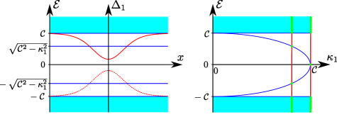
Figure 2: On the left: The form of reflectionless Dirac potential $\Delta_{1}(x)$ is shown by continuous curve for the case $\mathcal{C}>0$, while dashed curve corresponds to isospectral kink-antikink background $-\Delta_{1}(x)$ obtained by means of (3.18). Horizontal lines show two non-degenerate energy levels $\mathcal{E}=\pm\sqrt{\mathcal{C}^{2}-\kappa_{1}^{2}}$ of the bound states, and two non-degenerate energy levels $\mathcal{E}=\pm\mathcal{C}$ at the edges of the doubly degenerate continuum part of the spectrum with $\mathcal{E}>\mathcal{C}$ and $\mathcal{E}<-\mathcal{C}$. On the right: Dependence of the spectrum for reflectionless Dirac system $\mathcal{H}^{D}_{1}$ on the parameter $\kappa_{1}$. The curves correspond to the discrete energy levels $\pm\sqrt{\mathcal{C}^{2}-\kappa_{1}^{2}}$ of the bound states. Two nonzero energy levels at $0<\kappa_{1}<\mathcal{C}$ transform into one zero energy level in the limit case $\kappa_{1}=\mathcal{C}$. Kink-antikink background described by $\Delta_{1}(x)$ transforms into an antitank background $\mathcal{W}_{1}=-\kappa_{1}\tanh\kappa_{1}(x+\tau_{1})$ in the indicated limit (see also the discussion in last Section). In another limit, $\kappa_{1}\rightarrow 0$, $\mathcal{C}=const$, $\Delta_{1}(x)$ transforms into the homogeneous background $\Delta_{0}=\mathcal{C}$.

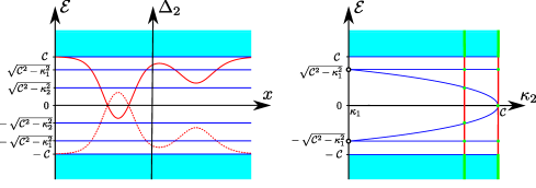
Figure 3: On the left: The form of the potential and corresponding spectrum of the reflectionless Dirac system $\mathcal{H}^{D}_{2}$ with the same notations as in Figure 2. On the right: Spectrum of reflectionless Dirac system $\mathcal{H}^{D}_{2}$ in dependence of the parameter $\kappa_{2}$ varying in the interval $\kappa_{1}<\kappa_{2}<\mathcal{C}$. In the limit case $\kappa_{2}=\kappa_{1}$, inhomogeneous reflectionless Dirac potential $\Delta_{2}$ transforms into the homogenous background $\Delta_{0}=\mathcal{C}$, see Eqs. (2.38) and (3.15), and the corresponding discrete energy levels $\pm\sqrt{\mathcal{C}^{2}-\kappa_{1}^{2}}$, shown by blank circles, disappear from the spectrum. In another limit $\kappa_{2}=\mathcal{C}$, $\mathcal{H}^{D}_{2}$ transforms into a reflectionless Dirac system with three non-degenerate energy levels, one of which has zero value. The square of $\mathcal{H}^{D}_{2}$ in this second limit gives a pair of almost isospectral reflectionless Schrödinger systems, one of which is described by a two-soliton potential supporting the bound state of zero energy, the potential of the other subsystem is one-soliton with nonzero energy of the bound state.

The nontrivial integral for the Dirac system $\mathcal{H}^{D}_{n}$ is $\mathcal{P}_{n}=\mathcal{A}_{n}(-i\frac{d}{dx}\mathds{1})\mathcal{A}_{n}^{\dagger}$, which is the central charge $\mathcal{P}_{n,1}$ of the associated reflectionless supersymmetric Schrödinger system $\mathcal{H}_{n}$. It is this operator that distinguishes the degenerate eigenstates $\Psi_{n,\pm}^{k}(x)$ with $k>0$ and $k<0$ in the continuum part of the spectrum of $\mathcal{H}^{D}_{n}$, $\mathcal{P}_{n}\Psi_{n,\pm}^{k}(x)=k\prod_{j=1}^{n}(\mathcal{E}_{n,\pm}(k)+\kappa_{j}^{2})\Psi_{n,\pm}^{k}(x)$. It also detects all the $2(n+1)$ non-degenerate eigenstates of $\mathcal{H}^{D}_{n}$ by annihilating them. The $2n$ of these states correspond to the bound states inside the energy gap between the positive and negative continuums in the spectrum of $\mathcal{H}^{D}_{n}$. The two other states are the states $\Psi_{n,\pm}^{0}(x)$ at the edges of the gap.

The trivial Lie-algebraic relation $[\mathcal{H}^{D}_{n},\mathcal{P}_{n}]=0$ does not show by itself a special nature of the higher-order matrix integral $\mathcal{P}_{n}$. This can be revealed by identification of the own supersymmetric structure of the Dirac reflectionless system $\mathcal{H}^{D}_{n}$. Consider the following operator

$$\Gamma=R_{x}\mathcal{R}_{\tau,\mathcal{C}}\sigma_{3}\,.$$ (5.5)

Here $R_{x}$ is a reflection operator for variable $x$, $R_{x}x=-xR_{x}$, $R_{x}^{2}=1$, whereas $\mathcal{R}_{\tau,\mathcal{C}}$ makes the same job for the parameters $\tau_{j}$ and $\mathcal{C}$, $\mathcal{R}_{\tau,\mathcal{C}}\tau_{j}=-\tau_{j}\mathcal{R}_{\tau,\mathcal{C}}$, $j=1,\ldots,n$, $\mathcal{R}_{\tau,\mathcal{C}}\mathcal{C}=-\mathcal{C}\mathcal{R}_{\tau,\mathcal{C}}$, $\mathcal{R}_{\tau,\mathcal{C}}^{2}=1$. Operator (5.5) commutes with the Hamiltonian $\mathcal{H}^{D}_{n}$ and anticommutes with $\mathcal{P}_{n}$, $[\Gamma,\mathcal{H}^{D}_{n}]=0$, $\{\Gamma,\mathcal{P}_{n}\}=0$. Since $\Gamma^{2}=1$, (5.5) can be treated as the $\mathbb{Z}_{2}$-grading operator, which identifies $\mathcal{H}^{D}_{n}$ and $\mathcal{P}_{n}$ as bosonic and fermionic operators, respectively. So, the reflectionless Dirac system $\mathcal{H}^{D}_{n}$ is described by its own exotic supersymmetry given by a nonlinear superalgebraic relation

$$\{\mathcal{P}_{n},\mathcal{P}_{n}\}=2\mathbb{P}^{D}_{2(n+1)}\,,\qquad\mathbb{P}^{D}_{2(n+1)}\equiv\left((\mathcal{H}^{D}_{n})^{2}-\mathcal{C}^{2}\right)\prod_{j=1}^{n}\left((\mathcal{H}^{D}_{n})^{2}+\kappa_{j}^{2}-\mathcal{C}^{2}\right)\,.$$ (5.6)

The roots of the polynomial $\mathbb{P}^{D}_{2(n+1)}(\mathcal{H}^{D}_{n})$ correspond to the $2(n+1)$ non-degenerate eigenvalues of the Hamiltonian $\mathcal{H}^{D}_{n}$. Denoting $\mathcal{P}^{D}_{n,1}=\mathcal{P}_{n}$ and defining $\mathcal{P}^{D}_{n,2}=i\Gamma\mathcal{P}^{D}_{n,1}$ as a second supercharge, a nonlinear $N=2$ superalgebra is generated for the $n$-soliton Dirac system: $\{\mathcal{P}^{D}_{n,a},\mathcal{P}^{D}_{n,b}\}=2\delta_{ab}\mathbb{P}^{D}_{2(n+1)}$, $[\mathcal{H}^{D}_{n},\mathcal{P}^{D}_{n,a}]=0$, $a,b=1,2$.

It may seem that the nature of the grading operator (5.5) is rather unusual since it includes in its structure the operator anticommuting with $\mathcal{C}$, that in the case $n=0$ is just a mass parameter. Recall that $\mathcal{C}$ can be presented in terms of the parameters $\tau_{j}$ and $\tilde{\tau}_{j}$ constrained by the relation (3.4), i.e. $\mathcal{C}=\kappa_{j}\coth\kappa_{j}(\tau_{j}-\tilde{\tau}_{j})$, $j=1,\ldots,n$. Then we see that the operator $\mathcal{R}_{\tau,\mathcal{C}}$ can alternatively be treated in a more symmetric way as the operator $\mathcal{R}_{\tau,\tilde{\tau}}$, which reflects the soliton translation parameters, $\mathcal{R}_{\tau,\tilde{\tau}}\tau_{j}=-\tau_{j}\mathcal{R}_{\tau,\tilde{\tau}}$, $\mathcal{R}_{\tau,\tilde{\tau}}\tilde{\tau}_{j}=-\tilde{\tau}_{j}\mathcal{R}_{\tau,\tilde{\tau}}$, $\mathcal{R}_{\tau,\tilde{\tau}}^{2}=1$.

6 Concluding comments and outlook

We have constructed a quantum reflectionless fermion system, which corresponds to the Dirac particle in a fixed background of a multi-kink-antikink soliton $\Delta_{n}(x)$. The $(2n+1)$-parametric function $\Delta_{n}(x)$ can be considered as an ‘instant photograph’ of a $2n$-soliton solution $v(x,t)=\Delta_{n}(x,t)$ to the mKdV equation given by Eq. (4.8). Parameter $\mathcal{C}$ corresponds here to the same nonzero asymptotic, $\Delta_{n}(x)\rightarrow\mathcal{C}\neq 0$, as $x\rightarrow-\infty$ and $x\rightarrow+\infty$, while other $2n$ parameters, $\kappa_{j}$ and $\tau_{j}$, are the scaling and translation soliton parameters. As we saw, this mKdV solution can be related to two distinct solutions $u^{+}={U}_{n}(x+6\mathcal{C}^{2}t)+\mathcal{C}^{2}$ and $u^{-}=\tilde{U}_{n}(x+6\mathcal{C}^{2}t)+\mathcal{C}^{2}$ of the KdV equation by means of relations $v^{2}\pm v_{x}=u^{\pm}$. The second order Schrödingier operators $H^{\pm}=-\frac{d^{2}}{dx^{2}}+u^{\pm}$ are factorized then in terms of the first order operators $A=\frac{d}{dx}+v$ and $A^{\dagger}=-\frac{d}{dx}+v$, $H^{+}=AA^{\dagger}$, $H^{-}=A^{\dagger}A$, which have a sense of the Darboux intertwining operators, $A^{\dagger}H^{+}=H^{-}A^{\dagger}$, $AH^{-}=H^{+}A$. In the most generic case of real nonsingular potentials $u^{+}$ and $u^{-}$, the first order scalar Darboux intertwining operators may relate either

i) a completely isospectral pair of 1D Schrödinger Hamiltonians, or

ii) almost isospectral Hamiltonians with spectra different only in one bound (ground) state.

When nonsingular $u^{+}$ and $u^{-}$ are two distinct finite-gap solutions to the KdV equation, the first possibility i) may correspond either to the case of two completely isospectral finite-gap periodic (or almost periodic) systems, or to a pair of completely isospectral $n$-soliton systems. We investigated here the soliton case with $A=X_{n}$, $H^{+}=H_{n}+\mathcal{C}^{2}$ and $H^{-}=\tilde{H}_{n}+\mathcal{C}^{2}$, which can be considered as an infinite-period limit of some isospectral pair of finite-gap periodic systems. The exotic supersymmetric structure of isospectral one-gap periodic pairs of the Schrödinger (Lamé) systems, and the corresponding Dirac particle in the kink-antikink crystal were investigated in [27] in the context of physics related to the Gross-Neveu model. It would be very interesting to generalize the analysis for the case of periodic finite-gap systems with the number of prohibited bands $n>1$.

The second possibility ii) corresponds to the situation when the quantum systems $H^{+}$ and $H^{-}$ are given by $n$- and $(n-1)$-soliton reflectionless potentials having, respectively, $n$ and $n-1$ bound states of the same energy, except the ground state of the $n$-soliton potential having in this case zero energy. In the simplest case, such a picture is realized by the pairs of reflectionless Pöschl-Teller systems [40]. The general case of almost isospectral soliton pairs given by Eqs. (2.20) and (2.21) requires a separate consideration. This, particularly, will give us a possibility to relate fermion systems in multi-kink-antikink backgrounds considered here and characterized by zero topological number, with fermion systems in the kink-type backgrounds with nonzero values of a topological charge, and to investigate exotic supersymmetric structure appearing in the extended Dirac systems. Such a generalization of the results obtained here seems to be interesting, particularly, from the perspective of their application to the physics of carbon nanostructures.

We considered the quantum mechanics of the Dirac particle in a fixed background of a multi-kink-antikink soliton. The multi-kink-antikink, as well as kink type solitons are also interesting from another perspective, related to the physics associated with the BdG equations [41, 42].

In many physical applications reflectionless potentials $\Delta(x)$ appear as stationary solutions for fermion self-consistent inhomogeneous condensates. These are given by the system of (1+1)D Dirac equations

$$\left(i\partial\!\!\!/-\Delta\right)\psi_{\alpha}=0,$$ (6.1)

subject to the constraint

$$\Delta=-g^{2}\sum_{\alpha=1}^{N}\sum_{\rm occ}\bar{\psi}_{\alpha}\psi_{\alpha}\,,$$ (6.2)

where $\sum_{\alpha=1}^{N}$ corresponds to summation in degenerate states, with $\alpha$ denoting a generalized flavour (possibly, including spin) index, and $\sum_{\rm occ}$ is a sum over the energy levels occupied by each flavour. Particularly, these equations appear in the superconductivity, in the physics of conducting polymers, and in the Gross-Neveu model [1, 2, 4, 9, 38, 43, 44].

In the context of the Bardeen-Cooper-Schrieffer theory of superconductivity, $\Delta$ corresponds to a ‘pair potential’. It is a phonon field generated by moving electrons via their interaction with ions. Dirac equation (6.1) with $N=1$ appears in the BdG method after diagonilizing the effective mean field Hamiltonian by application of Bogoliubov transformations, and by making use of the Andreev approximation, which corresponds to linearization of the non-relativistic energy dispersion near the Fermi points, or, equivalently, by neglecting second derivatives of the Bogoliubov amplitudes [45]. The so called gap equation, or self-consistency equation (6.2) for the pair potential appears in the theory from a condition of stationarity of the free energy [38]. In the physics of conducting polymers, $\Delta$ corresponds to the order parameter. The order parameter is related to the Peierls instability, which underlies the phenomenon of charge and fermion-number fractionalization [3, 4, 7]. In the Gross-Neveu model [1], being a (1+1)D toy model for strong interactions that mimics several important properties of QCD, the term $-g^{2}\sum_{\alpha=1}^{N}\bar{\psi}_{\alpha}\psi_{\alpha}$ corresponds to a nonlinear interaction of fermions with $N$ flavors. As it was demonstrated by Dashen, Hasslacher and Neveu [2], in the t’Hooft limit $N\rightarrow\infty$, with $g^{2}N$ fixed, the model can be reduced to the quasi-classical model (6.1), (6.2) [44]. Particularly, they showed that for stationary solutions, the Schrödinger potentials $V_{\pm}=\Delta^{2}\pm\Delta_{x}-\Delta_{0}^{2}$ have to be reflectionless. Their results were developed in diverse directions in [8, 9, 24, 25, 26, 27, 28, 29].

In the stationary case the Dirac equation (6.1) takes the form $(\gamma^{0}E+i\gamma^{1}\partial_{x}-\Delta)\psi(x)=0$, where we omitted the generalized flavour index $\alpha$. With the choice $\gamma^{0}=\sigma_{1}$ and $\gamma^{1}=-i\sigma_{3}$, this is reduced to the equation $\mathcal{H}_{n}^{D}\psi=E\psi$, where $\mathcal{H}_{n}^{D}$ is given by Eq. (4.1). Therefore, to relate the system we studied with the BdG system it is necessary to provide an appropriate interpretation for the consistency equation (6.2) by making use of the obtained results. We are going to present the corresponding investigation elsewhere, having also in mind a relation between condensates with zero and nonzero topological charges that has been indicated above.

Acknowledgements. The work of MSP has been partially supported by FONDECYT Grant No. 1130017, Chile. A. A. is supported by BECA DOCTORAL CONICYT 21120826. MSP is grateful to Salamanca University, where a part of this work was done, for hospitality.

Appendix A:  Darboux transformations

Here we summarize shortly the basic aspects of Darboux transformations used in the main text and in Appendix B.

Let $\psi(x)$ be an eigenstate of the second order Schrödinger operator $H=-\frac{d^{2}}{dx^{2}}+u(x)$ of eigenvalue $E$, $H\psi=E\psi$. Then

$$u-E=\phi^{2}+\phi_{x}\,,\quad\text{where}\quad\phi\equiv(\ln\psi)_{x}\,.$$ (A.1)

Define the first order differential operator $A\equiv\psi\frac{d}{dx}\frac{1}{\psi}=\frac{d}{dx}-\phi.$ By definition, $\psi$ is a kernel of $A$, $A\psi=0$, while $\frac{1}{\psi}$ is a kernel of the Hermitian conjugate operator $A^{\dagger}=-\frac{1}{\psi}\frac{d}{dx}\psi=-\frac{d}{dx}-\phi$. By Eq. (A.1), shifted for a constant Hamiltonian $H$ is factorized as

$$A^{\dagger}A=H-E\,.$$ (A.2)

Define another Hamiltonian operator $\hat{H}=-\frac{d^{2}}{dx^{2}}+\hat{u}$ by

$$AA^{\dagger}=\hat{H}-E\,,$$ (A.3)

so that $\hat{u}-E=\phi^{2}-\phi_{x}$. If potential $u(x)$ is non-singular, and eigenfunction $\psi(x)$ is nodeless, then $\hat{u}=u-2\phi_{x}$ is also a non-singular potential; otherwise it will have singularities at zeros of $\psi(x)$. Note that the function $\phi$ can be expressed in terms of the pair of potentials $u$ and $\hat{u}$ as

$$\phi=\frac{1}{2}\frac{u_{x}+\hat{u}_{x}}{u-\hat{u}}.$$ (A.4)

In accordance with (A.2) and (A.3), operators $A$ and $A^{\dagger}$ intertwine the Hamiltonians $H$ and $\hat{H}$, $AH=\hat{H}A$, $A^{\dagger}\hat{H}=HA^{\dagger}$. As a consequence, if $\psi_{\lambda}$ is an eigenstate of $H$ of eigenvalue $\lambda\neq E$, $H\psi_{\lambda}=\lambda\psi_{\lambda}$, then $A\psi_{\lambda}\equiv\hat{\psi}_{\lambda}$ is an eigenstate of $\hat{H}$ of the same eigenvalue, $\hat{H}\hat{\psi}_{\lambda}=\lambda\hat{\psi}_{\lambda}$. The operator $A^{\dagger}$ acts in the opposite direction as $A^{\dagger}\hat{\psi}_{\lambda}=(\lambda-E)\psi_{\lambda}$.

The described picture corresponds to the Darboux transformation generated by the first order differential operators $A$ and $A^{\dagger}$, which transform mutually the eigenstates of the Schrödinger operators $H$ and $\hat{H}$ with any eigenvalue $\lambda\neq E$. For eigenvalue $E$, the second, linear independent from $\psi$ solution of the Shcrödinger equation can be presented as

$$\tilde{\psi}(x)=\psi(x)\int^{x}\frac{d\xi}{\psi^{2}(\xi)}\,,$$ (A.5)

$W(\psi,\tilde{\psi})=1$. The action of the $A$ on it produces the kernel of $A^{\dagger}$, $A\tilde{\psi}\equiv\hat{\tilde{\psi}}=\frac{1}{\psi},$ $A^{\dagger}\hat{\tilde{\psi}}=0$. As a consequence, $H\tilde{\psi}=(A^{\dagger}A+E)\tilde{\psi}=E\tilde{\psi}$, and, on the other hand, $\hat{H}\hat{\tilde{\psi}}=(AA^{\dagger}+E)\hat{\tilde{\psi}}=E\hat{\tilde{\psi}}.$ Analogously, the second eigenstate of $\hat{H}$ of the eigenvalue $E$ is

$$\tilde{\hat{\tilde{\psi}}}(x)=\frac{1}{\psi(x)}\int^{x}\psi^{2}(\xi)d\xi\,.$$ (A.6)

The application of $A^{\dagger}$ to it produces the kernel of $A$, $A^{\dagger}\tilde{\hat{\tilde{\psi}}}=-\psi$.

Appendix B:  KdV and mKdV equations, and Miura transformation

Here we describe shortly the relation between the KdV equation

$$u_{t}-6uu_{x}+u_{xxx}=0,$$ (B.1)

and the modified KdV equation (mKdV)

$$v_{t}-6v^{2}v_{x}+v_{xxx}=0.$$ (B.2)

Given a function $v=v(x,t)$, let us define another function $u^{+}=u^{+}(x,t)$ by

$$u^{+}=v^{2}+v_{x}.$$ (B.3)

Assume that $v=v(x,t)$ satisfies the mKdV equation (B.2). Then $u^{+}_{t}=(2v+\partial_{x})(6v^{2}v_{x}-v_{xxx})$ and $-6u^{+}u^{+}_{x}+u^{+}_{xxx}=-(2v+\partial_{x})(6v^{2}v_{x}-v_{xxx})$, and so function (B.3) defined in terms of some solution of the mKdV equation satisfies automatically the KdV equation.

The mKdV equation (B.2) is invariant under the change $v\rightarrow-v$, while (B.3) transforms into

$$u^{-}=v^{2}-v_{x}.$$ (B.4)

Therefore, function $u^{-}$ defined by (B.4) in terms of a solution of the mKdV equation also satisfies the KdV equation.

Consider now relations (B.3) and (B.4) from another perspective. Let us assume that we are given a function $u^{+}(x,t)$, and treat relation (B.3) as a nonlinear Riccati equation that defines function $v$. If we assume that $u^{+}=u^{+}(x,t)$ satisfies the KdV equation (B.1), then we find that the function $v(x,t)$ defined by (B.3) satisfies not the mKdV, but the equation

$$(2v+\partial_{x})(v_{t}-6v^{2}v_{x}+v_{xxx})=0.$$ (B.5)

From the latter it follows a relation $v_{t}-6v^{2}v_{x}+v_{xxx}=C(t)\exp(-2\int^{x}v(\xi,t)d\xi)$, where $C(t)$ is an arbitrary function. This is reduced to the mKdV equation only in a particular case of $C(t)=0$. In the described interpretation, relation (B.3) corresponds to the Miura transformation $u^{+}\rightarrow v$ [46], which can be compared with Eq. (A.1).

If instead of (B.3) we define a function $v$ by (B.4), and assume that $u^{-}(x,t)$ satisfies the KdV equation, then instead of (B.5) we obtain the equation

$$(2v-\partial_{x})(v_{t}-6v^{2}v_{x}+v_{xxx})=0.$$ (B.6)

For each of the two Miura transformations, (B.3) or (B.4), a KdV solution generates a function $v$ which satisfies not the mKdV equation, but the equation of a more general form, (B.5) or (B.6).

Let us assume now that we have two different functions $u^{+}=u^{+}(x,t)$ and $u^{-}=u_{-}(x,t)$ given by (B.3) and (B.4) in terms of one function $v(x,t)$, and suppose that both functions $u^{+}$ and $u^{-}$ satisfy the KdV equation. In this case function $v(x,t)$ has to satisfy simultaneously the two equations (B.5) and (B.6). Adding these equations, we obtain $4v(v_{t}-6v^{2}v_{x}+v_{xxx})=0$, that implies that $v$ has to satisfy the mKdV equation (B.2). Note that in this case the solution of the mKdV equation can be expressed in terms of solutions $u^{+}$ and $u^{-}$ of the KdV equation as $v=\frac{1}{2}\frac{u^{+}_{x}+u^{-}_{x}}{u^{+}-u^{-}},$ cf. (A.4).

We conclude therefore, that if two different solutions $u^{+}$ and $u^{-}$ of the KdV equation can be expressed by means of relations (B.3) and (B.4) in terms of one function $v$, the latter ought to be a solution of the mKdV equation.

References

- [1] D. J. Gross and A. Neveu, “ Dynamical Symmetry Breaking in Asymptotically Free Field Theories,” Phys. Rev. D 10, 3235 (1974).
- [2] R. F. Dashen, B. Hasslacher and A. Neveu, “Semiclassical Bound States in an Asymptotically Free Theory,” Phys. Rev. D 12, 2443 (1975).
- [3] R. Jackiw and C. Rebbi, “ Solitons with Fermion Number 1/2,” Phys. Rev. D 13, 3398 (1976); R. Jackiw and J. R. Schrieffer, “Solitons with Fermion Number 1/2 in Condensed Matter and Relativistic Field Theories,” Nucl. Phys. B 190, 253 (1981).
- [4] W. P. Su, J. R. Schrieffer and A. J. Heeger, “ Solitons in polyacetylene,” Phys. Rev. Lett. 42, 1698 (1979); A. J. Heeger, S. Kivelson, J. R. Schrieffer and W. -P. Su, “ Solitons in conducting polymers,” Rev. Mod. Phys. 60, 781 (1988).
- [5] J. Goldstone and F. Wilczek, “Fractional Quantum Numbers on Solitons,” Phys. Rev. Lett. 47, 986 (1981).
- [6] T. L. Ho, J. R. Fulco, J. R. Schrieffer and F. Wilczek, “Solitons in Superfluid He-3-A: Bound States on Domain Walls,” Phys. Rev. Lett. 52, 1524 (1984).
- [7] A. J. Niemi and G. W. Semenoff, “Fermion Number Fractionization in Quantum Field Theory,” Phys. Rept. 135, 99 (1986); G. W. Semenoff and P. Sodano, “Stretching the electron as far as it will go,” Electron. J. Theor. Phys. 3, 157 (2006) [cond-mat/0605147].
- [8] J. Feinberg, “ On kinks in the Gross-Neveu model,” Phys. Rev. D 51, 4503 (1995) [hep-th/9408120]; “ All about the static fermion bags in the Gross-Neveu model,” Annals Phys. 309, 166 (2004) [hep-th/0305240];
- [9] M. Thies, “ From relativistic quantum fields to condensed matter and back again: Updating the Gross-Neveu phase diagram,” J. Phys. A 39, 12707 (2006) [hep-th/0601049].
- [10] T. Yefsah, A. T. Sommer, M. J.H. Ku, L. W. Cheuk, W. Ji, W. S. Bakr, and M. W. Zwierlein, “Heavy Solitons in a Fermionic Superfluid,” Nature 499, 426 (2013).
- [11] E. Witten and D. I. Olive, Supersymmetry Algebras That Include Topological Charges,” Phys. Lett. B 78, 97 (1978).
- [12] E. Witten, “Dynamical breaking of supersymmetry,” Nucl. Phys. B 188, 513 (1981); “Constraints on supersymmetry breaking,” Nucl. Phys. B 202, 253 (1982).
- [13] F. Cooper, A. Khare and U. Sukhatme, “Supersymmetry and quantum mechanics,” Phys. Rept. 251, 267 (1995) [hep-th/9405029].
- [14] J. R. Morris and D. Bazeia, “Supersymmetry breaking and Fermi balls,” Phys. Rev. D 54, 5217 (1996) [hep-ph/9607396].
- [15] G. R. Dvali and M. A. Shifman, “Domain walls in strongly coupled theories,” Phys. Lett. B 396, 64 (1997) [Erratum-ibid. B 407, 452 (1997)] [hep-th/9612128].
- [16] M. A. Shifman, A. I. Vainshtein and M. B. Voloshin, “Anomaly and quantum corrections to solitons in two-dimensional theories with minimal supersymmetry,” Phys. Rev. D 59, 045016 (1999) [hep-th/9810068].
- [17] Y. Brihaye and T. Delsate, “ Remarks on bell-shaped lumps: Stability and fermionic modes,” Phys. Rev. D 78, 025014 (2008) [arXiv:0803.1458 [hep-th]].
- [18] C. S. Gardner, J. Greene, M. Kruskal, and R. Miura, “ Method for solving the Korteweg-de Vries equation,” Phys. Rev. Lett. 19, 1095 (1967).
- [19] I. Kay and H. E. Moses, “Reflectionless Transmission through Dielectrics and Scattering Potentials,” J. Appl. Phys. 27, 1503 (1956).
- [20] V. B. Matveev and M. A. Salle, Darboux Transformations and Solitons (Springer, Berlin, 1991).
- [21] A. Arancibia, J. M. Guilarte and M. S. Plyushchay, “Effect of scalings and translations on the supersymmetric quantum mechanical structure of soliton systems,” Phys. Rev. D 87, 045009 (2013) [arXiv:1210.3666 [math-ph]].
- [22] V. E. Zakharov and A. B. Shabat, “ Exact theory of two-dimensional self-focusing and one-dimensional self-modulation of waves in nonlinear media,” Zh. Eksp. Teor. Fiz. 61, 118 (1971) [Sov. Phys. JETP 34, 62 (1972)].
- [23] M. J. Ablowitz, D. J. Kaup, A. C. Newell and H. Segur, “Nonlinear-Evolution Equations of Physical Significance,” Phys. Rev. Lett. 31, 125 (1973); “The Inverse scattering transform fourier analysis for nonlinear problems,” Stud. Appl. Math. 53, 249 (1974).
- [24] V. Schon and M. Thies, “ Emergence of Skyrme crystal in Gross-Neveu and ’t Hooft models at finite density,” Phys. Rev. D 62, 096002 (2000) [hep-th/0003195].
- [25] J. Feinberg and S. Hillel, “ Stable fermion bag solitons in the massive Gross-Neveu model: Inverse scattering analysis,” Phys. Rev. D 72, 105009 (2005) [hep-th/0509019].
- [26] G. Basar and G. V. Dunne, “ Self-consistent crystalline condensate in chiral Gross-Neveu and Bogoliubov-de Gennes systems,” Phys. Rev. Lett. 100, 200404 (2008) [arXiv:0803.1501 [hep-th]]; “Gross-Neveu Models, Nonlinear Dirac Equations, Surfaces and Strings,” JHEP 1101, 127 (2011) [arXiv:1011.3835 [hep-th]]; G. Basar, G. V. Dunne and M. Thies, “Inhomogeneous Condensates in the Thermodynamics of the Chiral NJL(2) model,” Phys. Rev. D 79, 105012 (2009) [arXiv:0903.1868 [hep-th]].
- [27] M. S. Plyushchay, A. Arancibia and L. -M. Nieto, “Exotic supersymmetry of the kink-antikink crystal, and the infinite period limit,” Phys. Rev. D 83, 065025 (2011) [arXiv:1012.4529 [hep-th]].
- [28] D. A. Takahashi and M. Nitta, “Self-consistent multiple complex-kink solutions in Bogoliubov-de Gennes and chiral Gross-Neveu systems,” Phys. Rev. Lett. 110, 131601 (2013) [arXiv:1209.6206 [cond-mat.supr-con]].
- [29] G. V. Dunne and M. Thies, “Time-Dependent Hartree-Fock Solution of Gross-Neveu models: Twisted Kink Constituents of Baryons and Breathers,” arXiv:1306.4007 [hep-th]; “Transparent Dirac potentials in one dimension: the time-dependent case,” arXiv:1308.5801 [hep-th].
- [30] H. D. Wahlquist and F.B. Estabrook, “Bäcklund Transformations for Solution of the Korteweg-de Vries Equation,” Phys. Rev. Lett. 31, 1386 (1973).
- [31] P. Drazin and R. Johnson, Solitons: An Introduction (Cambridge University Press, Cambridge, England, 1996).
- [32] S. P. Novikov, “The periodic problem for the Korteweg-de Vries equation,” Funct. Anal. Appl. 8, 236 (1975).
- [33] S. P. Novikov, S.V. Manakov, L. P. Pitaevskii, and V. E. Zakharov, Theory of Solitons (Plenum, New York, 1984).
- [34] M. M. Crum, “Associated Sturm-Liouville systems,” Quart. J. Math. Oxford Ser. (2) 6, 121 (1955), arXiv:physics/9908019.
- [35] E. D. Belokolos, A. I. Bobenko, V. Z. Enol’skii, A. R. Its, V. B. Matveev, Algebro-Geometric Approach to Nonlinear Integrable Equations (Springer, Berlin, 1994).
- [36] J. L. Burchnall and T. W. Chaundy, “Commutative Ordinary Differential Operators,” Proc. London Math. Soc. Ser. 2, s2-21, 420 (1923); Proc. Royal Soc. London. Ser. A 118, 557 (1928); I. M. Krichever, “Commutative rings of ordinary linear differential operators,” Funct. Anal. Appl. 12, 175 (1978).
- [37] M. S. Plyushchay and L. -M. Nieto, “Self-isospectrality, mirror symmetry, and exotic nonlinear supersymmetry,” Phys. Rev. D 82, 065022 (2010) [arXiv:1007.1962 [hep-th]].
- [38] I. Kosztin, S. Kos, M. Stone, and A. J. Leggett, “ Free energy of an inhomogeneous superconductor: A wave-function approach,” Phys. Rev. B 58, 9365 (1998); S. Kos and M. Stone, “Gradient expansion for the free energy of a clean superconductor,” Phys. Rev. B 59, 9545 (1999).
- [39] M. S. Plyushchay, “Deformed Heisenberg algebra, fractional spin fields and supersymmetry without fermions,” Annals Phys. 245, 339 (1996) [hep-th/9601116]; “Hidden nonlinear supersymmetries in pure parabosonic systems,” Int. J. Mod. Phys. A 15, 3679 (2000) [hep-th/9903130]; V. Jakubsky, L. -M. Nieto and M. S. Plyushchay, “The origin of the hidden supersymmetry,” Phys. Lett. B 692, 51 (2010) [arXiv:1004.5489 [hep-th]].
- [40] F. Correa, V. Jakubsky, L. -M. Nieto and M. S. Plyushchay, “Self-isospectrality, special supersymmetry, and their effect on the band structure,” Phys. Rev. Lett. 101, 030403 (2008) [arXiv:0801.1671 [hep-th]]; F. Correa, V. Jakubsky and M. S. Plyushchay, “Finite-gap systems, tri-supersymmetry and self-isospectrality,” J. Phys. A 41, 485303 (2008) [arXiv:0806.1614 [hep-th]]; “Aharonov-Bohm effect on AdS(2) and nonlinear supersymmetry of reflectionless Poschl-Teller system,” Annals Phys. 324, 1078 (2009) [arXiv:0809.2854 [hep-th]].
- [41] N. N. Bogoliubov, “A New method in the theory of superconductivity. I,” Sov. Phys. JETP 7, 41 (1958) [Zh. Eksp. Teor. Fiz. 34, 58 (1958)] [Front. Phys. 6, 399 (1961)].
- [42] P. G. de Gennes, Superconductivity of Metals and Alloys (Addison-Wesley, Redwood City, CA, 1989).
- [43] J. Bar-Sagi and C. G. Kuper, “Self-Consistent Pair Potential in an Inhomogeneous Superconductor,” Phys. Rev. Lett. 28, 1556 (1972); “ Self-consistent pair potential in superconductors. I. The superconductor-insulator boundary near ,” J. Low Temp. Phys. 16, 73 (1974).
- [44] A. Neveu and N. Papanicolaou, “ Integrability of the Classical Scalar and Symmetric Scalar-Pseudoscalar Contact Fermi Interactions in Two-Dimensions,” Commun. Math. Phys. 58, 31 (1978).
- [45] A. F. Andreev, “Thermal conductivity of the intermediate state of superconductors,” Zh. Eksp. Teor. Fiz. 46, 1823 (1964) [JETP 19, 1228 (1964)]; J. Bardeen, R. Kümmel, A. E. Jacobs, and L. Tewordt, “Structure of Vortex Lines in Pure Superconductors,” Phys. Rev. 187, 556 (1969).
- [46] R. M. Miura, “Korteweg-deVries equation and generalizations. I. A remarkable explicit nonlinear transformation,” J . Math. Phys. 9, 1202 (1968).