Overlapping Domain Decomposition Methods
for Linear Inverse Problems

Abstract

We shall derive and propose several efficient overlapping domain decomposition methods for solving some typical linear inverse problems, including the identification of the flux, the source strength and the initial temperature in second order elliptic and parabolic systems. The methods are iterative, and computationally very efficient: only local forward and adjoint problems need to be solved in each subdomain, and the local minimizations have explicit solutions. Numerical experiments are provided to demonstrate the robustness and efficiency of the methods, in particular, the convergences seem nearly optimal, i.e., they do not deteriorate or deteriorate only slightly when the mesh size reduces.

Key Words. Inverse problems, parameter identification, domain decomposition, explicit subdomain solver.

MSC 2010. 31A25, 65M55, 90C25.

1 Introduction

Domain decomposition methods (DDMs) have been developed and proved to be one of the most successful methodologies in the construction of efficient numerical solvers for solving many boundary value and initial-boundary value problems, the so-called direct problems; see [11] [13] [14] and the references therein. DDMs usually possess two important features for solving a wide class of large-scale direct problems: first, they are natural parallel solvers and can be easily implemented in parallel computers; second, their convergence may be made nearly optimal in the sense that the resulting convergence rate is nearly independent of the mesh size.

However, no much progress has been made in the construction of efficient DDMs for solving mathematically ill-posed inverse problems, although the inverse problems are usually much more challenging and time consuming than their corresponding direct problems. In [5] [10], DDMs were used indirectly for an elliptic identification problem, where classical iterative optimization algorithms were first applied for the stabilized minimization system of the identification problem, then the existing DDMs were introduced for solving the direct problems and their adjoint systems involved at each iteration. As the outer global iterations of these methods are based on the classical nonlinear optimization algorithms, their convergences deteriorate rapidly as the degrees of freedom of the entire optimization systems increase. Newton’s method was first used in [3] for solving the optimality system of the stabilized minimization of an elliptic identification problem, then an additive Schwarz type preconditioned algorithm was applied to solve the linear system involved at each Newton’s iteration. As Newton’s method requires the evaluations of the Hessian of the corresponding objective functional, the approach of [3] is applicable only to a very special formulation of the parameter identification problem. In this work we shall develop some DDMs for directly solving the stabilized minimization systems of some typical linear inverse problems so that their convergences do not deteriorate or deteriorate only mildly as the entire degrees of freedom of the optimization system grow. Next, we shall briefly address some major difficulties in the construction of DDMs for inverse problems directly, then point out the new contributions of this work.

We shall use $q$ and $u(q)$ to represent respectively the parameter function to be identified and the solution to the forward model system associated with the parameter $q$, then one may formulate a general inverse problem formally as the following forward operator equation

$$u(q)=z^{\delta}$$

where $z^{\delta}$ is the measured data of the exact solution $u$ in some subregion inside the physical domain or on part of the boundary, or at the terminal time $t=T$ when the problem is time-dependent. And the parameter $\delta$ is used here to emphasize the existence of the noise in the measured data.

Inverse problems are usually ill-posed as at least one of the following three conditions is violated: the existence, uniqueness and stability of solutions [1][2][7]. Of the three conditions stability is the most frequently encountered difficulty in numerical solutions of inverse problems. One of the most stable and effective approaches to solve general ill-posed inverse problems is to transform them into stabilized output least-squares minimizations with some appropriately selected Tikhonov regularizations, namely to minimize the following type of functionals over some constrained set $K$:

$$J(q)=\|u(q)-z^{\delta}\|^{2}_{V}+\beta N(q)$$ (1.1)

where $V$ is a Hilbert or Banach space over the measurement subregion and is determined based on the type of measurement data available, $N(q)$ is the regularization term and $\beta$ is a regularization parameter to balance between the data fitting and regularization.

One of the major difficulties in the construction of DDMs for solving a nonlinear minimization problem associated with $J(q)$ lies in the global dependence of the forward operator $u(q)$ on the parameter $q$: a change of $q$ in a small subregion of the global domain $\Omega$ causes the change of $u$ in the entire $\Omega$. This is generally true no matter if $u(q)$ is linear or nonlinear. Due to this global dependence, a direct application of the DDM principle to solve the nonlinear minimization problem of $J(q)$ may not work. To illustrate this point more clearly, we consider a decomposition of the global minimization of $J(q)$ over the entire domain $\Omega$ into a set of subproblems that involve only all sub-minimizations of functionals $J_{i}(q_{i}+\tilde{q})$ on the subdomains $\Omega_{i}$, where $q_{i}$ has support only in $\Omega_{i}$, and $\tilde{q}$ is the known contribution from other subdomains, then $J_{i}(q_{i}+\tilde{q})$ should be of the form

$$J_{i}(q_{i}+\tilde{q})=\|u(q_{i}+\tilde{q})-z^{\delta}\|^{2}_{V_{i}}+\beta N(q_{i}+\tilde{q}).$$ (1.2)

Clearly the sub-minimization of functional $J_{i}$ in (1.2) involves the solution $u(q_{i}+\tilde{q})$, which still needs to solve the forward problem in the global domain $\Omega$ even when operator $u(q)$ is linear and only the local quantity $q_{i}$ needs to update. Hence the direct application of the DDMs does not really reduce the global computations to the ones in the local subdomains.

In this study, we will derive and propose several efficient overlapping DDMs for solving some typical linear inverse problems, including the identification of the source strength, the initial temperature inside a physical domain, and the fluxes on (inaccessible) part of the boundary of a physical domain in second order elliptic and parabolic systems. These inverse problems are all ill-posed, especially unstable with respect to the change of the noise in the data [2]. The new algorithms will be constructed in a way that meets the true spirits of DDMs, namely at each iteration only smaller minimizations are solved on the subdomains of the original global domain, and their convergence is nearly optimal in the sense that the number of the iterations required for a specified accuracy grows nearly independent of (or very slowly on) the refinement of finite element meshes.

The rest of the paper is arranged as follows. In Section 2, we propose the Tikhonov regularization for identifying the source strength. In Section 2.1, the overlapping domain decomposition methods are first introduced and local minimizations are studied, then the algorithms are further improved. In Sections 3 and 4, we derive DDMs for the reconstruction of the fluxes on part of the boundary and the initial temperature inside a physical domain respectively. In Section 5, numerical experiments are presented for the identification of source strength, fluxes and initial temperature to illustrate the efficiency and robustness of the proposed algorithms. Some concluding remarks are given in Section 6.

Throughout the paper, $C$ is often used for a generic constant. We shall use the symbol $\langle\cdot,\cdot\rangle$ for the general inner product, and write the norms of the spaces $H^{m}(\Omega)$, $L^{2}(\Omega)$, $H^{\frac{1}{2}}(\Gamma)$ and $L^{2}(\Gamma)$ (for some $\Gamma\subset\partial\Omega$) respectively as $\|\cdot\|_{m,\Omega}$, $\|\cdot\|_{\Omega}$, $\|\cdot\|_{1/2,\Gamma}$ and $\|\cdot\|_{\Gamma}$.

2 Domain decomposition algorithms for the reconstruction of source strengths

The major task of this work is to propose some new overlapping DDMs for solving three typical linear inverse problems, including the identification of the source strength, the flux and the initial temperature. For ease of exposition, we shall take the inverse problem of identifying the source strength in a diffusion system as an example to derive and discuss the new DDMs in more detail in this section, and address the other two inverse problems in sections 3 and 4. Let $\Omega$ be an open bounded and connected domain in ${\mathbb{R}}^{d}~{}(d\geq 1)$, with a boundary $\partial\Omega$. Then we consider the following diffusion system

$$\left\{\begin{array}[]{rclll}-\nabla\cdot(a({\bf x})\nabla u)+c({\bf x})u&=&f({\bf x})&\mbox{in}&\,\,\Omega,\\ u({\bf x})&=&g({\bf x}){}{}&\mbox{on}&~{}\partial\Omega\end{array}\right.$$ (2.1)

where $a({\bf x})$, $c({\bf x})$ and $g({\bf x})$ are all given functions, and $a({\bf x})\geq a_{1}>0$, $c({\bf x})\geq c_{1}>0$ in $\Omega$. Suppose that the source strength $f({\bf x})$ of the model system is unknown in $\Omega$. Our inverse problem is to recover the source strength distribution $f({\bf x})$ in $\Omega$ when the measurement data of $u$, denoted by $z^{\delta}$, is available in $\Omega$, or in a subregion $\tilde{\Omega}$ of $\Omega$. For convenience, we shall write the solution of system (2.1) as $u(f)$ to emphasize its dependence on the source strength $f({\bf x})$. This is a well-known mathematically ill-posed problem. As in (1.1), we formulate it in a mathematically stabilized minimization system of the form

$$\min_{f\in L^{2}(\Omega)}J(f) = \|u(f)-z^{\delta}\|_{\Omega}^{2}+\beta\|f\|_{\Omega}^{2}\,.$$ (2.2)

Indeed we can show that the minimizer of the system is stable in the sense that it depends continuously on the change of the noise in the data $z^{\delta}$ [8] [12].

Linearity of the forward solutions. The forward solution $u(f)$ of the system (2.1) is basically linear in terms of $f$. It is easy to check directly that

$$u(\lambda_{1}f_{1}+\lambda_{2}f_{2})=\lambda_{1}u(f_{1})+\lambda_{2}u(f_{2})\quad\forall\,f_{1},f_{2}\in L^{2}(\Omega)~{}~{}\mbox{and}~{}~{}\lambda_{1},\lambda_{2}\in R$$

if and only if $g({\bf x})=0$. This leads us to consider the solution $U$ to the following system:

$$\left\{\begin{array}[]{rclll}-\nabla\cdot(a({\bf x})\nabla U)+c({\bf x})U&=&f({\bf x})&\mbox{in}&\,\,\Omega,\\ U&=&0{}{}&\mbox{on}&~{}\partial\Omega\,.\end{array}\right.$$ (2.3)

We can verify that $u(f_{1})-u(f_{2})=U(f_{1}-f_{2})$ for any $f_{1},f_{2}\in L^{2}(\Omega)$, or equivalently we have

$$u(f)=U(f)+u(0).$$ (2.4)

From now on we shall view the solution $U(f)$ to (2.3) as a mapping from $L^{2}(\Omega)$ to $L^{2}(\Omega)$.

Adjoint operator. It is easy to verify that operator $U(f)$ is self-adjoint. In fact, we have by integration by parts for any $\omega\in{L^{2}(\Omega)}$ that

$$\langle f,\,U(\omega)\rangle_{L^{2}(\Omega)} = \langle-\nabla\cdot(a({\bf x})\nabla U(f))+c({\bf x})U(f),\,U(\omega)\rangle_{L^{2}(\Omega)}$$ (2.5)

$$= \langle U(f),\,-\nabla\cdot(a({\bf x})\nabla U(\omega))+c({\bf x})U(\omega)\rangle_{L^{2}(\Omega)}=\langle U(f),\,\omega\rangle_{L^{2}(\Omega)}.$$

2.1 Overlapping DDMs with explicit local solvers

Using the relation (2.4) we can rewrite the minimization (2.2) as

$$\min_{f\in L^{2}(\Omega)}J(f)=\|U(f)-z_{0}^{\delta}\|_{\Omega}^{2}+\beta\|f\|_{\Omega}^{2}\,,$$ (2.6)

with $z_{0}^{\delta}=z^{\delta}-u(0)$. As $U(f)$ is linear, $J(f)$ is convex with respect to $f$. And the minimizers of (2.6) exist and are unique.

In this section, we shall derive some effective DDMs to solve the optimization system (2.6). We shall not intend to solve this optimization system on the global domain $\Omega$, as most existing numerical solvers do. Instead we plan to construct some DDMs so that the nonlinear system (2.6) can be effectively solved on local subdomains. To do so, we divide the global domain $\Omega$ into a finite number of overlapping subdomains $\Omega_{1}$, $\Omega_{2}$, … , $\Omega_{l}$, where $l$ is a positive integer. Though our new DDMs work for a general number of subdomains, we shall focus all our discussions only on 4 subdomains with a cross-point for ease of exposition; see Figure 2.1. It is well-known that the case of 4 subdomains with a cross-point is a most representative case of general multiple subdomains [11] [14].

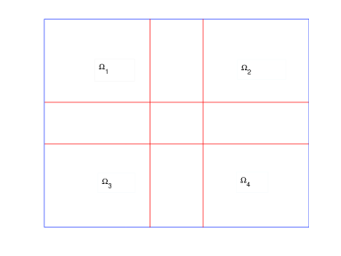
Figure 2.1: Domain $\Omega$ with its $4$ overlapping subdomains $\Omega_{1},\Omega_{2},\Omega_{3},\Omega_{4}$

Based on the partition of $\Omega$ into $4$ overlapping subdomains, we shall often need a local subspace of $L^{2}(\Omega)$ on each subdomain $\Omega_{i}$:

$$V_{i}=\Big{\{}f\in L^{2}(\Omega);~{}{\rm supp}(f)\subset\Omega_{i}\Big{\}},\,\quad\,i=1,\,2,\,3,\,4.$$

Next we start to derive some new DD algorithms for solving the optimization system (2.6). The algorithms are based on the local optimizations on the subspaces $V_{i}$ associated with subdomain $\Omega_{i}$. For some given $f_{j}\in V_{j}$ ($j=1,2,3,4$), let us consider the following local minimization over $\Omega_{i}$:

$$\min_{v_{i}\in V_{i}}J\Big{(}v_{i}+\sum_{j\neq i}f_{j}\Big{)}\,.$$ (2.7)

Here and in the sequel, we often write $\sum_{j=1,j\neq i}^{4}$ as $\sum_{j\neq i}$ for simplicity. By the definition of $J$ in (2.6) we know that each local update $v_{i}$ in $\Omega_{i}$ still needs to compute the quantity $U(v_{i}+\sum_{j\neq i}f_{j})$, which involves the solution of the forward system (2.3) in the entire domain $\Omega$. To avoid this, we construct an auxiliary functional $\tilde{J}_{i}^{s}$ of $J$, called the surrogate functional in [6], by introducing an auxiliary variable $a$. For a given $a\in V_{i}$ and $f_{j}\in V_{j}$ ($j=1,2,3,4$), we define

$$\tilde{J}_{i}^{s}(\sum_{j=1}^{4}f_{j},a)=J(\sum_{j=1}^{4}f_{j})+A\,\|f_{i}-a\|_{\Omega}^{2}-\|U(f_{i}-a)\|_{\Omega}^{2}$$ (2.8)

where $A$ is a positive constant to be selected such that

$$A\|f_{i}-a\|_{\Omega}^{2}-\|U(f_{i}-a)\|_{\Omega}^{2}\geq(A-\|U\|^{2})\|f_{i}-a\|_{\Omega}^{2}\geq 0\,.$$ (2.9)

This implies for any $f=\sum_{j=1}^{4}f_{j}$ that $\tilde{J}_{i}^{s}(f,a)=J(f)$ when $a=f_{i}$, and

$$J(f)=\tilde{J}_{i}^{s}(f,f_{i})\leq\tilde{J}_{i}^{s}(f,a)=J(f)+A\|f_{i}-a\|_{\Omega}^{2}-\|U(f_{i}-a)\|_{\Omega}^{2}\quad\forall\,a\in V_{i}\,.$$ (2.10)

So $\tilde{J}_{i}^{s}(f,a)$ can be viewed as a small perturbation of $J(f)$ when $a$ is close to $f_{i}$.

Now we shall convert (2.8) into a more explicit representation. Using (2.6), (2.8) and the adjoint relation (2.5) we can rewrite $\tilde{J}_{i}^{s}$ as follows:

$$\tilde{J}_{i}^{s}(\sum_{j=1}^{4}f_{j},a) = \|U(f_{i})\|_{\Omega}^{2}-2\langle f_{i},\,U(z_{0}^{\delta}-U(\sum_{j\neq i}f_{j})\rangle_{\Omega}+\|z_{0}^{\delta}-U(\sum_{j\neq i}f_{j})\|^{2}_{\Omega}+\beta\|\sum_{j=1}^{4}f_{j}\|_{\Omega}^{2}$$ (2.11)

$$+A\langle f_{i},\,f_{i}-2a\rangle_{\Omega}+A\|a\|_{\Omega}^{2}-\|U(f_{i})\|_{\Omega}^{2}+2\langle f_{i},\,U(U(a))\rangle_{\Omega}-\|U(a)\|_{\Omega}^{2}$$

$$= A\Big{\langle}f_{i},\,f_{i}-2\Big{\{}a+\frac{1}{A}U\Big{(}z_{0}^{\delta}-U(\sum_{j\neq i}f_{j})-U(a)\Big{)}\Big{\}}\Big{\rangle}_{\Omega_{i}}$$

$$+\beta\|\sum_{j=1}^{4}f_{j}\|_{\Omega}^{2}+\|z_{0}^{\delta}-U(\sum_{j\neq i}f_{j})\|^{2}_{\Omega}+A\|a\|_{\Omega}^{2}-\|U(a)\|_{\Omega}^{2}$$

$$= A\|f_{i}-\Big{\{}a+\frac{1}{A}U\Big{(}z_{0}^{\delta}-U(\sum_{j\neq i}f_{j}+a)\Big{)}\Big{\}}\|_{\Omega_{i}}^{2}+\beta\|\sum_{j=1}^{4}f_{j}\|_{\Omega}^{2}$$

$$+\Big{\{}\|z_{0}^{\delta}-U(\sum_{j\neq i}f_{j})\|^{2}_{\Omega}+A\|a\|_{\Omega}^{2}-\|U(a)\|_{\Omega}^{2}$$

$$-A\|a+\frac{1}{A}U\Big{(}z_{0}^{\delta}-U(\sum_{j\neq i}f_{j}+a)\Big{)}\|_{\Omega_{i}}^{2}\Big{\}}\,.$$

We can see that the last two terms in (2.11) does not depend on $f_{i}$, so it will not affect the local minimization over $\Omega_{i}$ if we drop them in the functional $\tilde{J}_{i}^{s}$. This leads us to consider the following functional for a given $a\in V_{i}$:

$$\min_{f_{i}\in V_{i}}\tilde{J}_{i}^{s}(f_{i}+\sum_{j\neq i}f_{j},a)=\min_{f_{i}\in V_{i}}A\|f_{i}-\tilde{z}_{i}\|_{\Omega_{i}}^{2}+\beta\|\sum_{j=1}^{4}f_{j}\|_{\Omega}^{2}$$ (2.12)

where $\tilde{z}_{i}$ is given by

$$\tilde{z}_{i}=a+\frac{1}{A}U(z_{0}^{\delta}-U(\sum_{j\neq i}f_{j}+a)).$$ (2.13)

Noting that (2.12) is a simple quadratic minimization, we can find its exact minimizer $f_{i}^{*}$:

$$f_{i}^{*}=\frac{1}{A+\beta}\Big{(}A\tilde{z}_{i}-\beta\sum_{j\neq i}f_{j}\Big{)}|_{\Omega_{i}}.$$ (2.14)

Clearly, the new functional $\tilde{J}_{i}^{s}$ in (2.12) has an obvious advantage over the functional $J$ in (2.6) or (2.7): it is completely local, and the minimization can be solved explicitly within the subdomain $\Omega_{i}$. However, for the solution of the local minimization (2.12) we need the data $\tilde{z}_{i}$ from (2.13), which involves the evaluations of $U(\sum_{j\neq i}f_{j}+a)$ and $U(z_{0}^{\delta}-U(\sum_{j\neq i}f_{j}+a))$. Unfortunately, these two evaluations are both global, and require the solutions of the forward system (2.3) in the entire domain $\Omega$. This is surely not expected in an efficient DD algorithm.

Next, we shall propose some techniques to get rid of the aforementioned two global evaluations so that the resulting DD algorithm involves only local minimizations over the local subdomains. For convenience, we write the boundary of $\Omega_{i}$ inside $\Omega$ by $\tilde{\Gamma}_{i}$, i.e., $\tilde{\Gamma}_{i}=\partial\Omega_{i}\cap\Omega$ for $i=1,2,3,4$. Then we introduce a local forward operator $U_{i}(f,p)$ associated with the forward problem (2.3):

$$\left\{\begin{array}[]{clclc}-\nabla\cdot(a({\bf x})\nabla U_{i}(f,\,p))+c({\bf x})U_{i}(f,\,p)&=&f&\mbox{in}&\Omega_{i},\\ U_{i}(f,p)&=&0&\mbox{on}&\partial\Omega\cap\partial\Omega_{i}\\ U_{i}(f,p)&=&p&\mbox{on}&\tilde{\Gamma}_{i}.\end{array}\right.$$ (2.18)

Clearly we can split $U_{i}(f,p)$ as $U_{i}(f,p)=U_{i}(f,0)+U_{i}(0,p)$, and $U_{i}(f,0)$ is self-adjoint, i.e.,

$$\langle U_{i}(f,0),\,\omega\rangle_{\Omega_{i}} = \langle f,\,U_{i}(\omega,0)\rangle_{\Omega_{i}}\quad\forall\,\omega\in L^{2}(\Omega_{i}).$$ (2.19)

Using the local operators $U_{i}(f,p)$ in (2.18), we introduce the following local functional for $f_{j}\in V_{j}$, $j=1,2,3,4$:

$$J_{i}(\sum_{j=1}^{4}f_{j},p) = \|U_{i}(\sum_{j=1}^{4}f_{j},p)-z_{0}^{\delta}\|_{\Omega_{i}}^{2}+\beta\|\sum_{j=1}^{4}f_{j}\|_{\Omega_{i}}^{2}\,,$$

and its surrogate functional $J_{i}^{s}$ for any given $a\in V_{i}$:

$$J_{i}^{s}(\sum_{j=1}^{4}f_{j},p,a)=J_{i}(\sum_{j=1}^{4}f_{j},p)+A\|f_{i}-a\|_{\Omega_{i}}^{2}-\|U_{i}(f_{i}-a,0)\|_{\Omega_{i}}^{2}\,.$$

Using the important fact that $U_{i}(\sum_{j=1}^{4}f_{j},p)=U_{i}(\sum_{j\neq i}f_{j},p)+U_{i}(f_{i},0)$ and the adjoint relation (2.19), we can write

$$J_{i}^{s}(\sum_{j=1}^{4}f_{j},p,a) = \|U_{i}(f_{i},0)\|_{\Omega_{i}}^{2}-2\langle f_{i},\,U_{i}\Big{(}z_{0}^{\delta}-U_{i}(\sum_{j\neq i}f_{j},p),0\Big{)}\rangle_{\Omega_{i}}$$ (2.20)

$$+\|z_{0}^{\delta}-U_{i}(\sum_{j\neq i}f_{j},p)\|^{2}_{\Omega_{i}}+\beta\|\sum_{j=1}^{4}f_{j}\|_{\Omega_{i}}^{2}+A\langle f_{i},\,f_{i}-2a\rangle_{\Omega_{i}}+A\|a\|_{\Omega_{i}}^{2}$$

$$-\|U_{i}(f_{i},0)\|_{\Omega_{i}}^{2}+2\langle f_{i},\,U_{i}(U_{i}(a,0),0)\rangle_{\Omega_{i}}-\|U_{i}(a,0)\|_{\Omega_{i}}^{2}$$

$$= A\langle f_{i},\,f_{i}-2\Big{\{}a+\frac{1}{A}U_{i}\Big{(}z_{0}^{\delta}-U_{i}(\sum_{j\neq i}f_{j}+a,p),0\Big{)}\Big{\}}\rangle_{\Omega_{i}}+\beta\|\sum_{j=1}^{4}f_{j}\|_{\Omega_{i}}^{2}$$

$$+\|z_{0}^{\delta}-U_{i}(\sum_{j\neq i}f_{j},p)\|^{2}_{\Omega_{i}}+A\|a\|_{\Omega_{i}}^{2}-\|U_{i}(a,0)\|_{\Omega_{i}}^{2}$$

$$= A\|f_{i}-\Big{\{}a+\frac{1}{A}U_{i}\Big{(}z_{0}^{\delta}-U_{i}(\sum_{j\neq i}f_{j}+a,p),0\Big{)}\Big{\}}\|_{\Omega_{i}}^{2}+\beta\|\sum_{j=1}^{4}f_{j}\|_{\Omega_{i}}^{2}$$

$$+\Big{\{}\|z_{0}^{\delta}-U_{i}(\sum_{j\neq i}f_{j},p)\|^{2}_{\Omega_{i}}+A\|a\|_{\Omega_{i}}^{2}-\|U_{i}(a,0)\|_{\Omega_{i}}^{2}$$

$$-A\|a+\frac{1}{A}U_{i}\Big{(}z_{0}^{\delta}-U_{i}(\sum_{j\neq i}f_{j}+a,p),0\Big{)}\|_{\Omega_{i}}^{2}\Big{\}},$$

We can easily see that the last term above does not depend on $f_{i}$, so it will not affect the local minimization over $\Omega_{i}$ if we drop them in the functional $J_{i}^{s}$. This leads us to consider the following functional for a given $a\in V_{i}$:

$$\min_{f_{i}\in V_{i}}J_{i}^{s}(\sum_{j=1}^{4}f_{j},p,a)=\min_{f_{i}\in V_{i}}A\|f_{i}-z_{i}\|_{\Omega_{i}}^{2}+\beta\|\sum_{j=1}^{4}f_{j}\|_{\Omega_{i}}^{2},$$ (2.21)

where $z_{i}=a+\frac{1}{A}U_{i}\Big{(}z_{0}^{\delta}-U_{i}(\sum_{j\neq i}f_{j}+a,p),0\Big{)}$. (2.21) is a simple quadratic minimization, and we can find its exact minimizer $f_{i}^{*}$:

$$f_{i}^{*}=\frac{1}{A+\beta}\Big{\{}A\,a+U_{i}\Big{(}z_{0}^{\delta}-U_{i}(\sum_{j\neq i}f_{j}+a,p),0\Big{)}-\beta\sum_{j\neq i}f_{j}|_{\Omega_{i}}\Big{\}}.$$ (2.22)

We can see from this expression that as long as the inner boundary value $p$ is available, the minimization (2.21) does not involve any global data and is completely local. Noting that $U(f)|_{\Omega_{i}}=U_{i}(f,U(f))$ and the definitions of $J_{i}(f,p)$ and $J_{i}^{s}(f,p,a)$, we can connect $J_{i}(f,p)$ and $J_{i}^{s}(f,p,a)$ with functional $J(f)$ (cf. (2.6)) restricted in $\Omega_{i}$:

$$\|U(\sum_{j=1}^{4}f_{j})-z^{\delta}_{0}\|_{\Omega_{i}}^{2}+\beta\|\sum_{j=1}^{4}f_{j}\|_{\Omega_{i}}^{2}$$ (2.23)

$$= \|U_{i}(\sum_{j=1}^{4}f_{j},U(\sum_{j=1}^{4}f_{j}))-z^{\delta}_{0}\|_{\Omega_{i}}^{2}+\beta\|\sum_{j=1}^{4}f_{j}\|_{\Omega_{i}}^{2}$$

$$= J_{i}(\sum_{j=1}^{4}f_{j},U(\sum_{j=1}^{4}f_{j}))=J_{i}^{s}(\sum_{j=1}^{4}f_{j},U(\sum_{j=1}^{4}f_{j}),f_{i}).$$

So using (2.21), we are now ready to apply the multiplicative or additive Schwarz iteration principle [11] [14] to establish two DD algorithms for solving the optimization system (2.6). For the description of the algorithms, we introduce an index function for any point ${\bf x}\in\Omega$:

$$n({\bf x})=\Big{\{}i;\,{\bf x}\in\Omega_{i},~{}i\in\{1,2,3,4\}\Big{\}}\,;\quad|n({\bf x})|=~{}\mbox{number of elements in}~{}n({\bf x})\,.$$ (2.24)

Algorithm 2.1 (Multiplicative Schwarz Algorithm (MSA))

Choose a tolerance parameter $\epsilon_{1}>0$, an initial value $f^{(0)}=\sum_{i=1}^{4}f_{i}^{(0)}$ with $f_{i}^{(0)}\in V_{i}$ ($i=1,2,3,4$), and solve (2.3) for $U(f^{(0)})$; set $p_{i}^{(0)}:=U(f^{(0)})|_{\tilde{\Gamma}_{i}}$ and $n:=0$.

1. Compute $f_{i}^{(n+1)}\in V_{i}$ sequentially for $i=1$ to $4$ by

   $$f_{i}^{(n+1)}={\rm argmin}_{v_{i}\in V_{i}}J_{i}^{s}(\sum_{j<i}f_{j}^{(n+1)}+v_{i}+\sum_{j>i}f_{j}^{(n)},p_{i}^{(n)},f_{i}^{(n)});$$ (2.25)

   update $U_{i}$ in $\Omega_{i}$:

   $$U_{i}^{(n)}=U_{i}(\sum_{j\leq i}f_{j}^{(n+1)}+\sum_{j>i}f_{j}^{(n)},p_{i}^{(n)});$$

   update the inner boundary values on $\tilde{\Gamma}_{j}$ for $j>i$ if $\tilde{\Gamma}_{j}\in\Omega_{i}$:

   $$p_{j}^{(n)}=U_{i}^{(n)}|_{\tilde{\Gamma}_{j}}\,.$$

2. Compute $f^{(n+1)}=\sum_{i=1}^{4}f_{i}^{(n+1)}$.

3. If $\|f^{(n+1)}-f^{(n)}\|_{\Omega}\leq\epsilon_{1}$, stop the iteration;

   otherwise update $U_{i}$ in subdomain $\Omega_{i}$ ($i=1,2,3,4$):

   $$U_{i}^{(n+1)}=U_{i}(f^{(n+1)},p_{i}^{(n)});$$

   update the inner boundary values on $\tilde{\Gamma}_{i}$ ($i=1,2,3,4$):

   $$p_{i}^{(n+1)}({\bf x})=\frac{1}{|n({\bf x})|}\sum_{j\in n({\bf x})}U_{j}^{(n+1)}({\bf x}),\,\ \forall\,{\bf x}\in\tilde{\Gamma}_{i}.$$

   set $n:=n+1$, go to Step 1.

We can easily see that Algorithm 2.1 is sequential or multiplicative. The next algorithm proposes a parallel version of Algorithm 2.1. For this purpose, we introduce a bounded uniform partition of unity $\{\chi_{i}\}_{i=1}^{4}$ such that $\sum_{i=1}^{4}\chi_{i}=1$ and $\|\chi_{i}\|_{\infty}\leq 1$ and ${\rm supp}(\chi_{i})\subset\Omega_{i}$.

Algorithm 2.2 (Additive Schwarz Algorithm (ASA))

Choose a tolerance parameter $\epsilon_{1}>0$, a relaxation parameter $\lambda\in(0,1)$, an initial value $f^{(0)}=\sum_{i=1}^{4}f_{i}^{(0)}$ with $f_{i}^{(0)}\in V_{i}$ ($i=1,2,3,4$), and solve (2.3) for $U(f^{(0)})$; set $p_{i}^{(0)}:=U(f^{(0)})|_{\tilde{\Gamma}_{i}}$ and $n:=0$.

1. Compute $f_{i}^{(n+1)}\in V_{i}$ in parallel for $i=1,2,3,4$ by

   $$f_{i}^{(n+1)}={\rm argmin}_{v_{i}\in V_{i}}J_{i}^{s}(\sum_{j\neq i}f_{j}^{(n)}+v_{i},p_{i}^{(n)},f_{i}^{(n)}).$$ (2.26)

2. Compute $f^{(n+1)}=\lambda\sum_{i=1}^{4}f_{i}^{(n+1)}+(1-\lambda)f^{(n)}$.

3. If $\|f^{(n+1)}-f^{(n)}\|_{\Omega}\leq\epsilon_{1}$, stop the iteration;

   otherwise update $U_{i}$ in subdomains $\Omega_{i}$ ($i=1,2,3,4$):

   $$U_{i}^{(n+1)}=U_{i}(f^{(n+1)},p_{i}^{(n)});$$

   update the inner boundary values on $\tilde{\Gamma}_{i}$ ($i=1,2,3,4$):

   $$p_{i}^{(n+1)}({\bf x})=\frac{1}{|n({\bf x})|}\sum_{j\in n({\bf x})}U_{j}^{(n+1)}({\bf x})\quad\forall\,{\bf x}\in\tilde{\Gamma}_{i}.$$

   set $f_{i}^{(n+1)}:=\chi_{i}f^{(n+1)}$, and $n:=n+1$, go to Step 1.

Remark 2.1

The same as for (2.22) we have explicit expressions for the minimizers $f_{i}^{(n+1)}$ in (2.25) and (2.26). In our numerical implementations, we will simply take the partition of unity $\{\chi_{i}\}_{i=1}^{4}$ used in Algorithm 2.2 as follows:

$$\chi_{i}({\bf x})={1}/{|n({\bf x})|}\quad\mbox{for}\quad{\bf x}\in\Omega_{i}\,;\quad\chi_{i}({\bf x})=0\quad\mbox{for}\quad{\bf x}\in\Omega\backslash\bar{\Omega}_{i}.$$

3 Domain decomposition algorithms for flux reconstruction

In this section, we propose a DD algorithm to solve the inverse problem of identifying fluxes on part of the boundary. Let $\Omega\subset R^{d}~{}(d\geq 1)$ be an open bounded and connected domain, with a boundary $\partial\Omega$, which splits into two parts, i.e., $\partial\Omega=\Gamma_{0}\cup\Gamma_{1}$. Then we consider the following elliptic system

$$\left\{\begin{array}[]{rclll}-\nabla\cdot(a({\bf x})\nabla u)+c({\bf x})u&=&f({\bf x})&\mbox{in}&\Omega\,,\\ a({\bf x})\frac{\partial u}{\partial n}&=&g({\bf x})&\mbox{on}&\Gamma_{0}\,,\\ a({\bf x})\frac{\partial u}{\partial n}&=&h({\bf x})&\mbox{on}&\Gamma_{1}\,,\end{array}\right.$$ (3.1)

where $a({\bf x})$, $c({\bf x})$, $f({\bf x})$, $g({\bf x})$ are all given functions, and $a({\bf x})\geq a_{1}>0$, $c({\bf x})\geq c_{1}>0$ in $\Omega$. Suppose that the flux $h({\bf x})$ of the model system is unknown on the inaccessible part $\Gamma_{1}$ of $\partial\Omega$, our inverse problem is to recover the flux distribution on $\Gamma_{1}$ when some measurement data $u^{\delta}$ of $u$ is available on the accessible part $\Gamma_{0}$ of $\partial\Omega$. We shall write the solution of system (3.1) as $u(h)$ to emphasize its dependence on the flux $h({\bf x})$.

As discussed in section 2, we formulate the ill-posed inverse problem of recovering the flux into a mathematically stabilized minimization system of the form

$$\min_{h\in L^{2}(\Gamma_{1})}J(h) = \|u(h)-z^{\delta}\|_{\Gamma_{0}}^{2}+\beta\|h\|_{\Gamma_{1}}^{2}\,.$$ (3.2)

This formulation is stable in the sense that the minimizer $h$ to (3.2) depends continuously on the change of the noise in the data $u^{\delta}$ [12].

Similarly to the discussions in Section 2, we can write the solution $u(h)$ to (3.1) as

$$u(h)=U(h)+u(0)\,,$$ (3.3)

where $U(h)$ is the solution to the following system:

$$\left\{\begin{array}[]{rclll}-\nabla\cdot(a({\bf x})\nabla U)+c({\bf x})U&=&0&\mbox{in}&\Omega,\\ a({\bf x})\frac{\partial U}{\partial n}&=&0&\mbox{on}&\Gamma_{0},\\ a({\bf x})\frac{\partial U}{\partial n}&=&h&\mbox{on}&\Gamma_{1}\,.\end{array}\right.$$ (3.4)

Adjoint operator of $U(h)$. For any $\omega\in L^{2}(\Gamma_{0})$, consider the solution $U^{*}(\omega)\in H^{1}(\Omega)$ to the following system:

$$\left\{\begin{array}[]{rclll}-\nabla\cdot(a({\bf x})\nabla U^{*}(\omega))+c({\bf x})U^{*}(\omega)&=&0&\mbox{in}&\Omega,\\ a({\bf x})\frac{\partial U^{*}(\omega)}{\partial n}&=&\omega&\mbox{on}&\Gamma_{0},\\ a({\bf x})\frac{\partial U^{*}(\omega)}{\partial n}&=&0&\mbox{on}&\Gamma_{1}.\end{array}\right.$$ (3.5)

This mapping $U^{*}:L^{2}(\Gamma_{0})\rightarrow L^{2}(\Gamma_{1})$ is the adjoint operator of $U$, namely, it holds that

$$\langle U(h),\,\omega\rangle_{\Gamma_{0}}=\langle h,\,U^{*}(\omega)\rangle_{\Gamma_{1}}\,\quad\forall\,\omega\in L^{2}(\Gamma_{0}).$$ (3.6)

This relation follows directly from (3.4), (3.5) and an application of integration by parts:

$$\langle U(h),\,\omega\rangle_{\Gamma_{0}}=\langle U(h),a({\bf x})\frac{\partial U^{*}(\omega)}{\partial n}\rangle_{\Gamma_{0}}$$

$$= \langle U(h),\,a({\bf x})\frac{\partial U^{*}(\omega)}{\partial n}\rangle_{\partial\Omega}+\int_{\Omega}U(h)(-\nabla\cdot(a({\bf x})\nabla U^{*}(\omega))+c({\bf x})U^{*}(\omega))d{\bf x}$$

$$= \int_{\Omega}(-\nabla\cdot(a({\bf x})\nabla U(h))+c({\bf x})U(h))U^{*}(\omega)d{\bf x}+\langle a({\bf x})\frac{\partial U(h)}{\partial n},\,U^{*}(\omega)\rangle_{\partial\Omega}$$

$$= \langle a({\bf x})\frac{\partial U(h)}{\partial n},\,U^{*}(\omega)\rangle_{\Gamma_{1}}=\langle h,\,U^{*}(\omega)\rangle_{\Gamma_{1}}.$$

3.1 DD algorithms with explicit local solvers

In this subsection, we follow section 2.1 to derive some overlapping domain decomposition method for solving the minimization in (3.2). As in section 2.1, $\Omega$ is divided into the overlapping subdomains $\Omega_{i}$ ($i=1,2,3,4$), accordingly the feasible constraint space $L^{2}(\Gamma_{1})$ can be decomposed into the subspaces

$$V_{i}=\Big{\{}h\in L^{2}(\Gamma_{1});~{}{\rm supp}(h)\subset\partial\Omega_{i}\cap\Gamma_{1}\Big{\}},\,\quad\,i=1,\,2,\,3,\,4.$$

Next we introduce an auxiliary surrogate functional $\tilde{J}_{i}^{s}$ of $J(h)$ in (3.2) for any given $a\in V_{i}$ and $h_{j}\in V_{j}$ ($j=1,2,3,4$):

$$\tilde{J}_{i}^{s}(\sum_{j=1}^{4}h_{j},a)=J(\sum_{j=1}^{4}h_{j})+A\|h_{i}-a\|_{\Gamma_{1}}^{2}-\|U(h_{i}-a)\|_{\Gamma_{0}}^{2}.$$ (3.7)

By similar derivations to (2.11) but using the adjoint relation (3.6), we can rewrite $\tilde{J}_{i}^{s}$ as

$$\tilde{J}_{i}^{s}(\sum_{j=1}^{4}h_{j},a) = A\|h_{i}-\Big{\{}a+\frac{1}{A}U^{*}\Big{(}z_{0}^{\delta}-U(\sum_{j\neq i}h_{j}+a)\Big{)}\Big{\}}\|_{\partial\Omega_{i}\cap\Gamma_{1}}^{2}+\beta\|\sum_{j=1}^{4}h_{j}\|_{\Gamma_{1}}^{2}$$ (3.8)

$$+\Big{\{}\|z_{0}^{\delta}-U(\sum_{j\neq i}h_{j})\|^{2}_{\Gamma_{0}}+A\|a\|_{\Gamma_{1}}^{2}-\|U(a)\|_{\Gamma_{0}}^{2}$$

$$-A\|a+\frac{1}{A}U^{*}\Big{(}z_{0}^{\delta}-U(\sum_{j\neq i}h_{j}+a)\Big{)}\|_{\partial\Omega_{i}\cap\Gamma_{1}}^{2}\Big{\}},$$

where $z_{0}^{\delta}=z^{\delta}-u(0)$. We can see that the last two terms do not depend on $h_{i}$, so we can drop them in the minimization of functional $\tilde{J}_{i}^{s}$. Hence it leads us to the following local minimization for any $a\in V_{i}$:

$$\min_{h_{i}\in V_{i}}\tilde{J}_{i}^{s}(h_{i}+\sum_{j\neq i}h_{j},a)=\min_{h_{i}\in V_{i}}A\|h_{i}-\tilde{z}_{i}\|_{\partial\Omega_{i}\cap\Gamma_{1}}^{2}+\beta\|\sum_{j=1}^{4}h_{j}\|_{\Gamma_{1}}^{2}$$ (3.9)

where $\tilde{z}_{i}$ is given by

$$\tilde{z}_{i}=a+\frac{1}{A}U^{*}(z_{0}^{\delta}-U(\sum_{j\neq i}h_{j}+a)).$$ (3.10)

This is a quadratic minimization, so we can find its exact minimizer $h_{i}^{*}$:

$$h_{i}^{*}=\frac{1}{A+\beta}\Big{(}A\tilde{z}_{i}-\beta\sum_{j\neq i}h_{j}\Big{)}\Big{|}_{\partial\Omega_{i}\cap\Gamma_{1}}.$$ (3.11)

We observe that the minimization (3.9) is completely local, and its solution can be achieved explicitly within the subdomain $\Omega_{i}$. However, its solution $h_{i}^{*}$ needs the data $\tilde{z}_{i}$ from (3.10), which involves two global solutions of the forward and adjoint systems (3.4) and (3.5), and is clearly not expected in an efficient DD algorithm. Next, we propose some techniques to avoid these two global evaluations so that the resulting DD algorithm involves only local minimizations over the local subdomains. To do so, we introduce two local forward and adjoint operators $U_{i}(h,p)$ and $U^{*}_{i}(\omega,q)$ associated with the global forward and adjoint systems (3.4) and (3.5):

$$\left\{\begin{array}[]{clclc}-\nabla\cdot(a({\bf x})\nabla U_{i}(h,p))+c({\bf x})U_{i}(h,p)&=&0&\mbox{in}&\Omega_{i},\\ a({\bf x})\frac{\partial U_{i}(h,p)}{\partial n}&=&0&\mbox{on}&\Gamma_{0}\cap\partial\Omega_{i},\\ a({\bf x})\frac{\partial U_{i}(h,p)}{\partial n}&=&h&\mbox{on}&\Gamma_{1}\cap\partial\Omega_{i},\\ U_{i}(h,p)&=&p&\mbox{on}&\tilde{\Gamma}_{i}\end{array}\right.$$ (3.12)

and

$$\left\{\begin{array}[]{clclc}-\nabla\cdot(a({\bf x})\nabla U^{*}_{i}(\omega,q))+c({\bf x})U^{*}_{i}(\omega,q)&=&0&\mbox{in}&\Omega_{i},\\ a({\bf x})\frac{\partial U^{*}_{i}(\omega,q)}{\partial n}&=&\omega&\mbox{on}&\Gamma_{0}\cap\partial\Omega_{i},\\ a({\bf x})\frac{\partial U^{*}_{i}(\omega,q)}{\partial n}&=&0&\mbox{on}&\Gamma_{1}\cap\partial\Omega_{i},\\ U^{*}_{i}(\omega,q)&=&q&\mbox{on}&\tilde{\Gamma}_{i}.\end{array}\right.$$ (3.13)

Using the systems (3.12), (3.13) and the integration by parts formula, we derive the following important relation that will be needed later on:

$$\langle U_{i}(h,0),\,\omega\rangle_{\Gamma_{0}\cap\partial\Omega_{i}} = \langle h,\,U^{*}_{i}(\omega,0)\rangle_{\Gamma_{1}\cap\partial\Omega_{i}}\quad\forall\,\omega\in L^{2}(\Gamma_{0}\cap\partial\Omega_{i}).$$ (3.14)

By means of the local operators $U_{i}(h,p)$ in (3.12), we introduce the local functional $J_{i}(\sum_{j=1}^{4}h_{j},p)$ for $h_{j}\in V_{j}$ ($j=1,2,3,4$):

$$J_{i}(\sum_{j=1}^{4}h_{j},p) = \|U_{i}(\sum_{j=1}^{4}h_{j},p)-z_{0}^{\delta}\|_{\Gamma_{0}\cap\partial\Omega_{i}}^{2}+\beta\|\sum_{j=1}^{4}h_{j}\|_{\Gamma_{1}\cap\partial\Omega_{i}}^{2}\,,$$

and a surrogate functional $J_{i}^{s}$ for a given $a\in V_{i}$:

$$J_{i}^{s}(\sum_{j=1}^{4}h_{j},p,a) = J_{i}(\sum_{j=1}^{4}h_{j},p)+A\|h_{i}-a\|_{\Gamma_{1}\cap\partial\Omega_{i}}^{2}-\|U_{i}(h_{i}-a,0)\|_{\Gamma_{0}\cap\partial\Omega_{i}}^{2}\,.$$ (3.15)

Using the important fact that $U_{i}(\sum_{j=1}^{4}h_{j},p)=U_{i}(\sum_{j\neq i}h_{j},p)+U_{i}(h_{i},0)$ and the adjoint relation (3.14), we can rewrite $J_{i}^{s}(\sum_{j=1}^{4}h_{j},p,a)$ as

$$J_{i}^{s}(\sum_{j=1}^{4}h_{j},p,a) = A\|h_{i}-\Big{\{}a+\frac{1}{A}U^{*}_{i}\Big{(}z_{0}^{\delta}-U_{i}(\sum_{j\neq i}h_{j}+a,p),0\Big{)}\Big{\}}\|_{\Gamma_{1}\cap\partial\Omega_{i}}^{2}+\beta\|\sum_{j=1}^{4}h_{j}\|_{\Gamma_{1}\cap\partial\Omega_{i}}^{2}$$ (3.16)

$$+\Big{\{}\|z_{0}^{\delta}-U_{i}(\sum_{j\neq i}h_{j},p)\|^{2}_{\Gamma_{0}\cap\partial\Omega_{i}}+A\|a\|_{\Gamma_{1}\cap\partial\Omega_{i}}^{2}-\|U_{i}(a,0)\|_{\Gamma_{0}\cap\partial\Omega_{i}}^{2}$$

$$-A\|a+\frac{1}{A}U^{*}_{i}\Big{(}z_{0}^{\delta}-U_{i}(\sum_{j\neq i}h_{j}+a,p),0\Big{)}\|_{\Gamma_{1}\cap\partial\Omega_{i}}^{2}\Big{\}}\,.$$

As the last term does not depend on $h_{i}$, we are led to the following quadratic minimization:

$$\min_{h_{i}\in V_{i}}J_{i}^{s}(\sum_{j=1}^{4}h_{j},p,a)=\min_{h_{i}\in V_{i}}A\|h_{i}-z_{i}\|_{\Gamma_{1}\cap\partial\Omega_{i}}^{2}+\beta\|\sum_{j=1}^{4}h_{j}\|_{\Gamma_{1}\cap\partial\Omega_{i}}^{2}$$ (3.17)

where $z_{i}$ is given by

$$z_{i}=a+\frac{1}{A}U^{*}_{i}\Big{(}z_{0}^{\delta}-U_{i}(\sum_{j\neq i}h_{j}+a,p),0\Big{)}.$$

We can easily find the minimizer to the quadratic optimization (3.17) in an explicit form:

$$h_{i}^{*}=\frac{1}{A+\beta}\Big{\{}Aa+U^{*}_{i}\Big{(}z_{0}^{\delta}-U_{i}(\sum_{j\neq i}h_{j}+a,p),0\Big{)}-\beta\sum_{j\neq i}h_{j}|_{\Gamma_{1}\cap\partial\Omega_{i}}\Big{\}}.$$ (3.18)

As in Section 2.1, we are now ready to formulate two new DD algorithms for the minimization system (3.2) for identifying the heat flux. For the description of the DD algorithms, we introduce an index function for any point ${\bf x}\in\Gamma_{1}$:

$$n({\bf x})=\Big{\{}i;\,{\bf x}\in\partial\Omega_{i}\cap\Gamma_{1},~{}i\in\{1,2,3,4\}\Big{\}}\,;\quad|n({\bf x})|=~{}\mbox{number of elements in}~{}n({\bf x})\,.$$

Algorithm 3.1 (Multiplicative Schwarz Algorithm (MSA))

Choose a tolerance parameter $\epsilon_{1}>0$, an initial value $h^{(0)}=\sum_{i=1}^{4}h_{i}^{(0)}$ with $h_{i}^{(0)}\in V_{i}$ ($i=1,2,3,4$), and solve (3.4) for $U(h^{(0)})$; set $p_{i}^{(0)}:=U(h^{(0)})|_{\tilde{\Gamma}_{i}}$ and $n:=0$.

1. Compute $h_{i}^{(n+1)}\in V_{i}$ sequentially for $i=1$ to $4$ by

   $$h_{i}^{(n+1)}={\rm argmin}_{v_{i}\in V_{i}}J_{i}^{s}(\sum_{j<i}h_{j}^{(n+1)}+v_{i}+\sum_{j>i}h_{j}^{(n)},p_{i}^{(n)},h_{i}^{(n)});$$ (3.19)

   update $U_{i}$ in $\Omega_{i}$:

   $$U_{i}^{(n)}=U_{i}(\sum_{j\leq i}h_{j}^{(n+1)}+\sum_{j>i}h_{j}^{(n)},p_{i}^{(n)});$$

   update the inner boundary values on $\tilde{\Gamma}_{j}$ for $j>i$ if $\tilde{\Gamma}_{j}\in\Omega_{i}$:

   $$p_{j}^{(n)}=U_{i}^{(n)}|_{\tilde{\Gamma}_{j}}\,.$$

2. Compute $h^{(n+1)}=\sum_{i=1}^{4}h_{i}^{(n+1)}$.

3. If $\|h^{(n+1)}-h^{(n)}\|_{\Gamma_{1}}\leq\epsilon_{1}$, stop the iteration;

   otherwise update $U_{i}$ in subdomains $\Omega_{i}$ ($i=1,2,3,4$):

   $$U_{i}^{(n+1)}=U_{i}(h^{(n+1)},p_{i}^{(n)});$$

   update the inner boundary values on $\tilde{\Gamma}_{i}$ ($i=1,2,3,4$):

   $$p_{i}^{(n+1)}({\bf x})=\frac{1}{|n({\bf x})|}\sum_{j\in n({\bf x})}U_{j}^{(n+1)}({\bf x}),\,\ \forall\,{\bf x}\in\tilde{\Gamma}_{i}.$$

   set $n:=n+1$, go to Step 1.

The next algorithm proposes a parallel version of Algorithm 3.1. For this purpose, we introduce a uniform partition of unity $\{\chi_{i}\}_{i=1}^{4}$ such that $\sum_{i=1}^{4}\chi_{i}=1$ and $\|\chi_{i}\|_{\infty}\leq 1$ and ${\rm supp}(\chi_{i})\subset\partial\Omega_{i}\cap\Gamma_{1}$.

Algorithm 3.2 (Additive Schwarz Algorithm (ASA))

Choose a tolerance parameter $\epsilon_{1}>0$, a relaxation parameter $\lambda\in(0,1)$, an initial value $h^{(0)}=\sum_{i=1}^{4}h_{i}^{(0)}$ with $h_{i}^{(0)}\in V_{i}$ ($i=1,2,3,4$), and solve (3.4) for $U(h^{(0)})$; set $p_{i}^{(0)}:=U(h^{(0)})|_{\tilde{\Gamma}_{i}}$ and $n:=0$.

1. Compute $h_{i}^{(n+1)}\in V_{i}$ in parallel for $i=1,2,3,4$ by

   $$h_{i}^{(n+1)}={\rm argmin}_{v_{i}\in V_{i}}J_{i}^{s}(\sum_{j\neq i}h_{j}^{(n)}+v_{i},p_{i}^{(n)},h_{i}^{(n)}).$$ (3.20)

2. Compute $h^{(n+1)}=\lambda\sum_{i=1}^{4}h_{i}^{(n+1)}+(1-\lambda)h^{(n)}$.

3. If $\|h^{(n+1)}-h^{(n)}\|_{\Gamma_{1}}\leq\epsilon_{1}$, stop the iteration;

   otherwise update $U_{i}$ in subdomains $\Omega_{i}$ ($i=1,2,3,4$):

   $$U_{i}^{(n+1)}=U_{i}(h^{(n+1)},p_{i}^{(n)});$$

   update the inner boundary values on $\tilde{\Gamma}_{i}$ ($i=1,2,3,4$):

   $$p_{i}^{(n+1)}({\bf x})=\frac{1}{|n({\bf x})|}\sum_{j\in n({\bf x})}U_{j}^{(n+1)}({\bf x})\quad\forall\,{\bf x}\in\tilde{\Gamma}_{i}.$$

   set $h_{i}^{(n+1)}:=\chi_{i}h^{(n+1)}$, and $n:=n+1$, go to Step 1.

Remark 3.1

The same as for (3.18), we have explicit expressions for the minimizers $h_{i}^{(n+1)}$ in (3.19) and (3.20). In our numerical implementations, we will simply take the partition of unity $\{\chi_{i}\}_{i=1}^{4}$ used in Algorithm 3.2 as follows: $\chi_{i}({\bf x})={1}/{|n({\bf x})|}$ for ${\bf x}\in\partial\Omega_{i}\cap\Gamma_{1}$, and $\chi_{i}({\bf x})=0$ for ${\bf x}\in\Gamma_{1}\backslash\partial\Omega_{i}$.

4 Domain decomposition algorithms for the reconstruction of an initial temperature

In this section, we are interested in extending the DD algorithms proposed in sections 2 and 3 for solving the stationary inverse source and flux problems to a time-dependent inverse problem, the identification of the initial temperature in the following heat conduction system:

$$\left\{\begin{array}[]{rcclc}u_{t}-\nabla\cdot(a({\bf x})\nabla u)&=&f({\bf x},t)&\mbox{in}&\,\,\Omega\times(0,\,T),\\ u&=&0{}{}&\mbox{on}&~{}\partial\Omega\times(0,\,T),\\ u({\bf x},0)&=&\varphi({\bf x})&{\rm in}&\,\,\Omega.\end{array}\right.$$ (4.1)

We assume that some observation data $z^{\delta}$ of the temperature $u({\bf x},t)$ are available in $\Omega$ or in some small subregion $\omega\subset\Omega$, but with a time history in the range $[T-\sigma,T]$. The inverse problem of our interest is to recover the initial temperature distribution $\varphi({\bf x})$, using the observation data $z^{\delta}$. We shall write the solution of system (4.1) as $u(\varphi)$ to emphasize its dependence on the initial temperature $\varphi({\bf x})$.

As described in Section 2, it is easy to verify that $u(\varphi)=U(\varphi)+u(0)$, where $U(\varphi)$ is linear with respect to $\varphi$ and satisfies the following system

$$\left\{\begin{array}[]{rclll}U_{t}-\nabla\cdot(a({\bf x})\nabla U)&=&0&\mbox{in}&\,\,\Omega\times(0,\,T),\\ U&=&0{}{}&\mbox{on}&~{}\partial\Omega\times(0,\,T),\\ U({\bf x},0)&=&\varphi({\bf x})&{\rm in}&\,\,\Omega,\end{array}\right.$$ (4.2)

whose variational formulation is given by

$$\int_{0}^{T}\int_{\Omega}U_{t}\psi d{\bf x}dt+\int_{0}^{T}\int_{\Omega}a({\bf x})\nabla U\cdot\nabla\psi d{\bf x}dt=0\quad\forall\,\,\psi\in L^{2}(0,T;H^{1}_{0}(\Omega))\,.$$ (4.3)

Let $z_{0}^{\delta}=z^{\delta}-u(0)$, then we can formulate our inverse problem as the following regularized output least-squares minimization:

$$\min_{\varphi\in L^{2}(\Omega)}J(\varphi)=\min_{\varphi\in L^{2}(\Omega)}\int_{T-\sigma}^{T}\|U(\varphi)-z_{0}^{\delta}\|_{L^{2}(\Omega)}^{2}dt+\beta\|\varphi\|_{L^{2}(\Omega)}^{2}.$$ (4.4)

Now we introduce the adjoint system of the forward problem (4.2):

$$\left\{\begin{array}[]{rcccc}U^{*}_{t}+\nabla\cdot(a({\bf x})\nabla U^{*})&=&0&\mbox{in}&\,\,\Omega\times(0,\,T),\\ U^{*}&=&0&\mbox{on}&~{}\partial\Omega\times(0,\,T),\\ U^{*}({\bf x},T)&=&\omega&{\rm in}&\,\,\Omega,\end{array}\right.$$ (4.5)

which is linear with respect to $\omega$. Next we derive a very useful relation:

$$\langle U(\varphi)({\bf x},t),\,\omega\rangle_{L^{2}(\Omega)}=\langle\varphi,\,U^{*}(\omega)({\bf x},T-t)\rangle_{L^{2}(\Omega)}\quad\forall\,t\in[0,T]\,.$$ (4.6)

Clearly, this is true for $t=0$ by the initial and terminal conditions in (4.2) and (4.5). To verify it for $t\in(0,T]$, we define $U^{*,s}(\omega)$ for $s\in(0,T]$:

$$\left\{\begin{array}[]{rcccc}U^{*,s}_{t}+\nabla\cdot(a({\bf x})\nabla U^{*,s})&=&0&\mbox{in}&\,\,\Omega\times(0,\,s),\\ U^{*,s}&=&0&\mbox{on}&~{}\partial\Omega\times(0,\,s),\\ U^{*,s}({\bf x},s)&=&\omega&{\rm in}&\,\,\Omega.\end{array}\right.$$ (4.7)

It is easy to find the following relation,

$$U^{*}(\omega)({\bf x},T-s)=U^{*,s}(\omega)({\bf x},0),$$ (4.8)

and the variational formulation of (4.7),

$$-\int_{0}^{s}\int_{\Omega}U^{*,s}_{t}\psi d{\bf x}dt+\int_{0}^{s}\int_{\Omega}a({\bf x})\nabla U^{*,s}\cdot\nabla\psi d{\bf x}dt=0\quad\forall\,\psi\in L^{2}(0,s;H^{1}_{0}(\Omega)).$$ (4.9)

Using $U^{*,s}$ in (4.7) and its property (4.8), we see (4.6) immediately from the following relation

$$\langle U(\varphi)({\bf x},s),\,\omega\rangle_{L^{2}(\Omega)}=\langle\varphi,\,U^{*,s}(\omega)({\bf x},0)\rangle_{L^{2}(\Omega)}\,.$$ (4.10)

To check this relation, we use (4.3) with the terminal time $T$ replaced by $s$, then take $\psi=U^{*,s}$ and integrate by parts with respect to $t$ to obtain

$$\int_{\Omega}U({\bf x},s)U^{*,s}({\bf x},s)d{\bf x}-\int_{\Omega}U({\bf x},0)U^{*,s}({\bf x},0)d{\bf x}-\int_{0}^{s}\int_{\Omega}UU^{*,s}_{t}d{\bf x}dt$$ (4.11)

$$+ \int_{0}^{s}\int_{\Omega}a({\bf x})\nabla U\cdot\nabla U^{*,s}d{\bf x}dt=0.$$

Now the desired relation (4.10) follows readily from the initial and terminal conditions in (4.2) and (4.7) and equation (4.9) with $\psi=U$.

Next we shall follow sections 2 and 3 to derive some overlapping domain decomposition method for solving the time-dependent minimization (4.4). As in section 2.1, $\Omega$ is divided into the overlapping subdomains $\Omega_{i}$ ($i=1,2,3,4$), accordingly the feasible constraint space $L^{2}(\Omega)$ can be decomposed into the following subspaces:

$$V_{i}=\Big{\{}\varphi\in L^{2}(\Omega);~{}~{}{\rm supp}(\varphi)\subset\Omega_{i}\Big{\}},\,\quad\,i=1,\,2,\,3,\,4.$$

In order to avoid any global solution of the forward and adjoint systems (4.2) and (4.5) in our DD algorithms, we introduce their local variants, namely, the solutions $U_{i}(\varphi,p)$ and $U_{i}^{*}(\omega,p)$ to the following systems:

$$\left\{\begin{array}[]{clclc}U_{i}(\varphi,p)({\bf x},t)_{t}-\nabla\cdot(a({\bf x})\nabla U_{i}(\varphi,p)({\bf x},t))&=&0&\mbox{in}&\Omega_{i}\times(0,\,T),\\ U_{i}(\varphi,p)({\bf x},t)&=&0&\mbox{on}&(\partial\Omega\cap\partial\Omega_{i})\times(0,\,T),\\ U_{i}(\varphi,p)({\bf x},t)&=&p({\bf x},t)&\mbox{on}&\tilde{\Gamma}_{i}\times(0,\,T),\\ U_{i}(\varphi,p)({\bf x},0)&=&\varphi({\bf x})&{\rm in}&\Omega_{i}\end{array}\right.$$

and

$$\left\{\begin{array}[]{clclc}U_{i}^{*}(\omega,p)({\bf x},t)_{t}+\nabla\cdot(a({\bf x})\nabla U_{i}^{*}(\omega,p)({\bf x},t))&=&0&\mbox{in}&\Omega_{i}\times(0,\,T),\\ U_{i}^{*}(\omega,p)({\bf x},t)&=&0&\mbox{on}&(\partial\Omega\cap\partial\Omega_{i})\times(0,\,T),\\ U_{i}^{*}(\omega,p)({\bf x},t)&=&p({\bf x},t)&\mbox{on}&\tilde{\Gamma}_{i}\times(0,\,T),\\ U_{i}^{*}(\omega,p)({\bf x},T)&=&\omega({\bf x})&{\rm in}&\Omega_{i}.\end{array}\right.$$

Noting that $U_{i}(\varphi,0)=U_{i}^{*}(\omega,0)=0$ on $\partial\Omega_{i}$, we can derive as we did for (4.6) that

$$\langle U_{i}(\varphi,0)(\cdot,t),\,\omega\rangle_{L^{2}(\Omega_{i})}=\langle\varphi,\,U_{i}^{*}(\omega,0)(\cdot,T-t)\rangle_{L^{2}(\Omega_{i})}\,.$$ (4.14)

Now we can define a local functional $J_{i}(\sum_{j=1}^{4}\varphi_{j},p)$ for $\varphi_{j}\in V_{j}$ ($j=1,2,3,4$):

$$J_{i}(\sum_{j=1}^{4}\varphi_{j},p)=\int_{T-\sigma}^{T}\|U_{i}(\sum_{j=1}^{4}\varphi_{j},p)(\cdot,t)-z_{0}^{\delta}\|_{L^{2}(\Omega_{i})}^{2}dt+\beta\|\sum_{j=1}^{4}\varphi_{j}\|_{L^{2}(\Omega_{i})}^{2}$$

and introduce a surrogate functional $J_{i}^{s}$ for any $a\in V_{i}$:

$$J_{i}^{s}(\sum_{j=1}^{4}\varphi_{j},p,a) = J_{i}(\sum_{j=1}^{4}\varphi_{j},p)+A\sigma\|\varphi_{i}-a\|_{L^{2}(\Omega_{i})}^{2}-\int_{T-\sigma}^{T}\|U_{i}(\varphi_{i}-a,0)(\cdot,t)\|_{L^{2}(\Omega_{i})}^{2}dt.$$

Using the fact that $U_{i}(\sum_{j=1}^{4}\varphi_{j},p)=U_{i}(\sum_{j\neq i}\varphi_{j},p)+U_{i}(\varphi_{i},0)$ and the adjoint relation (4.14), we can rewrite

$$J_{i}^{s}(\sum_{j=1}^{4}\varphi_{j},p,a)$$ (4.15)

$$= \int_{T-\sigma}^{T}\{\|U_{i}(\varphi_{i},0)(\cdot,t)\|_{\Omega_{i}}^{2}-2\langle U_{i}(\varphi_{i},0)(\cdot,t),\,z_{0}^{\delta}-U_{i}(\sum_{j\neq i}\varphi_{j},p)(\cdot,t)\rangle_{\Omega_{i}}$$

$$+\|z_{0}^{\delta}-U_{i}(\sum_{j\neq i}\varphi_{j},p)(\cdot,t)\|^{2}_{\Omega_{i}}\}dt+\beta\|\sum_{j=1}^{4}\varphi_{j}\|_{\Omega_{i}}^{2}+A\sigma\langle\varphi_{i},\,\varphi_{i}-2a\rangle_{\Omega_{i}}+A\sigma\|a\|_{\Omega_{i}}^{2}$$

$$-\int_{T-\sigma}^{T}\{\|U_{i}(\varphi_{i},0)(\cdot,t)\|_{\Omega_{i}}^{2}-2\langle U_{i}(\varphi_{i},0)(\cdot,t),\,U_{i}(a,0)(\cdot,t)\rangle_{\Omega_{i}}+\|U_{i}(a,0)(\cdot,t)\|_{\Omega_{i}}^{2}\}dt$$

$$= A\sigma\langle\varphi_{i},\,\varphi_{i}-2\{a+\frac{1}{A\sigma}\int_{T-\sigma}^{T}U_{i}^{*}(z_{0}^{\delta}-U_{i}(\sum_{j\neq i}\varphi_{j}+a,p)(\cdot,t),0)(\cdot,T-t)dt\}\rangle_{\Omega_{i}}$$

$$+\beta\|\sum_{j=1}^{4}\varphi_{j}\|_{\Omega_{i}}^{2}+\int_{T-\sigma}^{T}\{\|z_{0}^{\delta}-U_{i}(\sum_{j\neq i}\varphi_{j},p)(\cdot,t)\|^{2}_{\Omega_{i}}-\|U_{i}(a,0)(\cdot,t)\|_{\Omega_{i}}^{2}\}dt+A\sigma\|a\|_{\Omega_{i}}^{2}$$

$$= A\sigma\|\varphi_{i}-\{a+\frac{1}{A\sigma}\int_{T-\sigma}^{T}U_{i}^{*}(z_{0}^{\delta}-U_{i}(\sum_{j\neq i}\varphi_{j}+a,p)(\cdot,t),0)(\cdot,T-t)dt\}\|_{\Omega_{i}}^{2}$$

$$+\beta\|\sum_{j=1}^{4}\varphi_{j}\|_{\Omega_{i}}^{2}+\Big{\{}\int_{T-\sigma}^{T}\{\|z_{0}^{\delta}-U_{i}(\sum_{j\neq i}\varphi_{j},p)(\cdot,t)\|^{2}_{\Omega_{i}}-\|U_{i}(a,0)(\cdot,t)\|_{\Omega_{i}}^{2}\}dt+A\sigma\|a\|_{\Omega_{i}}^{2}$$

$$-A\sigma\|a+\frac{1}{A\sigma}\int_{T-\sigma}^{T}U_{i}^{*}(z_{0}^{\delta}-U_{i}(\sum_{j\neq i}\varphi_{j}+a,p)(\cdot,t),0)(\cdot,T-t)dt\}\|_{\Omega_{i}}^{2}\Big{\}}.$$

We can easily see that the last term above does not depend on $\varphi_{i}$, so it will not affect the local minimization over $\Omega_{i}$ if we drop the term in the functional $J_{i}^{s}$. This leads us to consider the following functional for a given $a\in V_{i}$:

$$\min_{\varphi_{i}\in V_{i}}J_{i}^{s}(\sum_{j=1}^{4}\varphi_{j},p,a)=\min_{\varphi_{i}\in V_{i}}A\sigma\|\varphi_{i}-z_{i}\|_{\Omega_{i}}^{2}+\beta\|\sum_{j=1}^{4}\varphi_{j}\|_{\Omega_{i}}^{2},$$ (4.16)

where $z_{i}=a+\frac{1}{A\sigma}\int_{T-\sigma}^{T}U_{i}^{*}(z_{0}^{\delta}-U_{i}(\sum_{j\neq i}\varphi_{j}+a,p)(\cdot,t),0)(\cdot,T-t)dt$. Clearly the minimization (4.16) is quadratic, so we can find its exact minimizer $\varphi_{i}^{*}$:

$$\varphi_{i}^{*}=\frac{1}{A\sigma+\beta}\Big{\{}A\sigma a+\int_{T-\sigma}^{T}U_{i}^{*}(z_{0}^{\delta}-U_{i}(\sum_{j\neq i}\varphi_{j}+a,p)(\cdot,t),0)(\cdot,T-t)dt-\beta\sum_{j\neq i}\varphi_{j}|_{\Omega_{i}}\Big{\}}.$$ (4.17)

By means of the local minimizations (4.16), we are now ready to formulate two new DD algorithms for solving the minimization (4.4) for the reconstruction of the initial temperature. The same index function $n({\bf x})$ as in (2.24) is used below for any ${\bf x}\in\Omega$.

Algorithm 4.1 (Multiplicative Schwarz Algorithm (MSA))

Choose a tolerance parameter $\epsilon_{1}>0$, an initial value $\varphi^{(0)}=\sum_{i=1}^{4}\varphi_{i}^{(0)}$ with $\varphi_{i}^{(0)}\in V_{i}$ ($i=1,2,3,4$), and solve (4.2) for $U(\varphi^{(0)})$; set $p_{i}^{(0)}:=U(\varphi^{(0)})|_{\tilde{\Gamma}_{i}}$ and $n:=0$.

1. Compute $\varphi_{i}^{(n+1)}\in V_{i}$ sequentially for $i=1$ to $4$ by

   $$\varphi_{i}^{(n+1)}={\rm argmin}_{v_{i}\in V_{i}}J_{i}^{s}(\sum_{j<i}\varphi_{j}^{(n+1)}+v_{i}+\sum_{j>i}\varphi_{j}^{(n)},p_{i}^{(n)},\varphi_{i}^{(n)});$$ (4.18)

   update $U_{i}$ in $\Omega_{i}$:

   $$U_{i}^{(n)}=U_{i}(\sum_{j\leq i}\varphi_{j}^{(n+1)}+\sum_{j>i}\varphi_{j}^{(n)},p_{i}^{(n)});$$

   update the inner boundary values on $\tilde{\Gamma}_{j}$ for $j>i$ if $\tilde{\Gamma}_{j}\in\Omega_{i}$:

   $$p_{j}^{(n)}=U_{i}^{(n)}|_{\tilde{\Gamma}_{j}}\,.$$

2. Compute $\varphi^{(n+1)}=\sum_{i=1}^{4}\varphi_{i}^{(n+1)}$.

3. If $\|\varphi^{(n+1)}-\varphi^{(n)}\|_{\Omega}\leq\epsilon_{1}$, stop the iteration;

   otherwise update $U_{i}$ in subdomain $\Omega_{i}$ ($i=1,2,3,4$):

   $$U_{i}^{(n+1)}=U_{i}(\varphi^{(n+1)},p_{i}^{(n)});$$

   update the inner boundary values on $\tilde{\Gamma}_{i}$ ($i=1,2,3,4$):

   $$p_{i}^{(n+1)}({\bf x})=\frac{1}{|n({\bf x})|}\sum_{j\in n({\bf x})}U_{j}^{(n+1)}({\bf x}),\,\ \forall\,{\bf x}\in\tilde{\Gamma}_{i}.$$

   set $n:=n+1$, go to Step 1.

The next algorithm is a parallel version of Algorithm 4.1.

Algorithm 4.2 (Additive Schwarz Algorithm (ASA))

Choose a tolerance parameter $\epsilon_{1}>0$, a relaxation parameter $\lambda\in(0,1)$, an initial value $\varphi^{(0)}=\sum_{i=1}^{4}\varphi_{i}^{(0)}$ with $\varphi_{i}^{(0)}\in V_{i}$ ($i=1,2,3,4$), and solve (4.2) for $U(\varphi^{(0)})$; set $p_{i}^{(0)}:=U(\varphi^{(0)})|_{\tilde{\Gamma}_{i}}$ and $n:=0$.

1. Compute $\varphi_{i}^{(n+1)}\in V_{i}$ in parallel for $i=1,2,3,4$ by

   $$\varphi_{i}^{(n+1)}={\rm argmin}_{v_{i}\in V_{i}}J_{i}^{s}(\sum_{j\neq i}\varphi_{j}^{(n)}+v_{i},p_{i}^{(n)},\varphi_{i}^{(n)}).$$ (4.19)

2. Compute $\varphi^{(n+1)}=\lambda\sum_{i=1}^{4}\varphi_{i}^{(n+1)}+(1-\lambda)\varphi^{(n)}$.

3. If $\|\varphi^{(n+1)}-\varphi^{(n)}\|_{\Omega}\leq\epsilon_{1}$, stop the iteration;

   otherwise update $U_{i}$ in subdomains $\Omega_{i}$ ($i=1,2,3,4$):

   $$U_{i}^{(n+1)}=U_{i}(\varphi^{(n+1)},p_{i}^{(n)});$$

   update the inner boundary values on $\tilde{\Gamma}_{i}$ ($i=1,2,3,4$):

   $$p_{i}^{(n+1)}({\bf x})=\frac{1}{|n({\bf x})|}\sum_{j\in n({\bf x})}U_{j}^{(n+1)}({\bf x})\quad\forall\,{\bf x}\in\tilde{\Gamma}_{i}.$$

   set $\varphi_{i}^{(n+1)}:=\chi_{i}\varphi^{(n+1)}$, and $n:=n+1$, go to Step 1.

Remark 4.1

The same as for (4.17), we have explicit expressions for the minimizers $\varphi_{i}^{(n+1)}$ in (4.18) and (4.19).

5 Numerical experiments

In this section, we shall apply the DD algorithms that were proposed in the previous Sections 2-4 to identify the source strength in the elliptic system (2.1), the heat flux in the system (3.1) and the initial temperature in the parabolic system (4.1) respectively.

We choose the domain $\Omega=(0,1)\times(0,2)$ and decompose it into four overlapping subdomains: $\Omega_{1}=(0,4/7)\times(6/7,2)$, $\Omega_{2}=(3/7,1)\times(6/7,2)$, $\Omega_{3}=(0,4/7)\times(0,8/7)$, $\Omega_{4}=(3/7,1)\times(0,8/7)$. Then we triangulate domain $\Omega$ into $N\times M$ small squares of equal size and further divide each square through its diagonal into two triangles. This results in a finite element triangulation of domain $\Omega$, which is done in such a way that it is consistent with the subdomain decompositions. All the elliptic problems involved in DD algorithms are solved by the continuous linear finite element method, while all the parabolic problems are solved by the continuous linear finite element method in space and the Crank-Nicolson scheme in time.

The parameters involved in the DD algorithms are chosen as follows. The initial guesses are set to be identically equal to some constants, which as we see are rather poor initial guesses for all the test problems. We take the parameter $A=1$ and the relaxation parameter $\lambda={1}/{2}$ in all the numerical experiments. The noisy data $z^{\delta}$ is obtained by adding some uniform random noise to the exact data, i.e., $z^{\delta}=u+\delta R\,u$, where $R$ is a uniform random function varying in the range [-1,1]. The errors shown in all the tables are the relative $L^{2}$-norm errors $\|q^{(k)}-q\|/\|q\|$, where $q$ and $q^{(k)}$ are the exact parameter and its numerical reconstruction by the DD algorithms, which are terminated when the relative $L^{2}$-norm errors reach $0.1$. The exact parameters and their numerical reconstructed profiles will be also presented.

We start two numerical tests for the flux reconstructions in the partial boundary $\Gamma_{1}=\{(x,y);~{}x=1,\,\,0\leq y\leq 2\}$ in the system (3.1), where we take $g({\bf x})=0$ on $\Gamma_{0}$, $f({\bf x})=0$ and $a({\bf x})=c({\bf x})=1$ in $\Omega$.

Example 5.1

We take the exact flux $h=-(y-1)^{2}+1$ on $\Gamma_{1}$, and the noise level $\delta=5\%$, with the constant initial guess $h^{(0)}=1$.

Figure 5.1 (left) shows the exact parameter and the numerically recovered parameter $h^{(k)}$, while Table 5.1 gives the number $k$ of iterations by Algorithms 3.1 (MSA) and 3.2 (ASA).

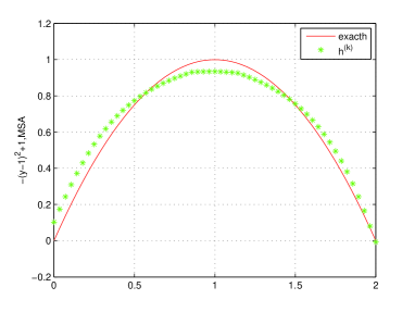
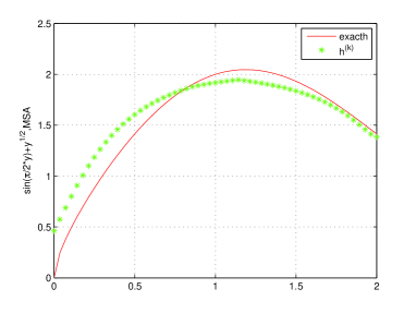
Figure 5.1: Exact and reconstructed fluxes for Examples 5.1 (left) and 5.2 (right)

Table 5.1: Iterative numbers $k$ of MSA and ASA

Algorithm	N	M	$\beta$	error	k
MSA	14	28	0.0001	0.0597	8
	28	56	0.0001	0.0783	8
	56	112	0.0001	0.0907	8
ASA	14	28	0.0001	0.0840	13
	28	56	0.0001	0.0978	13
	56	112	0.0001	0.0959	14

Example 5.2

We take the exact flux $h=\sin(\frac{\pi}{2}y)+y^{\frac{1}{2}}$ on $\Gamma_{1}$, the noise level $\delta=5\%$ and the constant initial guess $h^{(0)}=2$.

Figure 5.1 (right) shows the exact parameter and the numerically recovered parameter, while Table 5.2 gives the number of iterations by Algorithms 3.1 (MSA) and 3.2 (ASA).

Table 5.2: Iterative numbers $k$ of MSA and ASA

Algorithm	N	M	$\beta$	error	k
MSA	14	28	0.0001	0.0827	9
	28	56	0.0001	0.0995	10
	56	112	0.0001	0.0996	11
ASA	14	28	0.0001	0.0981	14
	28	56	0.0001	0.0970	16
	56	112	0.0001	0.0921	15

We can see from Figure 5.1 that the numerical reconstructed fluxes, with a $5\%$ noise in the data, appear to be quite satisfactory, in view of the severe ill-posedness of the inverse flux problem. More importantly, we observe from Tables 5.1 and 5.2 that the convergence of the DD algorithms are nearly optimal with the refinement of the finite element mesh, i.e., the number of iterations grows very mildly with the mesh refinement.

Next, we demonstrate three numerical examples of reconstructing the source strength $f({\bf x})$ in the system (2.1), with $a({\bf x})=(x+y)/100$, $c({\bf x})=1$ in $\Omega$ and $g({\bf x})=0$ on $\partial\Omega$. We start with a constant initial guess $f^{(0)}=0$ in $\Omega$.

Example 5.3

We take the exact source strength $f(x,y)=\sin(2\pi x)\sin(2\pi y)$ and the noise level $\delta=1\%$.

Figure 5.2 shows the exact and numerically recovered source strengths, while Table 5.3 gives the number of iterations by Algorithms 2.1 (MSA) and 2.2 (ASA).

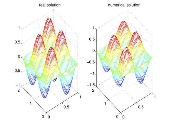
Figure 5.2: Exact and numerically recovered source strengths for Example 5.3

Table 5.3: Number of iterations of Algorithms 2.1 (MSA) and 2.2 (ASA)

Algorithm	N	M	$\beta$	error	k
MSA	7	14	0.001	0.0900	10
	14	28	0.001	0.0971	14
	28	56	0.001	0.0998	14
	56	112	0.001	0.0979	15
ASA	7	14	0.001	0.0956	21
	14	28	0.001	0.0982	30
	28	56	0.001	0.0984	31
	56	112	0.001	0.0991	32

Example 5.4

We take the exact source strength $f=2\sin(2\pi x)y(y-1)(y-2)$ and the noise level $\delta=1\%$.

Figure 5.3 shows the exact and numerically recovered source strengths, while Table 5.4 gives the number of iterations by Algorithms 2.1 (MSA) and 2.2 (ASA).

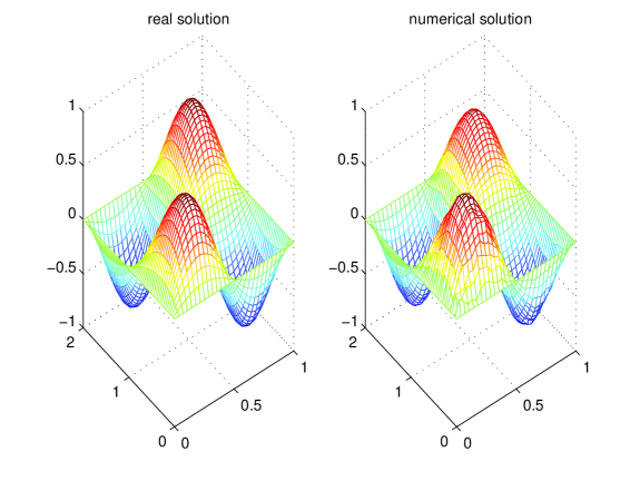
Figure 5.3: Exact and numerically recovered source strengths for Example 5.4

Table 5.4: Number of iterations for Algorithms 2.1 (MSA) and 2.2 (ASA)

Algorithm	N	M	$\beta$	error	k
MSA	7	14	0.001	0.0933	6
	14	28	0.001	0.0991	7
	28	56	0.001	0.0895	8
	56	112	0.001	0.0970	8
ASA	7	14	0.001	0.0100	13
	14	28	0.001	0.0982	16
	28	56	0.001	0.0997	16
	56	112	0.001	0.0959	18

Example 5.5

We take the exact source strength $f(x,y)=10y\sin(2\pi y)x(x-1/2)(x-1)$ and the noise level $\delta=0.01$.

Figure 5.4 shows the exact and numerically recovered source strengths, while Table 5.5 gives the number of iterations by Algorithms 2.1 (MSA) and 2.2 (ASA).

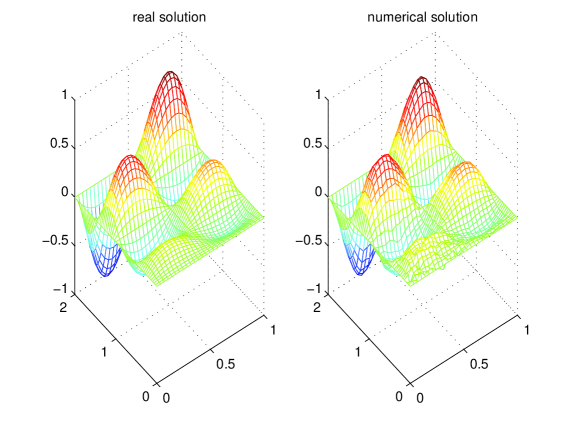
Figure 5.4: Exact and numerically recovered source strengths for Example 5.5

Table 5.5: Number of iterations for Algorithms 2.1 (MSA) and 2.2 (ASA)

Type	N	M	$\beta$	error	k
MSA	7	14	0.001	0.0989	14
	14	28	0.001	0.0976	23
	28	56	0.001	0.0975	24
	56	112	0.001	0.0980	26
ASA	7	14	0.001	0.0977	30
	14	28	0.001	0.0989	47
	28	56	0.001	0.0997	48
	56	112	0.001	0.0999	52

We can see from Figures 5.2-5.4 that the numerical reconstructed source strengths, with a $1\%$ noise in the data, appear to be quite satisfactory, in view of the severe ill-posedness of the inverse source problem and the complicated profiles of the exact source strengths, especially in Example 5.3 where the source strength oscillates frequently between 8 peaks and valleys. More importantly, we observe from Tables 5.3-5.5 that the convergence of the DD algorithms are nearly optimal with the refinement of the finite element mesh, i.e., the number of iterations grows only mildly with the mesh refinement.

Finally, we present three numerical examples for the reconstructions of the initial temperature in the heat conductive system (4.1), by two DD algorithms, namely Algorithms 4.1 and 4.2 proposed in Section 4. In our experiments, we take $a({\bf x})=1$, $f({\bf x},t)=0$, the terminal time $T=4$, with the constant initial guess $\varphi^{(0)}=0$.

Example 5.6

We take the exact initial temperature $\varphi=\sin(2\pi x)\sin(2\pi y)$ and the noise level $\delta=2\%$.

Figure 5.5 shows the exact and numerically recovered initial temperatures, while Table 5.6 gives the number of iterations by Algorithms 4.1 (MSA) and 4.2 (ASA).

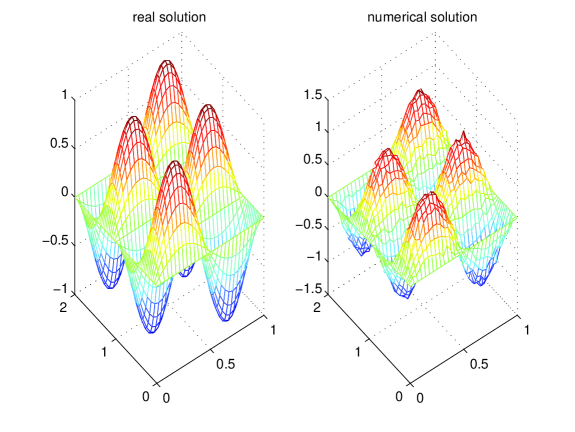
Figure 5.5: Exact and numerically recovered initial temperatures for Example 5.6

Table 5.6: Number of iterations for Algorithms 4.1 (MSA) and 4.2 (ASA)

Algorithm	N	M	$\beta$	error	k
MSA	7	14	0.00005	0.0521	10
	14	28	0.00005	0.0760	11
	28	56	0.00005	0.0998	12
ASA	7	14	0.00005	0.0856	16
	14	28	0.00005	0.0950	20
	28	56	0.00005	0.0973	25

Example 5.7

We take the exact initial temperature $\varphi=2\sin(2\pi x)y(y-1)(y-2)$ and the noise level $\delta=1\%$.

Figure 5.6 shows the exact and numerically recovered initial temperatures, while Table 5.7 gives the number of iterations by Algorithms 4.1 (MSA) and 4.2 (ASA).

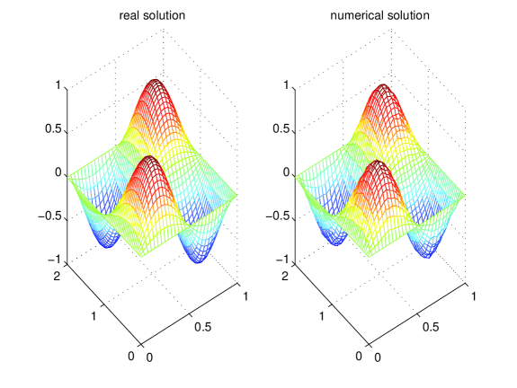
Figure 5.6: Exact and numerically recovered initial temperatures for Example 5.7

Table 5.7: Number of iterations of Algorithms 4.1 (MSA) and 4.2 (ASA)

Algorithm	N	M	$\beta$	error	k
MSA	7	14	0.00005	0.0943	22
	14	28	0.00005	0.0931	26
	28	56	0.00005	0.0995	29
ASA	7	14	0.00005	0.0974	45
	14	28	0.00005	0.0997	52
	28	56	0.00005	0.0971	58

Example 5.8

We take the exact initial temperature $\varphi=10y\sin(2\pi y)x(x-1/2)(x-1)$ and the noise level $\delta=2\%$.

Figure 5.7 shows the exact and numerically recovered initial temperatures, while Table 5.8 gives the number of iterations by Algorithms 4.1 (MSA) and 4.2 (ASA).

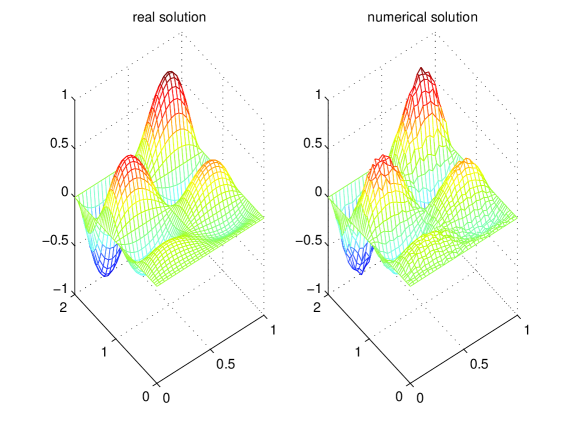
Figure 5.7: Exact and numerically recovered initial temperatures for Example 5.8

Table 5.8: Number of iterations for Algorithms 4.1 (MSA) and 4.2 (ASA)

Algorithm	N	M	$\beta$	error	k
MSA	7	14	0.00005	0.0933	8
	14	28	0.00005	0.0956	10
	28	56	0.00005	0.0989	15
ASA	7	14	0.00005	0.0988	17
	14	28	0.00005	0.0970	22
	28	56	0.00005	0.0993	30

We can see from Figures 5.5-5.7 that the numerical reconstructed initial temperatures, with a $1\%$ noise in the data, appear to be quite satisfactory, in view of the severe ill-posedness of the inverse initial temperature problem and the complicated profiles of the exact initial temperatures, especially in Example 5.6 where the initial temperature oscillates frequently between 8 peaks and valleys. More importantly, we observe from Tables 5.6-5.8 that the convergence of the DD algorithms are nearly optimal with the refinement of the finite element mesh, i.e., the number of iterations grows still mildly with the mesh refinement. But compared with the numerical results for the source strengths and fluxes, we can see that the performance of the reconstructions for the initial temperatures are less satisfactory in terms of the mesh refinement.

6 Concluding remarks

We have proposed several overlapping domain decomposition algorithms for solving some representative linear inverse problems, including the identification of the fluxes, the source intensity and the initial temperature in second order elliptic and parabolic systems. The algorithms are constructed in a way that only small sub-minimizations are needed to solve on the subdomains of the original global domain at each iteration. And it is important to observe from many numerical examples that the convergence of the DD algorithms are nearly optimal with the refinement of the finite element mesh, i.e., the number of iterations grows only mildly with the mesh refinement.

Our future work includes the extension of the proposed overlapping domain decomposition algorithms to nonlinear inverse problems, such as the constructions of the diffusivity coefficient, the radiative coefficient and Robin coefficient in elliptic and parabolic systems.

References

- [1] R.C. Aster, B. Borchers and C.H. Thurber, Parameter Estimation and Inverse Problems, Elsevier Academic Press, New York, 2005.
- [2] H.T. Banks and K. Kunisch, Estimation Techniques for Distributed Parameter Systems, Birkhauser, Boston, 1989.
- [3] X.-C. Cai, S Liu and J. Zou, Parallel overlapping domain decomposition methods for coupled inverse elliptic problems, Comm. Appl. Math. Comput. Sci., 4 (2009), 1-26.
- [4] T.F. Chan and T.P. Mathew, Domain decomposition algorithms, Acta Numerica, (1994), 61-143.
- [5] T.F. Chan and X.C. Tai, Identification of discontinuous coefficients from elliptic problems using total variation regularization, SIAM J. Sci. Comput., 25 (2003), 881-904.
- [6] I. Daubechies, M. Defrise, and C. DeMol, An iterative thresholding algorithm for linear inverse problems, Comm. Pure Appl. Math. 57 (2004), no. 11, 1413-1457.
- [7] H. W. Engl, M. Hanke and A. Neubauer, Regularization of Inverse Problems, Kluwer Academic Publishers, The Netherlands, 2000.
- [8] K. Ito and J. Zou, Identification of some source densities of the distribution type, J. Comput. Appl. Math. 132 (2001), 295-308.
- [9] J.Z. Li and J. Zou, A multilevel model correction method for parameter identification, Inverse Problems 23 (2007), 1759-1786.
- [10] X.C. Tai, J. Froyen, M.S. Espedal and T.F. Chan, Overlapping Domain Decomposition and Multigrid Methods for Inverse Problems, Contemporary Mathematics, 218 (1998), 523-529.
- [11] A. Toselli and O. Widlund, Domain Decomposition Methods - Algorithms and Theory, Springer-Verlag, New York, 2004.
- [12] J. Xie and J. Zou, Numerical reconstruction of heat fluxes, SIAM J. Numer. Anal. 43 (2005) 1504-35.
- [13] J. Xu, Iterative methods by space decomposition and subspace correction, SIAM Review, 34 (1992), 581-613.
- [14] J. Xu and J. Zou, Some nonoverlapping domain decomposition methods, SIAM Review, 40 (1998), 857-914.