Aggregate-Max Nearest Neighbor Searching in the Plane

Abstract

We study the aggregate/group nearest neighbor searching for the Max operator in the plane. For a set $P$ of $n$ points and a query set $Q$ of $m$ points, the query asks for a point of $P$ whose maximum distance to the points in $Q$ is minimized. We present data structures for answering such queries for both $L_{1}$ and $L_{2}$ distance measures. Previously, only heuristic and approximation algorithms were given for both versions. For the $L_{1}$ version, we build a data structure of $O(n)$ size in $O(n\log n)$ time, such that each query can be answered in $O(m+\log n)$ time. For the $L_{2}$ version, we build a data structure in $O(n\log n)$ time and $O(n\log\log n)$ space, such that each query can be answered in $O(m\sqrt{n}\log^{O(1)}n)$ time, and alternatively, we build a data structure in $O(n^{2+\epsilon})$ time and space for any $\epsilon>0$, such that each query can be answered in $O(m\log n)$ time. Further, we extend our result for the $L_{1}$ version to the top-$k$ queries where each query asks for the $k$ points of $P$ whose maximum distances to $Q$ are the smallest for any $k$ with $1\leq k\leq n$: We build a data structure of $O(n)$ size in $O(n\log n)$ time, such that each top-$k$ query can be answered in $O(m+k\log n)$ time.

1 Introduction

Aggregate nearest neighbor (ANN) searching [1, 11, 12, 13, 14, 15, 19, 20, 21, 22, 23], also called group nearest neighbor searching, is a generalization of the fundamental nearest neighbor searching problem [2], where the input of each query is a set of points and the result of the query is based on applying some aggregate operator (e.g., Max and Sum) on all query points. In this paper, we consider the ANN searching on the Max operator for both $L_{1}$ and $L_{2}$ metrics in the plane.

For any two points $p$ and $q$, let $d(p,q)$ denote the distance between $p$ and $q$. Let $P$ be a set of $n$ points in the plane. Given any query set $Q$ of $m$ points, the ANN query asks for a point $p$ in $P$ such that $g(p,Q)$ is minimized, where $g(p,Q)$ is the aggregate function of the distances from $p$ to the points of $Q$. The aggregate functions commonly considered are Max, i.e., $g(p,Q)=\max_{q\in Q}d(p,q)$, and Sum, i.e., $g(p,Q)=\sum_{q\in Q}d(p,q)$. If the operator for $g$ is Max (resp., Sum), we use ANN-Max (resp., ANN-Sum) to denote the problem.

In this paper, we focus on ANN-Max in the plane for both $L_{1}$ and $L_{2}$ versions where the distance $d(p,q)$ is measured by $L_{1}$ and $L_{2}$ metrics, respectively.

Previously, only heuristic and approximation algorithms were given for both versions. For the $L_{1}$ version, we build a data structure of $O(n)$ size in $O(n\log n)$ time, such that each query can be answered in $O(m+\log n)$ time. For the $L_{2}$ version, we build a data structure in $O(n\log n)$ time and $O(n\log\log n)$ space, such that each query can be answered in $O(m\sqrt{n}\log^{O(1)}n)$ time, and alternatively, we build a data structure in $O(n^{2+\epsilon})$ time and space for any $\epsilon>0$, such that each query can be answered in $O(m\log n)$ time.

Furthermore, we extend our result for the $L_{1}$ version to the following ANN-Max top-$k$ queries. In addition to a query set $Q$, each top-$k$ query is also given an integer $k$ with $1\leq k\leq n$, and the query asks for the $k$ points $p$ of $P$ whose values $g(p,Q)$ are the smallest. We build a data structure of $O(n)$ size in $O(n\log n)$ time, such that each $L_{1}$ ANN-Max top-$k$ query can be answered in $O(m+k\log n)$ time.

1.1 Previous Work

For ANN-Max, Papadias et al. [20] presented a heuristic Minimum Bounding Method with worst case query time $O(n+m)$ for the $L_{2}$ version. Recently, Li et al. [11] gave more results on the $L_{2}$ ANN-Max (the queries were called group enclosing queries). By using $R$-tree [8], Li et al. [11] gave an exact algorithm to answer ANN-Max queries, and the algorithm is very fast in practice but theoretically the worst case query time is still $O(n+m)$. Li et al. [11] also gave a $\sqrt{2}$-approximation algorithm with query time $O(m+\log n)$ and the algorithm works for any fixed dimensions, and they further extended the algorithm to obtain a $(1+\epsilon)$-approximation result. To the best of our knowledge, we are not aware of any previous work that is particularly for the $L_{1}$ ANN-Max. However, Li et al. [13] proposed the flexible ANN queries, which extend the classical ANN queries, and they provided an $(1+2\sqrt{2})$-approximation algorithm that works for any metric space in any fixed dimension.

For ANN-Sum, a $3$-approximation solution is given in [13] for the $L_{2}$ version. Agarwal et al. [1] studied nearest neighbor searching under uncertainty, and their results can give an $(1+\epsilon)$-approximation solution for the $L_{2}$ ANN-Sum queries. They [1] also gave an exact algorithm that can solve the $L_{1}$ ANN-Sum problem and an improvement based on their work has been made in [22].

There are also other heuristic algorithms on ANN queries, e.g., [12, 14, 15, 19, 21, 23].

Comparing with $n$, the value $m$ is relative small in practice. Ideally we want a solution that has a query time $o(n)$. Our $L_{1}$ ANN-Max solution is the first-known exact solution and is likely to be the best-possible. Comparing with the heuristic result [11, 20] with $O(m+n)$ worst case query time, our $L_{2}$ ANN-Max solution use $o(n)$ query time for small $m$; it should be noted that the methods in [11, 20] uses only $O(n)$ space while the space used in our approach is larger.

In the following, we give our algorithm for the $L_{1}$ ANN-Max queries in Section 2 and its extension to the top-$k$ is also given in the same section. Our result for the $L_{2}$ metric is presented in Section 3.

2 The ANN-Max in the $L_{1}$ Metric

In this section, we present our solution for the $L_{1}$ version of ANN-Max queries as well as its extension to the top-$k$ queries. We first focus on the ANN-Max queries. Given any query point set $Q$, our goal is to find the point $p\in P$ such that $g(p,Q)=\max_{q\in Q}d(p,q)$ is minimized for the $L_{1}$ distance $d(p,q)$, and we denote by $\psi(Q)$ the above sought point.

For each point $p$ in the plane, denote by $p_{\max}$ the farthest point of $Q$ to $p$. We show below that $p_{\max}$ must be an extreme point of $Q$ along one of the four diagonal directions: northeast, northwest, southwest, southeast.

Figure 1: Illustrating the four extreme points $q_{1},q_{2},q_{3},q_{4}$.

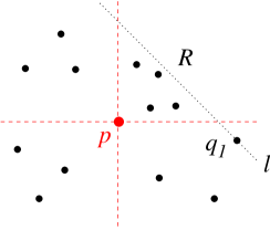
Figure 2: Illustrating the proof for Lemma 1: $Q$ consists of all points except $p$ and $q_{1}$ is in the fourth quadrant.

Let $\rho_{1}$ be a ray directed to the “northeast”, i.e., the angle between $\rho$ and the $x$-axis is $\pi/4$. Let $q_{1}$ be an extreme point of $Q$ along $\rho_{1}$ (e.g., see Fig. 2); if there is more than one such point, we let $q_{1}$ be an arbitrary such point. Similarly, let $q_{2}$, $q_{3}$, and $q_{4}$ be the extreme points along the directions northwest, southwest, and southeast, respectively. Let $Q_{\max}=\{q_{1},q_{2},q_{3},q_{4}\}$. Note that $Q_{\max}$ may have less than four distinct points if two or more points of $Q_{\max}$ refer to the same (physical) point of $Q$. The following lemma shows that $g(p,Q)$ is determined only by the points of $Q_{\max}$.

Lemma 1

For any point $p$ in the plane, $g(p,Q)=\max_{q\in Q_{\max}}d(p,q)$ holds.

Proof: Let $p$ be any point in the plane. If $p_{max}\in Q_{\max}$, the lemma simply follows, otherwise, we show below that there exists a point $q^{\prime}\in Q_{\max}$ such that $d(p,q^{\prime})\geq d(p,p_{\max})$, which proves the lemma.

The vertical line and horizontal line through the point $p$ partition the plane into four quadrants. Without loss of generality, we assume $p_{\max}$ is in the first quadrant (i.e., the northeast quadrant) including its boundary, and we denote the quadrant by $R$. Recall that $q_{1}\in Q_{\max}$ is an extreme point of $Q$ along the northeast direction. Depending on whether $q_{1}\in R$, there are two cases.

1. If $q_{1}\in R$, since $q_{1}$ is an extreme point of $Q$ along the northeast direction, we have $d(p,q_{1})=\max_{q\in Q\cap R}d(p,q)$. Due to $p_{max}\in Q\cap R$, $d(p,q_{1})\geq d(p,p_{\max})$ holds.

2. If $q_{1}\not\in R$, then since $p_{\max}$ is in $R$, by the definition of $q_{1}$, $q_{1}$ is either in the second quadrant or in the fourth quadrant. Without loss of generality, we assume $q_{1}$ is in the fourth quadrant (e.g., see Fig. 2).

   Let $l$ be the line through $q_{1}$ with slope $-1$ and denote by $s$ the line segment that is the intersection of $l$ and $R$. According to the definition of the $L_{1}$ distance measure, all points on $s$ have the same $L_{1}$ distance to $p$, and we denote by $d(p,s)$ the $L_{1}$ distance between $p$ and any point on $s$. Since $q_{1}$ is an extreme point of $Q$ along the northeast direction, all points of $Q$ are below or on the line $l$. This implies $d(p,s)\geq d(p,q)$ for any $q\in Q\cap R$, and in particular, $d(p,s)\geq d(p,p_{\max})$. On the other hand, $q_{1}$ is on $l$ and $q_{1}\not\in R$, we have $d(p,q_{1})\geq d(p,s)$. Hence, we obtain $d(p,q_{1})\geq d(p,p_{\max})$.

The lemma thus follows. $\Box$

Based on Lemma 1, for any point $p$ in the plane, to determine $g(p,Q)$, we only need to consider the points in $Q_{\max}$. Note that a point may have more than one farthest point in $Q$. If $p$ has only one farthest point in $Q$, then $p_{\max}$ is in $Q_{\max}$. Otherwise, $p_{\max}$ may not be in $Q_{\max}$, and for convenience we re-define $p_{\max}$ to be the farthest point of $p$ in $Q_{\max}$.

For each $1\leq i\leq 4$, let $P_{i}=\{p\ |\ p_{\max}=q_{i},p\in P\}$, i.e., $P_{i}$ consists of the points of $P$ whose farthest points in $Q$ are $q_{i}$, and let $p_{i}$ be the nearest point of $q_{i}$ in $P_{i}$. To find $\psi(Q)$, we have the following lemma.

Lemma 2

$\psi(Q)$ is the point $p_{j}$ for some $j$ with $1\leq j\leq 4$, such that $d(p_{j},q_{j})\leq d(p_{i},q_{i})$ holds for any $1\leq i\leq 4$.

Proof: Recall that $\psi(Q)$ is the point $p\in P$ such that the value $g(p,Q)=\max_{q\in Q}d(p,q)$ is minimized. By their definitions, we have the following:

$$\begin{split}\min_{p\in P}g(p,Q)=\min_{p\in P}\max_{q\in Q}d(p,q)=\min_{1\leq i\leq 4}\{\min_{p\in P_{i}}\max_{q\in Q}d(p,q)\}=\min_{1\leq i\leq 4}\{\min_{p\in P_{i}}d(p,q_{i})\}=\min_{1\leq i\leq 4}\{d(p_{i},q_{i})\}.\end{split}$$

The lemma thus follows. $\Box$

Based on Lemma 2, to determine $\psi(Q)$, it is sufficient to determine $p_{i}$ for each $1\leq i\leq 4$. To this end, we make use of the farthest Voronoi diagram [6] of the four points in $Q_{\max}$, which is also the farthest Voronoi diagram of $Q$ by Lemma 1. Denote by $\mbox{$F\!V\!D$}(Q)$ the farthest Voronoi diagram of $Q_{\max}$. Since $Q_{\max}$ has only four points, $\mbox{$F\!V\!D$}(Q)$ can be computed in constant time, e.g., by an incremental approach. Each point $q\in Q_{\max}$ defines a cell $C(q)$ in $\mbox{$F\!V\!D$}(Q)$ such that every point $p\in C(q)$ is farthest to $q_{i}$ among all points of $Q_{\max}$. In order to compute the four points $p_{i}$ with $i=1,2,3,4$, we first show in the following that each cell $C(q)$ has certain special shapes that allow us to make use of the segment dragging queries [5, 18] to find the four points efficiently. Note that for each $1\leq i\leq 4$, $P_{i}=P\cap C(q_{i})$ and thus $p_{i}$ is the nearest point of $P\cap C(q_{i})$ to $q_{i}$. In fact, the following discussion also gives an incremental algorithm to compute $\mbox{$F\!V\!D$}(Q)$ in constant time.

2.1 The Bisectors

We first briefly discuss the bisectors of the points based on the $L_{1}$ metric. In fact, the $L_{1}$ bisectors have been well studied (e.g., [18]) and we discuss them here for completeness and some notation introduced here will also be useful later when we describe our algorithm.

For any two points $q$ and $q^{\prime}$ in the plane, define $r(q,q^{\prime})$ as the region of the plane that is the locus of the points farther to $q$ than to $q^{\prime}$, i.e., $r(q,q^{\prime})=\{p\ |\ d(p,q)\geq d(p,q^{\prime})\}$. The bisector of $q$ and $q^{\prime}$, denoted by $B(q,q^{\prime})$, is the locus of the points that are equidistant to $q$ and $q^{\prime}$, i.e., $B(q,q^{\prime})=\{p\ |\ d(p,q)=d(p,q^{\prime})\}$. In order to discuss the shapes of the cells of $\mbox{$F\!V\!D$}(Q)$, we need to elaborate on the shape of $B(q,q^{\prime})$, as follows.

Let $R(q,q^{\prime})$ be the rectangle that has $q$ and $q^{\prime}$ as its two vertices on diagonal positions (e.g., see Fig. 3). In the special case where the line segment $\overline{qq^{\prime}}$ is axis-parallel, the rectangle $R(q,q^{\prime})$ is degenerated into a line segment and $B(q,q^{\prime})$ is the line through the midpoint of $\overline{qq^{\prime}}$ and perpendicular to $\overline{qq^{\prime}}$. Below, we focus on the general case where $\overline{qq^{\prime}}$ is not axis-parallel. Without loss of generality, we assume $q$ and $q^{\prime}$ are northeast and southwest vertices of $R(q,q^{\prime})$, and other cases are similar.

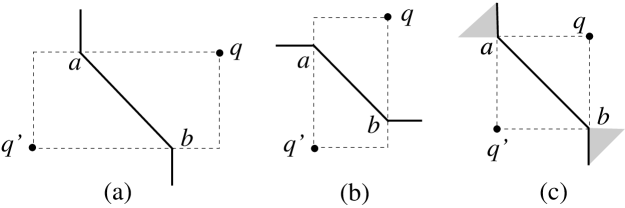
Figure 3: Illustrating the bisector $B(q,q^{\prime})$ (the solid curve) for $q$ and $q^{\prime}$. In (c), since $R(q,q^{\prime})$ is a square, the two shaded quadrants are entirely in $B(q,q^{\prime})$, but for simplicity, we only consider the two vertical bounding half-lines as in $B(q,q^{\prime})$.

The bisector $B(q,q^{\prime})$ consists of two half-lines and one line segment in between (e.g., see Fig. 3); the two half-lines are either both horizontal or both vertical. More specifically, let $l$ be the line of slope $-1$ that contains the midpoint of $\overline{qq^{\prime}}$. Let $\overline{ab}=l\cap R(q,q^{\prime})$, and $a$ and $b$ are on the boundary of $R(q,q^{\prime})$. Note that if $R(q,q^{\prime})$ is a square, then $a$ and $b$ are the other two vertices of $R(q,q^{\prime})$ than $q$ and $q^{\prime}$; otherwise, neither $a$ nor $b$ is a vertex.

We first discuss the case where $R(q,q^{\prime})$ is not a square (e.g., see Fig. 3 (a) and (b)). Let $l(a)$ be the line through $a$ and perpendicular to the edge of $R(q,q^{\prime})$ that contains $a$. The point $a$ divides $l(a)$ into two half-lines, and we let $l^{\prime}(a)$ be the one that doest not intersect $R(q,q^{\prime})$ except $a$. Similarly, we define the half-line $l^{\prime}(b)$. Note that $l^{\prime}(a)$ and $l^{\prime}(b)$ must be parallel. The bisector $B(q,q^{\prime})$ is the union of $l^{\prime}(a)$, $\overline{ab}$, and $l^{\prime}(b)$.

If $R(q,q^{\prime})$ is a square, then $a$ and $b$ are both vertices of $R(q,q^{\prime})$ (e.g., see Fig. 3 (c)). In this case, a quadrant of $a$ and a quadrant of $b$ belong to the bisector $B(q,q^{\prime})$, but for simplicity, we consider $B(q,q^{\prime})$ as the union of $\overline{ab}$ and the two vertical bounding half-lines of the two quadrants.

We call $\overline{ab}$ the middle segment of $B(q,q^{\prime})$ and denote it by $B_{M}(q,q^{\prime})$. If $B(q,q^{\prime})$ contains two vertical half-lines, we call $B(q,q^{\prime})$ a v-bisector and refer to the two half-lines as upper half-line and lower half-line, respectively, based on their relative positions; similarly, if $B(q,q^{\prime})$ contains two horizontal half-lines, we call $B(q,q^{\prime})$ an h-bisector and refer to the two half-lines as left half-line and right half-line, respectively.

For any point $p$ in the plane, we use $l^{+}(q)$ to denote the line through $q$ with slope $1$, $l^{-}(q)$ the line through $q$ with slope $-1$, $l_{h}(q)$ the horizontal line through $q$, and $l_{v}(q)$ the vertical line through $q$.

2.2 The Shapes of Cells of $\mbox{$F\!V\!D$}(Q)$

In the following, we discuss the shapes of the cells of $\mbox{$F\!V\!D$}(Q)$. A subset $Q^{\prime}$ of $Q$ is extreme if it contains an extreme point along each of the four diagonal directions. The set $Q_{\max}$ is an extreme subset. A point $q$ of $Q_{\max}$ is redundant if $Q_{\max}\setminus\{q\}$ is still an extreme subset. For simplicity of discussion, we remove all redundant points from $Q_{\max}$. For example, if $q_{1}$ and $q_{2}$ are both extreme points along the northeast direction (and $q_{2}$ is also an extreme point along the northwest direction), then $q_{1}$ is redundant and we simply remove $q_{1}$ from $Q_{\max}$ (and the new $q_{1}$ of $Q_{\max}$ now refers to the same physical point as $q_{2}$).

Consider a point $q\in Q_{\max}$. Without loss of generality, we assume $q=q_{3}$ and the other cases can be analyzed similarly. We will analyze the possible shapes of $C(q_{3})$. We assume $Q_{\max}$ has at least two distinct points since otherwise the problem would be trivial. We further assume $q_{1}\neq q_{3}$ since otherwise the analysis is much simpler. According to their definitions, $q_{1}$ must be above the line $l^{-}(q_{3})$ (e.g., see Fig. 4). However, $q_{1}$ can be either above or below the line $l^{+}(q_{3})$. In the following discussion, we assume $q_{1}$ is below or on the line $l^{+}(q_{3})$ and the case where $q_{1}$ is above $l^{+}(q_{3})$ can be analyzed similarly. In this case $B(q_{3},q_{1})$ is a v-bisector (i.e., it has two vertical half-lines).

Figure 4: Illustrating an example where $q_{1}$ is above $l^{-}(q_{3})$ and below or on $l^{+}(q_{3})$. The bisector $B(q_{1},q_{3})$ is a v-bisector (i.e., it has two vertical half-lines).

We first introduce three types of regions (i.e., type-A, type-B, and type-C), and we will show later that $C(q_{3})$ must belong to one of the types. Each type of region is bounded from the left or below by a polygonal curve $\partial$ consisting of two half-lines and a line segment of slope $\pm 1$ in between (the line segment may be degenerated into a point).

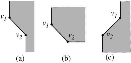
Figure 5: Illustrating three types of regions (shaded).

1. From top to bottom, the polygonal curve $\partial$ consists of a vertical half-line followed by a line segment of slope $-1$ and then followed by a vertical half-line extended downwards (e.g., see Fig. 5 (a)). The region on the right of $\partial$ is defined as a type-A region.

2. From top to bottom, the polygonal curve $\partial$ consists of a vertical half-line followed by a line segment of slope $-1$ and then followed by a horizontal half-line extended rightwards (e.g., see Fig. 5 (b)). The region on the right of and above $\partial$ is defined as a type-B region.

3. From top to bottom, the polygonal curve $\partial$ consists of a vertical half-line followed by a line segment of slope $1$ and then followed by a vertical half-line extended downwards (e.g., see Fig. 5 (c)). The region on the right of $\partial$ is defined as a type-C region.

In each type of the regions, the line segment of $\partial$ is called the middle segment. Denote by $v_{1}$ the upper endpoint of the middle segment and by $v_{2}$ the lower endpoint (e.g., see Fig. 5). Again, the middle segment may be degenerated to a point. The following lemma shows that $C(q_{3})$ must belong to one of the three types of regions.

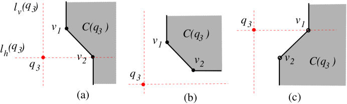
Figure 6: Illustrating the three possible cases for $C(q_{3})$: (a) a type-A region; (b) a type-B region; (c) a type-C region.

Lemma 3

The cell $C(q_{3})$ must be one of the three types of regions. Further (e.g., see Fig. 6), if $C(q_{3})$ is a type-A region, then $C(q_{3})$ is to the right of $l_{v}(q_{3})$ and $v_{2}$ is on $l_{h}(q_{3})$; if $C(q_{3})$ is a type-B region, then $C(q_{3})$ is to the right of $l_{v}(q_{3})$ and above $l_{h}(q_{3})$; if $C(q_{3})$ a type-C region, then $C(q_{3})$ is to the right of $l_{v}(q_{3})$ and $v_{1}$ is on $l_{h}(q_{3})$.

Proof: For any point $q$ in the plane, we use $y(q)$ to denote the $y$-coordinate of $q$ and use $x(q)$ to denote the $x$-coordinate of $q$.

The proof is essentially an incremental approach to construct the cell $C(q_{3})$. We first discuss the case where $y(q_{1})\geq y(q_{3})$ (e.g., see Fig. 8). Consider the bisector $B(q_{1},q_{3})$, which is a v-bisector in this case (i.e., the two half-lines of $B(q_{1},q_{3})$ are vertical).

First of all, if $q_{1}$ and $q_{3}$ are the only distinct points of $Q_{\max}$, then $C(q_{3})$ is $r(q_{3},q_{1})$ and thus $C(q_{3})$ is a type-A region. Further, $C(q_{3})$ is to the right of $l_{v}(q_{3})$ and $v_{2}$ is on $l_{h}(q_{3})$. The lemma thus follows. Below, we assume $q_{2}$ is also distinct and the case where $q_{4}$ is distinct is similar.

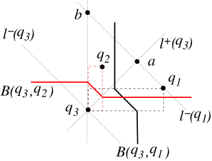
Figure 7: Illustrating the bisector $B(q_{3},q_{1})$ and the intersection $r(q_{3},q_{1})\cap r(q_{3},q_{2})$.

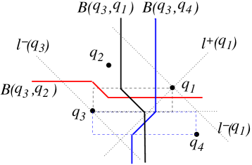
Figure 8: Illustrating the bisector $B(q_{3},q_{4})$ and the intersection $r(q_{3},q_{1})\cap r(q_{3},q_{2})\cap r(q_{3},q_{4})$.

According to their definitions, $q_{2}$ must be above $l^{-}(q_{3})$, below $l^{-}(q_{1})$, and above $l^{+}(q_{3})$ (e.g., see Fig. 8); note that $q_{2}$ cannot be on any of the above three lines since otherwise $Q_{\max}$ would have a redundant point. We analyze the shape of the intersection $r(q_{3},q_{1})\cap r(q_{3},q_{2})$. Let $a$ be the intersection of $l^{+}(q_{3})$ and $l^{-}(q_{1})$. Let $b$ be the intersection of $l_{v}(q_{3})$ and $l^{-}(q_{1})$. Depending on whether $q_{2}$ is in the triangle $\triangle abq_{3}$, there are two cases.

• If $q_{2}\not\in\triangle abq_{3}$, then $x(q_{2})\leq x(q_{3})$. Since $q_{2}$ is above the line $l^{-}(q_{3})$, the bisector $B(q_{3},q_{2})$ is an h-bisector. Since the rectangle $R(q_{3},q_{2})$ is on the left of $l_{v}(q_{3})$ and the bisector $B(q_{3},q_{1})$ is to the right of $l_{v}(q_{3})$, only the right half-line of $B(q_{3},q_{2})$ intersects $B(q_{3},q_{1})$ at a point either on the upper half-line or on the middle segment of $B(q_{3},q_{1})$. In either case, the intersection $r(q_{3},q_{1})\cap r(q_{3},q_{2})$ is a type-B region that is above $l_{h}(q_{3})$ and to the right of $l_{v}(q_{3})$.

• If $q_{3}$ is strictly inside $\triangle abq_{3}$ (e.g., see Fig. 8), then the bisector $B(q_{3},q_{2})$ is an h-bisector and its middle segment $B_{M}(q_{3},q_{2})$ is of slope $-1$. We claim that the line containing $B_{M}(q_{3},q_{2})$ is to the left of the line containing $B_{M}(q_{3},q_{1})$. This can be proved by basic geometric techniques, as follows.

  Since $q_{2}$ is in the interior of $\triangle abq_{3}$, we extend $\overline{q_{3}q_{2}}$ until it hits a point on the segment $\overline{ab}$ and let $q^{\prime}$ be the above point. Since $q^{\prime}$ is on $l^{-}(q_{1})$, the middle segment $B_{M}(q_{3},q^{\prime})$ is exactly on the line containing $B_{M}(q_{3},q_{1})$. Since $x(q_{2})<x(q^{\prime})$, the claim follows.

  The claim implies that the middle segment $B_{M}(q_{3},q_{2})$ does not intersect $B(q_{3},q_{1})$. Since the left horizontal half-line of $B(q_{3},q_{2})$ is on the left of $l_{v}(q_{3})$, it does not intersect $B(q_{3},q_{1})$ either. Hence, only the right horizontal half-line of $B(q_{3},q_{2})$ intersects $B(q_{3},q_{1})$, again at a point on the upper half-line or the middle segment of $B(q_{3},q_{1})$. Therefore, the intersection $r(q_{3},q_{1})\cap r(q_{3},q_{2})$ is a type-B region, which is above $l_{h}(q_{3})$ and to the right of $l_{v}(q_{3})$.

In summary, the intersection $r(q_{3},q_{1})\cap r(q_{3},q_{2})$ is a type-B region that is above $l_{h}(q_{3})$ and to the right of $l_{v}(q_{3})$. If there is no such a distinct point $q_{4}$, we are done with proving the lemma. In the following, we assume there is a distinct point $p_{4}$. Hence, the cell $C(q_{3})$ is $r(q_{3},q_{1})\cap r(q_{3},q_{2})\cap r(q_{3},q_{4})$.

According to their definitions, $q_{4}$ must be below $l^{-}(q_{1})$, above $l^{-}(q_{3})$, and below $l^{+}(q_{1})$ (e.g., see Fig. 8). Note that the bisector $B(q_{3},q_{4})$ must be a v-bisector. Depending on whether $y(q_{4})\leq y(q_{3})$, there are two cases.

• If $y(q_{4})\leq y(q_{3})$ (e.g., see Fig. 8), then each point of the rectangle $R(q_{3},q_{4})$ is below or on the line $l_{h}(q_{3})$. Hence, only the upper vertical line of $B(q_{3},q_{4})$ is possible to intersect $r(q_{3},q_{1})\cap r(q_{3},q_{2})$. Recall that $r(q_{3},q_{1})\cap r(q_{3},q_{2})$ is a type-B region. If the vertical half-line of $B(q_{3},q_{4})$ intersects $r(q_{3},q_{1})\cap r(q_{3},q_{2})$, then the cell $C(q_{3})$, which is $r(q_{3},q_{1})\cap r(q_{3},q_{2})\cap r(q_{3},q_{4})$, is a type-B region, otherwise $C(q_{3})=r(q_{3},q_{1})\cap r(q_{3},q_{2})$ is also a type-B region. In either case, $C(q_{3})$ is above $l_{h}(q_{3})$ and to the right of $l_{v}(q_{3})$. The lemma thus follows.

• If $y(q_{4})>y(q_{3})$, then $q_{4}$ is in the triangle formed by the three lines $l_{h}(q_{3})$, $l^{-}(q_{1})$, and $l^{+}(q_{1})$. The middle segment of $B(q_{3},q_{4})$ is of slope $-1$. We claim that the middle segment $B_{M}(q_{3},q_{4})$ must be in the rectangle $R(q_{3},q_{1})$ and is to the left of the middle segment $B_{M}(q_{3},q_{1})$. Indeed, let $d$ be the intersection of $l_{h}(q_{3})$ and $l^{-}(q_{1})$. Let $e$ be the lower endpoint of $B_{M}(q_{3},q_{1})$. By the definition of the middle segments, $e$ is the midpoint of $\overline{q_{3}d}$. Since the lower edge of $R(q_{3},q_{4})$ is contained in $\overline{q_{3}d}$ and $q_{4}$ is below $l^{-}(q_{1})$, we can obtain the claim above.

  The claim implies that neither the middle segment nor the lower vertical half-line of $B(q_{3},q_{4})$ can intersect $B(q_{3},q_{1})$. Therefore, only the upper vertical half-line of $B(q_{3},q_{4})$ can intersect $r(q_{3},q_{1})\cap r(q_{3},q_{2})$. Therefore, as in the first case, $C(q_{3})$ is a type-B regions that is above $l_{h}(q_{3})$ and to the right of $l_{v}(q_{3})$. The lemma thus follows.

We have proved the lemma for the case where $y(q_{1})\geq y(q_{3})$. Next, we consider the case where $y(q_{1})<y(q_{3})$ (e.g., see Fig. 10). The analysis is similar and we briefly discuss it below.

In this case, the middle segment $B_{M}(q_{3},q_{1})$ is of slope $1$. If there is no other distinct point in $Q_{\max}$, then $C(q_{3})=r(q_{3},q_{1})$ and $C(q_{3})$ is a type-C region that is to the right of $l_{v}(q_{3})$ and $v_{1}$ (i.e., the upper endpoint of the middle segment) is on $l_{h}(v_{3})$, which proves the lemma. Below, we assume $q_{2}$ is another distinct point and the case for $q_{4}$ is similar.

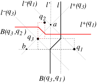
Figure 9: Illustrating the case where $y(q_{1})<y(q_{3})$ and $q_{2}$ is shown.

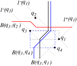
Figure 10: Illustrating the case where $y(q_{1})<y(q_{3})$ and both $q_{2}$ and $q_{4}$ are shown.

Again, $q_{2}$ must be above $l^{-}(q_{3})$, below $l^{-}(q_{1})$, and above $l^{+}(q_{3})$. The bisector $B(q_{3},q_{2})$ is an h-bisector (e.g., see Fig. 10). Let $l$ be the vertical line containing the upper half-line of $B(q_{3},q_{1})$. We claim that $q_{2}$ must be to the left of $l$. To prove the claim, it is sufficient to show that the point $a$ is to the left of $l$, where $a$ is the intersection of $l^{-}(q_{1})$ and $l^{+}(q_{3})$. To this end, we first show that $a$ must be on $l^{\prime}$, where $l^{\prime}$ is the vertical line containing the lower vertical half-line of $B(q_{3},q_{1})$. To see this, consider the triangle $\triangle abq_{1}$ where $b$ is the intersection of $l_{h}(q_{1})$ and $l^{+}(q_{3})$. According to the definition of the middle segment of $B(q_{3},q_{1})$, the lower endpoint of $B_{M}(q_{3},q_{1})$ is the midpoint of $\overline{bq_{1}}$. Further, since $\overline{ab}$ is of slope $1$ and $\overline{aq_{1}}$ is of slope $-1$, the angle $\angle baq_{1}=\pi/2$ and the Euclidean lengths of $\overline{ab}$ and $\overline{aq_{1}}$ are the same. Therefore, $a$ is on $l^{\prime}$. Since $B_{M}(q_{3},q_{1})$ is of slope $1$, $l^{\prime}$ is to the left of $l$. The claim is proved.

Since $q_{2}$ must be above $l_{h}(q_{3})$, the above claim implies that only the right horizontal half-line of $B(q_{3},q_{2})$ intersects $B(q_{3},q_{1})$ and the intersection is on the upper vertical line of $B(q_{3},q_{1})$. Therefore, $r(q_{3},q_{2})\cap r(q_{3},q_{1})$ is a type-B region that is above $l_{h}(q_{3})$ and to the right of $l_{v}(q_{3})$. In fact, $r(q_{3},q_{2})\cap r(q_{3},q_{1})$ is a degenerate type-B region as its boundary consists of a vertical half-line and a horizontal half-line. If there is no such a distinct point $q_{4}$ in $Q_{\max}$, we are done with proving the lemma. In the following, we assume $q_{4}$ is another distinct point, and thus $C(q_{3})=r(q_{3},q_{2})\cap r(q_{3},q_{1})\cap r(q_{3},q_{4})$.

Again, $q_{4}$ must be below $l^{+}(q_{1})$, above $l^{-}(q_{3})$, and below $l^{-}(q_{1})$ (e.g., see Fig. 10). The bisector $B(q_{3},q_{4})$ must be a v-bisector. Since no point of the rectangle $R(q_{3},q_{4})$ is above the line $l_{h}(q_{3})$ and $r(q_{3},q_{2})\cap r(q_{3},q_{1})$ is above $l_{h}(q_{3})$, only the upper vertical line of $B(q_{3},q_{4})$ is possible to intersect $r(q_{3},q_{2})\cap r(q_{3},q_{1})$. Regardless of whether the upper vertical line of $B(q_{3},q_{4})$ intersects $r(q_{3},q_{2})\cap r(q_{3},q_{1})$, $C(q_{3})$ is always a (degenerate) type-B region that is above $l_{h}(q_{1})$ and to the right of $l_{v}(q_{3})$.

The lemma is thus proved. $\Box$

2.3 Answering the Queries

Recall that our goal is to compute $p_{3}$, which is the nearest point of $P\cap C(q_{3})$ to $q_{3}$. Based on Lemma 3, we can compute the point $p_{3}$ in $O(\log n)$ time by making use of the segment dragging queries [5, 18]. The details are given in Lemma 4.

Lemma 4

After $O(n\log n)$ time and $O(n)$ space preprocessing on $P$, the point $p_{3}$ can be found in $O(\log n)$ time.

Proof: Before giving the algorithm, we briefly discuss the segment dragging queries that will be used by our algorithm.

Figure 11: Illustrating the segment dragging queries: (a) a parallel-track query; (b) an out-of-corner query.

Given a set $S$ of $n$ points in the plane, we introduce two types of segment dragging queries: the parallel-track queries and the out-of-corner queries (e.g., Fig. 11). For each parallel-track query, we are given two parallel vertical or horizontal lines (as “tracks”) and a line segment of slope $\pm 1$ with endpoints on the two tracks, and the goal is to find the first point of $S$ hit by the segment if we drag the segment along the two tracks. For each out-of-corner query, we are given two axis-parallel tracks forming a perpendicular corner, and the goal is to find the first point of $S$ hit by dragging out of the corner a segment of slope $\pm 1$ with endpoints on the two tracks.

For the parallel-track queries, as shown by Mitchell [18], we can use Chazelle’s approach [5] to answer each query in $O(\log n)$ time after $O(n\log n)$ time and $O(n)$ space preprocessing on $S$. For the our-of-corner dragging queries, by transforming it to a point location problem, Mitchell [18] gave an algorithm that can answer each query in $O(\log n)$ time after $O(n\log n)$ time and $O(n)$ space preprocessing on $S$.

In the sequel, we present our algorithm for the lemma by using the above segment dragging queries. Our goal is to find $p_{3}$, which is the closest point of $P\cap C(q_{3})$ to $q_{3}$. Depending on the type of the $C(q_{3})$ as stated in Lemma 3, there are three cases.

1. If $C(q_{3})$ is a type-A region, we further decompose $C(q_{3})$ into three subregions (e.g., see Fig. 12 (a)) by introducing two horizontal half-lines going rightwards from $v_{1}$ and $v_{2}$ (i.e., the endpoints of the middle segment of the boundary of $C(q_{3})$), respectively. We call the three subregions the upper, middle, and lower subregions, respectively, according to their heights. To find $p_{3}$, for each subregion $C$, we compute the closest point of $P\cap C$ to $q_{3}$, and $p_{3}$ is the closest point to $q_{3}$ among the three points found above.

   

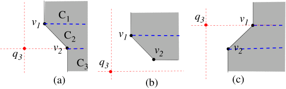
   Figure 12: Illustrating the decomposition of $C(q_{3})$ for segment-dragging queries.

   For the upper subregion, denoted by $C_{1}$, according to Lemma 3, $C_{1}$ is in the first quadrant of $q_{3}$. Therefore, $q_{3}$’s closest point in $P\cap C_{1}$ is exactly the answer of the out-of-corner query by dragging a segment of slope $-1$ from the corner of $C_{1}$.

   For the middle subregion, denoted by $C_{2}$, according to Lemma 3, $C_{2}$ is in the first quadrant of $q_{3}$. Therefore, $q_{3}$’s closest point in $P\cap C_{2}$ is exactly the answer of the parallel-track query by dragging the middle segment of the boundary of $C(q_{3})$ rightwards.

   For the lower subregion, denoted by $C_{3}$, according to Lemma 3, $C_{3}$ is in the fourth quadrant of $q_{3}$. Therefore, $q_{3}$’s closest point in $P\cap C_{3}$ is exactly the answer of the out-of-corner query by dragging a segment of slope $1$ from the corner of $C_{3}$.

   Therefore, in this case we can find $p_{3}$ in $O(\log n)$ time after $O(n\log n)$ time and $O(n)$ space preprocessing on $P$.

2. If $C(q_{3})$ is a type-B region, we further decompose $C(q_{3})$ into two subregions (e.g., see Fig. 12 (b)) by introducing a horizontal half-line rightwards from $v_{1}$. To find $p_{3}$, again, we find the closest point to $q_{3}$ in each of the two sub-regions.

   According to Lemma 3, both subregions are in the first quadrant of $q_{3}$. By using the same approach as the first case, $q_{3}$’s closest point in the upper subregion can be found by an out-of-corner query and $q_{3}$’s closest point in the lower subregion can be found by a parallel-track query.

3. If $C(q_{3})$ is a type-C region, the case is symmetric to the first case and we can find $p_{3}$ by using two out-of-corner queries and a parallel-track query.

As a summary, we can find $p_{3}$ in $O(\log n)$ time after $O(n\log n)$ time $O(n)$ space preprocessing on $P$. The lemma thus follows. $\Box$

By combining Lemmas 2 and 4, we have the following theorem.

Theorem 1

Given a set $P$ of $n$ points in the plane, after $O(n\log n)$ time and $O(n)$ space preprocessing, we can answer each $L_{1}$ ANN-Max query in $O(m+\log n)$ time for any set $Q$ of $m$ query points.

Proof: As preprocessing, we build data structures for answering the segment dragging queries on $P$ [5, 18]. The preprocessing takes $O(n\log n)$ time and $O(n)$ space.

Given any query set $Q$, we first determine $Q_{\max}$ in $O(m)$ time. Then, we compute the farthest Voronoi diagram $\mbox{$F\!V\!D$}(Q)$ in constant time, e.g., by the incremental approach given in this paper. Then, for each $1\leq i\leq 4$, we compute the point $p_{i}$ by Lemma 4 in $O(\log n)$ time. Finally, $\psi(Q)$ can be determined by Lemma 2. $\Box$

2.4 The Top-$k$ Queries

We extend our result in Theorem 1 to the top-$k$ queries. All notations here follow those defined previously. Consider any value $k$ with $1\leq k\leq n$.

For each point $q\in Q_{\max}$, e.g., $q=q_{3}$ as defined earlier, our algorithm will find $k$ points from $P\cap C(q_{3})$ nearest to $q_{3}$ in sorted order by their distances to $q_{3}$. If $|P\cap C(q_{3})|<k$, all points of $P\cap C(q_{3})$ will be reported and no other points will be reported. Due to $|Q_{\max}|\leq 4$, we will obtain at most $4k$ points, and among them the $k$ points with the smallest values $g(p,Q)$ are the sought points for the top-$k$ query, which can be found in additional $O(k)$ time since the above $4k$ points are reported as four sorted lists by their values $g(p,Q)$. The following lemma finds the $k$ points of $P\cap C(q_{3})$ nearest to $q_{3}$ and the algorithms for other points of $Q_{\max}$ are similar.

Lemma 5

After $O(n\log n)$ time and $O(n)$ space preprocessing on $P$, the $k$ points of $P\cap C(q_{3})$ nearest to $q_{3}$ can be found in $O(k\log n)$ time and these points are reported in sorted order by their distances to $q_{3}$.

Proof: We assume $|P\cap C(q_{3})|\geq k$ since the case $|P\cap C(q_{3})|<k$ can be easily solved. For ease of exposition, we also make a general position assumption that no two points of $P$ lie on the same line of slope $1$ or $-1$, and our approach can be generalized to handle the general case.

We follow the discussion in the proof of Lemma 4. As preprocessing, we build the segment-dragging query data structures [5, 18], which takes $O(n\log n)$ time and $O(n)$ space. Recall that the shape of the cell $C(q_{3})$ has three types. We assume $C(q_{3})$ is a type-A and the other two types can be handled analogously. Let $p^{\prime}_{1},p_{2}^{\prime},\ldots,p_{k}^{\prime}$ be the $k$ points of $P\cap C(q_{3})$ nearest to $q_{3}$ in the increasing order by their distances to $q_{3}$, and our algorithm will report them in this order.

Recall that to find $p_{1}^{\prime}$, we partition $C(q_{3})$ into three subregions $C_{1}$, $C_{2}$, and $C_{3}$, and for each subregion $C$, we find the nearest point of $P\cap C$ to $q_{3}$; we call the above point the candidate point for $p_{1}^{\prime}$. Let $H$ denote the set of the above three candidate points. The point of $H$ nearest to $q_{3}$ is $p_{1}^{\prime}$. Below we discuss how to find $p_{2}^{\prime}$.

We first remove $p_{1}^{\prime}$ from $H$. Next, we will find three new candidate points and insert them to $H$, such that $p_{2}^{\prime}$ is the nearest point of $H$ to $q_{3}$. The details are given below. Depending on which subregion of $C(q_{3})$ the point $p_{1}^{\prime}$ belongs to, there are three cases.

1. If $p_{1}^{\prime}\in C_{1}$, let $p$ be the second nearest point of $P\cap C_{1}$ to $q_{3}$. It is easy to see that $p_{2}^{\prime}$ must be one of the points in $H\cup\{p\}$. Recall that $p_{1}^{\prime}$ is found by dragging a segment $s$ of slope $-1$ out of the corner of $C_{1}$ (i.e., $v_{1}$, see Fig. 12). After $s$ hits $p_{1}^{\prime}$, if we keep dragging $s$, $p$ is the next point that will be hit by $s$. To find $p$, unfortunately we cannot use the same out-of-corner segment dragging query data structure [18] because the data structure only works when the triangle formed by $v_{1}$ and $s$ does not contain any point in its interior (see [18] for more details on this). Instead, we use the following approach.

   

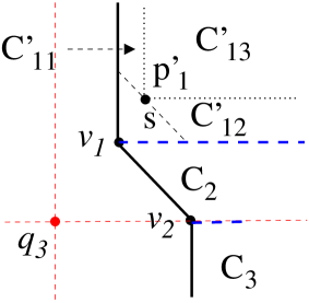
   Figure 13: Partitioning $C_{1}^{\prime}$ into three regions: $C^{\prime}_{11}$, $C^{\prime}_{12}$, and $C^{\prime}_{13}$.

   At the moment $s$ hits $p_{1}^{\prime}$, let $C^{\prime}_{1}$ be the subset of $C_{1}$ to the right and above of $s$, i.e., $C^{\prime}_{1}$ is $C_{1}$ excluding the triangle formed by $v_{1}$ and $s$ (e.g., see Fig. 13). We partition $C^{\prime}_{1}$ into three subregions in the following way (e.g., see Fig. 13). Let $C_{11}^{\prime}$ be the region of $C^{\prime}_{1}$ on the left of the vertical line through $q_{3}$. Let $C_{12}^{\prime}$ be the region of $C^{\prime}_{1}$ below the horizontal line through $q_{3}$. Let $C_{13}^{\prime}$ be the remaining part of $C^{\prime}_{1}$. For simplicity of discussion, we assume the region $C_{i1}^{\prime}$ does not contain the point $p_{1}^{\prime}$ for any $1\leq i\leq 3$.

   Denote by $p^{\prime\prime}_{i}$ the nearest point to $q_{3}$ in $P\cap C_{1i}^{\prime}$, for each $1\leq i\leq 3$. Hence, one of $p^{\prime\prime}_{i}$ for $i=1,2,3$ must be $p$, i.e., the second nearest point of $P\cup C_{1}$ to $q_{3}$. We insert the above three points to $H$, and consequently, $p_{2}^{\prime}$ is the point of $H$ nearest to $q_{3}$. It remains to find the above three points.

   The point $p_{1}^{\prime}$ partitions $s$ into two sub-segments: let $s_{1}$ be the sub-segment bounding $C^{\prime}_{11}$ and $s_{2}$ be the one bounding $C^{\prime}_{12}$. The point $p_{1}^{\prime\prime}$ can be found by a parallel-track segment dragging query by dragging the segment $s_{1}$ upwards. However, there is an issue for the approach. Since $p_{1}^{\prime}$ is an endpoint of $s_{1}$, the above query may still return $p_{1}^{\prime}$ as the answer. We use a little trick to get around the issue. Due to our general position assumption that no two points lie on the same line of slope $\pm 1$, $s_{1}$ does not contain any other point of $P$ than $p_{1}^{\prime}$. Instead of dragging $s_{1}$, we drag another segment $s_{1}^{\prime}$ which can be viewed as shifting $s_{1}$ upwards by a sufficiently small value $\delta$. We can determine $\delta$ in the preprocessing step such that there is no point of $P$ strictly between the $-1$-sloped line containing $s_{1}$ and the $-1$-sloped line containing $s_{1}^{\prime}$. For example, one way to determine such a $\delta$ is to sort all points of $P$ by their projections to any line of slope $1$ and then find the minimum distance between any two adjacent projections. Hence, the point $p_{1}^{\prime\prime}$ is the first point hit by dragging $s_{1}^{\prime}$ upwards.

   Similarly the point $p_{2}^{\prime\prime}$ can also be found by a parallel-track segment dragging query and the same trick is applicable.

   For the point $p_{3}^{\prime\prime}$, it can be found by an out-of-corner segment dragging query. Note that the corner in this case is the point $p_{1}^{\prime}$, and thus the query may also return $p_{1}^{\prime}$ as the answer. This issue can also be easily resolved as follows. The data structure in [18] for answering the out-of-corner segment dragging queries reduces the problem into a point location problem in a planar subdivision. For the above out-of-corner segment dragging query, we will need to locate a vertex corresponding to $p_{1}^{\prime}$ in the planar subdivision and the vertex is incident to two faces: one face is for $p_{1}^{\prime}$ and the other is for $p_{3}^{\prime\prime}$. Hence, to return $p_{3}^{\prime\prime}$ as the answer, we only need to report the face that does not correspond to $p_{1}^{\prime}$.

   As a summary, we can insert three new points into $H$ such that $p_{2}^{\prime}$ is the nearest point of $H$ to $q_{3}$, and the three points are found by three segment-dragging queries, each taking $O(\log n)$ time.

2. If $p_{1}^{\prime}\in C_{2}$, we use the similar approach. Recall that $p^{\prime}_{1}$ is found by dragging a parallel-track segment $s$ of slope $-1$ rightwards. Let $p$ be the second nearest point of $P\cap C_{2}$ to $q_{3}$. Clearly, $p_{2}^{\prime}$ is the nearest point of $H\cup\{p\}$ to $q_{3}$. To find $p$, after $s$ hits $p_{1}^{\prime}$, we can keep dragging $s$ rightwards and $p$ is the next point that will be hit by $s$. Hence, at the moment $s$ hits $p_{1}^{\prime}$, the point $p$ can be found by another parallel-track segment dragging query by dragging $s$ rightwards. Here, since $p_{1}^{\prime}$ is on $s$, to avoid issue that the query returns $p_{1}^{\prime}$ as the answer, we use the same trick as in the first case, i.e., instead of dragging $s$, we drag a segment $s^{\prime}$ that is $\delta$ distance to the right of $s$.

3. If $p_{1}^{\prime}\in C_{2}$, the case is symmetric to the first case and we omit the details.

In summary, we can insert at most three new points into $H$ such that $p_{2}^{\prime}$ is the nearest point of $H$ to $q_{3}$, and the three points are found by three segment-dragging queries, each taking $O(\log n)$ time.

To find the third nearest point $p_{3}^{\prime}$, we use the similar approach. In general, to determine $p_{i}^{\prime}$ with $1\leq i\leq k$, we have a candidate set $H$ such that $p_{i}^{\prime}$ is the nearest point of $H$ to $q_{3}$. After $p_{i}^{\prime}$ is determined, we remove it from $H$, and then to find $p_{i+1}^{\prime}$, we find at most three new points by segment-dragging queries and insert them to $H$ in the similar approach as above, such that $p_{i+1}^{\prime}$ is the nearest point of $H$ to $q_{3}$. We use a min-heap to maintain the candidate set $H$, where the “key” of each point of $H$ is its distance to $q_{3}$. Note that the size of $H$ is no more than $3k$ in the entire algorithm and $k\leq n$. Hence, the running time of the entire algorithm is $O(k\log n)$. The lemma thus follows. $\Box$

By the preceding discussion and Lemma 5, we have the following theorem.

Theorem 2

Given a set $P$ of $n$ points in the plane, after $O(n\log n)$ time and $O(n)$ space preprocessing, we can answer each $L_{1}$ ANN-Max top-$k$ query in $O(m+k\log n)$ time for any set $Q$ of $m$ query points and any integer $k$ with $1\leq k\leq n$.

3 The ANN-Max in the $L_{2}$ Metric

In this section, we present our results for the $L_{2}$ version of ANN-Max queries. Given any query point set $Q$, our goal is to find the point $p\in P$ such that $g(p,Q)=\max_{q\in Q}d(p,q)$ is minimized for the $L_{2}$ distance $d(p,q)$, and we use $\psi(Q)$ to denote the sought point above.

We follow the similar algorithmic scheme as in the $L_{1}$ version. Let $Q_{H}$ be the set of points of $Q$ that are on the convex hull of $Q$. It is commonly known that for any point $p$ in the plane, its farthest point in $Q$ is in $Q_{H}$, and in other words, the farthest Voronoi diagram of $Q$, denoted by $\mbox{$F\!V\!D$}(Q)$, is determined by the points of $Q_{H}$ [6, 11]. Note that the size of $\mbox{$F\!V\!D$}(Q)$ is $O(|Q_{H}|)$ [6].

Consider any point $q\in Q_{H}$. Denote by $C(q)$ the cell of $q$ in $\mbox{$F\!V\!D$}(Q)$. The cell $C(q)$ is a convex and unbounded polygon [6]. Let $f(q)$ be the closest point of $P\cap C(q)$ to $q$. Similarly to Lemma 2, we have the following lemma.

Lemma 6

If for a point $q^{\prime}\in Q$, $d(f(q^{\prime}),q^{\prime})\leq d(f(q),q)$ holds for any $q\in Q_{H}$, then $f(q^{\prime})$ is $\psi(Q)$.

Hence, to find $\psi(Q)$, it is sufficient to determine $f(q)$ for each $q\in Q$, as follows.

Consider any point $q\in Q$. To find $f(q)$, we first triangulate the cell $C(q)$ and let $Tri(q)$ denote the triangulation. For each triangle $\triangle\in Tri(q)$, we will find the closest point to $q$ in $P\cap\triangle$, denoted by $f_{\triangle}(q)$. Consequently, $f(q)$ is the closest point to $q$ among the points $f_{\triangle}(q)$ for all $\triangle\in Tri(q)$.

Out goal is to determine $\psi(Q)$. To this end, we will need to triangulate each cell of $\mbox{$F\!V\!D$}(Q)$ and compute $f_{\triangle}(q)$ for each $\triangle\in Tri(q)$ and for each $q\in Q$. Since the size of $\mbox{$F\!V\!D$}(Q)$ is $O(|Q_{H}|)$, which is $O(m)$, we have the following lemma.

Lemma 7

If the closest point $f_{\triangle}(q)$ to $q$ in $P\cap\triangle$ can be determined in $O(t_{\triangle})$ time for any triangle $\triangle$ and any point $q$ in the plane, then $\psi(Q)$ can be found in $O(m\cdot t_{\triangle})$ time.

In the following, we present our algorithms for computing $f_{\triangle}(q)$ for any triangle $\triangle$ and any point $q$ in the plane. If we know the Voronoi diagram of the points in $P\cap\triangle$, then $f_{\triangle}(q)$ can be determined in logarithmic time. Hence, the problem becomes how to maintain the Voronoi diagrams for the points in $P$ such that given any triangle $\triangle$, the Voronoi diagram information of the points in $P\cap\triangle$ can be obtained efficiently. To this end, we choose to augment the $O(n)$-size simplex range (counting) query data structure in [16], as shown in the following lemma.

Lemma 8

After $O(n\log n\log\log n)$ time and $O(n\log\log n)$ space preprocessing on $P$, we can compute the point $f_{\triangle}(q)$ in $O(\sqrt{n}\log^{O(1)}n)$ time for any triangle $\triangle$ and any point $q$ in the plane.

Proof: We first briefly discuss the data structure in [16] and then augment it for our purpose. Note that the data structure in [16] is for any fixed dimension and our discussion below only focuses on the planar case, and thus each simplex below refers to a triangle.

A simplicial partition of the point set $P$ is a collection $\Pi=\{(P_{1},\triangle_{1}),\ldots,(P_{k},\triangle_{k})\}$, where the $P_{i}$’s are pairwise disjoint subsets (called the classes of $\Pi$) forming a partition of $P$, and each $\triangle_{i}$ is a possibly unbounded simplex containing the points of $P_{i}$. The size of $\Pi$ is $k$. The simplex $\triangle_{i}$ may also contain other points in $P$ than those in $P_{i}$. A simplicial partition is called special if $\max_{1\leq i\leq k}\{|P_{i}|\}<2\cdot\min_{1\leq i\leq k}\{|P_{i}|\}$, i.e., all the classes are of roughly the same size.

The data structure in [16] is a partition tree, denoted by $T$, based on constructing special simplicial partitions on $P$ recursively (e.g., see Fig. 14). The leaves of $T$ form a partition of $P$ into constant-sized subsets. Each internal node $v\in T$ is associated with a subset $P_{v}$ (and its corresponding simplex $\triangle_{v}$) of $P$ and a special simplicial partition $\Pi_{v}$ of size $|P_{v}|^{1/2}$ of $P_{v}$. We assume the root of $T$ is associated with $P$ and its corresponding simplex is the entire plane. The cardinality of $P_{v}$ (i.e., $|P_{v}|$) is stored at $v$. Each internal node $v$ has $|P_{v}|^{1/2}$ children that correspond to the classes of $\Pi_{v}$. Thus, if $v$ is a node lying at a distance $i$ from the root of $T$, then $|P_{v}|=O(n^{1/2^{i}})$, and the depth of $T$ is $O(\log\log n)$. It is shown in [16] that $T$ has $O(n)$ space and can be constructed in $O(n\log n)$ time.

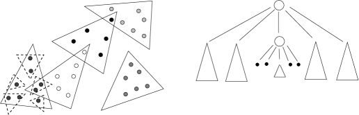
Figure 14: Illustrating a simplicial partition and the corresponding partition tree. The dotted triangles form the partition computed recursively for the class corresponding to the middle child of the root; the resulting five “subclasses” are stored in five subtrees below the middle child.

For each query simplex $\triangle$, the goal is to compute the number of points in $P\cap\triangle$. We start from the root of $T$. For each internal node $v$, we check its simplicial partition $\Pi_{v}$ one by one, and handle directly those contained in $\triangle$ or disjoint from $\triangle$; we proceed with the corresponding child nodes for the other simplices. Each of the latter ones must be intersected by at least one of the lines bounding $\triangle$. If $v$ is a leaf node, for each point $p$ in $P_{v}$, we determine directly whether $p\in\triangle$. Each query takes $O(n^{1/2}(\log n)^{O(1)})$ time [16].

For our purpose, we augment the partition tree $T$ in the following way. For each node $v$, we compute and maintain the Voronoi diagram of $P_{v}$, denoted by $\mbox{$V\!D$}(P_{v})$. Since at each level of $T$ the point subsets $P_{v}$’s are pairwise disjoint, comparing with the original tree, our augmented tree has $O(n)$ additional space at each level. Since $T$ has $O(\log\log n)$ levels, the total space of our augmented tree is $O(n\log\log n)$. For the running time, we claim that the total time for building the augmented tree is still $O(n\log n)$ although we have to build Voronoi diagrams for the nodes. Indeed, let $T(n)$ denote the time for building the Voronoi diagrams in the entire algorithm. We have $T(n)=\sqrt{n}\cdot T(\sqrt{n})+O(n\log n)$, and thus, $T(n)=O(n\log n)$ by solving the above recurrence.

Consider any query triangle $\triangle$ and any point $q$. We start from the root of $T$. For each internal node $v$, we check its simplicial partition $\Pi_{v}$, i.e., check the children of $v$ one by one. Consider any child $u$ of $v$. If $\triangle_{u}$ is disjoint from $\triangle$, we ignore it. If $\triangle_{u}$ is contained in $\triangle$, then we compute in $O(\log n)$ time the closest point of $P\cap\triangle_{u}$ to $q$ (and its distance to $q$) by using the Voronoi diagram $\mbox{$V\!D$}(P_{u})$ stored at the node $u$. Otherwise, we proceed with the node $u$ recursively. If $v$ is a leaf node, for each point $p$ in $P_{v}$, we compute directly the distance $d(q,p)$ if $p\in\triangle$. Finally, $f_{\triangle}(q)$ is the closest point to $q$ among all points whose distances to $q$ have been computed above.

Comparing with the original simplex range query on $\triangle$, we have $O(\log n)$ additional time on each node $u$ if $\triangle_{u}$ is contained in $\triangle$, and clearly the number of such nodes is bounded by $O(n^{1/2}(\log n)^{O(1)})$. Hence, the total query time for finding $f_{\triangle}(q)$ is $O(n^{1/2}(\log n)^{O(1)}\cdot\log n)$, which is $O(n^{1/2}(\log n)^{O(1)})$. The lemma thus follows. $\Box$

Similar augmentation may also be made on the $O(n)$-size simplex data structure in [17] and the recent randomized result in [4]. If more space are allowed, by using duality and cutting trees [6], we can obtain the following result.

Lemma 9

After $O(n^{2+\epsilon})$ time and space preprocessing on $P$, we can compute the point $f_{\triangle}(q)$ in $O(\log n)$ time for any triangle $\triangle$ and any point $q$ in the plane.

Proof: By using duality and cutting trees, an $O(n^{2+\epsilon})$-size data structure can be built in $O(n^{2+\epsilon})$ time for any $\epsilon>0$ such that each simplex range (counting) query can be answered in $O(\log^{3}n)$ time [6]. We can augment the data structure in a similar way as in Lemma 8. We only sketch it below.

The data structure in [6] has three levels. In the third level, each tree node maintains the cardinality of the corresponding canonical subset of points. For our purpose, we explicitly maintain the Voronoi diagram for each canonical subset in the third level. Hence, our augmented data structure has four levels. The preprocessing time and the space are the same as before. The query algorithm is similar as before and the difference is that when a canonical subset of points are all in the query triangle $\triangle$, instead of counting the cardinality of the canonical subset, we determine the closest point to $q$ in the canonical subset by using the Voronoi diagram of the canonical subset. Hence, the total time of our query algorithm is $O(\log^{4}n)$ time.

To reduce the query time, a commonly known approach is to use cutting trees with nodes having degrees $n^{\delta}$ for a certain small constant $\delta>0$. Therefore, the heights of the trees are constant rather than logarithmic, and consequently, the total query time becomes $O(\log n)$. Note that we can use a point location data structure [7, 9] to determine in logarithmic time the child in which we continue the search, but this does not affect the preprocessing time and space asymptotically. The lemma thus follows. $\Box$

Lemmas 7, 8, and 9 together lead to the following theorem.

Theorem 3

Given a set $P$ of $n$ points in the plane, after $O(n\log n\log\log n)$ time and $O(n\log\log n)$ space preprocessing, we can answer each $L_{1}$ ANN-Max query in $O(m\sqrt{n}\log^{O(1)}n)$ time for any set $Q$ of $m$ query points; alternatively, after $O(n^{2+\epsilon})$ time and space preprocessing for any $\epsilon>0$, we can answer each $L_{2}$ ANN-Max query in $O(m\log n)$ time.

References

- [1] P.K. Agarwal, A. Efrat, S. Sankararaman, and W. Zhang. Nearest-neighbor searching under uncertainty. In Proc. of the 31st Symposium on Principles of Database Systems, pages 225–236, 2012.
- [2] S. Arya, D.M. Mount, N.S. Netanyahu, R. Silverman, and A.Y. Wu. An optimal algorithm for approximate nearest neighbor searching fixed dimensions. Journal of the ACM, 45:891–923, 1998.
- [3] F. Aurenhammer and R. Klein. Voronoi Diagram, in Handbook of Computational Geometry, J.-R Sack and J. Urrutia (eds.), chapter 8, pages 201–290. Elsevier, Amsterdam, the Netherlands, 2000.
- [4] T.M. Chan. Optimal partition trees. Discrete and Computational Geometry, 47:661–690, 2012.
- [5] B. Chazelle. An algorithm for segment-dragging and its implementation. Algorithmica, 3(1–4):205–221, 1988.
- [6] M. de Berg, O. Cheong, M. van Kreveld, and M. Overmars. Computational Geometry — Algorithms and Applications. Springer-Verlag, Berlin, 3rd edition, 2008.
- [7] H. Edelsbrunner, L. Guibas, and J. Stolfi. Optimal point location in a monotone subdivision. SIAM Journal on Computing, 15(2):317–340, 1986.
- [8] A. Guttman. R-trees: a dynamic index structure for spatial searching. In Proc. of the ACM SIGMOD International Conference on Management of Data, pages 47–57, 1984.
- [9] D. Kirkpatrick. Optimal search in planar subdivisions. SIAM Journal on Computing, 12(1):28–35, 1983.
- [10] D.T. Lee. On -nearest neighbor voronoi diagrams in the plane. IEEE Transactions on Computers, 31(6):478–487, 1982.
- [11] F. Li, B. Yao, and P. Kumar. Group enclosing queries. IEEE Transactions on Knowledge and Data Engineering, 23:1526–1540, 2011.
- [12] H. Li, H. Lu, B. Huang, and Z. Huang. Two ellipse-based pruning methods for group nearest neighbor queries. In Proc. of the 13th Annual ACM International Workshop on Geographic Information Systems, pages 192–199, 2005.
- [13] Y. Li, F. Li, K. Yi, B. Yao, and M. Wang. Flexible aggregate similarity search. In Proc. of the ACM SIGMOD International Conference on Management of Data, pages 1009–1020, 2011.
- [14] X. Lian and L. Chen. Probabilistic group nearest neighbor queries in uncertain databases. IEEE Transactions on Knowledge and Data Engineering, 20:809–824, 2008.
- [15] Y. Luo, H. Chen, K. Furuse, and N. Ohbo. Efficient methods in finding aggregate nearest neighbor by projection-based filtering. In Proc. of the 12nd International Conference on Computational Science and its Applications, pages 821–833, 2007.
- [16] J. Matoušek. Efficient partition trees. Discrete and Computational Geometry, 8(3):315–334, 1992.
- [17] J. Matoušek. Range searching with efficient hierarchical cuttings. Discrete and Computational Geometry, 10(1):157–182, 1993.
- [18] J.S.B. Mitchell. shortest paths among polygonal obstacles in the plane. Algorithmica, 8(1):55–88, 1992.
- [19] D. Papadias, Q. Shen, Y. Tao, and K. Mouratidis. Group nearest neighbor queries. In Proc. of the 20th International Conference on Data Engineering, pages 301–312, 2004.
- [20] D. Papadias, Y. Tao, K. Mouratidis, and C.K. Hui. Aggregate nearest neighbor queries in spatial databases. ACM Transactions on Database Systems, 30:529–576, 2005.
- [21] M. Sharifzadeh and C. Shahabi. VoR-Tree: R-trees with Voronoi diagrams for efficient processing of spatial nearest neighbor queries. In Proc. of the VLDB Endowment, pages 1231–1242, 2010.
- [22] H. Wang and W. Zhang. The top- nearest neighbor searching with uncertain queries. arXiv:1211.5084, 2013.
- [23] M.L. Yiu, N. Mamoulis, and D. Papadias. Aggregate nearest neighbor queries in road networks. IEEE Transactions on Knowledge and Data Engineering, 17:820–833, 2005.