Nonlocality in Homogeneous Superfluid Turbulence

Abstract

Simulating superfluid turbulence using the localized induction approximation allows neighboring parallel vortices to proliferate. In many circumstances a turbulent tangle becomes unsustainable, degenerating into a series of parallel, non-interacting vortex lines. Calculating with the fully nonlocal Biot-Savart law prevents this difficulty but also increases computation time. Here we use a truncated Biot-Savart integral to investigate the effects of nonlocality on homogeneous turbulence. We find that including the nonlocal interaction up to roughly the spacing between nearest-neighbor vortex segments prevents the parallel alignment from developing, yielding an accurate model of homogeneous superfluid turbulence with less computation time.

Superfulid helium can be described by a two-fluid model as comprised of a normal fluid part with velocity $v_{n}$ and a superfluid part with velocity $v_{s}$. At small velocities, the superfluid exhibits remarkable properties such as the ability to flow without dissipation. But above some critical velocity, turbulence sets in and new interactions must be considered. Schwarz Schwarz (1982) provided a major computational breakthrough in understanding superfluid turbulence as a tangle of vortex filaments, an idea first suggested by Feynman Feynman (1955) and investigated by Vinen Vinen (1957). Each vortex filament is an effectively one-dimensional curve around which superfluid flows. Since the superfluid is incompressible, $\nabla\cdot\vec{v}_{s}=0$, the flow field due to these vortices is determined by the Biot-Savart law. Kelvin’s theorem indicates that vortices move at approximately the local superfluid velocity, meaning that the motion of each segment of the vortex is determined by the positions of all vortices in the tangle. An additional interaction term between the superfluid vortex and the normal fluid gives us the vortex equation of motion:

$$\dot{\vec{s}}(\xi,t)= \vec{v}_{s}+\dot{\vec{s}}_{\mathrm{Biot}}+\alpha\hat{s}^{\,\prime}\times\left(\vec{v}_{ns}-\dot{\vec{s}}_{\mathrm{Biot}}\right)$$

$$-\alpha^{\prime}\hat{s}^{\,\prime}\times\left[\hat{s}^{\,\prime}\times\left(\vec{v}_{ns}-\dot{\vec{s}}_{\mathrm{Biot}}\right)\right],$$ (1)

$$\dot{\vec{s}}_{\mathrm{Biot}}= \frac{\kappa}{4\pi}\int\frac{(\vec{s}_{o}-\vec{s})\times\mathrm{d}\vec{\xi}_{o}}{|\vec{s}_{o}-\vec{s}|^{3}}.$$

Here, $\vec{s}(\xi,t)$ is the position along the vortex, parametrized by the arclength, $\xi$. The circulation $\kappa$ is a fundamental constant for the superfluid vortex and the integral runs over all vortices within the tangle. The vector $\hat{s}^{\,\prime}$ is the unit vector tangent to the vortex filament, along which $\mathrm{d}\vec{\xi}_{o}$ also points. $\alpha$ and $\alpha^{\prime}$ are temperature-dependent parameters characterizing the interaction between the normal fluid and the vortex core, and the quantity $\vec{v}_{ns}$ is equal to $\vec{v}_{n}-\vec{v}_{s}$.

The Biot-Savart integral diverges as the source point $\vec{s}_{o}$ approaches the field point $\vec{s}$, so the integral is split into a local part and nonlocal part (Arms and Hama, 1965; Schwarz, 1985). The local part extends from the radius of the filament core, $a_{0}$, to some arclength, $l_{\pm}$, away from the point of interest. The remainder of the vortex system is included in the nonlocal part of the integral,

$$\dot{\vec{s}}_{\mathrm{Biot}}(\xi,t)= \frac{\kappa}{4\pi}\hat{s}^{\,\prime}\times\vec{s}^{\,\prime\prime}\ln\left(\frac{2(l_{+}l_{-})^{1/2}}{e^{1/4}a_{0}}\right),$$

$$+\frac{\kappa}{4\pi}\int^{\prime}\frac{(\vec{s}_{o}-\vec{s})\times\mathrm{d}\vec{\xi}_{o}}{|\vec{s}_{o}-\vec{s}|^{3}}.$$

Since the local term dominates, the nonlocal part has often been ignored. This is called the localized induction approximation (LIA) or the local approximation. When this is done, there is no objective best cutoff for $l_{\pm}$ in the local term so the average radius of curvature, $\bar{R}$, is used and the coefficient in front of the local term is referred to as $\beta$, sometimes with a constant $c$ of order unity included:

$$\beta=\frac{\kappa}{4\pi}\ln\left(\frac{\bar{R}}{ca_{0}}\right).$$

Vortex behavior is strongly influenced by vortex reconnections: vortices can approach and touch at a point, exchange heads and tails, then withdraw. Schwarz Schwarz (1985) investigated these events, arguing that the process could be modeled by an instantaneous swap once two vortex segments approach within some cutoff distance. When the LIA is employed, vortex reconnections are the only nonlocal interaction involved in the simulation.

I Motivation: Open-Orbit Vortices

Schwarz’s early simulations Schwarz (1985) apparently produced sustained homogeneous turbulence. However, Buttke Buttke (1987) could only reproduce the results by using deliberately inadequate spatial resolution. Buttke subsequently argued Buttke (1988) that since LIA does not allow vortex stretching, it cannot describe superfluid turbulence. However, Schwarz Schwarz (1987) attributed the difference in computational results to an artifact of the simulation geometry. With periodic boundary conditions, a vortex line can cross the entire volume and close on itself. Energy loss will increase the radius of curvature of such an “open-orbit” vortex until the vortex is entirely straight and interacts with the applied velocity field only through an overall translation. No further energy is transfered between the applied field and the vortex. The LIA contribution to the velocity of a straight open-orbit vortex also vanishes, so only a reconnection can disrupt its stability. In extreme cases the entire system can degenerate to an open-orbit state, where all the vortices align and straighten into a clearly non-homogeneous state that can persist indefinitely. Figures 1c and 1f show such an open-orbit state. To prevent the open-orbit state from developing, Schwarz Schwarz (1988) inserted an occasional mixing step, in which half the vortices, selected at random, were rotated by 90^∘ about the direction of the applied flow. Buttke’s simulations, lacking this artificial mixing procedure, gave quite different results.

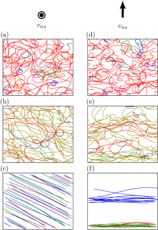
Figure 1: Projections of vortex tangles from the present work, with applied velocity perpendicular to (a-c) or within (d-f) the viewing plane. All computations use $v_{ns}=11$ cm/s, in a periodic cube with side length $50\mu$m. The first row shows full Biot-Savart law calculation at time 0.142 s. The second and third rows show the LIA calculation at times 0.9 s and 0.142 s, respectively. In frames (b) and (e) the tangle has begun to exhibit anisotropy; in frames (c) and (f) the system has reached an open-orbit state, with the vortices almost entirely straight and parallel.

Various other methods of avoiding the open-orbit state have been used. Schwarz attributed the state to the periodic boundary conditions since it did not occur when he used the much more computationally expensive real-wall boundaries; however, the resulting tangles are not statistically identical to those generated with periodic boundary conditions and a mixing step(Schwarz, 1988). AartsAarts (1993) does not include mixing, but instead focuses on the time domain after the vortex line length equilibrates but before the system degenerates into the open-orbit state. Adachi et al. Adachi et al. (2010) find that retaining the nonlocal terms instead of using the LIA eliminates the need for any special accommodations to fix or avoid the open-orbit state, suggesting that the LIA rather than the boundary conditions may be at the root of the problem. Yet, as NemirovskiiNemirovskii (2013) notes, it is unclear why the nonlocal term should be so effective, since nothing in the Biot-Savart integral prevents the types of reconnections that produce open-orbit vortices.

Kondaurova et al.Kondaurova et al. (2008) suggest the vortex reconnection condition as another possible source of trouble. Instead of basing reconnection solely on the locations of neighboring vortices, they consider the velocities of nearby vortex segments and carry out a reconnection only if the segments would cross through each other during the time step. In a study comparing several reconnection algorithms, BaggaleyBaggaley (2012) finds that the reconnection details have little statistical effect on the vortex tangle in a nonlocal (Biot-Savart) calculation. However, results from LIA calculations do depend heavily on when and how reconnections are carried out. Once again this hints at a sickness in the LIA.

Here we propose yet another scheme for calculating the vortex motion between reconnections. We include only those portions of the Biot-Savart integral where $|\vec{s}_{o}-\vec{s}|$ is smaller than a nonlocal interaction distance $d_{NL}$, and we vary $d_{NL}$ from 0 to interactions that span the computational volume. Our results confirm that the LIA does not suffice for modeling superfluid turbulence, but we find that only a small region of nonlocal interaction is needed to reach accurate results. Our calculations also shed light on some of the behaviors observed in previous computational work.

II Results from the Full Biot-Savart Integral and the LIA

We first present data using the full Biot-Savart integral and the LIA to show that our code is in good agreement with previous simulations and experiment. We run simulations at temperature $T\approx 1.6$ K, which corresponds to $\alpha=0.1$. We ignore $\alpha^{\prime}$ since it is an order of magnitude smaller, and we use $v_{n}$ as our driving velocity ($v_{s}=0$) throughout this work to eliminate uniform vortex translation. Except as otherwise noted, we use a periodic cube with side length $D=50\mu$m. Our equation of motion is integrated using a Runge-Kutta-Fehlberg method (RKF54) with an adaptive time step. Our point spacing is also adaptive, depending on the local radius of curvature within the range $R/12\leq l\leq R/5$. As the vortex grows and a particular point spacing exceeds the upper limit, we add a new point along a circular arc determined by the points that neighbor this overlarge spacing, as described by SchwarzSchwarz (1985). In practice the time step is usually about $2\times 10^{-6}$ s, and the spacing between points is about $8\times 10^{-5}$ cm. We carry out a reconnection when vortices approach within $2R_{min}/\ln(R_{min}/a_{0})$, where $R_{min}$ is the smaller radius of curvature at the points in question. The separation must also be below an absolute cutoff, generally 10 $\mu$m. For our homogeneous vortex tangles, the absolute level typically exceeds the curvature-based cutoff by more than an order of magnitude and plays little role in the dynamics. As we discuss below, the absolute cutoff becomes relevant in the untangled open-orbit state produced with the LIA. We perform the reconnections themselves so as not to increase the total vortex line length, by adjusting the position along the vortex of the points involved in the reconnectionDix (2012).

We shall compare the LIA and full Biot-Savart calculations in multiple ways, including through visual inspection (as in Figure 1), using the line length density given by

$$L=\frac{1}{V}\int\mathrm{d}\xi,$$ (2)

where $V$ is the system volume, and with measures of the anisotropy given by (Schwarz, 1988):

$$I_{\parallel}=\frac{1}{VL}\int\left[1-\left(\hat{s}^{\,\prime}\cdot\hat{r}_{\parallel}\right)^{2}\right]d\xi,$$ (3)

$$I_{\perp}=\frac{1}{VL}\int\left[1-\left(\hat{s}^{\,\prime}\cdot\hat{r}_{\perp}\right)^{2}\right]d\xi,$$ (4)

$$I_{\ell}\hat{r}_{\parallel}=\frac{1}{VL^{3/2}}\int\hat{s}^{\,\prime}\times\vec{s}^{\,\prime\prime}d\xi.$$ (5)

Here $\hat{r}_{\parallel}$ and $\hat{r}_{\perp}$ are unit vectors parallel and perpendicular to the $\vec{v}_{ns}$ direction. As long as both directions perpendicular to the flow velocity are equivalent, the following relation is true regardless of tangle geometry: $I_{\parallel}/2+I_{\perp}=1$. Note also that if a vortex tangle is completely isotropic, $I_{\parallel}=I_{\perp}=2/3$ and $I_{\ell}=0$. If vortices lie entirely within planes normal to $\vec{v}_{ns}$, $I_{\parallel}=1$, $I_{\perp}=1/2$, and $I_{\ell}$ will depend on the structure of the vortices.

Figure 2 compares $L(t)$ and $I_{\parallel}(t)$ for calculations with the LIA and full Biot-Savart law. The data agree well with those of Adachi et al.Adachi et al. (2010), with small differences arising from different system sizes and driving velocities.

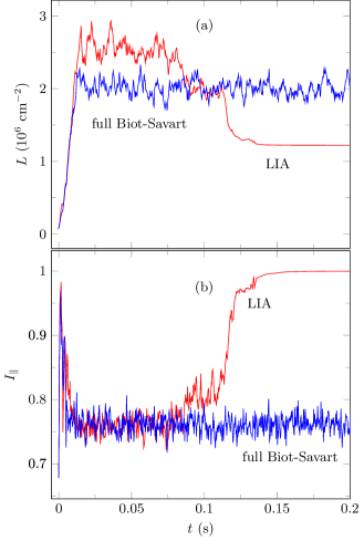
Figure 2: Results from LIA and full Biot-Savart calculations for (a) $L(t)$ and (b) $I_{\parallel}(t)$, with $v_{ns}=11$ cm/s.

Clearly the LIA results deviate significantly from those of the fully nonlocal calculation. The presence of nonlocal interactions reduces the vortex line length density. As Adachi et al.Adachi et al. (2010) explain, the nonlocal interaction is strongest immediately before and after a reconnection, when vortices are closest. The nonlocal term tends to repel two parallel vortex segments and attract antiparallel segments. Consequently, fewer parallel reconnections occur when the nonlocal interaction is included. Furthermore, reconnections between antiparallel segments produce highly curved regions that retreat away from the reconnection site quickly. By contrast, reconnections of parallel vortices result in more gently curved segments that do not retreat quickly. The net result of these effects is that the nonlocal interaction increases the average intervortex separation and correspondingly decreases the line length density.

Figure 1 shows several snapshots from these simulations. The first row is a homogeneous tangle from the full Biot-Savart calculation. The LIA tangle appears similar for $0.02<t<0.08$ s, a nearly steady-state regime. Aarts Aarts (1993) uses this regime to evaluate properties of the vortex tangle. At later times, the system collapses into the open-orbit state, with vortices aligning perpendicular to the driving velocity. The second and third rows of Figure 1 illustrate configurations during the collapse and after its completion. How quickly the open-orbit state forms depends strongly on the exact parameters used for a simulation. For example, it appears more quickly at high driving velocities, where the growth of line length in the plane perpendicular to the applied velocity helps to nucleate the open-orbit state. In some cases the intermediate, partially collapsed state can continue for significant times, possibly indefinitely. The density of the open-orbit state is an artificial value, determined by the absolute cutoff distance used for reconnections. While this value plays almost no role for a highly tangled state, it becomes the de facto reconnection distance as vortices form open orbits and straighten. In the final state, neighboring vortices are spaced far enough apart to avoid further reconnections.

We demonstrate homogeneity of the full Biot-Savart calculation directly by finding the average line length density in different constituent volumes within the system (Equation 2). Figure 3 shows a sample evolution of $L(t)$. We use the eight $\mathbb{R}^{3}$ octants as the volumes to calculate each curve.

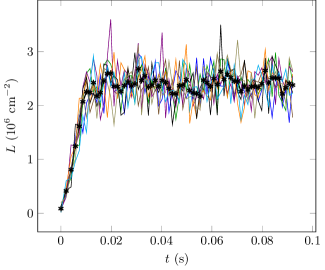
Figure 3: Evolution of the vortex line length density, $L(t)$, within each octant of the periodic cube. The curve marked by black asterisks gives the line length per total system volume, $D^{3}$. Each other curve gives $L(t)$ for one of the eight $\mathbb{R}^{3}$ octants. The applied velocity is $v_{n}=12$ cm/s.

Even after steady-state turbulence has set in, we expect some variation in $L(t)$ among the octants, but the average equilibrated values should be the same. Figure 4 shows these average equilibrated $L$ values for each octant, for a range of driving velocities. Time averages were done over the equilibrated time domain. We use the bracket notation $\langle X\rangle$ to denote the time average, as opposed to averages over the length of the vortex at a fixed time for which we use the notation $\bar{X}$. From Figure 4, it is clear that on this scale our system is homogeneous at every velocity.

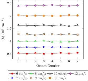
Figure 4: Average equilibrated line length density, $\langle L\rangle$, within each octant of the periodic cube, at multiple velocities.

Scaling arguments provide an additional test of homogeneous turbulence. Simple dimensional analysis shows that the line length density in homogeneous turbulence should depend on the driving velocity as(Schwarz, 1988)

$$\langle L\rangle=c_{L}^{2}(v_{ns}/\beta)^{2},$$ (6)

where $c_{L}$ is temperature-dependent. As noted previously, $\beta$ depends logarithmically on the average local radius of curvature, which decreases with increasing velocity. To keep $c_{L}$ independent of velocity, we do not combine $\beta$ with $c_{L}$. As shown in Figure 5, our simulations closely follow this scaling law. The best-fit value of $c_{L}$ is 0.106.

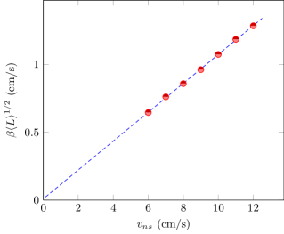
Figure 5: Average equilibrated line length density, $\langle L\rangle$, for the total system volume, at multiple velocities. The linear fit to our data yields a slope of $c_{L}=0.106$.

Another scaling check of our simulations comes through the mutual friction force density due to interactions between the normal fluid and superfluid components. This force results in the interaction term of the vortex equation of motion ($\vec{v}_{fric}$),

$$\vec{F}_{sn}=-\frac{\rho_{s}\kappa}{V}\hat{s}^{\,\prime}\times\vec{v}_{fric},$$ (7)

where $V$ is the system volume. When averaged along the entire vortex, only $\bar{F}_{sn}$ parallel to the driving velocity is non-negligible. Schwarz Schwarz (1988) also developed a scaling relation for the equilibrated force, $\langle\bar{F}_{sn}\rangle\propto v_{ns}^{3}/\beta^{2}$. We construct a new quantity:

$$\bar{\Gamma}:=\frac{\bar{F}_{sn}}{\rho_{s}\kappa\alpha v_{ns}},$$ (8)

which we can fit in the form $\beta\langle\bar{\Gamma}\rangle^{1/2}=c_{F}v_{ns}+y_{0}$, as shown in Figure 6. The linear fit shows a slope of $c_{F}=0.088$ with no $y$-intercept, as theory predicts.

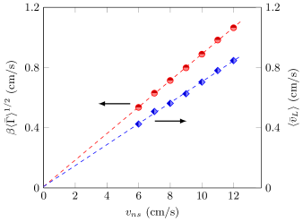
Figure 6: Left axis (red circles): The quantity $\langle\bar{\Gamma}\rangle$ taken from the mutual friction force density, $\bar{F}_{sn}$ along $\hat{v}_{ns}$. The linear fit of this data yields a slope of $c_{F}=0.088$. Right axis (blue diamonds): The average vortex velocity, $\bar{v}_{L}$. The linear fit of this data yields a slope of $c_{v}=0.070$.

Yet another quantity used to describe homogeneous superfluid turbulence is the average vortex velocity relative to the applied superfluid velocity $\vec{v}_{s}$:

$$\bar{v}_{L}=\left[\frac{1}{VL}\int\dot{s}\mathrm{d}\xi\right]-\vec{v}_{s}.$$ (9)

As for $\bar{F}_{sn}$, only the component of $\bar{v}_{L}$ in the direction of the driving velocity is non-negligible. This time the quantity in question requires no scaling with $\beta$: $\bar{v}_{L}/v_{ns}=b(T)$, where $b(T)$ is a temperature-dependent parameter (Tough, 1982; Schwarz, 1988). Our data for $\bar{v}_{L}$ are shown in Figure 6.

The anisotropy parameters from Equations 3 through 5 are also consistent with previous simulations: $\langle I_{\parallel}\rangle=0.761$, $\langle I_{\perp}\rangle=0.620$, $\langle I_{\ell}\rangle=0.646$. These values show no significant trend over our range of $v_{ns}$. Schwarz Schwarz (1988) points out that under the LIA, the average mutual friction force density $\bar{F}_{sn}$ along $\hat{v}_{ns}$ can be written as:

$$\bar{F}_{sn}=\rho_{s}\kappa\alpha(c_{L}^{2}I_{\parallel}-c_{L}^{3}I_{\ell})v_{ns}^{3}/\beta^{2}.$$ (10)

As we have defined it, then:

$$\bar{\Gamma}=(c_{L}^{2}I_{\parallel}-c_{L}^{3}I_{\ell})\left(\frac{v_{ns}}{\beta}\right)^{2}.$$

We can see that the quantity $c_{F}$, obtained earlier from the mutual friction force density data, is equal to $(c_{L}^{2}I_{\parallel}-c_{L}^{3}I_{\ell})^{1/2}$.

Equation 10 is only approximate when nonlocal contributions are included through the Biot-Savart law; hence we expect our calculations to produce slightly different values from those of Schwarz Schwarz (1988) and Aarts Aarts (1993), who used the LIA. Additionally, Schwarz Schwarz (1988) states that, when neglecting $\alpha^{\prime}$, the slope parameter we call $c_{v}$ is equal to $c_{L}I_{\ell}$, again assuming the LIA. With these relations, we compare characteristics of homogeneous turbulence in our own simulations and in previous works, in Table 1. We use $c_{v}$ or $c_{L}I_{\ell}$, depending on which can be derived from the data shown in earlier works. Similarly, we use $c_{F}$ or $(c_{L}^{2}I_{\parallel}-c_{L}^{3}I_{l})^{1/2}$. Schwarz Schwarz (1988) does show that his theoretical calculations of $I_{\perp}/I_{\parallel}$, $(c_{L}^{2}I_{\parallel}-c_{L}^{3}I_{\ell})^{1/2}$, and $c_{L}I_{\ell}$ match experiment.

Source (T=1.6 K)	$c_{L}$	$I_{\perp}/I_{\parallel}$	$c_{F}$	$(c_{L}^{2}I_{\parallel}-c_{L}^{3}I_{\ell})^{1/2}$	$c_{v}$	$c_{L}I_{\ell}$
Present Work	0.106	0.815	0.088	0.088	0.070	0.069
AartsAarts (1993)	0.11	-	0.095†	-	0.045†	-
SchwarzSchwarz (1988)	0.137	0.775‡	-	0.116†	-	0.063†

Table 1: Comparison of quantities characterizing homogeneous turbulence. $\dagger$: value calculated from other reported quantities; $\ddagger$: value estimated from published figure.

Both Adachi et al.Adachi et al. (2010) and Kondaurova et al.Kondaurova et al. (2008) report $\gamma=c_{L}/\langle\beta\rangle$ rather than $c_{L}$ itself. Doing so requires one to insert an ad hoc $y$-intercept to maintain a decent linear fit. When we do this, we get a value of $\gamma=137.3$ s/cm², where Adachi et al.Adachi et al. (2010) report a value of $\gamma=109.6$ s/cm². The experimental value is $\gamma=93$ s/cm²  (Childers and Tough, 1976; Tough, 1982). We can extract the value for $I_{\perp}/I_{\parallel}\approx 0.8$ from Adachi et al.Adachi et al. (2010), which also matches our quantity from Table 1 of $0.815$. Kondaurova et al.Kondaurova et al. (2008) find $\gamma=280$ s/cm², which is extremely high. In more recent work by the same lead authorKondaurova et al. (2014), $\gamma$ ranges from 105.8 to 120.2 s/cm² at 1.6 K, depending on the reconnection criterion used. The difference may be from the larger sample volume and much lower applied fluid velocities used for the later calculations.

A final test is the rate of vortex reconnections, an important process in carrying energy down to smaller length scales. Previous simulations and analysis show that the rate of vortex reconnections is related to the line length density by $\dot{n}=C\kappa\langle L\rangle^{5/2}$, where $\dot{n}$ is the reconnection rate per unit volume and $C$ is a dimensionless constant with a value of approximately 0.1-0.5  (Tsubota et al., 2000; Barenghi and Samuels, 2004; Nemirovskii, 2006; Kondaurova et al., 2014). Once again the earlier Kondaurova et al.Kondaurova et al. (2008) results are outliers, with an overlarge prefactor of $C=2.47$. Figure 7 gives our data on the vortex reconnection rate for a series of trials. We find an exponent of 2.47 and $C=0.42$, within the normal range.

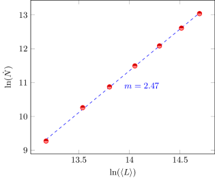
Figure 7: A plot of $\ln(\dot{N})$ versus $\ln(\langle L\rangle)$, finding the exponent of $\dot{N}=\mathrm{d}N/\mathrm{d}t\propto\langle L\rangle^{m}$, $m=2.47$.

Our full Biot-Savart calculation matches previous calculations of homogeneous superfluid turbulence through multiple comparisons.

III Nonlocal Distance, $d_{NL}$

In this section, we investigate further the finding by Adachi et al.Adachi et al. (2010) that the LIA approximation is inadequate for producing homogeneous turbulence. We saw in Figure 2 that despite the fact that $L$ retains an approximate $\langle L\rangle\propto v^{2}$ relationship (Schwarz, 1988; Aarts, 1993), and even in a time domain before the open-orbit vortex state dominates, $L$ still deviates significantly between the LIA and full Biot-Savart calculations. The two methods do produce equally isotropic systems, however. For certain limited objectives, such as Schwarz’s(Schwarz, 1982, 1988) efforts to identify the attributes necessary for a given behavior, the LIA may be an acceptable approximation.

Here we investigate whether some degree of the computation-saving power found in the LIA could be retained by truncating the nonlocal interaction at a distance which we denote by $d_{NL}$. For each point on the vortex, we only include contributions to the Biot-Savart integral, Equation 1, from vortex segments that are within a distance $d_{NL}$ of the evaluation point. Our results for $\langle L\rangle^{1/2}(v_{ns})$ are displayed in Figure 8, for a range of $d_{NL}$ values.

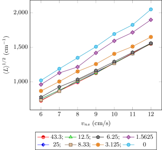
Figure 8: Effects of nonlocal distance, $d_{NL}$, on the equilibrated line length density, $\langle L\rangle$. Each curve is a series of trials at the $d_{NL}$, listed in the legend. The side length for the sample region is $D=50\mu$m, and the largest $d_{NL}$ allows interactions throughout the volume. Averages at each $v_{ns}$ used the initial equilibrated range, similar to AartsAarts (1993).

For a sample volume with side $D=50\mu$m, Biot-Savart interactions among all pairs of vortices occur at $d_{NL}=\sqrt{3}D/2=43.3\mu$m. As $d_{NL}$ decreases from this maximum value, the data at first remain remarkably similar to those using the maximum $d_{NL}$. Eventually the data begin to deviate, with the line-length density increasing above its value from the full calculation. The onset of this divergence is even more apparent in Figure 9, which plots the root-mean-square (RMS) deviation of $\langle L\rangle$ from the full Biot-Savart value:

$$\delta_{rms}(\langle L\rangle)=\left\langle\left(\frac{\langle L\rangle-\langle L_{BS}\rangle}{\langle L_{BS}\rangle}\right)^{2}\right\rangle_{v_{ns}}^{1/2}.$$ (11)

Here $\langle\ldots\rangle_{v_{ns}}$ represents the average over trials with different $v_{ns}$ values but the same $d_{NL}$. The quantity in Equation 11 acts as a measure of the error in our calculation due to the truncated nonlocal interaction. Figure 9 shows how this quantity varies with $d_{NL}$.

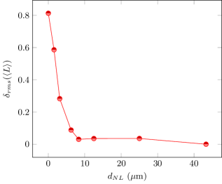
Figure 9: RMS fractional deviation of $\langle L\rangle$ from the full Biot-Savart calculation for several nonlocal distances. Box side is $50\mu$m. The trials contributing to each point are from Figure 8, and use the initial equilibrated time domain for calculating the average of $L(t)$.

Truncated nonlocal distances of at least $8.33\mu$m show good agreement ($\lesssim 5\%$) with the full Biot-Savart calculation, but a clear departure arises by $6.25\mu$m.

These time averages all use the initial equilibrated time domain before the characteristic drop in $L(t)$, seen in Figure 2, i.e. before the degeneration into the open-orbit state occurs at the lower $d_{NL}$ values. However, the subjectivity in selecting the time domain over which to average $L(t)$ could potentially affect the $d_{NL}$ needed for agreement with the full Biot-Savart calculation. An alternative approach, for conditions that result in the open-orbit state, is to calculate the standard deviation of $L(t)$ over the entire time domain after the initial equilibration. The drop in $L(t)$ upon entering the open-orbit state sharply increases the standard deviation. Similarly, since from Figure 2, $I_{\parallel}$ only deviates from the full Biot-Savart value outside of the initial equilibrated range, we can also use this quantity and its standard deviation as indicators of an adequate $d_{NL}$. There is still a limited sample of data, since we cannot run trials forever, and we still have to pick out a time when the data start to equilibrate. Figure 10 shows the RMS fractional deviation of $\sigma(L(t))$, $\sigma(I_{\parallel}(t))$, $\langle L\rangle$, and $\langle I_{\parallel}\rangle$ (making the appropriate substitutions into Equation 11) for the trials from Figure 9 using the entire equilibrated time domain.

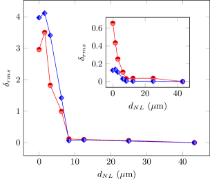
Figure 10: RMS fractional deviation of the standard deviations $\sigma(L(t))$ (red circles) and $\sigma(I_{\parallel}(t))$ (blue diamonds) from the full Biot-Savart calculation plotted versus nonlocal distance. Inset: RMS fractional deviation of the averages $\langle L\rangle$ (red circles) and $\langle I_{\parallel}\rangle$ (blue diamonds) from the full Biot-Savart calculation plotted versus nonlocal distance. Averages use the entire equilibrated time domain. Comparing $\langle L\rangle$ in the inset here to the data in Figure 9 shows the effect of changing the time domain used for the averaging.

From the inset of Figure 10 we see that the critical $d_{NL}$ value is $\lesssim 8.33\mu$m, the same whether we use the entire equilibrated time domain in the averages of $L(t)$ and $I_{\parallel}(t)$ or simply the initial time domain, like in Figure 9. The main part of Figure 10 shows that the standard deviations of $L(t)$ and $I_{\parallel}(t)$ are very good parameters for measuring this critical $d_{NL}$, showing a pronounced increase in error for nonlocal distances below this same critical value. We can use a small fraction of the nonlocal interaction volume and still get a very good approximation of the Biot-Savart integral for homogeneous superfluid turbulence.

While Figures 9 and 10 show averaged results over trials at several values of driving velocity, Figure 11 breaks out the behavior of line length as a function of driving velocity for several nonlocal distances $d_{NL}$.

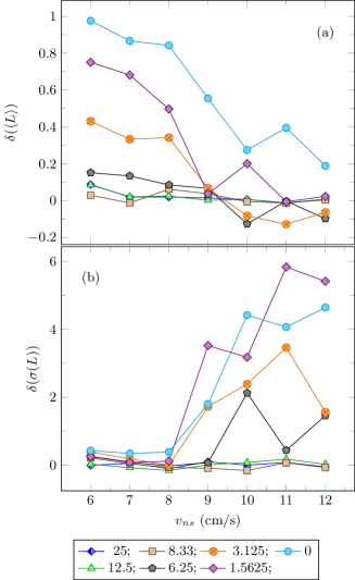
Figure 11: Fractional deviation of (a) $\langle L\rangle$, and (b) $\sigma(L(t))$, from the full Biot-Savart calculation plotted versus driving velocity. Each curve is a different nonlocal distance, $d_{NL}$, indicated by the legend. Averages use the entire equilibrated time domain.

For a fixed $d_{NL}$, deviations of $\langle L\rangle$ from the full nonlocal calculation are more pronounced at the lowest velocities. At high velocity $\langle L\rangle$ is often an average of an initial equilibrated level above that of the full Biot-Savart calculation, and a later level below the Biot-Savart value. The overall $\langle L\rangle$ depends on the amount of time spent in each regime and has little real significance; it may even be coincidentally close to the correct value. For $\sigma(L(t))$ the reverse is true, with deviations larger at higher velocities. The slight enhancement of $\langle L\rangle$ in the initially equilibrated state has little effect on $\sigma(L(t))$, but the collapse to the open-orbit state drastically increases its value. $\langle I_{\parallel}\rangle$ and $\sigma(I_{\parallel}(t))$, not shown in the figure, also deviate more at higher velocities. As shown in Figure 2 (b), $\langle I_{\parallel}\rangle$ matches that of the full Biot-Savart calculations until onset of the open-orbit state, which occurs only for our higher velocities. The abrupt shift in $\langle I_{\parallel}\rangle$ also increases $\sigma(I_{\parallel}(t)$. Because of the different aspects measured by these quantities, calculating several of them is useful for finding any discrepancies from the full Biot-Savart calculations. From a practical perspective, regardless of the underlying cause of any difference, we want to choose an interaction distance such that every driving velocity we use produces turbulent behavior matching the full Biot-Savart law. Our previous averages over all velocities at one $d_{NL}$ pick out deviations at any $v_{ns}$, and larger number of trials contributiong to each curve reduces the scatter so that the critical interaction distance becomes clear.

We next examine how this critical interaction distance varies with system size. We simulated turbulence in three other system sizes, with other parameters held constant. $\langle L\rangle$ data for all three system sizes are shown in Figure 12.

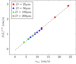
Figure 12: $\beta\langle L\rangle^{1/2}$ data for full Biot-Savart calculations at several system sizes $D$. Averages use the entire equilibrated time domain.

The good agreement in $\langle L\rangle$ for different system sizes is another mark of homogeneity. Since $\langle L\rangle$ is an intensive quantity, with a homogeneous system it must be independent of system size. Figure 13 illustrates the line length in the initial equilibrated region, for the three sizes tested at applied velocity of 9 cm/s. The line length density changes slightly with cell size, but for a given cell size it remains constant for interaction distances at least $12.5\mu$m. For a fixed velocity, the necessary interaction distance does not depend on system size.

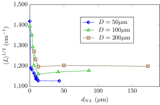
Figure 13: Square root of line length density as function of interaction distance $d_{NL}$, for three box sizes $D$. In each case $\alpha=0.1$ and $v_{ns}=9$ cm/s.

IV Discussion

Similar calculations with other friction coefficients $\alpha$ and applied velocities $v_{ns}$ shed light on why the non-local interaction need only be retained for a portion of the cell volume. Our trials with smaller $\alpha$ are related to lower temperatures, although an attempt to model real behavior of superfluid helium for these values of $\alpha$ would have to include the additional $\alpha^{\prime}$ term that we neglect. The critical interaction distance is as low as $4\mu$m, for the lowest friction and highest velocity. We unfortunately cannot keep $v_{ns}$ entirely fixed while varying $\alpha$. At the velocities of 9-11 cm/s used in much of this work, turbulence is unsustainable for $\alpha=0.01$, when less energy is drawn from the driving velocity field. On the other hand, velocities of 20 cm/s or 50 cm/s, which work for $\alpha=0.01$, would take impractically long with $\alpha=0.1$.

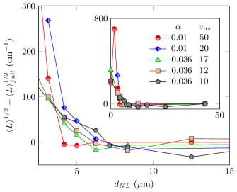
Figure 14: Excess line length as a function of interaction distance, for several combinations of friction parameter $\alpha$ and applied velocity $v_{ns}$. For each curve $\langle L\rangle^{1/2}$ for the largest $d_{NL}$ is subtracted. Main graph: expanded view near critical interaction distance. Inset: entire range. The legend identifies each curve by $\alpha$ and $v_{ns}$, the latter measured in cm/s.

Figure 14 shows results from several trials with lower friction coefficient. The critical interaction distance changes noticeably among the trials, generally decreasing as $v_{ns}$ increases. We suggest that a key issue is the relationship of $d_{NL}$ to the typical intervortex spacing. Clearly the non-local term has minimal effect if the calculation volume includes only a single, relatively straight vortex segment along which the velocity field is being calculated. To significantly alter the LIA simulation, $d_{NL}$ must be larger than either the typical vortex separation or the typical vortex radius of curvature. In the former case, the Biot-Savart calculation would add an interaction between neighboring vortices too distance for an immediate reconnection. In the latter case, the time development of a single contorted filament would change. This is probably most relevant for highly curved vortices, where self-reconnections are especially likely.

The typical vortex separation $\ell$ can be estimated from the line length through $\ell=\langle L\rangle^{-1/2}$. For straight, parallel vortices in a square lattice, this formula gives exactly the nearest-neighbor separation. The calculation is not exact for other lattices, let alone for a tangle of curved vortices, but $\ell$ does give a sense of the intervortex distance.

Table 2 shows the critical interaction distance along with the typical vortex separation and the average radius of curvature. The critical $d_{NL}$ does seem related to $\langle R\rangle$. In fact, the turn-ups for the different curves of Figure 14 are ordered exactly by the $\langle R\rangle$ values. The relationship to $\ell$ is less clear. This is hardly surprising, given that the relation of $\ell$ to the nearest-neighbor vortex spacing is inexact and depends on features like the typical radius of curvature in the tangle. In any case, the necessary $d_{NL}$ apparently has the same order of magnitude as $\ell$.

$\alpha$	$v_{ns}$ (cm/s)	critical $d_{NL}$	$\hskip 14.45377pt\ell$	$\langle R\rangle$
0.01	50	4	5.8	3.7
0.01	20	6	13.1	6.6
0.036	17	6	7.5	4.8
0.036	12	6	10.6	6.3
0.036	10	7	12.5	7.5
0.1	9	9	8.9	6.3

Table 2: Onset of deviation from non-local calculation, compared to the typical intervortex distance and the average radius of curvature. All lengths are given in $\mu$m. The critical $d_{NL}$ is identified as the smallest $d_{NL}$ with results indistinguishable by our measures from the full Biot-Savart calculation. In each case we used 1 $\mu$m steps in $d_{NL}$ near the critical value.

Finding the critical $d_{NL}$ comparable to the typical vortex separation suggests that the key effect of the nonlocal interaction is to draw together nearby vortex segments until they are within the reconnection distance. In the LIA, neighboring vortices are invisible to each other unless they happen to drift close enough to reconnect. If an extra, small attraction from their Biot-Savart interaction results in a reconnection that would not otherwise have occured, it has a significant impact on the subsequent motion. This finding makes sense in light of the open-orbit problem. An occasional open-orbit vortex need not doom a simulation if further reconnections free the vortex from its open-orbit state. Only a collective alignment of open-orbit vortices persists indefinitely. The occasional rotation step that SchwarzSchwarz (1988) used to sustain a vortex tangle operates exactly by ensuring reconnections. Our findings explain why the non-local calculation prevents the simultaneous degeneration of vortices into the open-orbit state. As Nemirovskii notes(Nemirovskii, 2013, p. 152), the addition of non-local contributions cannot prevent the reconnections that lead to open-orbit vortices. Rather, the non-local term enables additional reconnections that disrupt the system from settling into a collective open-orbit configuration.

Beyond the intervortex spacing, the nonlocal contribution is apparently negligible. This is consistent with the rapid fall-off of the Biot-Savart law. In addition, for a random tangle the number of vortex segments a given distance from a calculation point increases as the square of the distance, and the multiple interactions partially cancel, further reducing the total. The unimportance of distant non-local terms has been remarked on previously. A complete Biot-Savart calculation with periodic boundary conditions would require tiling space with the computational volume and adding contributions from each copy of the tangle. Although Ewald summation provides a rapidly-converging technique Toukmaji and Board Jr. (1996), it has not been applied to vortex-filament simulations. However, Kondaurova et al.Kondaurova et al. (2014) find that surrounding the main region with 26 replicas has negligible effect on the results. Our own “full” Biot-Savart calculation uses the main volume, with just a few of the closest image vortices included as well. While it has been standard practice to exclude very distant contributions, we now argue that much of the contribution from within the main volume can also be safely omitted. Yet another effort, in a similar direction, is Baggaley’s recent tree methodBaggaley and Barenghi (2012). Baggaley essentially averages groups of more distance vortex segments before evaluating the Biot-Savart law, and finds good agreement with the full Biot-Savart calculations of Adachi et al.Adachi et al. (2010). This is to be expected since Baggaley’s method has minimal averaging for very close vortex segments. Those are often treated the same as in the Adachi calculation. Averaging over more distant segments has a negligible effect on the statistical properties of the tangle, as does our truncating the Biot-Savart law to omit these segments entirely.

Reducing the interaction distance to such a degree can provide considerable savings in computation time. With interactions omitted beyond $8.33\mu$m in a box of side $50\mu$m, the interaction volume for each vortex segment is about $2\%$ of the entire box: when the system is homogeneous, each segment will have only $1/50$ of the other vortex segments contributing to its nonlocal velocity. Since other calculations must be performed for each point in the tangle, the end result is that simulations with the reduced interaction distance take $1/3$ to $1/10$ of the computation time. The savings could be greater for larger computational volumes or higher driving velocities. A question of practical interest is how small an interaction distance can safely be used. Our results suggest that ensuring interactions from neighboring vortices should be adequate. Furthermore, a possible $d_{NL}$ need not be tested against the full Biot-Savart calculation. It is enough to obtain equivalent results from a few trials with different $d_{NL}$, all of which can be small compared to the entire cell size.

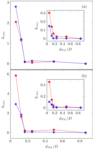
Figure 15: For comparison with Figure 10: Figure (a) has system size $D=25\mu$m, Figure (b) has $D=100\mu$m. RMS fractional deviation from the full Biot-Savart calculation of the standard deviations $\sigma(L(t))$ (red circles) and $\sigma(I_{\parallel}(t))$ (blue diamonds), plotted versus nonlocal distance. Insets: RMS fractional deviation from the full Biot-Savart calculation of $\langle L\rangle$ (red circles) and $\langle I_{\parallel}\rangle$ (blue diamonds), plotted versus nonlocal distance. Time averages use the entire time domain after initial equilibration.

As noted previously, in many cases a single $d_{NL}$ may be desired across a range of velocities. Usable velocities vary with cell size, as shown in Figure 12. When the velocity is too low, tangles are not self-sustaining. When it is too high, the total vortex length and hence the computational time become prohibitive. As a practical matter, the necessary interaction distance then becomes dependent on cell size as well. For the present calculations with $\alpha=0.1$, we find that $d_{NL}=D/6$ is appropriate for several cell sizes. Figure 15 illustrates how deviations from the full non-local calculation begin for two cell sizes, with the velocity ranges of Figure 12.

V Conclusion

Adachi et al.Adachi et al. (2010) show the importance of the nonlocal interaction for homogeneous superfluid turbulence behavior, especially when simulating this system using periodic boundaries. By using a truncated Biot-Savart integral, we have found it possible to regain much of the time saved with the localized induction approximation while still accurately modeling the statistical behavior of the system. We find that the nonlocal interaction is only important up to distances of about the intervortex spacing.

Finally, we address the longstanding question of whether the trouble with obtaining reproducible results on vortex tangles lies with the LIA, the reconnection procedure, or the periodic boundary conditions. Our answer is that the LIA is the main culprit. Its sicknesses cause unusual sensitivity to other details of the simulation, as shown previouslyBaggaley (2012) in the case of reconnection requirements. Worse, its results can deviate quantitatively from those of other techniques, even when no qualitatively obvious problem arises. However, the reason behind the problems with the LIA is primarily its inaccurate treatment of neighboring vortices, rather than the lack of stretching that causes difficulty for classical fluid simulations. An appropriate admixture of a limited non-local term appears to resolve the trouble with the pure LIA.

Acknowledgement: One of us (O. M. Dix) acknowledges support from the U.S. Department of Education through a GAANN fellowship.

References

- Schwarz (1982) K. W. Schwarz, Phys. Rev. Lett. 49, 283 (1982).
- Feynman (1955) R. P. Feynman, in Progress in Low Temperature Physics, Vol. 1, edited by C. Gorter (North-Holland Publishing Company, Amsterdam, 1955) p. 17.
- Vinen (1957) W. F. Vinen, Proc. R. Soc. A 242, 493 (1957).
- Arms and Hama (1965) R. J. Arms and F. R. Hama, Phys. Fluids 8, 553 (1965).
- Schwarz (1985) K. W. Schwarz, Phys. Rev. B 31, 5782 (1985).
- Buttke (1987) T. F. Buttke, Phys. Rev. Lett. 59, 2117 (1987).
- Buttke (1988) T. F. Buttke, J. Comput. Phys. 76, 301 (1988).
- Schwarz (1987) K. W. Schwarz, Phys. Rev. Lett. 59, 2118 (1987).
- Schwarz (1988) K. W. Schwarz, Phys. Rev. B 38, 2398 (1988).
- Aarts (1993) R. Aarts, A numerical study of quantized vortices in He II, Ph.D. thesis, Eindhoven University of Technology (1993).
- Adachi et al. (2010) H. Adachi, S. Fujiyama, and M. Tsubota, Phys. Rev. B 81, 104511 (2010).
- Nemirovskii (2013) S. K. Nemirovskii, Phys. Rep. 524, 85 (2013).
- Kondaurova et al. (2008) L. P. Kondaurova, V. A. Andryuschenko, and S. K. Nemirovskii, J. Low Temp. Phys. 150, 415 (2008).
- Baggaley (2012) A. W. Baggaley, J. Low Temp. Phys. 168, 18 (2012).
- Dix (2012) O. Dix, Dependence of He II turbulence on nonlocality and system geometry, Ph.D. thesis, University of California, Davis (2012).
- Tough (1982) J. Tough, in Progress in Low Temperature Physics, Vol. VIII, edited by D. F. Brewer (North-Holland Publishing Company, Amsterdam, 1982).
- Childers and Tough (1976) R. K. Childers and J. T. Tough, Phys. Rev. B 13, 1040 (1976).
- Kondaurova et al. (2014) L. Kondaurova, V. L’vov, A. Pomyalov, and I. Procaccia, Phys. Rev. B 89, 014502 (2014).
- Tsubota et al. (2000) M. Tsubota, T. Araki, and S. K. Nemirovskii, Phys. Rev. B 62, 11751 (2000).
- Barenghi and Samuels (2004) C. Barenghi and D. Samuels, J. Low Temp. Phys. 136, 281 (2004).
- Nemirovskii (2006) S. K. Nemirovskii, Phys. Rev. Lett. 96, 015301 (2006).
- Toukmaji and Board Jr. (1996) A. Y. Toukmaji and J. A. Board Jr., Comput. Phys. Commun. 95, 73 (1996).
- Baggaley and Barenghi (2012) A. W. Baggaley and C. F. Barenghi, J. Low Temp. Phys. 166, 3 (2012).