EFFECTIVE POTENTIAL AND GEODESIC MOTION IN KERR-de SITTER SPACE-TIME

Abstract: In the present work, geodesic trajectories in Kerr-de Sitter geometry is analyzed. From the mathematical solution of Lagrangian formalism appropriate to motions in the equatorial plane (for which $\dot{\theta}=0$ and $\theta=$ (constant)$=\pi/2$) can give potential energy of massive and massless particles for rotating axisymetric black hole. From this, for a particular value of cosmological constant, Kerr parameter, mass, angular momentum and impact parameter; variation of potential with distance can be found. Similarly, for a particular value of cosmological constant, mass and Kerr parameter; variation of velocity with distance can be found.

  Keywords:  Effective Potential, Geodesic Motion, Kerr-de Sitter Space-Time, Hamiltonian Formalism, Cosmological Constant, Kerr Parameter, Mass of Galaxies

1 Introduction

Cosmological constant $\Lambda$ was introduced by Einstein to balance the evolutionary models with repulsion to set a steady state. He abandoned it later as a blunder. When Hubble expansion was seen, it has now returned with a vengeance as the accelerating expansion to contribute 75% of the density of the universe as dark energy. $\Lambda$ can also be introduced as the vacuum energy that is required to drive inflation (Akcay, 2009). The accelerating expansion may even be interpreted as the continuation of inflation, possibly at a slower rate than in the early universe.

The concept of space and time can be made from the study of black holes of the nature. A black hole is supposed to possess three physical properties: mass, angular momentum and charge. Charged black hole is expected to absorb the opposite charge and become neutral. The trajectory, of massive and massless particles in various geometries, is described by the geodesics. In particular, the behaviour of massive and massless objects around a spherically symmetric gravitating body is described by Schwarzschild formalism. Schwarzschild space-time is a solution obtained from the Einstein’s field equations that is static. When we introduce $\Lambda$ in Schwarzschild space-time solution, we obtain Schwarzschild-de Sitter space-time. Unlike Schwarzschild solution, Kerr solution is an axi-symmetric solution of Einstein’s field equations corresponding to a rotating black hole. A rotating black hole in asymptotically de-Sitter space-time can be described by Kerr-de Sitter geometry.

2 The Geodesics in the Equatorial Plane in Kerr-de Sitter space-time

The geodesics in the equatorial plane can be delineated in very much as in schwarzschild: the energy and angular momentum integrals will suffice to reduce the problem to one of the quadratures. But two essentials differences must be kept in mind. First, a distinction should be made between direct and retrograde orbits whose rotation about the axis of symmetry are in the same sense or in opposite sense to that of the black hole. And second, the co-ordinate $\phi$, like the co-ordinate t, is not a good co-ordinate for describing what really happens with respect to a co-moving observer: a trajectory approaching the horizon ( at $r_{+}$ or $r_{-}$ ) will spiral round the black hole an infinite co-ordinate time t to cross the horizon; and neither will be the experience of the co-moving observer.
The lagrangian appropriate to motions in the equatorial plane ( for which $\dot{\theta}=0$ and $\theta$= a constant=$\frac{\pi}{2}$ ) is

$$\mathcal{L}=\frac{1}{2}\,g_{\mu\nu}\,\frac{dx^{\mu}}{d\tau}\,\frac{dx^{\nu}}{d\tau}$$

$$2\,\mathcal{L}=\frac{\Delta_{r}-\Delta_{\theta}a^{2}\,sin^{2}\theta}{\rho^{2}\Xi^{2}}\dot{t}^{2}+\frac{2a\,sin^{2}\theta}{\rho^{2}\Xi^{2}}\Big{[}\big{(}r^{2}+a^{2}\big{)}\Delta_{\theta}-\Delta_{r}\Big{]}\dot{t}\dot{\phi}-\frac{\rho^{2}}{\Delta_{r}}\dot{r}^{2}-\frac{\rho^{2}}{\Delta_{\theta}}\dot{\theta}^{2}$$

$$-\frac{sin^{2}\theta}{\rho^{2}\Xi^{2}}\Big{[}\big{(}r^{2}+a^{2}\big{)}^{2}\Delta_{\theta}-\Delta_{r}a^{2}sin^{2}\theta\Big{]}\dot{\phi}^{2}$$ (1)

and we deduce from it that the generalized momenta are given by,

$$p_{t}=\frac{\partial\mathcal{L}}{\partial\dot{t}}=\frac{\Delta_{r}-\Delta_{\theta}a^{2}\,sin^{2}\theta}{\rho^{2}\Xi^{2}}\dot{t}+\frac{a\,sin^{2}\theta}{\rho^{2}\Xi^{2}}\Big{[}\big{(}r^{2}+a^{2}\big{)}\Delta_{\theta}-\Delta_{r}\Big{]}\dot{\phi}=E=constant$$ (2)

$$-p_{\phi}=-\frac{\partial\mathcal{L}}{\partial\dot{\phi}}=\frac{sin^{2}\theta}{\rho^{2}\Xi^{2}}\Big{[}\big{(}r^{2}+a^{2}\big{)}^{2}\Delta_{\theta}-\Delta_{r}a^{2}sin^{2}\theta\Big{]}\dot{\phi}-\frac{a\,sin^{2}\theta}{\rho^{2}\Xi^{2}}\Big{[}\big{(}r^{2}+a^{2}\big{)}\Delta_{\theta}-\Delta_{r}\Big{]}\dot{t}$$

$$=L=constant$$ (3)

$$-p_{r}=-\frac{\partial\mathcal{L}}{\partial\dot{r}}=\frac{\rho^{2}}{\Delta_{r}}\dot{r}$$ (4)

and

$$-p_{\theta}=-\frac{\partial\mathcal{L}}{\partial\dot{\theta}}=\frac{\rho^{2}}{\Delta_{\theta}}\dot{\theta}$$ (5)

where we have used superior dots to denote the differentiation with respect to an affine parameter $\tau$.

The constancy of $p_{t}$ and $p_{\phi}$ follows from the independence of the lagrangian on $t$ and $\phi$ which, in turn, is a manifestation of the stationary and the axisymmetric character of Kerr-de sitter geometry.

The Hamiltonian is given by

$$H=p_{t}\,\dot{t}-\big{(}p_{\phi}\,\dot{\phi}+p_{r}\,\dot{r}+p_{\theta}\dot{\theta}\big{)}-\mathcal{L}$$

and from the independence of the Hamiltonian on t, we deduce that

$$2\,H=\bigg{\{}\frac{\Delta_{r}-\Delta_{\theta}a^{2}\,sin^{2}\theta}{\rho^{2}\Xi^{2}}\dot{t}+\frac{a\,sin^{2}\theta}{\rho^{2}\Xi^{2}}\Big{[}\big{(}r^{2}+a^{2}\big{)}\Delta_{\theta}-\Delta_{r}\Big{]}\dot{\phi}\bigg{\}}\dot{t}-\frac{sin^{2}\theta}{\rho^{2}\Xi^{2}}\bigg{\{}\Big{[}\big{(}r^{2}+a^{2}\big{)}^{2}\Delta_{\theta}$$

$$-\Delta_{r}a^{2}sin^{2}\theta\Big{]}\dot{\phi}-a\Big{[}\big{(}r^{2}+a^{2}\big{)}\Delta_{\theta}-\Delta_{r}\Big{]}\dot{t}\bigg{\}}\dot{\phi}-\frac{\rho^{2}}{\Delta_{r}}\dot{r}^{2}-\frac{\rho^{2}}{\Delta_{\theta}}\dot{\theta}^{2}$$

$$2\,H=E\,\dot{t}-L\,\dot{\phi}-\frac{\rho^{2}}{\Delta_{r}}\,\dot{r}^{2}-\frac{\rho^{2}}{\Delta_{\theta}}\dot{\theta}^{2}=\delta_{1}=constant$$ (6)

we can set, for time like geodesics,

$$\delta_{1}=1$$

and for null geodesics,

$$\delta_{1}=0$$

(Setting $\delta_{1}=1$ for time like geodesics requires $E$ to be interpreted as the specific energy or energy per unit mass)
solving equations (2) and (2), for $\dot{\phi}$ and $\dot{t}$, we obtain

$$\dot{\phi}=\frac{\Xi^{2}}{\rho^{2}\Delta_{\theta}\Delta_{r}sin^{2}\theta}\,\big{[}a\Delta_{\theta}\{E(r^{2}+a^{2})-aL\}-\frac{\Delta_{r}}{sin^{2}\theta}(aEsin^{2}\theta-L)\big{]}$$ (7)

$$\dot{t}=\frac{\Xi^{2}}{\rho^{2}\Delta_{\theta}\Delta_{r}sin^{2}\theta}\,\big{[}(r^{2}+a^{2})\Delta_{\theta}\{E(r^{2}+a^{2})-aL\}-a\Delta_{r}(aEsin^{2}\theta-L)\big{]}$$ (8)

and inserting these solutions in equation (6)

$$\dot{r}^{2}=\frac{\Xi^{2}}{\rho^{4}\Delta_{\theta}}\Big{[}E^{2}\big{\{}(r^{2}+a^{2})^{2}\Delta_{\theta}-\Delta_{r}a^{2}sin^{2}\theta\big{\}}-\frac{L^{2}}{sin^{2}\theta}(\Delta_{r}-a^{2}\Delta_{\theta}sin^{2}\theta)$$

$$-2aEL\big{\{}(r^{2}+a^{2})\Delta_{\theta}-\Delta_{r}\big{\}}\Big{]}-\frac{\Delta_{r}}{\Delta_{\theta}}\dot{\theta}^{2}-\frac{\Delta_{r}}{\rho^{2}}\delta_{1}$$ (9)

Now, to find velocity of test particle, we know

$$\Omega=\frac{d\phi}{dt}=\frac{\dot{\phi}}{\dot{t}}$$ (10)

and

$$\omega=\frac{a}{\Sigma^{2}}\big{[}(r^{2}+a^{2})\Delta_{\theta}-\Delta_{r}\big{]}$$ (11)

where $\Sigma^{2}=(r^{2}+a^{2})^{2}\Delta_{\theta}-\Delta_{r}a^{2}sin^{2}\theta$

The rotational velocity of test particle in the orbit around the central mass is

$$V_{\varphi}=\frac{\Sigma^{2}sin^{2}\theta}{\rho^{2}\sqrt{\Delta_{r}\Delta_{\theta}}}(\Omega-\omega)$$ (12)

The quantitative feature of geodesic motion in the equatorial plane is very illustrative, henceforth $\dot{\theta}=0$ and $\theta=\pi/2$ and equation (2) simplifies to

$$\dot{r}^{2}=\frac{\Xi^{2}}{r^{4}}\Big{[}\big{\{}E(r^{2}+a^{2})-aL\big{\}}^{2}-\Delta_{r}(aE-L)^{2}\Big{]}-\frac{\Delta_{r}}{r^{2}}\delta_{1}$$ (13)

Or,

$$\dot{r}^{2}=\frac{1}{r^{4}}\Big{[}\Xi^{2}\big{\{}E(r^{2}+a^{2})-aL\big{\}}^{2}-\Delta_{r}(r^{2}\delta_{1}+K)\Big{]}$$ (14)

where, $K=\Xi^{2}(aE-L)^{2}=constant$

2.1 The Null Geodesics

As we have noted, $\delta_{1}=0$ for null geodesics and the radial equation (13) becomes

$$\dot{r}^{2}=E^{2}+\frac{\Lambda}{3}(L-aE)^{2}-\frac{1}{r^{2}}(L-aE)\big{\{}L+aE-\frac{\Lambda}{3}a^{2}(L-aE)\big{\}}+\frac{2M}{r^{3}}(L-aE)^{2}+\frac{1}{r^{4}}(.....)$$

i.e.

$$\dot{r}^{2}=E^{2}+\frac{\Lambda}{3}(L-aE)^{2}-\frac{1}{r^{2}}(L-aE)\big{\{}L+aE-\frac{\Lambda}{3}a^{2}(L-aE)\big{\}}+\frac{2M}{r^{3}}(L-aE)^{2}$$ (15)

In our further considerations, it will be more convenient to distinguish the geodesics by the impact parameter $D=\frac{L}{E}$ rather than by $L$.

The special case: when $D=a$
We observe that geodesics with impact parameter $D=a$ and $L=aE$ play, in the present context, the same as the geodesics in the Schwarzschild and in the Reissner-Nordstorm geometry. Thus in the case, equation (15) reduce to

$$\dot{r}=\pm E,~{}~{}\dot{t}=\frac{\Xi^{2}(r^{2}+a^{2})}{\Delta_{r}}E~{}~{}and~{}~{}\dot{\phi}=\frac{\Xi^{2}a}{\Delta_{r}}E$$

The radial coordinate is described uniformly with respect to the affine parameter while the equation governing t and $\phi$ are

$$\frac{dt}{dr}=\pm\frac{\Xi^{2}(r^{2}+a^{2})}{\Delta_{r}}~{}~{}~{}and~{}~{}~{}~{}\frac{d\phi}{dt}=\pm\frac{a}{r^{2}+a^{2}}$$

In general it is clear that we must distinguish orbits with impact parameters greater than or less than a certain critical value $D_{c}$, which will in turn be different for the direct and retrograde orbits. For $D=D_{c}$, the geodesic equations allow an unstable circular orbit of radius $r_{c}$ (say). For $D>D_{c}$ we shall have orbits of two kinds: those of the first kind which arriving from infinity, have perihelion distances greater than $r_{c}$; and those of the second kind which having apehelion distances less than $r_{c}$, terminate at the singularity $r=0$. For $D=D_{c}$ the orbits of two kinds coalesce: they both spiral, indefinitely about some unstable circular orbit at $r=r_{c}$. For $D<D_{c}$, there are orbits of one kind: arriving from infinity, they cross both horizons and terminate at the singularity.

The equations determining the radius $r_{c}$ of the unstable circular ‘photon orbits’ are

$$E^{2}+\frac{\Lambda}{3}(L-aE)^{2}-\frac{1}{r^{2}}(L-aE)\big{\{}L+aE-\frac{\Lambda a^{2}}{3}(L-aE)\big{\}}+\frac{2M}{r^{3}}(L-aE)^{2}=0$$ (16)

and

$$\frac{2}{r^{3}}(L-aE)\big{\{}L+aE-\frac{\Lambda a^{2}}{3}(L-aE)\big{\}}-\frac{6M}{r^{4}}(L-aE)^{2}=0$$ (17)

From these equations, we conclude that

$$r_{c}=\frac{3M(L-aE)}{L+aE-\frac{\Lambda}{3}a^{2}(L-aE)}=\frac{3M(D_{c}-a)}{D_{c}+a-\frac{\Lambda}{3}a^{2}(D_{c}-a)}$$ (18)

Inserting the last relation in the equation (16), we find that the equation can be reduced to

$$D_{c}^{3}\Big{[}\big{(}1-\frac{\Lambda a^{2}}{3}\big{)}^{3}-9M^{2}\Lambda\Big{]}+3D_{c}^{2}a\Big{[}\big{(}1-\frac{\Lambda a^{2}}{3}\big{)}^{2}\big{(}1+\frac{\Lambda a^{2}}{3}\big{)}+9M^{2}\Lambda\Big{]}$$

$$+3D_{c}\Big{[}a^{2}\big{(}1-\frac{\Lambda a^{2}}{3}\big{)}\big{(}1+\frac{\Lambda a^{2}}{3}\big{)}^{2}-9M^{2}(1+\Lambda a^{2})\Big{]}$$

$$+27M^{2}a\big{(}1+\frac{\Lambda a^{2}}{3}\big{)}+a^{3}\big{(}1+\frac{\Lambda a^{2}}{3}\big{)}^{3}=0$$ (19)

This cubic equation can be solved by the standard method by changing variable

$$D_{c}=y-\frac{a\Big{[}\big{(}1-\frac{\Lambda a^{2}}{3}\big{)}^{2}\big{(}1+\frac{\Lambda a^{2}}{3}\big{)}+9M^{2}\Lambda\Big{]}}{\Big{[}\big{(}1-\frac{\Lambda a^{2}}{3}\big{)}^{3}-9M^{2}\Lambda\Big{]}}$$

to obtain the cubic equation

$$(D_{c}+z_{1})^{3}=27M^{2}A(D_{c}-z_{2})$$

i.e.,

$$y^{3}-27M^{2}Ay+54M^{2}AB=0$$ (20)

where, for simplicity if we consider

$$p=\big{(}1-\frac{\Lambda a^{2}}{3}\big{)},q=\big{(}1+\frac{\Lambda a^{2}}{3}\big{)}$$

Then,

$$z_{1}=\frac{a\Big{[}\big{(}1-\frac{\Lambda a^{2}}{3}\big{)}^{2}\big{(}1+\frac{\Lambda a^{2}}{3}\big{)}+9M^{2}\Lambda\Big{]}}{\Big{[}\big{(}1-\frac{\Lambda a^{2}}{3}\big{)}^{3}-9M^{2}\Lambda\Big{]}}=\frac{a(p^{2}q)+9M^{2}\Lambda}{p^{3}-9M^{2}\Lambda},$$

$$z_{2}=\frac{a}{M^{2}}\frac{\big{\{}(a^{2}q^{3}+27M^{2}q)(p^{3}-9M^{2}\Lambda)^{2}-a^{2}(p^{2}q+9M^{2}\Lambda)^{2}\big{\}}}{\big{\{}p^{3}+4\Lambda a^{2}p-9M^{2}\Lambda\big{\}}},$$

$$A=\frac{\big{\{}p^{3}+4\Lambda a^{2}p-9M^{2}\Lambda\big{\}}}{(p^{3}-9M^{2}\Lambda)^{2}}$$

and,

$$B=\frac{z_{1}+z_{2}}{2}$$

We must now distinguish the $a>0$ and $a<0$ corresponding to the direct and retrograde orbits. For $a>0$

$$y_{+}=-\frac{6M\Big{[}\big{(}1-\frac{\Lambda a^{2}}{3}\big{)}^{3}+4a^{2}\Lambda\big{(}1-\frac{\Lambda a^{2}}{3}\big{)}\Big{]}^{\frac{1}{2}}}{\big{(}1-\frac{\Lambda a^{2}}{3}\big{)}^{3}-9M^{2}\Lambda}cos\big{(}\varphi+2\pi/3\big{)}$$ (21)

and for $-a=|a|>0$

$$y_{-}=-\frac{6M\Big{[}\big{(}1-\frac{\Lambda a^{2}}{3}\big{)}^{3}+4a^{2}\Lambda\big{(}1-\frac{\Lambda a^{2}}{3}\big{)}\Big{]}^{\frac{1}{2}}}{\big{(}1-\frac{\Lambda a^{2}}{3}\big{)}^{3}-9M^{2}\Lambda}cos\varphi$$ (22)

where,

$$cos3\varphi=\frac{|a|}{M}\frac{(z_{1}+z_{2})}{2aA^{1/2}}=\frac{|a|}{M}\Bigg{[}\frac{\big{(}1-\frac{\Lambda a^{2}}{3}\big{)}\big{(}1+\frac{\Lambda a^{2}}{3}\big{)}-9M^{2}\Lambda\bigg{\{}\big{(}1-\frac{\Lambda a^{2}}{3}\big{)}^{2}-\frac{4a^{2}\Lambda}{3}\bigg{\}}}{\big{(}1-\frac{\Lambda a^{2}}{3}\big{)}^{3}-9M^{2}\Lambda+4a^{2}\Lambda\big{(}1-\frac{\Lambda a^{2}}{3}\big{)}}\Bigg{]}$$

and, for $a=0$ we have  $\varphi=\frac{5\pi}{6}$ so that

$$D_{c}=\frac{3\sqrt{3}M}{\sqrt{1-9M^{2}\Lambda}},\quad r_{c}=3M$$ (23)

Turning to the equations governing to the orbits when the impact parameter has the critical value $D_{c}$, and the expression on the left hand side of equation (16) allows a double root, we find that the equation can be reduced to the form

$$\dot{r}^{2}=\Big{(}-\frac{\dot{u}}{u^{2}}\Big{)}^{2}=ME^{2}(D_{c}-a)^{2}(u-u_{c})^{2}(2u+u_{c})$$ (24)

where,

$$u=\frac{1}{r}and\quad u_{c}=\frac{1}{r_{c}}=\frac{L+aE-\frac{\Lambda a^{2}}{3}(L-aE)}{3M(L-aE)}$$

This gives

$$\dot{u}^{2}=ME^{2}u^{4}(D_{c}-a)^{2}(u-u_{c})^{2}(2u+u_{c})$$ (25)

Equation (25) can be integrated directly to give

$$\Big{[}E(D_{c}-a)\sqrt{M}\Big{]}\tau=\pm\int\frac{du}{u^{2}(u-u_{c})(2u+u_{c})^{1/2}}$$

$$=\pm\frac{1}{u_{c}^{2}}\bigg{\{}\frac{1}{u_{c}}(2u+u_{c})^{1/2}+\frac{1}{\sqrt{3u_{c}}}lg\bigg{|}\frac{\sqrt{2u+u_{c}}-\sqrt{3u_{c}}}{\sqrt{2u+u_{c}}+\sqrt{3u_{c}}}\bigg{|}\bigg{\}}$$ (26)

But if we wish to exhibit the orbit in the equatorial plane, we may combine it with the equation

$$\dot{\phi}=\frac{Eu^{2}(3+a^{2}\Lambda)\big{\{}6Mu^{3}(a-D)+u^{2}(a^{3}\Lambda-\Lambda a^{2}D+3D)+\Lambda(a-D)\big{\}}}{3(3u^{2}+3a^{2}u^{4}-6Mu^{3}-\Lambda-\Lambda a^{2}u^{2})}$$ (27)

and from equations (25) and (27), we obtain

$$\pm\frac{d\phi}{du}=\frac{\dot{\phi}}{\dot{u}}=\frac{(3+a^{2}\Lambda)\big{\{}6Mu^{3}(a-D)+u^{2}(a^{3}\Lambda-\Lambda a^{2}D+3D)+\Lambda(a-D)\big{\}}}{3\sqrt{M}(D_{c}-a)(3u^{2}+3a^{2}u^{4}-6Mu^{3}-\Lambda-\Lambda a^{2}u^{2})(u-u_{c})(2u+u_{c})^{1/2}}$$ (28)

From equations (2.1) and (28) orbits are derived. They exhibit the features we have already described. The nature of orbits in general, can be visualized from the orbits with the critical impact parameters illustrated.

2.2 Time Like Geodesics

For time like geodesics, equations for for $\dot{\phi}$ and $\dot{t}$ remain unchanged, but equation (13) with $\delta_{1}=1$ is given by

$$\dot{r}^{2}=\quad E^{2}+\frac{\Lambda}{3}(L-aE)^{2}-\frac{1}{r^{2}}(L-aE)\big{\{}L+aE-\frac{\Lambda}{3}a^{2}(L-aE)\big{\}}+\frac{2M}{r^{3}}(L-aE)^{2}-\frac{\Delta_{r}}{r^{2}}$$ (29)

where E is now to be interpreted as the energy per unit mass of the particle describing the trajectory.

i) The spacial case, $L$=$a$$E$,

Time like geodesics with $L$=$a$$E$, are of interest in that their behavior as they cross the horizon is characteristic of the orbits in general.

When $L$=$a$$E$, equation (29) becomes

$$r^{2}\,\dot{r}^{2}=r^{2}E^{2}-\Delta_{r}$$ (30)

while,

$$\dot{\phi}=\frac{\Xi^{2}aE}{\Delta_{r}}\quad and\quad\dot{t}=\frac{\Xi^{2}(r^{2}+a^{2})}{\Delta_{r}}E$$ (31)

equation (30) on integration gives, for $E^{2}>1$,

$$\tau=\int\big{[}E^{2}-\frac{\Delta_{r}}{r^{2}}\big{]}^{-1/2}dr$$ (32)

ii) The circular and associated orbits:

We now turn to a consideration of the radial equation (29) in general. With the reciprocal radius $u(=\frac{1}{r})$ as the independent variable, the equation takes the form

$$\dot{r}^{2}=\frac{-\dot{u}^{2}}{u^{4}}=-1+E^{2}+\frac{a^{2}\Lambda}{3}+(aE-L)^{2}\frac{\Lambda}{3}+\frac{\Lambda}{3u^{2}}+2Mu+\big{\{}a^{2}E^{2}-L^{2}-a^{2}$$

$$+\frac{a^{2}\Lambda}{3}(aE-L)^{2}\big{\}}u^{2}+2M(aE-L)^{2}u^{3}\quad$$ (33)

2.2.1 Effective potential approprite for time like trajectories

In equation (29) $\dot{r}^{2}$ is interpreted as kinetic energy. As we know total energy is the sum of kinetic energy and potential energy, in equation (29) potential energy can be given as

$$V=\frac{\Delta_{r}}{r^{2}}-\frac{\Lambda}{3}(L-aE)^{2}+\frac{1}{r^{2}}(L-aE)\big{\{}L+aE-\frac{\Lambda}{3}a^{2}(L-aE)\big{\}}-\frac{2M}{r^{3}}(L-aE)^{2}$$ (34)

As in our considerations, it will be more convenient to find effective potentials by the impact parameter

$$D=\frac{L}{E}$$

Introducing impact parameter in above equation, effective potential in time like geodesic becomes

$$V=\frac{\Delta_{r}}{r^{2}}-\frac{\Lambda}{3}L^{2}(1-a/D)^{2}+\frac{1}{r^{2}}L^{2}\big{\{}(1-a^{2}/D^{2})-\frac{\Lambda}{3}a^{2}(1-a/D)\big{\}}-\frac{2M}{r^{3}}L^{2}(1-a/D)^{2}$$ (35)

For some typical values of the parameters $\Lambda$, $D$, $L$ and $a$ we can display potential-energy curve with the variation of distance from the center. The minima in the potentials corresponds to the stable circular orbits while maxima corresponds to unstable circular orbits. At the point of inflection the last stable circular orbit occurs.

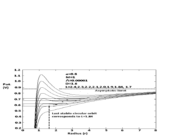
Figure 1: Potential-energy curves appropriate for time-like trajectories in Kerr-de Sitter space time.

2.2.2 Rotational velocity in time like trajectory

As in the Schwarzschild and the Reissner-Nordstrom geometric, the circular orbits play an important role in the classification of the orbits. Besides, they are useful in providing simple examples of orbits which exhibit the essential features at the same time; and this is, after all, the reason for studying the geodesics.

We seek then the values of $L$ and $E$ which a circular orbit at some assigned radius, $r=\frac{1}{u}$, will have. When $L$ and $E$ have these values, the cubic polynomial on the right-hand side of equation (2.2) will have a double root.
The conditions for the occurrence of a double root, after substituting $x=L-aE$ are,

$$\dot{r}^{2}r^{4}=f\,(r)=E^{2}r^{4}-r^{2}\Delta_{r}-2aEr^{2}x+(a^{2}-\Delta_{r})x^{2}=0$$ (36)

and differentiating equation (36) with respect to r

$$f^{\prime}\,(r)=4E^{2}r^{3}-2r\Delta_{r}-r^{2}{\Delta_{r}}^{\prime}-4aErx-{\Delta_{r}}^{\prime}x^{2}=0$$ (37)

Equations (36) and (37) can be written to give

$$E^{2}r^{4}-\frac{r^{3}}{2}{\Delta_{r}}^{\prime}+(\Delta_{r}-a^{2}-\frac{r}{2}{\Delta_{r}}^{\prime})x^{2}=0$$ (38)

$$E=\frac{1}{2ar^{2}x}\Big{[}(2a^{2}-2\Delta_{r}+\frac{r{\Delta_{r}}^{\prime}}{2})x^{2}+\frac{r^{3}}{2}{\Delta_{r}}^{\prime}-r^{2}\Delta_{r}\Big{]}$$ (39)

after substituting this value of $E$ in previous equation we get,

$$\Big{[}4a^{2}(\Delta_{r}-a^{2}-\frac{r}{2}{\Delta_{r}}^{\prime})+(2a^{2}-2\Delta_{r}+\frac{r}{2}{\Delta_{r}}^{\prime})^{2}\Big{]}x^{4}+\Big{[}2(2a^{2}-2\Delta_{r}+\frac{r}{2}{\Delta_{r}}^{\prime})(\frac{r^{3}}{3}{\Delta_{r}}^{\prime}$$

$$-r^{2}\Delta_{r})-2a^{2}r^{3}{\Delta_{r}}^{\prime}\Big{]}x^{2}+\big{(}\frac{r^{3}}{2}{\Delta_{r}}^{\prime}-r^{2}\Delta_{r}\big{)}^{2}=0\quad$$ (40)

which is in the form of quadratic equation in $x^{2}$ i.e.

$$a(x^{2})^{2}+b(x^{2})+c$$

The discriminant $\frac{b^{2}-4\,a\,c}{4}$ of this equation is

$$8a^{2}r^{4}\Delta_{r}^{2}[a^{2}-\Delta_{r}+\frac{r}{2}{\Delta_{r}}^{\prime}]$$

Thus we can find solution of equation (2.2.2) as

$$x^{2}=\frac{r^{2}\bigg{(}a\pm\sqrt{a^{2}-\Delta_{r}+\frac{r}{2}{\Delta_{r}}^{\prime}}\bigg{)}^{2}}{\bigg{(}2\Delta_{r}-2a^{2}-\frac{r}{2}{\Delta_{r}}^{\prime}\bigg{)}\mp 2a\sqrt{a^{2}-\Delta_{r}+\frac{r}{2}{\Delta_{r}}^{\prime}}}$$ (41)

where,

$$\bigg{(}2\Delta_{r}-2a^{2}-\frac{r}{2}{\Delta_{r}}^{\prime}\bigg{)}-4a^{2}\bigg{(}a^{2}-\Delta_{r}+\frac{r}{2}{\Delta_{r}}^{\prime}\bigg{)}=Q_{+}\,Q_{-}$$

and

$$Q_{\pm}=\bigg{(}2\Delta_{r}-2a^{2}-\frac{r}{2}{\Delta_{r}}^{\prime}\bigg{)}\pm 2a\sqrt{a^{2}-\Delta_{r}+\frac{r}{2}{\Delta_{r}}^{\prime}}$$ (42)

Therefore,

$$x^{2}=\frac{r^{2}(\Delta_{r}-Q_{\mp})}{Q_{\mp}}$$ (43)

From equations (41) and (42) the solution for $x$ thus takes the simple form

$$x=-\frac{r}{\sqrt{Q_{\mp}}}\bigg{(}a\pm\sqrt{a^{2}-\Delta_{r}+\frac{r}{2}{\Delta_{r}}^{\prime}}\bigg{)}=\frac{r}{2a\sqrt{Q_{\mp}}}\big{(}\frac{r}{2}{\Delta_{r}}^{\prime}-2\Delta_{r}+Q_{\mp}\big{)}$$ (44)

The upper sign in the equations apply to retrograde orbits and lower sign apply to direct orbits.
Using value of $x$ in equation (38),

$$E=\frac{1}{r\sqrt{Q_{\mp}}}\bigg{(}\Delta_{r}-a^{2}\mp a\sqrt{a^{2}-\Delta_{r}+\frac{r}{2}{\Delta_{r}}^{\prime}}\bigg{)}=\frac{1}{2r\sqrt{Q_{\mp}}}\big{(}\frac{r}{2}{\Delta_{r}}^{\prime}+Q_{\mp}\big{)}$$ (45)

and thus, $L=aE+x$ i,e;

$$L=\frac{1}{r\sqrt{Q_{\mp}}}\bigg{[}a(\Delta_{r}-a^{2}-r^{2})\mp(a^{2}+r^{2})\sqrt{a^{2}-\Delta_{r}+\frac{r}{2}{\Delta_{r}}^{\prime}}\,\bigg{]}$$ (46)

Here $E$ and $L$ are the energy and the angular momentum per unit mass, of a particle describing a circular orbit of reciprocal radius $u$.

Now, using the values of $L$, $x$ and $E$ to find velocity of test particle, we know

$$\Omega=\frac{d\phi}{dt}=\frac{\dot{\phi}}{\dot{t}}=\frac{\mp\sqrt{a^{2}-\Delta_{r}+\frac{r}{2}{\Delta_{r}}^{\prime}}}{\Big{(}r^{2}\mp a\sqrt{a^{2}-\Delta_{r}+\frac{r}{2}{\Delta_{r}}^{\prime}}\Big{)}}$$

and

$$\omega=\frac{a}{\Sigma^{2}}\big{[}(r^{2}+a^{2})\Delta_{\theta}-\Delta_{r}\big{]}$$

where $\Sigma^{2}=(r^{2}+a^{2})^{2}\Delta_{\theta}-\Delta_{r}a^{2}sin^{2}\theta$

The rotational velocity of test particle in the orbit around the central mass is

$$V_{\varphi}=\frac{\Sigma^{2}sin^{2}\theta}{\rho^{2}\sqrt{\Delta_{r}\Delta_{\theta}}}(\Omega-\omega)$$

Thus, using these values rotational velocity we obtained as

$$V_{\varphi}=\mp\frac{\bigg{[}\big{(}r^{2}+a^{2}\big{)}\sqrt{a^{2}-\Delta_{r}+\frac{r}{2}{\Delta_{r}}^{\prime}}\pm a\big{(}r^{2}+a^{2}-\Delta_{r}\big{)}\bigg{]}}{\big{(}r^{2}\mp a\sqrt{a^{2}-\Delta_{r}+\frac{r}{2}{\Delta_{r}}^{\prime}}\big{)}\sqrt{\Delta_{r}}}$$ (47)

In the limit $\Lambda\longrightarrow 0$

$$V_{\varphi}=\mp\frac{\sqrt{\frac{M}{r}}\Big{[}1+\frac{a^{2}}{r^{2}}\pm\frac{2a}{r}\sqrt{\frac{M}{r}}\Big{]}}{\Big{[}1\mp\frac{a}{r}\sqrt{\frac{M}{r}}\Big{]}\Big{[}1+\frac{a^{2}}{r^{2}}-\frac{2M}{r}\Big{]}^{1/2}}$$ (48)

which is for Kerr space-time metric.
Similarly, in the limit $a\longrightarrow 0$,

$$V_{\varphi}=\sqrt{\frac{\frac{M}{r}-\frac{\Lambda r^{2}}{3}}{1-\frac{2M}{r}-\frac{\Lambda r^{2}}{3}}}$$ (49)

Which is the Schwarzschild de-Sitter limit.

When $\frac{M}{r}<<1$, equation (49) reduces to the usual Newtonian limit, with $G$ = $c$ = 1,

$$V_{\varphi}=(\frac{M}{r})^{\frac{1}{2}}$$

i.e;

$$V_{\varphi}=(\frac{G\,M}{c^{2}\,r})^{\frac{1}{2}}$$

3 Analysis of geodesic motion in Kerr-de Sitter space-time

The time-like geodesics motion in Kerr-de Sitter space-time is one of the complicated problem. The equation of motion in circular orbit is a non linear. It has distance from center as independent parameter and velocity as dependent parameter. It contains mass, cosmological constant and angular momentum or spinning constant or rotational Kerr parameter as constant parameters. For different values of mass, cosmological constant and Kerr parameter; nature of geodesic motion can be displayed which are as follows:

1)The rotational velocity increases with mass (M) keeping cosmological constant non-negative. For non-negative value of $\Lambda$; ‘$v$’ vs ‘$r$’ curves do not meet to each other while they meet after a certain point for negative value of $\Lambda$. The value of meeting point depends upon the value of $\Lambda$. The plots of ‘$v$’ vs ‘$r$’ curves are shown in fig. 2.

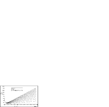
Figure 2: First two figures show geodesic curves for different values of mass keeping constant value of $a$ and constant positive and negative values of $\Lambda$ respectively while that of last two show geodesic curves of positive and negative variation of $\Lambda$ respectively with constant value of $M$ and $a$

2)The curvature is dependent on value of $\Lambda$. For non negative value of $\Lambda$ velocity decreases as distance increases while velocity increases with distance for negative value of $\Lambda$ keeping mass constant. The plot showing different curves due to the variation of $\Lambda$ is shown in fig. 2.

3)Since $a$ appears as multiplicative factor with mass (M) and lies in the range 0.1 $-$ 1.0, its effect in curvature is found to be negligible as shown in fig. 3.

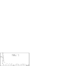
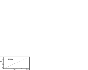
Figure 3: Geodesic curves with variation of $a$ with constant positive and negative value of $\Lambda$ and constant value of $M$.

4 Application of geodesic motion in Kerr-de Sitter space-time

In this section we intend whether geodesic motion in Kerr-de Sitter space-time could be applied or not. So, we focused our interest to the database of rotational curves data of galaxies which were well fitted to our problems. For this we took non-linear curve fit statistics for which R-square and adjusted R-square errors in such a way that it should be non negative. We selected 30 galaxies and fitted the values of mass (M), cosmological constant ($\Lambda$) and rotational Kerr parameter ($a$). Among 30 galaxies, the values of rotational velocity ($v$) and the distance from the galactic center ($r$) for 28 galaxies are taken from the database provided by Sofue et al. (2007) and that for the rest 2 galaxies (NGC 3379 and NGC 4100) are taken from the data digitized by Software ‘Labfit’ from the literatures of Brownstein & Moffat (2005). We used software Matlab7.6 to carry out non-liner least square curve fit method to estimate the values of M, $\Lambda$ and $a$. In this parametric curve fitting M, $\Lambda$ and $a$ were obtained as unknown coefficients from our equation of motion.

Out of 30 galaxies we could fit positive cosmological constant for 23 galaxies while it was negative for 7 galaxies. To find the unknown parameters we analyzed the nature of curve of equation of motion in Kerr-de Sitter space-time and fitted with rotation curves data of galaxies. As discussed in above section, it is found that the rotational velocity in the flat portion in the rotation curves data of galaxies increases with mass (M) keeping $\Lambda$ non negative. Similarly, curvature is found to be dependent on the value of $\Lambda$. For non negative value of $\Lambda$ velocity decreases as distance increases while for negative value it increases as distance increases keeping mass constant. We found value of $a$ has negligible contribution in the curvature but it affects in goodness of fit statistics. So we minimized the errors associated with it. Thus we fitted rotation curves data for most appropriate values of mass (M), cosmological constant ($\Lambda$) and Kerr parameter ($a$).

The value of cosmological constant is found to lie within the range of $\rm(1.790\pm 0.286)\times 10^{-49}\,\,km^{-2}$ to $\rm(7.523\pm 1.204)\times 10^{-42}\,\,km^{-2}$ for positive value of $\Lambda$ while $\rm-(3.983\pm 0.637)\times 10^{-41}\,\,km^{-2}$ to $\rm-(1.860\pm 0.298)\times 10^{-42}\,\,km^{-2}$ for negative value of $\Lambda$. Among positive values the least value is found for the galaxy NGC 3521 and maximum is found for the galaxy NGC 3034. Similarly, among negative values maximum is found for NGC 2708 and minimum value value is found for NGC 3495. Negative cosmological constants were found to fit for the galaxies which are high red shifted spiral galaxies. Exception to these is NGC 4569 which is high blue shifted having radial velocity equals -235 km/s. This is found to be Sab morphological type and having LINER activity. Galaxies having low value of radial velocities ($\sim$ -300 km/s to 1116 km/s) were found to fit with positive cosmological constants. Exception to these are NGC 1097, NGC 1365, NGC 4321 and NGC 4565 ($\sim$ 1230 km/s to 1636 km/s). We have found greater value ($\rm\sim 10^{-42}\,\,km^{-2}$ to $\rm 10^{-47}\,\,km^{-2}$) of cosmological constants for galaxies NGC 1808, NGC 3034, NGC 3521, NGC 4736 and NGC 5194. Out of which NGC 1808, NGC 3034 are found to be of active galaxies and NGC 5194 (M51) shows peculiar characteristics (Sofue et al., 1999). While NGC 4736 is found to be of Sab type and having radial velocity equals 606 km/s. In general, we found cosmological constant in the range of $\rm 10^{-41}\,\,km^{-2}$ to $\rm 10^{-49}\,\,km^{-2}$ for positive value of cosmological constant and in the range of $-\rm 10^{-41}\,\,km^{-2}$ to $\rm-10^{-42}\,\,km^{-2}$ for negative value of $\Lambda$ which are in agreement with the values found in other literatures.

The estimated mass of the galaxies lie in the range of $\rm(0.12\pm 0.02)\times 10^{10}\,\,M_{\odot}$ to $\rm(70.37\pm 11.26)\times 10^{10}\,\,M_{\odot}$ where $\rm 1M_{\odot}=1.989\times 10^{30}$ kg which are also in good agreement with other estimated values found in literatures. Value of mass is found small $\rm(0.73\pm 0.12)\times 10^{10}\,\,M_{\odot}$ for NGC 3034 which is Ir II type and have positive value of $\Lambda$. While value of mass $\rm(0.12\pm 0.02)\times 10^{10}\,\,M_{\odot}$) is found for NGC 3495 which is Sd type and have negative cosmological constant. Greater value of mass is found for NGC 1097 which is of SBb type. We had also calculated mass of elliptical galaxy NGC 3379 whose value is found to fit with $\rm(1.027\pm 0.164)\times 10^{11}\,\,M_{\odot}$. In general mass is found to lie in the range $\rm 10^{9}\,\,M_{\odot}$ to $\rm 10^{11}\,\,M_{\odot}$ for spiral barred and unbarred galaxies.

Similarly value of Kerr parameter we fitted lie in the range of (0.7044$\pm$0.1127) to (0.9990$\pm$0.1598). These are the values that could have minimum error in non-linear least square curve fitting. Small value (0.7044$\pm$0.1127) of $a$ is found for NGC 4736 which is early type barred spiral (Sab) type and it has small mass while greater value (0.9990$\pm$0.1598) is found for NGC 3379 which is of elliptical type. Recent measurements of the Kerr parameters $a$ for two stellar sized black-hole binaries in our Galaxy (Shafee et al. 2006) for GRO J1655-40 and 4U 1543-47 are estimated to fall in the range $a=0.65-0.75$ and $a=0.75-0.85$, respectively. Our estimated values are quite reasonable because we know that spin angular momentum for a collective mass of the galaxy has always higher value than for a black hole mass. We found most of our estimated massive galaxies ($>50\%$) are fitted with the higher value of $a$. Since spin of barred and unbarred galaxies not only mass dependent but also depends on their local inner activities such as starbursts as well as globular cause such as its neighbouring galaxies, its position in galaxy cluster etc. These results might be interesting in the future studies.

The best fitted graph of some galaxies are shown in fig.(5). The detailed best fitted values of mass (M), cosmological constant ($\Lambda$), Kerr parameter ($a$) and errors associated with it are given in Table (1).

Table 1: Estimated values of Mass (M), Cosmological Constant $\Lambda$ and Kerr Parameter ($a$) for different Galaxies

Name Of Galaxy	Mass $\rm(M_{\odot})$	Mass In kg	Cosmological Constant $\Lambda$ (km-2)	Kerr Parameter ($a$)	SSE	R- Square Error	Adjusted R-Squared Error	RMSE
NGC0224	(39.05$\pm$6.25)$\times$1010	(7.767$\pm$1.242)$\times$1041	(2.339$\pm$0.374)$\times$10-48	(0.9900$\pm$0.1584)	91319.635	0.3090	0.3090	13.190
NGC0891	(18.88$\pm$3.02)$\times$1010	(3.755$\pm$0.601)$\times$1041	(2.337$\pm$0.374)$\times$10-48	(0.7800$\pm$0.1248)	14462.815	0.9472	0.9472	6.021
NGC1097	(70.37$\pm$11.26)$\times$1010	(13.996$\pm$2.239)$\times$1041	(2.331$\pm$0.373)$\times$10-48	(0.8900$\pm$0.1424)	25440.000	0.0427	0.0427	10.520
NGC1365	(43.36$\pm$6.94)$\times$1010	(8.624$\pm$1.380)$\times$1041	(5.023$\pm$0.804)$\times$10-49	(0.7980$\pm$0.1277)	17726.015	0.0165	0.0165	8.704
NGC1808	(9.55$\pm$1.53)$\times$1010	(1.899$\pm$0.304)$\times$1041	(2.020$\pm$0.323)$\times$10-47	(0.8809$\pm$0.1409)	31935.047	0.7259	0.7359	11.990
NGC2683	(11.69$\pm$1.87)$\times$1010	(2.325$\pm$0.372)$\times$1041	(2.330$\pm$0.373)$\times$10-48	(0.8600$\pm$0.1376)	855.955	0.2592	0.2592	13.310
NGC2903	(25.04$\pm$4.01)$\times$1010	(4.980$\pm$0.797)$\times$1041	(2.278$\pm$0.364)$\times$10-48	(0.7721$\pm$0.1235)	840.200	0.8869	0.8863	2.191
NGC3031	(16.06$\pm$2.56)$\times$1010	(3.194$\pm$0.511)$\times$1041	(2.337$\pm$0.374)$\times$10-48	(0.9500$\pm$0.1520)	53039.950	0.7400	0.7400	12.850
NGC3034	(0.73$\pm$0.12)$\times$1010	(0.145$\pm$0.023)$\times$1041	(7.523$\pm$1.204)$\times$10-42	(0.9530$\pm$0.1525)	2429.588	0.9843	0.9843	5.934
NGC3079	(21.76$\pm$3.48)$\times$1010	(4.328$\pm$0.692)$\times$1041	(4.100$\pm$0.656)$\times$10-49	(0.9600$\pm$0.1536)	16568.786	0.8425	0.8425	7.107
NGC3379	(10.27$\pm$1.64)$\times$1010	(2.043$\pm$0.327)$\times$1041	(2.220$\pm$0.355)$\times$10-48	(0.9990$\pm$0.1598)	12077.879	0.0494	0.0494	25.900
NGC3521	(21.76$\pm$3.48)$\times$1010	(4.328$\pm$0.692)$\times$1041	(1.790$\pm$0.286)$\times$10-49	(0.8720$\pm$0.1395)	63070.305	0.0430	0.0430	15.090
NGC3628	(18.65$\pm$2.98)$\times$1010	(3.709$\pm$0.593)$\times$1041	(2.221$\pm$0.355)$\times$10-48	(0.8200$\pm$0.1312)	14779.169	0.0639	0.0556	11.490
NGC4100	(13.96$\pm$2.23)$\times$1010	(2.776$\pm$0.444)$\times$1041	(3.130$\pm$0.501)$\times$10-48	(0.8800$\pm$0.1408)	1390.000	0.0424	0.0424	10.760
NGC4321	(46.55$\pm$7.45)$\times$1010	(9.259$\pm$1.481)$\times$1041	(3.220$\pm$0.516)$\times$10-48	(0.7974$\pm$0.1276)	29804.774	0.0282	0.2352	12.030
NGC4565	(49.47$\pm$7.92)$\times$1010	(9.839$\pm$1.574)$\times$1041	(2.342$\pm$0.375)$\times$10-48	(0.8200$\pm$0.1312)	8539.000	0.9013	0.9013	2.729
NGC4631	(16.12$\pm$2.58)$\times$1010	(3.206$\pm$0.513)$\times$1041	(2.338$\pm$0.374)$\times$10-48	(0.7410$\pm$0.1186)	2559.000	0.9633	0.9633	2.729
NGC4736	(6.89$\pm$1.10)$\times$1010	(1.370$\pm$0.219)$\times$1041	(1.242$\pm$0.198)$\times$10-42	(0.7044$\pm$0.1127)	128.300	0.9969	0.9969	1.095
NGC5033	(61.73$\pm$9.88)$\times$1010	(12.228$\pm$1.956)$\times$1041	(7.640$\pm$1.222)$\times$10-49	(0.8600$\pm$0.1376)	9858.784	0.7809	0.7809	4.952
NGC5194	(16.63$\pm$2.66)$\times$1010	(3.308$\pm$0.529)$\times$1041	(4.048$\pm$0.648)$\times$10-42	(0.7490$\pm$0.1198)	2300.000	0.9934	0.9934	3.700
NGC5236	(24.42$\pm$3.91)$\times$1010	(4.857$\pm$0.777)$\times$1041	(2.296$\pm$0.367)$\times$10-48	(0.7679$\pm$0.1228)	57164.049	0.0119	0.0097	11.090
NGC5457	(16.70$\pm$2.58)$\times$1010	(3.321$\pm$0.531)$\times$1041	(2.180$\pm$0.349)$\times$10-49	(0.7419$\pm$0.1187)	784.106	0.9766	0.9766	2.447
NGC5907	(41.23$\pm$6.59)$\times$1010	(8.200$\pm$1.312)$\times$1041	(2.347$\pm$0.375)$\times$10-48	(0.8600$\pm$0.1376)	3413.499	0.9643	0.9643	3.183
NGC2708	(30.76$\pm$4.92)$\times$1010	(6.118$\pm$0.979)$\times$1041	-(1.860$\pm$0.298)$\times$10-42	(0.7842$\pm$0.1255)	3893.188	0.8909	0.8909	2.556
NGC3495	(0.12$\pm$0.02)$\times$1010	(0.023$\pm$0.004)$\times$1041	-(3.983$\pm$0.637)$\times$10-41	(0.9100$\pm$0.1456)	15912.276	0.7329	0.7297	13.680
NGC3672	(4.08$\pm$0.65)$\times$1010	(0.811$\pm$0.129)$\times$1041	-(1.329$\pm$0.213)$\times$10-41	(0.8896$\pm$0.1423)	4407.277	0.9130	0.9130	4.742
NGC4303	(4.57$\pm$0.73)$\times$1010	(0.909$\pm$0.145)$\times$1041	-(3.450$\pm$0.552)$\times$10-42	(0.9900$\pm$0.1584)	383.910	0.3278	0.3225	1.739
NGC4569	(3.16$\pm$0.50)$\times$1010	(0.629$\pm$0.101)$\times$1041	-(3.970$\pm$0.635)$\times$10-41	(0.9860$\pm$0.1578)	3900.010	0.9247	0.9239	6.547
NGC6951	(5.04$\pm$0.81)$\times$1010	(1.002$\pm$0.160)$\times$1041	-(1.783$\pm$0.285)$\times$10-41	(0.8550$\pm$0.137)	3215.000	0.8449	0.8432	5.818
UGC3691	(0.40$\pm$0.06)$\times$1010	(0.079$\pm$0.012)$\times$1041	-(1.394$\pm$0.223)$\times$10-41	(0.9129$\pm$0.1461)	6228.231	0.8795	0.8795	7.031

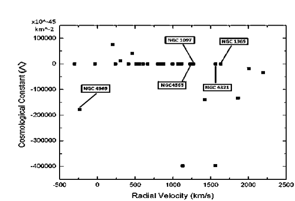
Figure 4: Plot diagram of $\Lambda$ vs Radial Velocity of galaxies. Each square box contains the name of galaxy having exceptional behaviour.

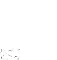
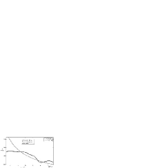
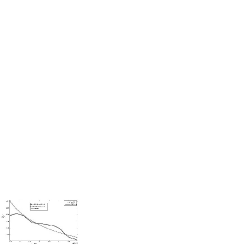
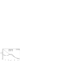
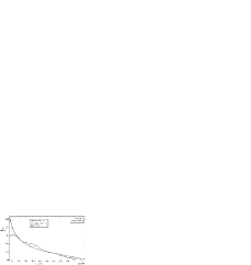
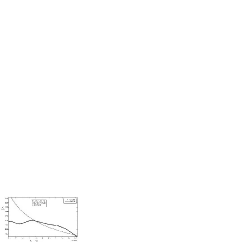
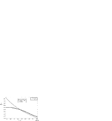
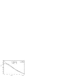
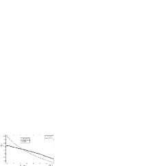
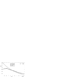
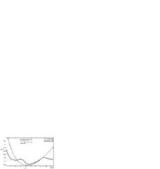
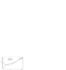
Figure 5: The observed and fitted rotation curves of galaxies NGC 0224, NGC 0891, NGC 1808, NGC 2903, NGC 3034, NGC 3079, NGC 4631, NGC 4736, NGC 5236, NGC 5907, NGC 2708 and UGC 3691.. The thick solid and thin solid curve represents the observed and fitted line respectively. The value of M, $\Lambda$ and $a$ is shown inside the square box.

5 Conclusion

For some typical values of the parameters $\Lambda$, $D$, $L$ and $a$ there exists a potential-energy curve. The minima in the potentials corresponds to the stable circular orbits while maxima corresponds to unstable circular orbits. At the point of inflection the last stable circular orbit occurs.

The value of the rotational velocity in the flat portion in the rotation curves data of galaxies is found to be increased with mass (M) keeping cosmological constant ($\Lambda$) non-negative. But, that for a constant negative value of $\Lambda$, ‘$v$’ vs ‘$r$’ curves meet after a certain distance. The meeting point is observed to be dependent on the value of $\Lambda$.

The Curvature of rotation curve data of Galaxies is found to be dependent on the value of $\Lambda$ keeping mass constant. For non negative value of $\Lambda$, velocity ($v$) decreases as distance from galactic center ($r$) increases while for negative value of $\Lambda$ velocity ($v$) increases as the distance increases. Thus $\Lambda$ is found to be a essential parameter to fit the curvature of rotation curves data of galaxies.

Since Kerr parameter lies in the range of 0.1 to 1.0 and appears as coefficient of mass in our equation of motion, it has negligible contribution in ‘$v$’ vs ‘$r$’ curve. But it has an effect in goodness of fit statistics, particularly in non-linear least square curve fitting.

The value of mass (M) of galaxies is estimated in the range of $\rm(0.12\pm 0.02)\times 10^{10}\,\,M_{\odot}$ to $\rm(70.37\pm 11.26)\times 10^{10}\,\,M_{\odot}$. NGC 1097 is found to be more massive than others which is of SBb type. Least mass $\rm(0.12\pm 0.02)\times 10^{10}M_{\odot}$ is found for NGC 3495 which is fitted for negative cosmological constant and is of Sd type. Value of mass is found small $\rm(0.73\pm 0.12)\times 10^{10}M_{\odot}$ for NGC 3495 which is Ir II type. In general mass is found to lie in the range $\rm 10^{9}\,\,M_{\odot}$ to $\rm 10^{11}\,\,M_{\odot}$ for spiral barred and unbarred galaxies.

The nature of cosmological constant fitted for galaxies were found to depend upon radial velocities of galaxies. Discarding exceptional cases, for the higher values of radial velocity cosmological constants were found to be negative while positive for small values of RV. This suggest some local phase transition effects at the time when the high redshift galaxies were formed.

The value of Cosmological Constant is found to fall within the range of $\rm(1.790\pm 0.286)\times 10^{-49}\,\,km^{-2}$ to $\rm(7.523\pm 1.204)\times 10^{-42}\,\,km^{-2}$ for positive value of $\Lambda$ while $\rm-(3.983\pm 0.637)\times 10^{-41}\,\,km^{-2}$ to $\rm-(1.860\pm 0.298)\times 10^{-42}\,\,km^{-2}$ for negative value of $\Lambda$. Most of the galaxies were fitted for the values of $\Lambda$ in the range of $\rm 10^{-49}\,\,km^{-2}$ to $\rm 10^{-48}\,\,km^{-2}$.

The value of Kerr parameter lies in the range of (0.7044$\pm$0.1127) to (0.9990$\pm$0.1598). Small value, i.e., (0.7044$\pm$0.1127) of $a$ is found for NGC 4736 which is Sab type galaxy. It has small mass while greater value (0.9990$\pm$0.1598) is found for NGC 3379 which is elliptical type.

6 Acknowledgement

We are indebted to all faculty members and students at Central Department of Physics, Tribhuvan University, Kirtipur for their constant helps and suggestions during the work. Specially, we would like to thank Mr. P. R. Dhungel for his kind support.

References

- [1] Akcay S., The Kerr-de Sitter Universe, (http://www.arXiv:astroph1011.0479v1), (2009)
- [2] Bhatta G. P., Null and Time-Like Geodesics in Kerr-Desitter Space Time, M.sc. Thesis (Physics), Trivuvan University, Kirtipur, (2001)
- [3] Brownstein J.R. & Moffat J.W., Galaxy Rotation Curves Without Non-Baryonic Dark Matter, arXiv: astro-ph0506370v4 (22 sep 2005)
- [4] Chandrasekhar S., The mathematical Theory of Black Holes, Oxford University Press, New York (1983)
- [5] Chandrasekhar S., The mathematical Theory of Black Holes, Oxford University Press, New York (1999)
- [6] Goldsmith D., Einstein’s Greatest Blunder: the Cosmological Constant, Havard University Press (1995)
- [7] Islam J. N., An Introduction to Mathematical Cosmology, Cambridge University Press, The Edinburgh Building, Cambridge (2004)
- [8] Jones B. & Saha P., The Galaxy, Notes for Lecture Courses ASTM002 and MAS430, Queen Mary University of London (2004)
- [9] Malakar N.K. & Khanal U., The null geodesics in Kerr-de Sitter Space-Time, Scientific World, Vol. 3, No. 3, (July 2005)
- [10] Moore, Sir Patrick, Phillip’s Atlas of Universe, Phillip’s Octopus Publishing Group Ltd. (2005)
- [11] Narlikar J., Introduction to Cosmology, Cambridge University Press, Cambridge (1993)
- [12] Pokhrel J., Geodesics in the Schwarzschild de-Sitter Space-time & Effect of the Cosmological Constant on Rotational and Infall Velocity, M. Sc. Thesis, Tribhuvan University, Kirtipur (1997)
- [13] Poudel P.C., B. Aryal & U. Khanal, Estimation of mass, cosmological constant and Kerr parameter of different galaxies using geodesic motion in Kerr-de Sitter space time, M.sc. Thesis (Physics), Trivuvan University, Kirtipur, (2011)
- [14] Robinson L. J., Philip’s Astronomy Encyclopedia, Philips Octopus Publishing Group (2002)
- [15] Sahai R., Bulletin of the American Astronomical Society, 34, 1142 (2002)
- [16] Sahani V.,The Physics of the Early Universe, Lect. Notes Phys. 653 (Springer, Berlin Heidelberg), DOI 10.1007/b99562 (2005)
- [17] Sofue Y., Tutui Y., Honma M., Tomita A., Takamiya T., Koda J., & Takeda Y., Central Rotational Curves Of Galaxies, The Astrophysical Journal, 523:136-146, (1999 September 20)
- [18] web1: http://nasa.gov/dark matter
- [19] web2: http://nasa.gov/dark energy
- [20] web3: http://zebu.uoregon.edu/ js/ast123/lectures/lec13.html (3 of 10) [15-02-2002 22:36:10]