Scalar masses in general N=2
gauged supergravity theories

Francesca Catino, Claudio A. Scrucca and Paul Smyth

Institut de Théorie des Phénomènes Physiques, EPFL,
CH-1015 Lausanne, Switzerland

We readdress the question of whether any universal upper bound exists on the square mass $m^{2}$ of the lightest scalar around a supersymmetry breaking vacuum in generic N=2 gauged supergravity theories for a given gravitino mass $m_{3/2}$ and cosmological constant $V$. We review the known bounds which apply to theories with restricted matter content from a new perspective. We then extend these results to theories with both hyper and vector multiplets and a gauging involving only one generator, for which we show that such a bound exists for both $V>0$ and $V<0$. We finally argue that there is no bound for the same theories with a gauging involving two or more generators. These results imply that in N=2 supergravity theories metastable de Sitter vacua with $V\ll m^{2}{}_{3/2}$ can only arise if at least two isometries are gauged, while those with $V\gg m^{2}{}_{3/2}$ can also arise when a single isometry is gauged.

1 Introduction

Spontaneous supersymmetry breaking in a vacuum that is at least metastable is notoriously difficult to achieve in N=2 supersymmetric theories. This is related to the very constrained structure of these theories, with a non-linear sigma-model involving target spaces with special geometries and potentials related to the gauging of some isometries on these manifolds. In the interesting case of theories that can be consistently coupled to gravity, several general results concerning the scalar masses in supersymmetry breaking vacua have been obtained, both for rigid and local supersymmetry. For theories with $n_{H}$ hypermultiplets and no vector multiplets, it was proven in [1] that at least one of the scalars must have square mass $m^{2}\leq-\,V-\frac{1}{3}\,m^{2}_{3/2}$. Similarly, for theories with $n_{V}$ Abelian vector multiplets and no hypermultiplets, it was shown in [2] (see also [3]) that the lightest scalar must have square mass $m^{2}\leq-2V$. These bounds apply to theories with local supersymmetry, with $V$ parametrizing the vacuum energy and $m_{3/2}$ denoting the gravitino mass, and imply that de Sitter vacua are necessarily unstable in those theories. They also have a non-trivial meaning in the rigid limit, in which they reduce to the statement that at least one scalar has $m^{2}\leq 0$, implying that non-supersymmetric vacua cannot be completely stable [4]. These universal results were derived by looking at the averaged sGoldstino mass, for which the dependence on the curvature of the scalar manifold turns out to drop out completely, contrary to what happens for N=1 theories [5, 6, 7] (see also [8, 11, 9, 10]) or even N=2 to N=1 truncated theories [12].

The aim of this work is to investigate whether there exists a similar bound on the mass of the lightest scalar in more general N=2 theories involving $n_{H}$ hypermultiplets and $n_{V}$ vector multiplets. Little is known so far about the systematics of supersymmetry breaking in these theories for general $n_{H}$ and $n_{V}$. However, the simplest case where $n_{H}=1$ and $n_{V}=1$ and a single isometry is gauged has been studied in full generality in [15] for rigid theories and then in [16] for local theories. Exploiting the fact that in such a situation it becomes possible to parametrize the scalar geometries of both sectors in a much more concrete way in terms of harmonic functions, it was shown that a sharp bound on the mass of the lightest scalar emerges in this case too. For theories with local supersymmetry, this now approximately reads $m^{2}\mathrel{\vbox{\hbox{$<$}\nointerlineskip\hbox{$\sim$}}}-\frac{1}{2}V+\frac{1}{4}V^{2}/m^{2}_{3/2}$ for $V>0$ and is given by similar simple expressions in various ranges of $V<0$, and shows that de Sitter vacua can be metastable for sufficiently large cosmological constant. For theories with rigid supersymmetry, the corresponding bound is best expressed as $m^{2}\leq M^{2}$, where $M$ denotes the vector mass, and allows non-supersymmetric vacua to be metastable. These universal results were derived by reducing the full five-dimensional scalar mass matrix to a two-dimensional one by suitably averaging over the three physical scalars in the hyper sector and the two scalars in the vector sector. It is then clear that this approach does not quite correspond to just looking at the averaged sGoldstino mass, but rather exploits to some extent the distinction between the hyper and vector sectors. It is then natural to wonder whether a similar bound also persists in theories with generic $n_{H}$ and $n_{V}$. We will prove that this is indeed the case if there is only one gauged isometry. However, we will then argue that as soon as there are two or more gauged isometries, no universal bound is left, or in other words $m^{2}<+\infty$. In all our analysis we shall focus for simplicity on theories with Abelian gaugings. But, it is clear a posteriori that this does not represent a true limitation in the reach of our conclusion, since non-Abelian gaugings necessarily involve at least two gauged isometries, with which it is already possible to avoid a bound with an Abelian gauging.

The rest of the paper is organized as follows. In section 2 we briefly review the general structure of N=2 gauged supergravity theories, focusing on Abelian gaugings. In section 3 and 4 we then review how the known universal bounds on the square mass of the lightest scalar arises in theories with only hyper multiplets and only vector multiplets, emphasizing the crucial features that allow us to get rid of any dependence on the curvature of the scalar manifold. In section 5 we derive a new universal bound for theories with both hyper and vector multiplets and a single gauged isometry. In section 6 we then study the case of theories with both hyper and vector multiplets and a more general gauging, and argue that as soon as two or more isometries are gauged there is no way to derive any universal bound that does not depend on the curvature of the scalar manifold, and that by adjusting such a curvature at the vacuum point under consideration one can in fact achieve arbitrarily large masses for all the scalars. Finally, in section 7 we summarize our main conclusions and their implications.

2 N=2 gauged supergravity

Let us consider a general N=2 gauged supergravity theory with $n_{H}$ hypermultiplets and $n_{V}$ vector multiplets, restricting for simplicity to Abelian symmetries and using Planck units. The $4\,n_{H}$ real scalars $q^{u}$ from the hypermultiplets span a quaternionic-Kähler manifold with metric $g_{uv}$ and three almost complex structures $J^{x}{}^{u}{\!}_{v}$ satisfying $J^{x}{}^{u}{\!}_{w}J^{y}{}^{w}{\!}_{v}=-\delta^{xy}\delta{}^{u}{\!}_{v}+\epsilon^{xyz}J^{z}{}^{u}{\!}_{v}$. The $n_{V}$ complex scalars $z^{i}$ from the vector multiplets span instead a projective special-Kähler manifold with metric $g_{i\bar{\jmath}}$ and complex structure $J{}^{i}{\!}_{j}=i\delta{}^{i}{\!}_{j}$. The graviphoton $A_{\mu}^{0}$ and the $n_{V}$ vectors $A_{\mu}^{a}$ from the vector multiplets, denoted altogether by $A_{\mu}^{A}$, have kinetic matrix $\gamma_{AB}=-{\rm Im}\,{\cal N}_{AB}$ and topological angles $\theta_{AB}={\rm Re}\,{\cal N}_{AB}$ in terms of the period matrix ${\cal N}_{AB}$ associated with the special-Kähler manifold. One can then use these to gauge $n_{G}\leq n_{V}+1$ isometries of the quaternionic-Kähler manifold, which are described by triholomorphic Killing vectors $k_{A}^{u}$ each admitting three Killing prepotentials $P_{A}^{x}$ defined by the relations $\nabla_{u}P^{x}_{A}=-J^{x}_{uv}k_{A}^{v}$ and satisfying the equivariance conditions $J^{x}_{uv}k^{u}_{A}k^{v}_{B}=-\text{\small$\frac{1}{2}$}\epsilon^{xyz}P^{y}_{A}P^{z}_{B}$. The scalar and vector kinetic energy is given by [17, 18, 19, 20, 21, 22, 23, 24, 25]:

$$T=-\text{\small$\frac{1}{4}$}\gamma_{AB}F^{A}_{\mu\nu}F^{B\mu\nu}\!+\text{\small$\frac{1}{4}$}\theta_{AB}F^{A}_{\mu\nu}\tilde{F}^{B\mu\nu}\!-\text{\small$\frac{1}{2}$}\hskip 1.0ptg_{uv}\hskip 1.0ptD_{\mu}q^{u}D^{\mu}q^{v}\!-g_{i\bar{\jmath}}\,\partial_{\mu}z^{i}\partial^{\mu}\bar{z}^{\bar{\jmath}}\,.$$ (2.1)

In this expression $F^{A}_{\mu\nu}=\partial_{\mu}A^{A}_{\nu}-\partial_{\nu}A^{A}_{\mu}$, $\tilde{F}^{A}_{\mu\nu}=\frac{1}{2}\epsilon_{\mu\nu\rho\sigma}F^{A\rho\sigma}$ and $D_{\mu}q^{u}=\partial_{\mu}q^{u}+k^{u}_{A}A^{A}_{\mu}$. The scalar potential is instead given by

$$V=2g_{uv}k_{A}^{u}k_{B}^{v}L^{A}\bar{L}^{B}+g^{i\bar{\jmath}}f_{i}^{A}\bar{f}_{\bar{\jmath}}^{B}P_{A}^{x}P_{B}^{x}-3P_{A}^{x}P_{B}^{x}L^{A}\bar{L}^{B}\,.$$ (2.2)

Here $L^{A}$ denotes a generic covariantly holomorphic symplectic section of the special-Kähler manifold and $f_{i}^{A}=\nabla_{i}L^{A}$. Notice that the two $(n_{V}+1)\times(n_{V}+1)$ matrices $g^{i\bar{\jmath}}f_{i}^{A}\bar{f}_{\bar{\jmath}}^{B}$ and $P_{A}^{x}P_{B}^{x}$ are both positive definite. But since the $A,B$ indices run over $n_{V}+1$ values, while the indices $i,j$ run only over $n_{V}$ values and the indices $x,y$ only over $3$ values, the first is always singular with $1$ null vector and the second is singular whenever $n_{V}>3$ with $n_{V}-3$ null vectors. Finally, let us also recall that the average gravitino mass is given by

$$m^{2}_{3/2}=P_{A}^{x}P_{B}^{x}L^{A}\bar{L}^{B}\,.$$ (2.3)

The gauge symmetries are generically all spontaneously broken through the VEVs of the scalar transformation laws. The latter involve the Killing vectors $k^{u}_{A}$, and the order parameters of symmetry breaking are described by the matrix of scalar products of these vectors, which is recognized to be the vector mass matrix:

$$M^{2}_{AB}=2g_{uv}k_{A}^{u}k_{B}^{v}\,.$$ (2.4)

Supersymmetry is also generically completely broken through the VEVs of the hyperini and gaugini transformation laws. These involve the vectors $N_{u}^{x}=|\nabla_{u}P_{A}^{x}L^{A}|$ and $W_{i}^{x}=f_{i}^{A}P_{A}^{x}$ in the two sectors, respectively, and the order parameter of supersymmetry breaking is described by the sum of the norms of these two vectors, which is recognized to be the positive definite part of the potential, namely $V+3\hskip 1.0ptm^{2}_{3/2}=\frac{2}{3}g^{uv}N_{u}^{x}N_{v}^{x}+g^{i\bar{\jmath}}W_{i}^{x}\bar{W}_{\bar{\jmath}}^{x}$.

The quaternionic-Kähler manifold describing the hypermultiplet sector has holonomy $SU(2)\times SP(2n_{H})$ and a curvature tensor that can be parametrized by a four-index tensor $\Sigma_{urvs}$ enjoying some special properties:

$$R_{urvs}=-\text{\small$\frac{1}{2}$}\big{(}g_{u[v}g_{rs]}+J^{x}_{ur}J^{x}_{vs}+J^{x}_{u[v}J^{x}_{rs]}\big{)}+\Sigma_{urvs}\,.$$ (2.5)

The tensor $\Sigma_{urvs}$ has the same symmetry properties as the Riemann tensor, but is restricted to take the general form $\Sigma_{urvs}=\epsilon_{\Theta\Lambda}\epsilon_{\Pi\Psi}\,{\cal U}_{u}^{\Theta\theta}{\cal U}_{r}^{\Lambda\lambda}{\cal U}_{v}^{\Pi\pi}{\cal U}_{s}^{\Psi\psi}\Sigma_{\theta\lambda\pi\psi}$, where ${\cal U}^{\Theta\theta}_{u}$ denotes the vielbein, $\epsilon_{\Theta\Lambda}$ is the antisymmetric symbol of $SU(2)$ and $\Sigma_{\theta\lambda\pi\psi}$ is an arbitrary completely symmetric $SP(2n_{H})$ tensor. As a result of its very special form, $\Sigma_{urvs}$ gives a very restricted, specific contribution to the curvature. Firstly, it does not contribute to the contractions defining the Ricci and the scalar curvature, which are thus completely fixed and given by

$$R_{uv}=-(n_{H}+2)g_{uv}\,,\;\;R=-4n_{H}(n_{H}+2)\,.$$ (2.6)

Secondly, it also does not contribute to the completely symmetric part of the Riemannian curvature contracted with the sum of the product of two complex structures. Indeed, the complex structure can be rewritten as $J^{x}_{uv}=i\sigma^{x}_{\Theta\Lambda}c_{\theta\lambda}\,{\cal U}_{u}^{\Theta\theta}{\cal U}_{v}^{\Lambda\lambda}$, where $c_{\theta\lambda}$ denotes the antisymmetric symbol of $SP(2n_{H})$, and using the property $\sigma^{x}_{\Theta\Lambda}\sigma^{x}_{\Pi\Psi}=-2\hskip 1.0pt\epsilon_{\Theta(\Pi}\epsilon_{\Lambda\Psi)}$ one finds that the following quantity is completely fixed:

$$R_{(urvs}J^{x}{}^{r}{\!}_{p}J^{x}{}^{s}{\!}_{q)}=-3\hskip 1.0ptg_{(uv}g_{pq)}\,.$$ (2.7)

The special-Kähler manifold describing the vector multiplet sector has instead a curvature tensor that can be entirely characterized by a three-index tensor $C_{ijk}$ enjoying some special properties:

$$R_{i\bar{\jmath}p\bar{q}}=g_{i\bar{\jmath}}g_{p\bar{q}}+g_{i\bar{q}}g_{p\bar{\jmath}}-C_{ipr}g^{r\bar{s}}\bar{C}_{\bar{\jmath}\bar{q}\bar{s}}\,.$$ (2.8)

The tensor $C_{ijk}$ must be completely symmetric and covariantly holomorphic, but is otherwise arbitrary. It also controls the second covariant derivatives of the symplectic section, which read:

$$\nabla_{i}f_{j}^{A}=C_{ijk}\bar{f}^{kA}\,,\;\;\nabla_{i}\bar{f}_{\bar{\jmath}}^{A}=g_{i\bar{\jmath}}\bar{L}^{A}\,.$$ (2.9)

A supersymmetry breaking vacuum is generically associated to a point on the scalar manifold at which $V>-3\hskip 3.0ptm^{2}_{3/2}$ and $V^{\prime}=0$, and the mass matrix for scalar fluctuations is then related to the value of the Hessian matrix $V^{\prime\prime}$ at such a point. To explore the existence of possible obstructions to making all the scalars arbitrarily heavy by adjusting the parameters of the theory, one may choose an arbitrary point on the scalar manifold with fixed values of $V$ and $m^{2}_{3/2}$ and impose the stationarity conditions. The latter are then viewed as restrictions on the parameters of the theory, ensuring that the point under consideration is indeed a good vacuum. One then computes the scalar mass matrix and checks whether its eigenvalues can be made arbitrarily large or not whilst obeying the previous constraints. The general strategy to look for a non-trivial bound is then to study the scalar mass matrix along the particular directions in field space defined by the shift vectors $N_{u}^{x}=|\nabla_{u}P_{A}^{x}L^{A}|$ and $W_{i}^{x}=f_{i}^{A}P_{A}^{x}$, which determine the sGoldstino directions and are well defined under the assumption that supersymmetry is spontaneously broken both in the hyper and the vector sectors. By suitably averaging over all such directions, one may finally derive a single universal bound in units of $m^{2}_{3/2}$, which will depend on the following parameter controlling the cosmological constant $V$:

$$\epsilon=\frac{V}{m^{2}_{3/2}}\,.$$ (2.10)

Recall, finally, that vacuum metastability requires scalar masses to satisfy $m^{2}>0$ in de Sitter vacua with $\epsilon\in(0,+\infty)$ and $m^{2}>\frac{3}{4}\epsilon\hskip 1.0ptm^{2}_{3/2}$ in anti-de Sitter vacua with $\epsilon\in(-3,0)$.

3 Only hypers

Let us first briefly review the case of theories with $n_{H}$ hypers and no vectors with a gauging involving just the graviphoton, following [1]. In this case, $L^{0}$ is a constant. We can then define $k^{u}=k^{u}_{0}|L^{0}|$ and $P^{x}=P^{x}_{0}|L^{0}|$. In this way, the potential reads:

$$V=2\hskip 1.0ptk^{w}k_{w}-3\hskip 1.0ptP^{z}P^{z}\,.$$ (3.1)

The stationarity condition is obtained by computing the first covariant derivative and setting it to zero. This yields:

$$4\hskip 1.0ptk^{w}\nabla_{u}k_{w}-6\hskip 1.0ptP^{z}\nabla_{u}P^{z}=0\,.$$ (3.2)

The unnormalized scalar mass matrix is then defined by the second covariant derivative evaluated at the stationary point under consideration and reads:

$$m^{2}_{uv}=-4\big{(}R_{urvs}k^{r}k^{s}-\nabla_{u}k^{w}\nabla_{v}k_{w}\big{)}-6\big{(}P^{z}\nabla_{u}\nabla_{v}P^{z}+\nabla_{u}P^{z}\nabla_{v}P^{z}\big{)}\,.$$ (3.3)

The gravitino mass is instead given by:

$$m^{2}_{3/2}=P^{z}P^{z}\,.$$ (3.4)

One may now look at the mass matrix along the special set of vectors $N_{u}^{x}=\nabla_{u}P^{x}$ defining the sGoldstino directions, or equivalently

$$n^{ux}=\frac{\nabla^{u}P^{x}}{\sqrt{k^{w}k_{w}}}=-J^{x}{}^{u}{}_{v}\frac{k^{v}}{\sqrt{k^{w}k_{w}}}\,.$$ (3.5)

These are orthonormal with respect to the metric and satisfy $g_{uv}n^{ux}n^{vy}=\delta^{xy}$. One may then consider the following quantity, corresponding to the physical average sGoldstino mass:

$$m^{2}_{\rm bound}\equiv\text{\small$\frac{1}{3}$}m^{2}_{uv}n^{xu}n^{xv}\,.$$ (3.6)

This quantity $m^{2}_{\rm bound}$ represents by construction an upper bound on the square mass of the lightest scalar, and also a lower bound on that of the heaviest. Indeed, for each fixed $x=1,2,3$ the quantity $m^{2}_{uv}n^{xu}n^{xv}$ (no sum over $x$) is a normalized combination of the eigenvalues of the matrix $m^{2}_{uv}$ yielding its value along the unit vector $n^{x}_{u}$, which manifestly provides such type of bounds. The quantity $\text{\small$\frac{1}{3}$}m^{2}_{uv}n^{xu}n^{xv}$ (sum over $x$) then corresponds to the average of the above quantities over $x=1,2,3$, and thus also provides such type of bounds.

To evaluate more concretely the form of $m^{2}_{\rm bound}$, let us parametrize the potential $V$ in terms of the gravitino mass $m^{2}_{3/2}$ as

$$V=(x-3)m^{2}_{3/2}\,,$$ (3.7)

with

$$x=\frac{2k^{w}k_{w}}{P^{z}P^{z}}\,.$$ (3.8)

By using the stationarity condition (3.2) (which is easily shown to imply that $\nabla_{u}k^{w}n^{ux}=\frac{1}{2}(\delta^{xy}J^{z}{}^{w}{\!}_{u}+\epsilon^{xyz}\delta^{w}{\!\!\!}_{u})P^{y}n^{uz}$) and the special property (2.7) for the curvature, we then see that all the dependence on the curvature drops out and $m^{2}_{\rm bound}$ is found to be given by the following universal value:

$$m^{2}_{\rm bound}=\text{\small$\frac{1}{3}$}\big{(}8-3\hskip 1.0ptx\big{)}m^{2}_{3/2}\,.$$ (3.9)

We can finally rewrite the above result in terms of the dimensionless parameter $\epsilon$ defined in (2.10), which controls the cosmological constant. One simply has $x=3+\epsilon$, and therefore:

$$m^{2}_{\rm bound}=-\text{\small$\frac{1}{3}$}\big{(}1+3\hskip 1.0pt\epsilon\big{)}m^{2}_{3/2}\,.$$ (3.10)

In terms of $V$ and $m^{2}_{3/2}$, this finally means:

$$m^{2}_{\rm bound}=-\,V-\text{\small$\frac{1}{3}$}m^{2}_{3/2}\,.$$ (3.11)

This result shows that within this class of N=2 theories, de Sitter vacua are unavoidably unstable for any positive value $V>0$ of the cosmological constant, while anti-de Sitter vacua can be metastable only for sufficiently negative values $V\in(-3\hskip 1.0ptm^{2}_{3/2},-\frac{4}{21}\hskip 1.0ptm^{2}_{3/2})$ of the cosmological constant [1].

4 Only vectors

Let us next briefly review also the case of theories with $n_{V}$ vector multiplets with constant Fayet-Iliopoulos terms and no hypers, following [3]. In this case, the equivariance conditions force all the $P^{x}_{A}$, seen as $n_{V}$ tridimensional vectors, to be parallel. We can then write $P^{x}_{A}=\xi_{A}v^{x}$ with $v^{x}v^{x}=1$, and define $L=\xi_{A}L^{A}$ and $f_{i}=\xi_{A}f_{i}^{A}$. In this way, the potential becomes

$$V=\bar{f}^{k}f_{k}-3\hskip 1.0pt|L|^{2}\,,$$ (4.1)

and the stationarity condition reads

$$C_{ikl}\bar{f}^{k}\bar{f}^{l}-2\hskip 1.0ptf_{i}\bar{L}=0\,.$$ (4.2)

The Hermitian block of the unnormalized scalar mass matrix is then defined by the second mixed covariant derivatives evaluated at the stationary point under consideration and reads:

$$m^{2}_{i\bar{\jmath}}=-2\hskip 1.0ptR_{i\bar{\jmath}p\bar{q}}\bar{f}^{p}f^{\bar{q}}+2\hskip 1.0ptg_{i\bar{\jmath}}\big{(}\bar{f}^{k}f_{k}-|L|^{2}\big{)}\,.$$ (4.3)

The gravitino mass is finally given by

$$m^{2}_{3/2}=|L|^{2}\,.$$ (4.4)

One may now look at the mass matrix along the special vector $W_{i}=f_{i}$ defining the sGoldstino direction, or equivalently

$$w^{i}=\frac{\bar{f}^{i}}{\sqrt{\bar{f}^{k}f_{k}}}\,.$$ (4.5)

This is normalized with respect to the metric and satisfies $g_{i\bar{\jmath}}w^{i}\bar{w}^{\bar{\jmath}}=1$. One may then consider the following quantity, corresponding to the physical average sGoldstino mass:

$$m^{2}_{\rm bound}\equiv m^{2}_{i\bar{\jmath}}w^{i}\bar{w}^{\bar{\jmath}}\,.$$ (4.6)

This quantity $m^{2}_{\rm bound}$ represents by construction an upper bound on the square mass of the lightest scalar, and also a lower bound on that of the heaviest. To see this, let us switch to a real notation with $I=i,\bar{\imath}$ and introduce the two unit vectors $w_{+}^{I}=\text{\small$\frac{1}{\sqrt{2}}$}(w^{i},\bar{w}^{\bar{\jmath}})$, $w_{-}^{I}=\text{\small$\frac{i}{\sqrt{2}}$}(w^{i},-\bar{w}^{\bar{\jmath}})$, so that $m^{2}_{\rm bound}=\text{\small$\frac{1}{2}$}m^{2}_{I\bar{J}}w_{s}^{I}w_{s}^{\bar{J}}$ with $s=\pm$. One may then argue exactly as in the previous section. For each fixed $s=\pm$, the quantity $m^{2}_{I\bar{J}}w_{s}^{I}w_{s}^{\bar{J}}$ (no sum over $s$) is a normalized combination of the eigenvalues of the matrix $m^{2}_{I\bar{J}}$ yielding its value along the unit vector $w^{I}_{s}$, which manifestly provides such type of bounds. The quantity $\text{\small$\frac{1}{2}$}m^{2}_{I\bar{J}}w_{s}^{I}w_{s}^{\bar{J}}$ (sum over $s$) then gives the average of these quantities over $s=\pm$, and thus also yields such type of bounds.

To explicitly evaluate the form of $m^{2}_{\rm bound}$, let us parametrize the potential $V$ in terms of the gravitino mass $m^{2}_{3/2}$ as

$$V=(y-3)m^{2}_{3/2}\,,$$ (4.7)

with

$$y=\frac{\bar{f}^{k}f_{k}}{|L|^{2}}\,.$$ (4.8)

By using the stationarity condition (4.2) and the form (2.8) for the curvature, we then see that once again all the dependence on the curvature drops out and $m^{2}_{\rm bound}$ is found to be given by the following universal value:

$$m^{2}_{\rm bound}=2\big{(}3-y\big{)}m^{2}_{3/2}\,.$$ (4.9)

We can again rewrite the above result in terms of the dimensionless parameter $\epsilon$ defined in (2.10), which controls the cosmological constant. One simply has $y=3+\epsilon$, and therefore:

$$m^{2}_{\rm bound}=-2\hskip 1.0pt\epsilon\hskip 1.0ptm^{2}_{3/2}\,.$$ (4.10)

In terms of $V$ and $m^{2}_{3/2}$, this finally means:

$$m^{2}_{\rm bound}=-2\,V\,.$$ (4.11)

This result shows that within this class of N=2 theories de Sitter vacua are unavoidably unstable for any positive value $V>0$ of the cosmological constant, while anti-de Sitter vacua can be metastable for any negative value $V\in(-3\hskip 1.0ptm^{2}_{3/2},0)$ of the cosmological constant [2].

5 Hypers and vectors with one gauging

Let us now study what happens in the more general case of theories with $n_{H}$ hypers and $n_{V}$ vectors with a gauging involving both the vectors and the graviphoton but only $1$ isometry. It turns out that this case is still simple enough to allow the derivation of a universal bound generalizing that derived in [16]. In this situation we have $k^{u}_{A}=\xi_{A}k^{u}$ and $P^{x}_{A}=\xi_{A}P^{x}$, and we can define $L=\xi_{A}L^{A}$ and $f_{i}=\xi_{A}f^{A}_{i}$. The potential then reads

$$V=2\hskip 1.0ptk^{w}k_{w}|L|^{2}+\big{(}\bar{f}^{k}f_{k}-3\hskip 1.0pt|L|^{2}\big{)}P^{z}P^{z}\,,$$ (5.1)

and the stationarity conditions are given by

$$4\hskip 1.0ptk^{w}\nabla_{u}k_{w}|L|^{2}+2\big{(}\bar{f}^{k}f_{k}-3\hskip 1.0pt|L|^{2}\big{)}P^{z}\nabla_{u}P^{z}=0\,,$$ (5.2)

$$C_{ikl}\bar{f}^{k}\bar{f}^{l}P^{z}P^{z}+2\big{(}k^{w}k_{w}-P^{z}P^{z}\big{)}f_{i}\bar{L}=0\,.$$ (5.3)

The relevant blocks of the unnormalized scalar mass matrix are then found to be:

$$m^{2}_{uv\!}=-\,4\big{(}R_{urvs}k^{r}k^{s}-\nabla_{u}k^{w}\nabla_{v}k_{w}\big{)}|L|^{2}$$

$$\hskip 35.0pt+\,2\big{(}\bar{f}^{k}f_{k}-3|L|^{2}\big{)}\big{(}P^{z}\nabla_{u}\nabla_{v}P^{z}+\nabla_{u}P^{z}\nabla_{v}P^{z}\big{)}\,,$$ (5.4)

$$m^{2}_{\hskip 1.0pti\bar{\jmath}\hskip 1.0pt}=-2\hskip 1.0ptR_{i\bar{\jmath}p\bar{q}}\bar{f}^{p}f^{\bar{q}}P^{z}P^{z}+2\hskip 1.0ptf_{i}\bar{f}_{\bar{\jmath}}\,k^{w}k_{w}$$

$$\hskip 35.0pt+\,2\hskip 1.0ptg_{i\bar{\jmath}}|L|^{2}\,k^{w}k_{w}+2\hskip 1.0ptg_{i\bar{\jmath}}\big{(}\bar{f}^{k}f_{k}-|L|^{2}\big{)}P^{z}P^{z}\,,$$ (5.5)

$$m^{2}_{ui}=4\hskip 1.0ptk^{w}\nabla_{u}k_{w}f_{i}\bar{L}+2\big{(}C_{ikl}\bar{f}^{k}\bar{f}^{l}-2\hskip 1.0ptf_{i}\bar{L}\big{)}P^{z}\nabla_{u}P^{z}\,.$$ (5.6)

The gravitino mass is instead given by

$$m^{2}_{3/2}=P^{z}P^{z}|L|^{2}\,.$$ (5.7)

One may at this point look at the mass matrix along the special sets of vectors $N_{u}^{x}=\nabla_{u}P^{x}|L|$ and $W_{i}=f_{i}$ defining the sGoldstino directions in the hyper and vector subsectors, corresponding to

$$n^{ux}=\frac{\nabla^{u}P^{x}}{\sqrt{k^{w}k_{w}}}=-J^{x}{}^{u}{}_{v}\frac{k^{v}}{\sqrt{k^{w}k_{w}}}\,,\;\;w^{i}=\frac{\bar{f}^{i}}{\sqrt{\bar{f}^{k}f_{k}}}\,.$$ (5.8)

These are orthonormal with respect to the metric and satisfy $g_{uv}n^{ux}n^{vy}=\delta^{xy}$ and $g_{i\bar{\jmath}}w^{i}\bar{w}^{\bar{\jmath}}=1$. Generalizing the approach of [15, 16], one may then consider the following $2\times 2$ matrix, obtained by averaging over the sGoldstino directions separately in the two sectors:

$$m^{2}_{\rm avr}\equiv\left(\,\begin{matrix}m^{2}_{\rm hh}\!&\!m^{2}_{\rm hv}\vskip 3.0pt plus 1.0pt minus 1.0pt\ \\ m^{2}_{\rm hv}\!&\!m^{2}_{\rm vv}\\ \end{matrix}\!\right)\,,$$ (5.9)

where

$$m^{2}_{\rm hh}\equiv\text{\small$\frac{1}{3}$}m^{2}_{uv}n^{ux}n^{vx}\,,\;\;m^{2}_{\rm vv}\equiv m^{2}_{i\bar{\jmath}}w^{i}\bar{w}^{\bar{\jmath}}\,,\;\;m^{2}_{\rm hv}\equiv\sqrt{\text{\small$\frac{1}{3}$}m^{2}_{ui}n^{ux}w^{i}m^{2}_{v\bar{\jmath}}n^{vx}\bar{w}^{\bar{\jmath}}}\,.$$ (5.10)

The two eigenvalues of this averaged matrix are:

$$m^{2}_{\rm\pm}=\text{\small$\frac{1}{2}$}\big{(}m^{2}_{\rm hh}+m^{2}_{\rm vv}\big{)}\pm\sqrt{\text{\small$\frac{1}{4}$}\big{(}m^{2}_{\rm hh}-m^{2}_{\rm vv}\big{)}^{2}+m^{4}_{\rm hv}}\,.$$ (5.11)

These quantities $m^{2}_{-}$ and $m^{2}_{+}$ yield by construction an upper bound on the square mass of the lightest scalar and a lower bound on that of the heaviest, respectively. This can be proven through some simple linear algebra, by switching to a real notation and proceeding as follows. One starts by constructing the $5\times 5$ restriction of the mass matrix onto the vector space spanned by the $3$ unit vectors $n^{ux}$ in the hyper sector and the $2$ independent unit vectors $w_{\pm}^{I}$ associated to the complex $w^{i}$ in the vector sector. This involves a $3\times 3$ diagonal hyper-hyper block, a $2\times 2$ diagonal vector-vector block, and a $3\times 2$ off-diagonal hyper-vector block. One then considers the two $5\times 5$ matrices obtained by subtracting from this restricted mass matrix the unit matrix multiplied respectively by the smallest and the largest of its eigenvalues. By construction these two matrices must be respectively positive and negative definite. One finally shows that this implies that the minimal and maximal eigenvalues of the restricted mass matrix, and thus also those of the full mass matrix, must be smaller than the minimal eigenvalue of the $2\times 2$ averaged mass matrix (5.9) and larger than the maximal one, respectively.

To evaluate more concretely the form of $m^{2}_{\rm hh}$, $m^{2}_{\rm vv}$, $m^{2}_{\rm hv}$, let us parametrize the potential $V$ in terms of the gravitino mass $m^{2}_{3/2}$ as

$$V=(x+y-3)m^{2}_{3/2}\,,$$ (5.12)

with

$$x=\frac{2k^{w}k_{w}}{P^{z}P^{z}}\,,\;\;y=\frac{\bar{f}^{k}f_{k}}{|L|^{2}}\,.$$ (5.13)

We can now simplify the averaged masses by using the stationarity conditions (5.2) (which implies $\nabla_{u}k^{w}n^{ux}=\frac{1}{2}[\frac{1}{3}(3-y)\delta^{xy}J^{z}{}^{w}{\!}_{u}+(1-y)\epsilon^{xyz}\delta^{w}{\!\!\!}_{u}]P^{y}n^{uz}$) and (5.3), and the relations (2.7) and (2.8) for the curvatures. Proceeding as before, we see that all the dependence on the curvature drops out, as in the previous two cases, and $m^{2}_{\rm hh}$, $m^{2}_{\rm vv}$, $m^{2}_{\rm hv}$ are found to be given by the following universal values:

$$m^{2}_{\rm hh}=\text{\small$\frac{1}{3}$}\big{(}y-1\big{)}\big{(}3x+4y-8\big{)}m_{3/2}^{2}\,,$$ (5.14)

$$m^{2}_{\rm vv}=\big{(}x-2)\big{(}2x+y-3\big{)}m_{3/2}^{2}\,,$$ (5.15)

$$m^{2}_{\rm hv}=\sqrt{\text{\small$\frac{2}{3}$}}\sqrt{xy\raisebox{6.0pt}{$$}}\,\big{(}x+y-3\big{)}m^{2}_{3/2}\,.$$ (5.16)

We can now rewrite the above results in terms of the parameter $\epsilon$ defined in (2.10), which controls the cosmological constant, and an angle $\theta$ parametrizing the relative importance of the contributions of the two sectors to supersymmetry breaking:

$$\tan^{2}\theta=\frac{y}{x}\,.$$ (5.17)

One then has $x=(3+\epsilon)\cos^{2}\theta$ and $y=(3+\epsilon)\sin^{2}\theta$, and the entries of the averaged mass matrix can be rewritten in the following form:

$$m^{2}_{\rm hh}=\Big{[}\text{\small$\frac{1}{3}$}\big{(}(3+\epsilon)\cos^{2}\!\theta-(2+\epsilon)\big{)}\big{(}(3+\epsilon)\cos^{2}\!\theta-4(1+\epsilon)\big{)}\Big{]}m^{2}_{3/2}\,,$$ (5.18)

$$m^{2}_{\rm vv}=\Big{[}\big{(}(3+\epsilon)\cos^{2}\!\theta-2\big{)}\big{(}(3+\epsilon)\cos^{2}\!\theta+\epsilon\big{)}\Big{]}m^{2}_{3/2}\,,$$ (5.19)

$$m^{2}_{\rm hv}=\Big{[}\text{\small$\sqrt{\frac{2}{3}}$}\hskip 1.0pt\epsilon\hskip 1.0pt(3+\epsilon)\cos\theta\sin\theta\Big{]}m^{2}_{3/2}\,.$$ (5.20)

These are now recognized to be exactly the same results that were obtained in [16] for the special case of theories with $n_{H}=1$ and $n_{V}=1$ based on a single gauge symmetry. As a consequence, all the results derived in [16] generalize to any theory with hypers and vectors but a single gauge symmetry. In particular, the main features of the two eigenvalues $m^{2}_{\pm}$ were shown to be the following. In the limit $\theta\to 0$, in which the hyper sector dominates supersymmetry breaking, one finds $m^{2}_{\pm}\to{}^{\rm max}{}_{\rm min}\,\big{\{}\!\!-\!\frac{1}{3}(1+3\hskip 1.0pt\epsilon)\,m_{3/2}^{2},(1+\epsilon)(3+2\hskip 1.0pt\epsilon)\,m_{3/2}^{2}\big{\}}$. One of the eigenvalues thus corresponds to the value of $m^{2}_{\rm bound}$ found for theories with just hypers, while the other corresponds to the mass of a combination of scalars from the vector sector. Depending on the situation, either of the two can be the smallest or the largest one. In the limit $\theta\to\frac{\pi}{2}$, in which the vector sector dominates supersymmetry breaking, one finds $m^{2}_{\pm}\to{}^{\rm max}{}_{\rm min}\,\big{\{}\!\!-\!2\hskip 1.0pt\epsilon\,m_{3/2}^{2},\frac{4}{3}(1+\epsilon)(2+\epsilon)\,m_{3/2}^{2}\big{\}}$. Again, depending on the situation, either of the two can be the smallest or the largest one. Finally, when $\theta$ has an intermediate value and both sectors contribute comparably to supersymmetry breaking, one finds a much more complicated result. For any possible value for $\epsilon$, one may then scan over the possible values of $\theta$ and determine the maximal and minimal values of $m^{2}_{-}$ and $m^{2}_{+}$ taken on they own, namely:

$$m^{2}_{\rm up}\equiv\max_{\theta}\big{\{}m^{2}_{-}\big{\}}\,,$$ (5.21)

$$m^{2}_{\rm low}\equiv\min_{\theta}\big{\{}m^{2}_{+}\big{\}}\,.$$ (5.22)

The quantities $m^{2}_{\rm up}$ and $m^{2}_{\rm low}$ still represent by construction an upper bound to the square mass of the lightest scalar and a lower bound to that of the heaviest. Their precise values as functions of $\epsilon$ can only be computed numerically. However, their behavior is mainly determined by the fact that when changing the value of $\epsilon$ in the range $(-3,+\infty)$, the optimal value for $\theta$ that extremizes $m^{2}_{\pm}$ switches among the three situations in which one, the other or both sectors dominate supersymmetry breaking. Using this observation, one can then derive the following approximate analytic expressions for $m^{2}_{\rm up}$ and $m^{2}_{\rm low}$, which are constructed in a such a way that they reproduce the correct asymptotic behaviors for small and large $\epsilon$ and define a bound that is still valid but no-longer saturable:

$$m^{2}_{\rm up}\simeq\left\{\!\!\begin{array}[]{ll}-\text{\small$\frac{1}{3}$}\big{(}1+3\hskip 1.0pt\epsilon\big{)}m^{2}_{3/2}\,,&\epsilon\in(-3,-\frac{9+\sqrt{21}}{6}]\\[5.69054pt] \big{(}1+\epsilon\big{)}\big{(}3+2\hskip 1.0pt\epsilon\big{)}m^{2}_{3/2}\,,&\epsilon\in[-\frac{9+\sqrt{21}}{6},-1]\\[5.69054pt] \text{\small$\frac{4}{3}$}\big{(}1+\epsilon\big{)}\big{(}2+\epsilon\big{)}m^{2}_{3/2}\,,&\epsilon\in[-1,-\frac{1}{2}]\\[5.69054pt] -2\hskip 1.0pt\epsilon\hskip 1.0pt\hskip 1.0ptm^{2}_{3/2}\,,&\epsilon\in[-\frac{1}{2},0]\\[5.69054pt] -\text{\small$\frac{1}{4}$}\epsilon\big{(}2-\epsilon\big{)}m^{2}_{3/2}\,,&\epsilon\in[0,+\infty)\end{array}\right.\,,$$ (5.28)

$$m^{2}_{\rm low\!\!}\simeq\left\{\!\!\begin{array}[]{ll}\big{(}1+\epsilon\big{)}\big{(}3+2\hskip 1.0pt\epsilon\big{)}m^{2}_{3/2}\,,&\epsilon\in(-3,-\frac{9+\sqrt{21}}{6}]\\[5.69054pt] -\text{\small$\frac{1}{3}$}\big{(}1+3\hskip 1.0pt\epsilon\big{)}m^{2}_{3/2}\,,&\epsilon\in[-\frac{9+\sqrt{21}}{6},-\frac{9-\sqrt{21}}{6}]\\[5.69054pt] \big{(}1+\epsilon\big{)}\big{(}3+2\hskip 1.0pt\epsilon\big{)}m^{2}_{3/2}\,,&\epsilon\in[-\frac{9-\sqrt{21}}{6},-0.71]\\[5.69054pt] -\text{\small$\frac{1}{2}$}\epsilon\big{(}1-0.44\hskip 1.0pt\epsilon\big{)}m^{2}_{3/2}\,,&\epsilon\in[-0.71,0]\\[5.69054pt] \text{\small$\frac{3}{2}$}\epsilon\big{(}1+0.70\hskip 1.0pt\epsilon\big{)}m^{2}_{3/2}\,,&\epsilon\in[0,+\infty)\end{array}\right.\,.$$ (5.34)

In terms of $V$ and $m^{2}_{3/2}$, this finally means that for $V<0$ one has various branches with simple but different functional behaviors that always stay above the stability bound $\frac{3}{4}V$, while for $V>0$ one has the following approximate behavior:

$$m^{2}_{\rm up}\simeq-\,\text{\small$\frac{1}{2}$}V+\text{\small$\frac{1}{4}$}\frac{V^{2}}{m^{2}_{3/2}}\,,$$ (5.35)

$$m^{2}_{\rm low}\simeq\text{\small$\frac{3}{2}$}V+1.05\frac{V^{2}}{m^{2}_{3/2}}\,.$$ (5.36)

These results, which are depicted in figure 1, show that within this class of N=2 theories de Sitter vacua can be metastable, but only for sufficiently large positive values $V\mathrel{\vbox{\hbox{$>$}\nointerlineskip\hbox{$\sim$}}}2\hskip 1.0ptm^{2}_{3/2}$ (or more precisely $V>2.17\hskip 1.0ptm^{2}_{3/2}$ according to a numerical analysis) of the cosmological constant, while anti-de Sitter vacua can be metastable for any negative value $V\in(-3\hskip 1.0ptm^{2}_{3/2},0)$ of the cosmological constant.

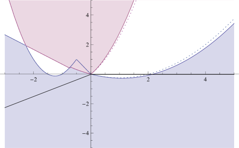
Figure 1: Plot of the exact expressions determined numerically (solid curves) and the approximate analytical expressions in (5.28) and (5.34) (dotted curves) for the upper and lower bounds $m^{2}_{\rm up}$ (blue) and $m^{2}_{\rm low}$ (red) as functions of $\epsilon$. The two shaded areas (blue and red regions) delimit the ranges in which the smallest and the largest mass eigenvalues are allowed to lie. The metastability bound is also shown (solid black lines).

6 Hypers and vectors with several gaugings

Let us finally try to see what happens in the general case of theories with $n_{H}$ hypers and $n_{V}$ vectors with a gauging involving both the vectors and the graviphoton and a generic number $n_{G}$ of isometries. In this general situation, there is no way to avoid the explicit appearance of some indices labeling the gauged isometries. At most, one may switch from the indices $A,B$ running over the $n_{V}+1$ vector fields to new indices $\alpha,\beta$ running only over the $n_{G}$ gauged isometries by first rewriting $k^{u}_{A}=\xi_{A}^{\alpha}k_{\alpha}^{u}$ and $P^{x}_{A}=\xi_{A}^{\alpha}P_{\alpha}^{x}$, and then defining $L^{\alpha}=\xi_{A}^{\alpha}L^{A}$ and $f_{i}^{\alpha}=\xi_{A}^{\alpha}f^{A}_{i}$. The potential then reads

$$V=2\hskip 1.0ptk_{\alpha}^{w}k_{\beta w}L^{\alpha}\bar{L}^{\beta}+\bar{f}^{k\alpha}f_{k}^{\beta}P_{\alpha}^{z}P_{\beta}^{z}-3\hskip 1.0ptP_{\alpha}^{z}P_{\beta}^{z}L^{\alpha}\bar{L}^{\beta}\,,$$ (6.1)

and the stationarity conditions are given by

$$4\hskip 1.0ptk_{\alpha}^{w}\nabla_{u}k_{\beta w}L^{\alpha}\bar{L}^{\beta}+2\hskip 1.0pt\big{(}\bar{f}^{k\alpha}f_{k}^{\beta}-3L^{\alpha}\bar{L}^{\beta}\big{)}P_{(\alpha}^{z}\nabla_{u}P_{\beta)}^{z}=0\,,$$ (6.2)

$$C_{ikl}\bar{f}^{\alpha k}\bar{f}^{\beta l}P_{\alpha}^{z}P_{\beta}^{z}+2\big{(}k_{\alpha}^{w}k_{\beta w}-P_{\alpha}^{z}P_{\beta}^{z}\big{)}f_{i}^{\alpha}\bar{L}^{\beta}=0\,.$$ (6.3)

The relevant blocks of the unnormalized scalar mass matrix are then found to be

$$m^{2}_{uv\!}=-\,4\big{(}R_{urvs}k_{\alpha}^{r}k_{\beta}^{s}-\nabla_{u}k_{\alpha}^{w}\nabla_{v}k_{\beta w}\big{)}L^{\alpha}\bar{L}^{\beta}$$

$$\hskip 35.0pt+\,2\big{(}\bar{f}^{\alpha k}f_{k}^{\beta}-3L^{\alpha}\bar{L}^{\beta}\big{)}\big{(}P_{(\alpha}^{z}\nabla_{u}\nabla_{v}P_{\beta)}^{z}+\nabla_{u}P_{(\alpha}^{z}\nabla_{v}P_{\beta)}^{z}\big{)}\,,$$ (6.4)

$$m^{2}_{\hskip 1.0pti\bar{\jmath}\hskip 1.0pt}=-2\hskip 1.0ptR_{i\bar{\jmath}p\bar{q}}\bar{f}^{\alpha p}f^{\beta\bar{q}}P_{\alpha}^{x}P_{\beta}^{x}+2\hskip 1.0ptf^{\alpha}_{i}\bar{f}^{\beta}_{\bar{\jmath}}k_{\alpha}^{w}k_{\beta w}$$

$$\hskip 35.0pt+\,2\hskip 1.0ptg_{i\bar{\jmath}}L^{\alpha}\bar{L}^{\beta}k_{\alpha}^{w}k_{\beta w}+2\hskip 1.0ptg_{i\bar{\jmath}}\big{(}\bar{f}^{\alpha k}f_{k}^{\beta}-L^{\alpha}\bar{L}^{\beta}\big{)}P_{\alpha}^{z}P_{\beta}^{z}\,,$$ (6.5)

$$m^{2}_{ui}=4\hskip 1.0ptk_{\alpha}^{w}\nabla_{u}k_{\beta w}f_{i}^{\alpha}\bar{L}^{\beta}+2\big{(}C_{ikl}\bar{f}^{\alpha k}\bar{f}^{\beta l}-2\hskip 1.0ptf_{i}^{\alpha}\bar{L}^{\beta}\big{)}P_{(\alpha}^{z}\nabla_{u}P_{\beta)}^{z}\,.$$ (6.6)

The gravitino mass is finally given by

$$m^{2}_{3/2}=P_{\alpha}^{z}P_{\beta}^{z}L^{\alpha}\bar{L}^{\beta}\,.$$ (6.7)

One may now try to look at the mass matrix along some special sets of vectors defining the sGoldstino directions in the hyper and vector sectors. The natural candidates for these are given by the vectors $N_{u}^{x}=|\nabla_{u}P_{\alpha}^{x}L^{\alpha}|$ and $W_{i}^{x}=f_{i}^{\alpha}P_{\alpha}^{x}$ controlling the shifts of the hyperini and the gaugini under supersymmetry transformations. The $3$ vectors $N^{ux}$ are orthogonal and satisfy $g_{uv}N^{ux}N^{vy}=c^{-2}\hskip 1.0pt\delta^{xy}$ with $c=|k_{\alpha}^{w}k_{\beta w}L^{\alpha}\bar{L}^{\beta}|^{-1/2}$. One may then simply rescale the $N^{ux}$ to define $3$ orthonormal vectors $n^{ux}=c\hskip 1.0ptN^{ux}$. The $3$ vectors $W^{ix}$ are not orthogonal and instead satisfy $g_{i\bar{\jmath}}\bar{W}^{ix}W^{\bar{\jmath}y}=d^{xy}$ with $d^{xy}=P^{x}_{\alpha}P^{y}_{\beta}(\bar{f}^{\alpha k}f^{\beta}_{k})$. Moreover, one finds that the $3\times 3$ matrix $d^{xy}$ has rank $r=3$ only if $n_{G}\geq 3$ and $n_{V}\geq 3$. This matrix has rank $2$ when $n_{G}=2$ and $n_{V}\geq 2$, or $n_{G}=3$ and $n_{V}=2$, and rank $1$ when $n_{G}=1$ and $n_{V}\geq 1$ (which includes the case studied in the previous section), or $n_{G}=2$ and $n_{V}=1$. One may then take suitable linear combinations of the $\bar{W}^{ix}$ to define $r$ independent orthonormal vectors $w^{ix^{\prime}}=c^{x^{\prime}}_{x}\bar{W}^{ix}$, with $x^{\prime}=1,..,r$ and $c^{x^{\prime}}_{x}$ such that $c^{x^{\prime}}_{x}\bar{c}^{y^{\prime}}_{y}d^{xy}=\delta^{x^{\prime}y^{\prime}}$. Summarizing, we may thus consider the following two sets of $3$ and $r$ vectors in the two sectors:

$$n^{ux}=c\,|\nabla^{u}P^{x}_{\alpha}L^{\alpha}|=-c\,J^{x}{}^{u}{}_{v}|k_{\alpha}^{v}L^{\alpha}|\,,\;\;w^{ix^{\prime}}=c^{x^{\prime}}_{x}\bar{f}^{\alpha i}P_{\alpha}^{x}\,.$$ (6.8)

These now satisfy $g_{uv}n^{ux}n^{vy}=\delta^{xy}$ and $g_{i\bar{\jmath}}w^{ix^{\prime}}\bar{w}^{\bar{\jmath}y^{\prime}}=\delta^{x^{\prime}y^{\prime}}$. We may then try to proceed as in the previous section and define a $2\times 2$ matrix by averaging over these two special sets of directions within each of the two sectors, with entries given by:

$$m^{2}_{\rm hh}\equiv\text{\small$\frac{1}{3}$}m^{2}_{uv}n^{ux}n^{vx}\,,\;\;m^{2}_{\rm vv}\equiv\text{\small$\frac{1}{r}$}m^{2}_{i\bar{\jmath}}w^{ix^{\prime}\!}\bar{w}^{\bar{\jmath}x^{\prime}\!}\,,$$ (6.9)

$$m^{2}_{\rm hv}\equiv\sqrt{\text{\small$\frac{1}{3\hskip 1.0ptr}$}m^{2}_{ui}n^{ux}w^{ix^{\prime}\!}m^{2}_{v\bar{\jmath}}n^{vx}\bar{w}^{\bar{\jmath}x^{\prime}\!}}\,.$$ (6.10)

However, it turns out that this no longer allows us to eliminate all the dependence on the curvature, and therefore no universal bound emerges in this general case. To see how this comes about, let us focus on the terms in the mass matrix that may a priori depend on $\Sigma_{urvs}$ or $C_{ijk}$, and check whether they still disappear in the same way as before.

In the hyper-hyper block of the averaged scalar mass matrix, one finds that the term involving $R_{usvr}$ gives the following contribution:

$$m^{2}_{uv}n^{ux}n^{vx}\supset-\hskip 1.0pt4\hskip 1.0ptc^{2}R_{urvs}J^{x}{}^{u}{\!}_{p}J^{x}{}^{v}{\!}_{q}k_{\alpha}^{r}k_{\beta}^{s}k_{\gamma}^{p}k_{\delta}^{q}L^{\alpha}\bar{L}^{\beta}L^{\gamma}\bar{L}^{\delta}\,.$$ (6.11)

We now see that the $\Sigma_{urvs}$ part of $R_{urvs}$ also contributes to this contraction, because this now involves the full contraction $R_{urvs}J^{x}{}^{u}{\!}_{p}J^{x}{}^{v}{\!}_{q}$ while only the completely symmetric part of it $R_{(urvs}J^{x}{}^{u}{\!}_{p}J^{x}{}^{v}{\!}_{q)}$ is fixed by the sum rule (2.7). The $\Sigma_{urvs}$ dependence thus disappears only when $n_{G}=1$, or whenever all of the $n_{G}$ sections $L^{\alpha}$ accidentally have the same phase.

In the vector-vector block of the averaged scalar mass matrix, one finds that the term involving $R_{i\bar{\jmath}p\bar{q}}$ gives the following contribution:

$$m^{2}_{i\bar{\jmath}}w^{ix^{\prime}\!}\bar{w}^{\bar{\jmath}x^{\prime}\!}\supset-\hskip 1.0pt2\hskip 1.0ptc^{x^{\prime}}_{x}\!c^{x^{\prime}}_{y}\!R_{i\bar{\jmath}p\bar{q}}\bar{f}^{\alpha i}f^{\beta\bar{\jmath}}\bar{f}^{\gamma p}f^{\delta\bar{q}}P_{\alpha}^{x}P_{\beta}^{y}P_{\gamma}^{z}P_{\delta}^{z}\,.$$ (6.12)

We now see that the $-C_{ipr}g^{r\bar{s}}\bar{C}_{\bar{\jmath}\bar{q}\bar{s}}$ part of $R_{i\bar{\jmath}p\bar{q}}$ also contributes to this contraction, because the $x,y,z$ indices are contracted in a way that no longer allows for any simplification of the result by making use of the stationarity condition (6.3), which fixes the value of $C_{ikl}\bar{f}^{\alpha k}\bar{f}^{\beta l}P_{\alpha}^{z}P_{\beta}^{z}$ and thus of the different contraction $R_{i\bar{\jmath}p\bar{q}}\bar{f}^{\alpha i}f^{\beta\bar{\jmath}}\bar{f}^{\gamma p}f^{\delta\bar{q}}P_{\alpha}^{x}P_{\beta}^{y}P_{\gamma}^{x}P_{\delta}^{y}$. Therefore the $C_{ijk}$ dependence can only be eliminated through the stationarity condition when $n_{V}=1$ and $n_{G}=1,2$, or whenever all of the $n_{G}$ triplets of Killing prepotentials $P^{x}_{\alpha}$ are accidentally parallel.

In the hyper-vector block of the averaged scalar mass matrix, finally, one finds that the term involving $C_{ijk}$ gives the following contribution, after using the equivariance conditions:

$$m^{2}_{ui}n^{ux}w^{ix^{\prime}\!}\!\supset\!c\hskip 1.0ptc^{x^{\prime}}_{y}\!C_{ikl}\bar{f}^{i\alpha}\!\bar{f}^{\beta k}\!\bar{f}^{\gamma l}(2P_{\beta}^{x}P_{\alpha}^{y}k^{w}_{\gamma}k_{\delta w}\!-\!P^{x}_{\gamma}P_{\alpha}^{y}P_{\beta}^{z}P^{z}_{\delta}\!+\!P^{x}_{\delta}P_{\alpha}^{y}P_{\beta}^{z}P^{z}_{\gamma})L^{\delta}\,.$$ (6.13)

We see here too that the $C_{ijk}$ dependence cannot be eliminated from the contraction, because the stationarity condition only fixes the value of $C_{ikl}\bar{f}^{\alpha k}\bar{f}^{\beta l}P_{\alpha}^{z}P_{\beta}^{z}$. The $C_{ijk}$ dependence can again only be eliminated through the stationarity condition when $n_{V}=1$ and $n_{G}=1,2$, or whenever all of the $n_{G}$ triplets of Killing prepotentials $P^{x}_{\alpha}$ are accidentally parallel.

We conclude that whenever $n_{V}\geq 2$ and $n_{G}\geq 2$, and no accidental simplification occurs, there is no way of getting rid of both of the $\Sigma_{urvs}$ and $C_{ijk}$ tensors controlling the curvature of the scalar manifold by averaging over the sGoldstino directions in the two sectors. This implies that no simple universal bound on scalar masses can be derived and strongly suggests that the smallest eigenvalue of the scalar mass matrix can be freely adjusted by tuning the values of the curvature at the stationary point under consideration. To see that this is indeed the case, we can consider tuning the values of $\Sigma_{urvs}$ and $C_{ijk}$, compatibly with the constraints imposed by the stationarity conditions, and then check that all the mass eigenvalues can indeed be made arbitrarily large relative to the gravitino mass. In this respect, we first notice that the values of the independent components of $\Sigma_{urvs}$ are left completely unconstrained by the stationarity conditions in the hyper sector, while the values of the independent components of $C_{ijk}$ are only partly constrained by the stationarity conditions in the vector sector unless additional peculiarities arise. As a result, by taking the values of $\Sigma_{urvs}$ and the unfixed values of $C_{ijk}$ to be large, one may achieve values of ${\cal O}(\Sigma\hskip 1.0ptm^{2}_{3/2})$ for all the entries of $m^{2}_{uv}$ and values of ${\cal O}(|C|^{2}\hskip 1.0ptm^{2}_{3/2})$ for all the entries of $m^{2}_{i\bar{\jmath}}$, while the entries of $m^{2}_{ui}$ will only be of ${\cal O}(C\hskip 1.0ptm^{2}_{3/2})$. After diagonalization, one then finds $4\hskip 1.0ptn_{H}\!-n_{V}$ square mass eigenvalues of ${\cal O}(\Sigma\hskip 1.0ptm^{2}_{3/2})$ and $n_{V}$ square mass eigenvalues of ${\cal O}(|C|^{2}\hskip 1.0ptm^{2}_{3/2})$, since the level repulsion effect induced by the off-diagonal block gives only negligible corrections (of ${\cal O}(m^{2}_{3/2})$ on the former and of ${\cal O}(|C|^{2}\Sigma^{-1}\hskip 1.0ptm^{2}_{3/2})$ on the latter), and all of them are then large with respect to $m^{2}_{3/2}$.

We have performed various checks to verify that there is no general obstruction against achieving the situation described above, where arbitrary values for the scalar masses can be found by adjusting the curvatures of the quaternionic-Kähler and special-Kähler manifolds. It would be very interesting to construct an explicit family of examples where this can be realized concretely. For instance, one could consider the model with one hyper and two gauged isometries which can be described in general by the Calderbank-Pedersen space [26]. Unfortunately, even for this simple case it turns out to be algebraically complex to proceed along the same lines as [16].

Finally, we can also consider the special case with one graviphoton and one vector gauging two isometries (i.e. $n_{G}=2$ and $n_{V}=1$). In this case it is possible to remove the $C_{ijk}$ tensor but not the $\Sigma_{urvs}$ tensor from the scalar mass matrices. This implies that the entries of $m^{2}_{i\bar{\jmath}}$ are fixed, whereas one can still achieve values of ${\cal O}(\Sigma\hskip 1.0ptm^{2}_{3/2})$ for the entries of $m^{2}_{uv}$. One can then see that $\Sigma_{urvs}$ can be tuned to make $4\hskip 1.0ptn_{H}\!-n_{V}$ eigenvalues large, while the smallest of the remaining $n_{V}$ eigenvalues is bounded by $m^{2}_{\rm vv}$. However, it remains unclear whether or not the value of $m^{2}_{vv}$ can be made arbitrarily large by adjusting parameters, i.e. whether or not a bound emerges in this case.

7 Conclusions

In this work, we have studied the question of whether a universal bound exists on the scalar masses in a supersymmetry breaking vacuum of a generic $N=2$ supergravity theory involving both hyper and vector multiplets. We have shown that such a universal bound indeed exists for any theory where at most one isometry is gauged, and depends only on the gravitino mass $m_{3/2}$ and the cosmological constant $V$ at the vacuum. This result generalizes various previous analyses that were carried out for simpler restricted classes of situations involving a minimal type and/or a minimal number of multiplets [1, 2, 16], and implies that in these theories metastable de Sitter vacua can exist for $V\gg m^{2}_{3/2}$, but not for $V\ll m^{2}_{3/2}$. We then argued that such a universal bound does not exist for theories where two or more isometries are gauged, and that in those theories any desired values for the lightest scalar square mass can, in principle, be obtained by suitably adjusting the curvature of the scalar manifold at the vacuum point through the parameters of the model. This implies that in such more general theories metastable de Sitter vacua can exist not only for $V\gg m^{2}_{3/2}$, but also for $V\ll m^{2}_{3/2}$.

We believe that the result presented in this paper represents a useful guideline towards the search for metastable de Sitter vacua or slow-roll inflationary trajectories in supergravity theories emerging from string models, which often have at least some of the characteristics of theories with extended supersymmetry, even if they display only minimal supersymmetry.

Acknowledgements We would like to thank Marta Gomez-Reino and Jan Louis for useful discussions. The research of C. S. and P. S. is supported by the Swiss National Science Foundation (SNSF) under the grant PP00P2-135164, and that of F. C. by the Angelo Della Riccia foundation.

References

- [1] M. Gomez-Reino, J. Louis and C. A. Scrucca, No metastable de Sitter vacua in N=2 supergravity with only hypermultiplets, JHEP 0902 (2009) 003 [arXiv:0812.0884].
- [2] E. Cremmer, C. Kounnas, A. Van Proeyen, J. P. Derendinger, S. Ferrara, B. de Wit and L. Girardello, Vector multiplets coupled to N=2 supergravity: superhiggs effect, flat potentials and geometric structure, Nucl. Phys. B 250 (1985) 385.
- [3] P. Frè, M. Trigiante and A. Van Proeyen, Stable de Sitter vacua from N = 2 supergravity, Class. Quant. Grav. 19 (2002) 4167 [hep-th/0205119].
- [4] J.-C. Jacot and C. A. Scrucca, Metastable supersymmetry breaking in N=2 non-linear sigma-models, Nucl. Phys. B 840 (2010) 67 [arXiv:1005.2523].
- [5] M. Gomez-Reino and C. A. Scrucca, Locally stable non-supersymmetric Minkowski vacua in supergravity, JHEP 0605 (2006) 015 [hep-th/0602246].
- [6] M. Gomez-Reino and C. A. Scrucca, Constraints for the existence of flat and stable non-supersymmetric vacua in supergravity, JHEP 0609 (2006) 008 [hep-th/0606273].
- [7] M. Gomez-Reino and C. A. Scrucca, Metastable supergravity vacua with F and D supersymmetry breaking, JHEP 0708 (2007) 091 [arXiv:0706.2785].
- [8] F. Denef and M. R. Douglas, Distributions of nonsupersymmetric flux vacua, JHEP 0503 (2005) 061 [hep-th/0411183].
- [9] L. Covi, M. Gomez-Reino, C. Gross, J. Louis, G. A. Palma and C. A. Scrucca, De Sitter vacua in no-scale supergravities and Calabi-Yau string models, JHEP 0806 (2008) 057 [arXiv:0804.1073].
- [10] L. Covi, M. Gomez-Reino, C. Gross, J. Louis, G. A. Palma and C. A. Scrucca, Constraints on modular inflation in supergravity and string theory, JHEP 0808 (2008) 055 [arXiv:0805.3290].
- [11] L. Brizi and C. A. Scrucca, The lightest scalar in theories with broken supersymmetry, JHEP 1111 (2011) 013 [arXiv:1107.1596].
- [12] F. Catino, C. A. Scrucca and P. Smyth, Metastable de Sitter vacua in N=2 to N=1 truncated supergravity, JHEP 1210 (2012) 124 [arXiv:1209.0912].
- [13] A. Borghese and D. Roest, Metastable supersymmetry breaking in extended supergravity, JHEP 1105 (2011) 102 [arXiv:1012.3736].
- [14] A. Borghese, R. Linares and D. Roest, Minimal Stability in Maximal Supergravity, [arXiv:1112.3939].
- [15] B. Légeret, C. A. Scrucca and P. Smyth, Metastable spontaneous breaking of N=2 supersymmetry, Phys. Lett. B 722 (2013) 372 [arXiv:1211.7364].
- [16] F. Catino, C. A. Scrucca and P. Smyth, Simple metastable de Sitter vacua in N=2 gauged supergravity, JHEP 1304 (2013) 056 [arXiv:1302.1754].
- [17] L. Alvarez-Gaumé and D. Z. Freedman, Geometrical structure and ultraviolet finiteness in the supersymmetric sigma model, Commun. Math. Phys. 80 (1981) 443.
- [18] L. Alvarez-Gaumé and D. Z. Freedman, Potentials For The Supersymmetric Nonlinear Sigma Model, Commun. Math. Phys. 91 (1983) 87.
- [19] J. Bagger and E. Witten, Matter couplings in N=2 supergravity, Nucl. Phys. B 222 (1983) 1.
- [20] B. de Wit and A. Van Proeyen, Potentials and symmetries of general gauged N=2 supergravity: Yang-Mills models, Nucl. Phys. B 245 (1984) 89.
- [21] B. de Wit, P. G. Lauwers, and A. Van Proeyen, Lagrangians of N=2 supergravity - matter systems, Nucl. Phys. B 255 (1985) 569.
- [22] C. M. Hull, A. Karlhede, U. Lindstrom and M. Rocek, Nonlinear sigma models and their gauging in and out of superspace, Nucl. Phys. B 266 (1986) 1.
- [23] A. Strominger, Special geometry, Commun. Math. Phys. 133 (1990) 163.
- [24] R. D’Auria, S. Ferrara and P. Frè, Special and quaternionic isometries: general couplings in N=2 supergravity and the scalar potential, Nucl. Phys. B 359 (1991) 705.
- [25] L. Andrianopoli, M. Bertolini, A. Ceresole, R. D’Auria, S. Ferrara, P. Fré and T. Magri, N = 2 supergravity and N = 2 super Yang-Mills theory on general scalar manifolds: symplectic covariance, gaugings and the momentum map, J. Geom. Phys. 23 (1997) 111 [hep-th/9605032].
- [26] D. M. J. Calderbank and H. Pedersen, Selfdual Einstein metrics with torus symmetry, J. Diff. Geom. 60 (2002) 485 [math/0105263].