Dynamical quantum repeater using cavity-QED and optical coherent states

Abstract

In the framework of cavity QED, we propose a quantum repeater scheme that uses coherent light and atoms coupled to optical cavities. In contrast to conventional schemes, we exploit solely the cavity QED evolution for the entire quantum repeater scheme and, thus, avoid any explicit execution of quantum logical gates. The entanglement distribution between the repeater nodes is realized with the help of pulses of coherent light interacting with the atom-cavity system in each repeater node. In our previous paper [D. Gonta and P. van Loock, Phys. Rev. A 86, 052312 (2012)], we already proposed a dynamical protocol to purify a bipartite entangled state using the evolution of atomic chains coupled to optical cavities. Here, we incorporate parts of this protocol in our repeater scheme, combining it with dynamical versions of entanglement distribution and swapping.

I Introduction

In classical data transmission, repeaters are used to amplify the data signals (bits) when they become weaker during their propagation through the transmission channel. In contrast to classical information, the above mechanism is impossible to realize when the transmitted data signals are the carriers of quantum information (qubits). In optical systems, for instance, a qubit is typically encoded by means of a single photon which cannot be amplified or cloned without destroying quantum information associated with this qubit nat299 ; pla92 . Therefore, the photon has to propagate along the entire length of the transmission channel which, due to photon loss, leads to an exponentially decreasing probability to receive this photon at the end of the channel.

To avoid exponential decay of a photon wave-packet and preserve its quantum coherence, the quantum repeater was proposed prl81 . This repeater contains three building blocks which have to be applied sequentially. With the help of entanglement distribution, first, a large set of low-fidelity entangled qubit pairs is generated between all repeater nodes. Using entanglement purification, afterwards, high-fidelity entangled pairs are distilled from this large set of low-fidelity entangled pairs by means of local operations performed in each repeater node and classical communication between the nodes prl76 ; prl77 . Entanglement swapping, finally, combines two entangled pairs distributed between the neighboring repeater nodes into one entangled pair, thus, gradually increasing the distance of shared entanglement swap .

Because of the fragile nature of quantum correlations and inevitable photon loss in an optical fiber, in practice, it poses a serious challenge to outperform the direct transmission of photons along the fiber. Up to now, however, only particular building blocks of an optical quantum repeater have been experimentally demonstrated, for instance, bipartite entanglement purification prl90 ; nat443 , entanglement swapping prl96 ; pra71 , and entanglement distribution nat454 ; sc316 between two neighboring nodes. Motivated both by the impressive experimental progress and theoretical advances, various revised and improved implementations of repeaters and their building blocks have been recently proposed pra77 ; pra81 ; pra84a ; rmp83 ; lpr .

Practical and efficient schemes for implementing a quantum repeater are not straightforward. The two mentioned protocols, entanglement purification and entanglement swapping, in general, require feasible and reliable quantum logic, such as single- and two-qubit logical gates. Because of the high complexity and demand of physical resources, entanglement purification is the most challenging part of a quantum repeater. The conventional purification protocols prl77 ; pra59 , for instance, involve multiple applications of controlled-NOT gates which assume sophisticated pulse sequences posing thus a serious bottleneck for most physical realizations of qubits nat443 ; prl104 ; pra71a ; prl85 ; pra78 ; pra67 .

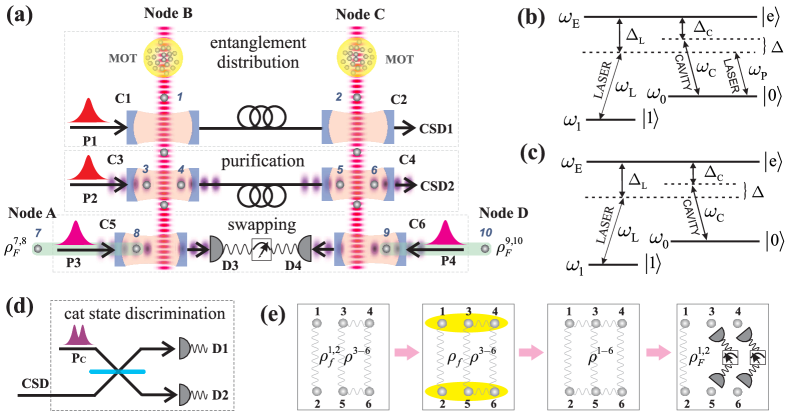
Figure 1: (Color online) (a) Sketch of experimental setup that realizes the two-node repeater scheme. (b, c) Structure of a three-level atom in the $\Lambda$-configuration subjected to the cavity and laser fields. (d) The cat state discrimination (CSD) device. (e) Sequence of steps used in the purification protocol. See text for description.

In our previous papers pra84 ; pra86 , we already suggested a practical scheme to purify dynamically a bipartite entangled state by exploiting solely the evolution of short chains of atoms coupled to high-finesse optical cavities. In the present paper, we make one step further and propose an entire quantum repeater scheme that is realized in the framework of cavity QED and incorporates all three building blocks described above. In contrast to conventional repeater schemes, we exploit solely the cavity QED evolution and, thus, avoid completely quantum logical gates. The entanglement distribution between the repeater nodes is realized with the help of pulses of coherent light interacting sequentially with the atom-cavity systems in each repeater node.

The paper is organized as follows. In the next section, we describe in detail our dynamical quantum repeater scheme. We introduce and discuss the entanglement distribution, purification, and swapping protocols in Secs. II.A, II.B, and II.C, respectively. In Sec. II.D, we discuss a few relevant issues related to the implementation of our repeater scheme, while a brief rate analysis together with a summary and outlook are given in Sec. III.

II Dynamical quantum repeater without quantum gates

The main physical resources of our dynamical repeater are (i) three-level atoms, (ii) high-finesse optical cavities, (iii) continuous and pulsed laser beams, (iv) balanced beam splitters, and (v) photon-number resolving detectors. In Fig. 1(a) we display the sketch of experimental setup that includes two repeater nodes (B and C) and incorporates the entanglement distribution, purification, and swapping protocols in one place.

In this setup, each repeater node includes single-mode cavities $C_{1}$, $C_{3}$, and $C_{5}$ ($C_{2}$, $C_{4}$, and $C_{6}$), a chain of equally distanced atoms conveyed along the setup with the help of an vertical optical lattice, a pair of stationary atoms trapped inside the cavity $C_{3}$ ($C_{4}$) by means of a horizontal optical lattice, source of short coherent-state pulses $P_{3}$ ($P_{4}$), detector $D_{3}$ ($D_{4}$) connected to the neighboring node via a classical communication channel, and a magneto-optical trap (MOT) that plays the role of source for the conveyed atoms. The alignment of vertical lattice is such that the conveyed atoms cross cavities at their anti-nodes ensuring, therefore, a strong atom-cavity coupling once the atom is inside. In addition, the node B contains two coherent-state pulse sources $P_{1}$ and $P_{2}$, while the node C contains two cat state discrimination devices $CSD_{1}$ and $CSD_{2}$. As shown in Fig. 1(d), each such device includes the source $P_{C}$ of single cat states (see below), a balanced beam splitter, and two photon-number resolving detectors $D_{1}$ and $D_{2}$. Both repeater nodes share two chains of atoms ($1$, $2$, and e.t.c.), which are conveyed with a constant velocity through all three cavities, and two pairs of stationary atoms $3$, $4$ and $5$, $6$ trapped inside the cavities $C_{3}$ and $C_{4}$, respectively. The atoms $8$ and $9$ trapped inside the cavities $C_{5}$ and $C_{6}$, respectively, are entangled to the atoms $7$ and $10$ trapped in the repeater nodes A and D.

The setup in Fig. 1(a) is divided in three (framed by dashed rectangles) parts corresponding to the main building blocks of a quantum repeater and mentioned in the introduction. Below, we relate step-by-step our dynamical repeater scheme with this experimental setup and clarify the role of each element.

II.1 Entanglement Distribution

The entanglement distribution protocol is shown in the top rectangle. In this part of setup, the atoms are extracted one-by-one from the MOT, initialized in the ground state $|0\rangle$, and inserted into the conveyor such that the atoms ($1$ and $2$) arrive the cavities $C_{1}$ and $C_{2}$ at the same time. The state $|0\rangle$ together with the state $|1\rangle$ encode a qubit by means of a three-level atom in the $\Lambda$-configuration as displayed in Figs. 1(b) and (c). In order to protect this qubit against the decoherence, the states $|0\rangle$ and $|1\rangle$ are chosen as the stable ground and long-living metastable atomic states or as the two hyperfine levels of the ground state.

Once conveyed into the cavity $C_{1}$ ($C_{2}$), the atom $1$ ($2$) couples simultaneously to the photon field of cavity and two continuous laser beams as displayed in Fig. 1(b). The laser beams act vertically along each conveyor axis and are not depicted in Fig. 1(a) for simplicity. The evolution of coupled atom-cavity-laser system in both repeater nodes is governed by the Hamiltonian

$$H_{ACL}=\frac{\hbar\,J_{1}}{2}\left(a+a^{\dagger}\right)\sigma^{X},$$ (1)

where $\sigma^{X}$ is the respective Pauli operator in the basis $\{|0\rangle,|1\rangle\}$ and $J_{1}$ is the atom-field coupling. We show in Appendix A that the above Hamiltonian is produced deterministically in our setup assuming a strong driving of atom and large atom-field detuning for both laser and cavity fields. Moreover, this Hamiltonian implies that the (fast-decaying) excited state $|e\rangle$ remains almost unpopulated during the evolution. The evolution governed by $H_{ACL}$ yields the operator

$$U_{ACL}(\alpha)=e^{\left(\alpha\,a^{\dagger}-\alpha^{*}a\right)\,\sigma^{X}}=D\left(\alpha\,\sigma^{X}\right)\,,$$ (2)

where $\alpha=-\dot{\iota}\,J_{1}\,t/2$. This operation displaces the cavity field mode by the amount $\alpha$ conditioned on the atomic state. The complex amplitude $\alpha$ is proportional to the atom-cavity-laser evolution time $t$ that, in turn, is inverse proportional to the velocity of conveyed atom.

It has been suggested in Ref. prl101 that the controlled displacement provides an efficient scheme to distribute the entanglement between two atoms coupled to remote cavities. We modify this scheme by considering the feasible atom-cavity-laster evolution (2) controlled by $\sigma^{X}$ and using an input (coherent-state) pulse $\beta$ generated by the source $P_{1}$ that heralds the entanglement distribution. Our modified scheme works as follows. First, the pulse $\beta$ interacts with the atom-cavity-laser system in node B, where the cavity is prepared in the vacuum state, while the atom is initialized in the ground state. Assuming that $\beta^{*}=-\beta$, the evolution (2) leads to the atom-pulse entangled state

$$U^{B}_{ACL}(\alpha)|0_{1}\rangle|\beta\rangle=\frac{1}{\sqrt{2}}\left(|+_{1}\rangle|\beta+\alpha\rangle+|-_{1}\rangle|\beta-\alpha\rangle\right)\,.$$

Once the conveyed atom decouples from the cavity, the pulse in the state $|\beta\pm\alpha\rangle$ leaks out of the cavity and is entirely outputted to the transmission channel between the nodes. Since we are dealing with a high-finesse cavity and since the fast-decaying atomic state $|e\rangle$ remains almost unpopulated during the evolution, the dominant photon loss occurs in the optical fiber that connects the cavities $C_{1}$ and $C_{2}$ and that plays the role of transmission channel in our setup. Apparently, the photon loss increases with the length of the fiber. To a good approximation, therefore, this observation suggests us to describe the loss using the beam splitter model that transmits only a part of the pulse though the channel

$$|\text{vac}\rangle_{E}\,|\beta\pm\alpha\rangle_{F}\longrightarrow|\sqrt{1-\eta}\,(\beta\pm\alpha)\rangle_{E}\,|\tilde{\beta}\pm\tilde{\alpha}\rangle_{F}\,,$$ (3)

where $\tilde{\beta}\pm\tilde{\alpha}=\sqrt{\eta}\,(\beta\pm\alpha)$, while the subscripts $E$ and $F$ refer the environmental and fiber light modes, respectively. Here $\eta=e^{-\ell/\ell_{\circ}}$ describes the attenuation of the transmitted (coherent-state) pulse through the fiber, where $\ell$ is the distance between the repeater nodes, while $\ell_{\circ}$ is the attenuation length that (for fused-silica fibers at telecommunication wavelength) can reach almost $25$ km.

Next, the damped pulse interacts with the atom-cavity-laser system in node C, where (as in the node B) the cavity is prepared in the vacuum state, while the atom is initialized in the ground state. By tracing over the environmental degrees of freedom (modes with the subscript $E$), the evolution $U^{B}_{ACL}(\alpha)$ followed by $U^{C}_{ACL}(\tilde{\alpha})$ leads to the mixed entangled state between the both atoms and the coherent-state pulse

$$\rho=\frac{1+e^{-2|\alpha|^{2}(1-\eta)}}{2}|p\rangle\langle p|+\frac{1-e^{-2|\alpha|^{2}(1-\eta)}}{2}|h\rangle\langle h|\,,$$ (4)

where

$$|p\rangle = \frac{\sqrt{\mathcal{N}_{+}}}{2}|\phi^{+}_{1,2}\rangle|c_{+}\rangle+\frac{\sqrt{\mathcal{N}_{-}}}{2}|\psi^{+}_{1,2}\rangle|c_{-}\rangle+\frac{1}{\sqrt{2}}|\phi^{-}_{1,2}\rangle|\tilde{\beta}\rangle\,;$$

$$|h\rangle = \frac{\sqrt{\mathcal{N}_{-}}}{2}|\phi^{+}_{1,2}\rangle|c_{-}\rangle+\frac{\sqrt{\mathcal{N}_{+}}}{2}|\psi^{+}_{1,2}\rangle|c_{+}\rangle-\frac{1}{\sqrt{2}}|\psi^{-}_{1,2}\rangle|\tilde{\beta}\rangle\,;$$ (5)

$$\quad|c_{\pm}\rangle=\frac{1}{\sqrt{2\,\mathcal{N}_{\pm}}}\left(|\tilde{\beta}+2\,\tilde{\alpha}\rangle\pm|\tilde{\beta}-2\,\tilde{\alpha}\rangle\right)\,,$$

while $\mathcal{N}_{\pm}=1\pm e^{-8\,\eta|\alpha|^{2}}$. The states $|c_{+}\rangle$ and $|c_{-}\rangle$ are the displaced (by the amount $\tilde{\beta}$) even and odd Schrödinger cat states, respectively sch .

The resulting (coherent-state) pulse leaks from $C_{2}$ and is discriminated in the basis $\{|\tilde{\beta}\rangle,|c_{+}\rangle,|c_{-}\rangle\}$ using the cat state discrimination device $CSD_{1}$ (see Sec. II.D). Since $|c_{-}\rangle$ is orthogonal to both $|c_{+}\rangle$ and $|\tilde{\beta}\rangle$, we postselect only the detection events corresponding to this (odd) cat state. With the probability of success $\mathcal{N}_{-}/4$, therefore, the entanglement distribution results into the rank 2 mixed state

$$\rho_{f}^{1,2}=f\,|\psi^{+}_{1,2}\rangle\langle\psi^{+}_{1,2}|+(1-f)|\phi^{+}_{1,2}\rangle\langle\phi^{+}_{1,2}|\,,$$ (6)

where the fidelity of entanglement is given by

$$f=\frac{1}{2}\left(1+\exp{\left[-2|\alpha|^{2}(1-\eta)\right]}\right)\,.$$ (7)

Once the output of measurements corresponds to the state $|\tilde{\beta}\rangle$ or $|c_{+}\rangle$, the entanglement distribution is unsuccessful. In this case, the atoms $1$ and $2$ should be discarded and the entire sequence repeated using the next atomic pair conveyed from MOTs in both repeater nodes. We remark, finally, that the fidelity (7) is close to the unity only when $|\alpha|^{2}(1-\eta)\ll 1$. This observation suggests us to consider the values $|\alpha|\leq 1$ through the paper.

II.2 Entanglement Purification

Assuming that the entanglement distribution is successful, the (low-fidelity) entangled atoms $1$ and $2$ are conveyed along the setup to the purification part displayed in the middle rectangle of Fig. 1(a). In this part of setup, each of cavities $C_{3}$ and $C_{4}$ share a pair of trapped atoms $3$, $4$ and $5$, $6$, respectively. Both cavities are initially prepared in the vacuum state, while the atoms are initialized in the state $|0\rangle$. The entanglement purification is performed in three steps which are displayed in Fig. 1(e) and explained below.

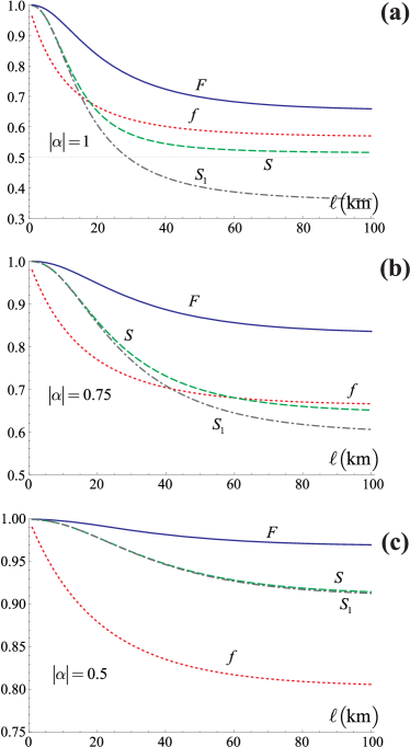
Figure 2: (Color online) For the values (a) $|\alpha|=1$, (b) $|\alpha|=0.75$, and (c) $|\alpha|=0.5$, the solid and dotted curves display the distribution and purification fidelities (7) and (17), respectively. The dot-dashed curves display the swapping fidelity $S_{1}$, while the dashed curves show the fidelity (21) obtained in the conventional swapping protocol.

II.2.1 Four-qubit entanglement generation

Right before atoms $1$ and $2$ are conveyed and coupled to the cavities $C_{3}$ and $C_{4}$, we generate the four-qubit entangled state

$$\rho^{3-6} = \frac{1}{4}\left(1-e^{-8|\alpha|^{2}(1-\eta)}\right)|\phi^{+}_{3,4},\phi^{-}_{5,6}\rangle\langle\phi^{+}_{3,4},\phi^{-}_{5,6}|+\frac{1}{4}\left(1+e^{-8|\alpha|^{2}(1-\eta)}\right)|\psi^{+}_{3,4},\phi^{-}_{5,6}\rangle\langle\psi^{+}_{3,4},\phi^{-}_{5,6}|$$ (8)

$$+ \frac{1}{2}\,e^{-8|\alpha|^{2}(1-\eta)}|\phi^{-}_{3,4},\psi^{+}_{5,6}\rangle\langle\psi^{+}_{3,4},\phi^{-}_{5,6}|+\frac{1}{2}\,e^{-8|\alpha|^{2}(1-\eta)}|\psi^{+}_{3,4},\phi^{-}_{5,6}\rangle\langle\phi^{-}_{3,4},\psi^{+}_{5,6}|+\frac{1}{2}\,|\phi^{-}_{3,4},\psi^{+}_{5,6}\rangle\langle\phi^{-}_{3,4},\psi^{+}_{5,6}|\,,$$

associated with the atoms $3$, $4$, $5$, and $6$. This state is generated using the similar mechanism as utilized in the previous section. Namely, we employ sequentially the evolutions $U_{2ACL}(\alpha)$ and $U_{2ACL}(\tilde{\alpha})$ in repeater nodes B and C, respectively, where $(i=3,4$ or $5,6)$

$$U_{2ACL}(\alpha)=e^{\left(\alpha\,a^{\dagger}-\alpha^{*}a\right)\,\sum\sigma^{X}_{i}}=D\left(\alpha\,\sum\sigma^{X}_{i}\right)\,,$$ (9)

governed by the Hamiltonian

$$H_{2ACL}=\frac{\hbar\,J_{1}}{2}\left(a+a^{\dagger}\right)\sum\sigma^{X}_{i}\,.$$ (10)

This Hamiltonian is produced deterministically in our setup (see Appendix A) and it describes the coupled system of atoms $3$, $4$ ($5$, $6$), photon field of $C_{3}$ ($C_{4}$), and two continuous laser beams which act vertically along each conveyor axis (not depicted in Fig. 1(a) for simplicity).

Similar to the previous section, the pulse $\beta$ (source $P_{2}$) interacts sequentially with the atoms-cavity-laser systems in each repeater node and is discriminated in the basis $\{|\tilde{\beta}\rangle,|c_{+}\rangle,|c_{-}\rangle,|d_{+}\rangle,|d_{-}\rangle\}$ by the $CSD_{2}$ (see Sec. II.D), where

$$|d_{\pm}\rangle=\frac{1}{\sqrt{2\left(1\pm e^{-16\,\eta|\alpha|^{2}}\right)}}\left(|\tilde{\beta}+4\,\tilde{\alpha}\rangle\pm|\tilde{\beta}-4\,\tilde{\alpha}\rangle\right)\,.$$

Only the events corresponding to the output state $|c_{-}\rangle$ are postselected which, with the probability of success $\mathcal{N}_{-}/4$, result into the four-partite entangled state (8).

II.2.2 Evolution for purification

In the previous steps, we have successfully generated the entangled states $\rho_{f}^{1,2}$ and $\rho^{3-6}$ [see the first rectangle of Fig. 1(e)]. In the next step, the atoms $1$ and $2$ are conveyed and coupled to the cavities $C_{3}$ and $C_{4}$, respectively. Since the coherent-state pulse ($P_{2}$) has already left the cavities, they are both in the vacuum state. The conveyed atoms together with the trapped atoms form two atomic triplets $1$, $3$, $4$ and $2$, $5$, $6$. Each of these triplets evolves now due to the periodic Heisenberg XY Hamiltonian ap16 $(i=1,3,4$ or $2,5,6)$

$$H_{XY}=\frac{\hbar\,J_{2}}{2}\sum_{i}\left(\sigma_{i}^{X}\sigma_{i+1}^{X}+\sigma_{i}^{Y}\sigma_{i+1}^{Y}\right),$$ (11)

over the time period $T_{2}=2\,J_{2}^{-1}$, where $\sigma^{X}_{i}$ and $\sigma^{Y}_{i}$ are the Pauli operators and $J_{2}$ is the coupling between the atoms of a given triplet. We show in Appendix B that this Hamiltonian is produced deterministically in our scheme by coupling simultaneously three atoms to the same cavity mode and a laser beam in the limit of large detuning.

The evolution governed by the above Hamiltonian

$$e^{-\frac{\dot{\iota}\,}{\hbar}H_{XY}\,t}=\sum_{j=1}^{8}e^{-\frac{\dot{\iota}\,}{\hbar}E_{j}\,t}\,|\mathbf{k}_{j}\rangle\langle\mathbf{k}_{j}|\,,$$ (12)

is completely determined by the energies $E_{i}$ and vectors $|\mathbf{k}_{i}\rangle$, which satisfy the equality $H_{XY}\,|\mathbf{k}_{i}\rangle=E_{i}\,|\mathbf{k}_{i}\rangle$ along with the orthogonality $\langle\mathbf{k}_{i}|\mathbf{k}_{j}\rangle=\delta_{ij}$ and completeness $\sum|\mathbf{k}_{i}\rangle\langle\mathbf{k}_{i}|=\mathrm{I}$ relations. With the help of Jordan-Wigner transformation zp47 , this eigenvalue problem can be solved exactly (see, for instance, Ref. pra64 ). Since the evolution operator (12) acts on the atomic triplet in node B that is entangled with the atomic triplet in the node C, we consider the evolution operator

$$U_{XY}=\sum_{i,j=1}^{8}e^{-\frac{\dot{\iota}\,}{\hbar}\left(E_{i}+E_{j}\right)\,T_{2}}\,|\mathbf{k}^{B}_{i}\rangle\langle\mathbf{k}^{B}_{i}|\otimes|\mathbf{k}^{C}_{j}\rangle\langle\mathbf{k}^{C}_{j}|\,,$$ (13)

referred to below as the purification and indicated by the ellipses in Fig. 1(e).

According to this evolution, the state of both atomic triplets is described by the six-qubit density operator

$$\rho^{1-6} = U_{XY}\left(\rho_{f}^{1,2}\otimes\rho^{3-6}\right)U^{\dagger}_{XY}$$ (14)

$$= \sum_{i,j=1}^{64}\,\rho^{1-6}_{i,j}\,|\mathbf{v}_{i}\rangle\langle\mathbf{v}_{j}|\,,$$

where $2^{6}$ composite states $|\mathbf{v}_{i}\rangle$, satisfying the orthogonality and completeness relations $\langle\mathbf{v}_{i}|\mathbf{v}_{j}\rangle=\delta_{ij}$ and $\sum|\mathbf{v}_{i}\rangle\langle\mathbf{v}_{i}|=\mathrm{I}$, respectively, have been introduced.

II.2.3 Finalization of the protocol

Once the purification is performed and the conveyed atoms leave the respective cavities, the atoms $3$, $4$ and $5$, $6$ are projected in the computational basis $\{|0\rangle,|1\rangle\}$. Entanglement purification is successful when the outcome of projections coincides with one of combinations

$$\{0_{3},1_{4},0_{5},1_{6}\},\quad\{0_{3},1_{4},1_{5},0_{6}\}\,;$$ (15a)

$$\{1_{3},0_{4},0_{5},1_{6}\},\quad\{1_{3},0_{4},1_{5},0_{6}\}\,.$$ (15b)

With the constant probability of success $1/4$, therefore, the conveyed atoms are described by the density operator

$$\rho^{1,2}_{F} = \frac{1}{\mathcal{N}_{1}}\sum_{\alpha,\beta=1}^{4}\rho^{1-6}_{\alpha,\beta}\,|\mathbf{u}_{\alpha}\rangle\langle\mathbf{u}_{\alpha}|$$ (16)

$$= F\,|\phi^{-}_{1,2}\rangle\langle\phi^{-}_{1,2}|+(1-F)|\psi^{-}_{1,2}\rangle\langle\psi^{-}_{1,2}|\,,$$

where $\mathcal{N}_{1}$ is the respective normalization factor. In this expression, moreover, the purified fidelity is given by

$$F=\frac{\left(0.000548294+0.0016253\,e^{\,8|\alpha|^{2}(1-\eta)}+0.00217359\,e^{\,6|\alpha|^{2}(1-\eta)}\right)f}{0.000538502+0.00163509\,e^{\,8|\alpha|^{2}(1-\eta)}+\left(0.00434718\,f-0.00217359\right)e^{\,6|\alpha|^{2}(1-\eta)}}\,,$$ (17)

while $|\mathbf{u}_{\alpha}\rangle$ are determined by the one of inequalities

$$|\mathbf{u}_{\alpha}\rangle \equiv \langle 0_{3},1_{4},0_{5},1_{6}|\mathbf{v}_{\alpha}\rangle\neq 0\,;$$ (18a)

$$|\mathbf{u}_{\alpha}\rangle \equiv \langle 0_{3},1_{4},1_{5},0_{6}|\mathbf{v}_{\alpha}\rangle\neq 0\,;$$ (18b)

$$|\mathbf{u}_{\alpha}\rangle \equiv \langle 1_{3},0_{4},0_{5},1_{6}|\mathbf{v}_{\alpha}\rangle\neq 0\,;$$ (18c)

$$|\mathbf{u}_{\alpha}\rangle \equiv \langle 1_{3},0_{4},1_{5},0_{6}|\mathbf{v}_{\alpha}\rangle\neq 0\,,$$ (18d)

and correspond to the outcomes of the projections (15).

The operator (16) implies that the entangled state associated with the conveyed atoms $1$ and $2$ preserves its rank 2 form after the purification. Unlike the conventional purification protocol, therefore, the purified state is completely characterized by the fidelity (17). We stress that once the outcome of atomic projections associated with the trapped atoms disagree with (15), the entanglement purification is unsuccessful. In this case, the atoms $1$ and $2$ should be discarded and the entire (repeater) sequence restarted using one fresh atomic pair conveyed from MOTs in each repeater node.

By considering $|\alpha|=1$, $0.75$, and $0.5$, in Fig. 2, we compare the purification fidelity (solid curve) with the fidelity (7) obtained by means of entanglement distribution only (dotted curve). We see that purification yields a significant growth of (input) distribution fidelity. In agreement with Eqs. (7) and (17), moreover, these plots confirm that the smaller values of $|\alpha|$ are chosen, the higher values of both distribution and purification fidelities are obtained. In addition, we infer that both fidelities saturate around $\ell\approx 100$ km and they exhibit an almost constant behavior for $\ell>100$ km.

We remark that the described purification protocol is based on the effect of entanglement transfer between the networks of evolving spin chains that was introduced and investigated in Ref. qip . In the same reference, it was suggested that this effect plays the key role in the entanglement distillation once a part of spins from two such networks are projectively measured. One similar entanglement purification protocol, moreover, has been proposed in Ref. pra78a . In Refs. pra84 ; pra86 , furthermore, we adapted this mechanism to the cavity QED framework, where the role of (spin-chain) networks was played by the atomic triplets coupled to the cavities located in two repeater nodes, while the cavity-mediated interaction (11) reproduced the spin-chain dynamics within a spin network. Using several improvements, in the latter paper, we obtained an almost-unit output fidelity after a few successful purification rounds. In contrast to Ref. pra86 , however, in this paper we consider a notably modified approach to the purification protocol and employ one single purification round.

II.3 Entanglement Swapping

Assuming that both the entanglement distribution and purification were successful, the (high-fidelity) entangled atoms $1$ and $2$ are conveyed along the setup to the swapping part displayed in the bottom rectangle of Fig. 1(a). In this part, the atoms $1$ and $2$ couple the cavities $C_{5}$ and $C_{6}$, both prepared initially in the vacuum state. The conveyed atoms together with the trapped atoms form two atomic pairs $1$, $8$, and $2$, $9$. We recall that atoms $8$ and $9$ are entangled with atoms $7$ and $10$, respectively, where each pair is described by the rank 2 mixed states $\rho^{7,8}_{F}$ and $\rho^{9,10}_{F}$ given both by (16).

Table 1: Bell states corresponding to $\mathbf{s}^{1}_{ij}$ for given $i$ and $j$.

	1	2	3	4
1	$\phi^{-}_{7,10}$	$\phi^{+}_{7,10}$	$\psi^{-}_{7,10}$	$\psi^{+}_{7,10}$
2	$\phi^{+}_{7,10}$	$\phi^{-}_{7,10}$	$\psi^{+}_{7,10}$	$\psi^{-}_{7,10}$
3	$\psi^{-}_{7,10}$	$\psi^{+}_{7,10}$	$\phi^{-}_{7,10}$	$\phi^{+}_{7,10}$
4	$\psi^{+}_{7,10}$	$\psi^{-}_{7,10}$	$\phi^{+}_{7,10}$	$\phi^{-}_{7,10}$

Table 2: Bell states corresponding to $\mathbf{n}^{1}_{ij}$ for given $i$ and $j$.

	1	2	3	4
1	$\phi^{+}_{7,10}$	$\phi^{-}_{7,10}$	$\psi^{-}_{7,10}$	$\psi^{+}_{7,10}$
2	$\phi^{-}_{7,10}$	$\phi^{+}_{7,10}$	$\psi^{+}_{7,10}$	$\psi^{-}_{7,10}$
3	$\psi^{+}_{7,10}$	$\psi^{-}_{7,10}$	$\phi^{-}_{7,10}$	$\phi^{+}_{7,10}$
4	$\psi^{-}_{7,10}$	$\psi^{+}_{7,10}$	$\phi^{+}_{7,10}$	$\phi^{-}_{7,10}$

According to the conventional entanglement swapping protocol swap , the atomic pairs $1$, $8$ and $2$, $9$ are projectively measured in the Bell bases $|\mathbf{b}_{1,8}^{i}\rangle$ and $|\mathbf{b}_{2,9}^{i}\rangle$, respectively, where $(i=1,\ldots,4)$

$$|\mathbf{b}_{a,b}^{i}\rangle=\{|\phi^{+}_{a,b}\rangle,|\phi^{-}_{a,b}\rangle,|\psi^{+}_{a,b}\rangle,|\psi^{-}_{a,b}\rangle\}\,.$$ (19)

This projective measurement results unconditionally into the entangled state between the (initially uncorrelated) atoms $7$ and $10$ increasing, thus, the overall distance of shared entanglement from $\ell$ to $3\,\ell$. In other words, the swapped state is given by the density operator

$$\rho^{7,10}_{S} = \frac{1}{\mathcal{N}_{2}}\langle\mathbf{b}_{1,8}^{i},\mathbf{b}_{2,9}^{j}|\rho^{1,2}_{F}\otimes\rho^{7,8}_{F}\otimes\rho^{9,10}_{F}|\mathbf{b}_{1,8}^{i},\mathbf{b}_{2,9}^{j}\rangle$$ (20)

$$= S\,|\mathbf{s}^{1}_{ij}\rangle\langle\mathbf{s}^{1}_{ij}|+\left(1-S\right)|\mathbf{s}^{2}_{ij}\rangle\langle\mathbf{s}^{2}_{ij}|\,,$$

where $\mathcal{N}_{2}$ is the respective normalization factor. In this expression, moreover, the resulting (swapped) fidelity takes the form

$$S=F(3-6\,F+4\,F^{2})\,,$$ (21)

while $\mathbf{s}^{1}_{ij}$ is displayed in Table 2. Similar to the states $\rho^{7,8}_{F}$, $\rho^{9,10}_{F}$, and $\rho^{1,2}_{F}$, this swapped state $\rho^{7,10}_{S}$ preserves its rank 2 form and is completely characterized by the fidelity (21) displayed in Fig. 2 by dashed curves.

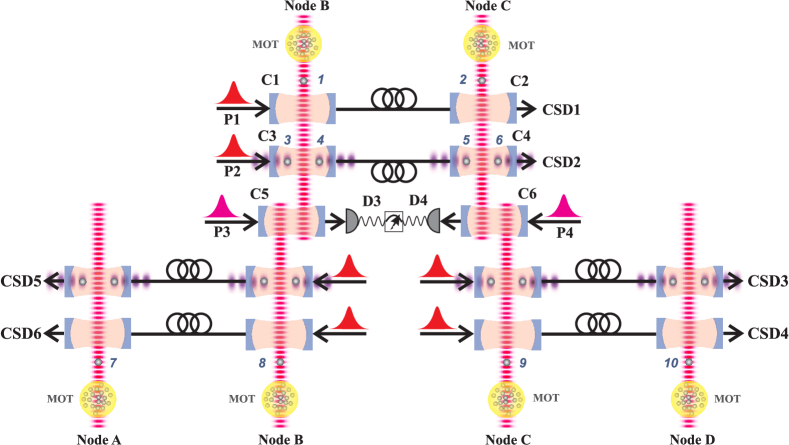
Figure 3: (Color online) Sketch of experimental setup that realizes the four-node repeater scheme.

In our setup, each of atomic pairs evolves in cavity $C_{5}$ or $C_{6}$ due to the periodic Heisenberg XX Hamiltonian $(i=1,8$ or $2,9)$

$$H_{XX}=\frac{\hbar\,J_{2}}{2}\sum_{i}\sigma_{i}^{X}\sigma_{i+1}^{X}\,,$$ (22)

over the time period $T_{3}=\pi\,J_{2}^{-1}/2$. We show in Appendix A that this Hamiltonian is produced deterministically in our setup by coupling simultaneously two atoms to the same cavity mode and laser beams as displayed in Fig. 1(b). The evolution of an atomic pair governed by this Hamiltonian over the period $T_{3}$ implies

$$|1_{a},1_{b}\rangle \longrightarrow \frac{-\dot{\iota}\,}{\sqrt{2}}\left(|0_{a},0_{b}\rangle+\dot{\iota}\,|1_{a},1_{b}\rangle\right)\,;$$ (23a)

$$|0_{a},0_{b}\rangle \longrightarrow \frac{1}{\sqrt{2}}\left(|0_{a},0_{b}\rangle-\dot{\iota}\,|1_{a},1_{b}\rangle\right)\,;$$ (23b)

$$|1_{a},0_{b}\rangle \longrightarrow \frac{-\dot{\iota}\,}{\sqrt{2}}\left(|0_{a},1_{b}\rangle+\dot{\iota}\,|1_{a},0_{b}\rangle\right)\,;$$ (23c)

$$|0_{a},1_{b}\rangle \longrightarrow \frac{1}{\sqrt{2}}\left(|0_{a},1_{b}\rangle-\dot{\iota}\,|1_{a},0_{b}\rangle\right)\,,\quad$$ (23d)

where the resulting states form the modified Bell basis

$$|\mathbf{m}_{a,b}^{i}\rangle=e^{-\frac{\dot{\iota}\,}{\hbar}H_{XX}\,T_{3}}\{|1_{a},1_{b}\rangle,|0_{a},0_{b}\rangle,|1_{a},0_{b}\rangle,|0_{a},1_{b}\rangle\}\,.$$

This evolution suggests an efficient and deterministic realization of entanglement swapping in the framework of cavity QED. Namely, the atomic pairs $1$, $8$ and $2$, $9$ are subjected to the evolution $e^{-\frac{\dot{\iota}\,}{\hbar}H_{XX}\,T_{3}}$ followed by projection in the computational basis $\{|0\rangle,|1\rangle\}$. Obviously, these two steps are equivalent with the projective measurement in the modified Bell basis (23), where the swapped state is given by the expression

$$\rho^{7,10}_{\mathbf{S}} = \frac{1}{\mathcal{N}_{3}}\langle\mathbf{m}_{1,8}^{i},\mathbf{m}_{2,9}^{j}|\rho^{1,2}_{F}\otimes\rho^{7,8}_{F}\otimes\rho^{9,10}_{F}|\mathbf{m}_{1,8}^{i},\mathbf{m}_{2,9}^{j}\rangle$$ (24)

$$= S_{1}\,|\mathbf{n}^{1}_{ij}\rangle\langle\mathbf{n}^{1}_{ij}|+\sum_{k=2}^{4}S_{k}\,|\mathbf{n}^{k}_{ij}\rangle\langle\mathbf{n}^{k}_{ij}|\,,$$

where $\mathcal{N}_{3}$ is the respective normalization factor, $\mathbf{n}^{1}_{ij}$ is displayed in Table 2, while the functions

$$S_{1}=F(1-2\,F+2\,F^{2})\,,\quad S_{2}=2(1-F)F^{2}\,,$$ (25a)

$$S_{3}=1-3\,F+4\,F^{2}-2\,F^{3},\quad S_{4}=2(F-1)^{2}F,\qquad$$ (25b)

fulfill the inequality $S_{1}\gg S_{2}>S_{3}>S_{4}$. The swapped state $\rho^{7,10}_{\mathbf{S}}$ is diagonal in the standard Bell basis (19), where the function $S_{1}$ is identified with the swapping fidelity $F_{\text{final}}$ and displayed in Fig. 2 by dot-dashed curves. We see that for $|\alpha|>0.5$ and $\ell<20$ km, this final fidelity almost coincides with the fidelity (21) obtained by means of conventional swapping protocol (see dashed curve).

The total probability of success associated with the entanglement distribution, purification, and two swappings is given by the expression

$$P_{\text{succ}}=P^{\text{sw}}_{\text{succ}}\,\mathcal{N}^{\,2}_{-}/64=P^{\text{sw}}_{\text{succ}}\left(1-e^{-8|\alpha|^{2}\eta}\right)^{2}/64\,,$$ (26)

where $P^{\text{sw}}_{\text{succ}}$ is the probability of success of two entanglement swappings and is determined mainly by the detection efficiency of atomic projective measurements (see below). For $|\alpha|=0.5$, 0.75, and 1, in Fig. 4, we display the ratio $P_{\text{succ}}/P^{\text{sw}}_{\text{succ}}$ as a function of segment distance $\ell$. It seen that the total probability of success is sensitive to the choice of $|\alpha|$ and it drops dramatically with increasing $\ell$. This plot reveals the trade-off between the length of a repeater segment and the total probability of success.

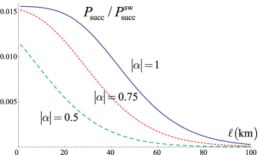
Figure 4: (Color online) The ratio $P_{\text{succ}}/P^{\text{sw}}_{\text{succ}}$ as a function of repeater segment distance $\ell$ for $|\alpha|=1$ (solid line), $|\alpha|=0.75$ (dotted line), and $|\alpha|=0.5$ (dashed line).

II.4 Remarks on the implementation of our scheme

For simplicity, in the setup displayed in Fig. 1(a), we considered just two repeater nodes (B and C), where the atomic pairs $7$, $8$ and $9$, $10$ have been initially entangled and given both by (16). After we explained our repeater scheme, we are ready to introduce the experimental setup that includes explicitly nodes A, B, C, and D. This setup is displayed in Fig. 3 and, in contrast to Fig. 1(a), includes entanglement distribution and purification protocols associated with the atomic pairs $7$, $8$ and $9$, $10$, which are initially disentangled. Simultaneously with the atomic pair $1$, $2$, these pairs are conveyed along the setup (but in the opposite direction) and follow the same sequence of cavity QED evolutions and atomic projective measurements.

We recall that in the framework of entanglement distribution and purifications protocols, the pulses $P_{1}$ and $P_{2}$ are discriminated in the bases $\{|\tilde{\beta}\rangle,|c_{-}\rangle,|c_{+}\rangle\}$ and $\{|\tilde{\beta}\rangle,|c_{-}\rangle,|c_{+}\rangle,|d_{-}\rangle,|d_{+}\rangle\}$ once they leave the cavities $C_{2}$ and $C_{4}$, respectively. In our setup, this discrimination is performed using the cat state discrimination devices $CSD_{1}$ and $CSD_{2}$. As shown in Fig. 1(d), each such device includes a source $P_{C}$ of single cat states $|c_{\pm}\rangle$, a balanced beam splitter, and two photon-number resolving detectors $D_{1}$ and $D_{2}$.

We recall the property of cat states to interfere on a balanced beam splitter by producing an (amplitude) amplified cat state in one output mode and no photons in another output mode pra70 . This property suggest the following discrimination procedure. Once the leaked pulse leaves the respective cavity, it interferes on the beam splitter with $|c_{+}\rangle$ or $|c_{-}\rangle$ generated by $P_{C}$. If both detectors $D_{1}$ and $D_{2}$ produce clicks, then the leaked pulse is either $|\tilde{\beta}\rangle$ or $|d_{\pm}\rangle$. However, if one of detectors produces no clicks, then the state (leaving the other mode of beam splitter) is either an even or odd (amplified) cat state. In contrast to an even cat state, the odd cat state contains an odd number of photons on the top of $|\sqrt{2}\,\tilde{\beta}|^{2}$. This feature plays a decisive role in the discrimination between these cat states by means of the photon-number resolving detector. We remark, finally, that the generation of $|c_{\pm}\rangle$ by the source $P_{C}$ can be deterministically realized using the cavity QED evolution $U_{ACL}(2\,\tilde{\alpha})$ [see (2)] with an input pulse $|\tilde{\beta}\rangle$, such that $\tilde{\beta}^{*}=-\tilde{\beta}$. Assuming that the atom was initialized in the ground state $|0\rangle$ and the cavity in the vacuum state, this evolution results into the states $|c_{+}\rangle$ or $|c_{-}\rangle$ conditioned upon the detection of atom in the state $|0\rangle$ or $|1\rangle$, respectively.

We recall that all three building blocks of our repeater require an efficient technique for projective measurements of atoms which are trapped in (or conveyed through) a cavity. The method of atomic non-destructive measurements demonstrated in Refs. prl97 ; prl103 enables projective measurements of single atoms coupled (strongly) to a cavity field and fits perfectly in our experimental setup. The physical mechanism behind these measurements exploits the suppression of cavity transmission that arises due to the strong atom-cavity coupling. Recall that each atom in our scheme is a three-level atom in the $\Lambda$-configuration [see Figs. 1(b) and (c)], where only the states $|0\rangle$ and $|e\rangle$ are coupled to the cavity field. If one such atom couples the cavity and is prepared in the $|0\rangle$ state, such that the cavity resonance is sufficiently detuned from the atomic $|0\rangle\leftrightarrow|e\rangle$ transition frequency, then the cavity transmission drops according to the atom-cavity detuning and atom-cavity coupling. On the other hand, the cavity transmission remains unaffected if the atom was prepared in the state $|1\rangle$.

Once sufficiently many readouts of the cavity transmission are recorded, the mechanism described above enable us to determine the state of a single atom with a reasonably high efficiency prl97 . Since the atom-cavity coupling increases proportionally with the number of loaded atoms, the same mechanism enables us to distinguish the following three composite states of two trapped atoms (i) $|0_{a},0_{b}\rangle$, (ii) $|0_{a},1_{b}\rangle$ or $|1_{a},0_{b}\rangle$, and (iii) $|1_{a},1_{b}\rangle$ (see prl103 ). We remark, however, that this technique cannot distinguish between the states $|0_{a},1_{b}\rangle$ and $|1_{a},0_{b}\rangle$ leading to an incomplete knowledge about the swapped state (24) [see Table 2]. In order to avoid this drawback, one of the atoms in $C_{5}$ ($C_{6}$) should decouple the cavity right after the indecisive detection occurs and the entire measurement sequence should be repeated with a single atom in the cavity. The decoupling of an atom from the cavity, for instance, can be realized by conveying one from the atoms further along the setup.

In addition, the projective measurements of atomic pairs $3$, $4$ and $5$, $6$ in cavities $C_{3}$ and $C_{4}$ are realized using a probe beam (tuned to the cavity resonance frequency) produced by the source $P_{2}$ and one of the photon detectors in $CSD_{2}$ that monitors the transmission on the other end-point of the fiber. During these projective measurements, the cat state source $P_{C}$ in the upper input mode of beams splitter is switched off. In this case, the probe beam includes the contributions from transmission of both cavities. Recall that a successful purification event is conditioned upon the combinations (15) of atomic projective measurements. These combinations imply that only one atom in each cavity is excited. However, the combinations $\{0_{3},0_{4},1_{5},1_{6}\}$ and $\{1_{3},1_{4},0_{5},0_{6}\}$ lead to the same output of signal transmission and have to be distinguished from the combinations (15). In order to discriminate this outcome that implies a successful purification, the transmission characteristics (i.e., the atom-cavity detuning and coupling) associated with $C_{3}$ and $C_{4}$ should reasonably deviate.

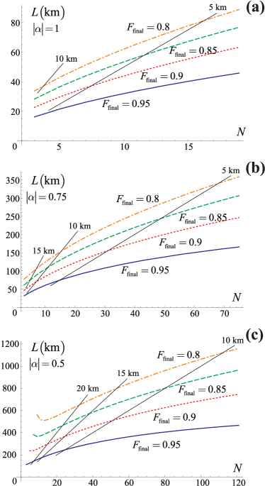
Figure 5: (Color online) For the values (a) $|\alpha|=1$, (b) $|\alpha|=0.75$, and (c) $|\alpha|=0.5$, we display the overall repeater length $L\equiv N\ell$ as a function of number of segments $N$ plotted for the final fidelities $F_{\text{final}}=0.95$ (thick solid curve), $F_{\text{final}}=0.9$ (dotted curve), $F_{\text{final}}=0.85$ (dashed curve), and $F_{\text{final}}=0.8$ (dot-dashed curve). The thin solid lines reveal the maximally achievable length of repeater for a given final fidelity corresponding to a constant segment distance of $5$ km, $10$ km, $15$ km, or $20$ km. See text for details.

Finally, the approach presented in this section requires that atoms are transported with a constant velocity along the experimental setup and coupled to the cavity and laser fields in a controllable fashion. For this purpose, we introduced in our setup magneto-optical traps (MOTs) which play the role of atomic source and optical lattices (conveyors) which transport atoms with a position and velocity control over the atomic motion. The proposed setup is compatible with the existing experimental setups prl95 ; prl98 ; njp10 , in which both MOTs and conveyors are integrated into the same experimental framework with a high-finesse optical cavity. The number-locked insertion technique njp12 , moreover, enables one to extract atoms from MOT and insert a predefined pattern of them into an optical lattice with a single-site precision. By encoding a qubit with the help of hyperfine atomic levels, finally, it has been demonstrated that an optical lattice preserves the coherence of this qubit over seconds prl91 ; prl93 .

III Summary and Outlook

Table 3: Various repeater characteristics for $|\alpha|=1$.

$F_{\text{final}}$	$\ell$	$N$	$R$	$L$
0.95	5.4 km	3	39 pps	16.3 km
0.9	5.1 km	7	25 pps	36 km
0.85	5.1 km	11	19.2 pps	56.4 km
0.8	5.2 km	15	15.8 pps	77.7 km

Table 4: Various repeater characteristics for $|\alpha|=0.75$.

$F_{\text{final}}$	$\ell$	$N$	$R$	$L$
0.95	5 km	15	15.7 pps	74.8 km
0.9	5 km	31	10.2 pps	155.2 km
0.85	5 km	47	7.9 pps	239 km
0.8	5 km	67	6.5 pps	337.6 km
0.95	10.6 km	3	17.9 pps	31.8 km
0.9	10 km	7	11.6 pps	70 km
0.85	10 km	11	8.9 pps	110 km
0.8	10.1 km	15	7.4 pps	151.8 km

Table 5: Various repeater characteristics for $|\alpha|=0.5$.

$F_{\text{final}}$	$\ell$	$N$	$R$	$L$
0.95	10 km	25	3.4 pps	247.5 km
0.9	10 km	51	2.2 pps	510.7 km
0.85	10 km	79	1.7 pps	796 km
0.8	10 km	111	1.4 pps	1115.3 km
0.95	15.5 km	11	2.7 pps	170.8 km
0.9	15.5 km	23	1.8 pps	356.4 km
0.85	15.3 km	37	1.4 pps	565 km
0.8	15 km	53	1.2 pps	798 km
0.95	20.2 km	7	2.2 pps	141.7 km
0.9	20 km	15	1.5 pps	298.4 km
0.85	20.2 km	23	1.1 pps	463.7 km
0.8	20.6 km	31	0.9 pps	639.1 km

In the previous sections, we introduced our repeater scheme with three segments (four nodes) corresponding to the overall distance $3\,\ell$. The final fidelity $F_{\text{final}}$ was identified with the swapping fidelity $S_{1}$ [see (25a)], while the total probability of success was given by (26). The probability of success $P^{\text{sw}}_{\text{succ}}$ associated with this entanglement swapping is determined mainly by the detection efficiency of atomic projective measurements prl97 .

The extension to an arbitrary amount of segments $N$ of the (three-segment) repeater shown in Fig. 3 is straightforward. For convenience, we consider odd values of $N$ corresponding to $N+1$ repeater nodes (or $N-1$ swapping operations). For $|\alpha|=1$, $0.75$, and $0.5$, we display in Fig. 5 the dependence of the overall distance on the amount of repeater segments taken for the final fidelities $F_{\text{final}}=0.8$, $0.85$, $0.9$, and $0.95$. The thin solid lines reveal the maximally achievable overall distances along with the required amount of swappings corresponding to the segment distances $\ell=5$ km and $10$ km [in Fig. 5(a)] or $\ell=10$ km, $15$ km, and $20$ km [in Figs. 5(b) and (c)]. As expected, in all three figures the segment length $\ell$ decreases with the growing of $N$. This happens due to the lack of (re)purification mechanism in our scheme that has to act each time after the execution of several swappings.

Since small segment lengths lead to a rather dense distribution of repeater nodes implying unreasonably high demand of physical resources and since large segment lengths imply small probabilities of success (see Fig. 4), we intentionally bounded $N$ by the range $5$ km $\leq\ell\leq 10$ km for $|\alpha|=1$ and $10$ km $\leq\ell\leq 20$ km for $|\alpha|=0.75$ and $|\alpha|=0.5$. We observe, furthermore, that small values of $|\alpha|$ along with small values of final fidelities $F_{\text{final}}$ lead both to high overall distances $L\equiv N\ell$ of repeater. For $|\alpha|=0.5$ and $\ell=10$ km, for instance, our repeater distributes one entangled pair over the distance of almost $1115$ km with $F_{\text{final}}=0.8$ and $P_{\text{succ}}/P^{\text{sw}}_{\text{succ}}\approx 0.0085$. For $|\alpha|=1$, the same segment length, and the same final fidelity, in contrast, the entanglement is distributed over the distance of almost $34$ km with $P_{\text{succ}}/P^{\text{sw}}_{\text{succ}}\approx 0.015$.

Besides the analysis of the final fidelities and probabilities of success, we compute the repeater rates which provide together the main characteristics of a quantum repeater. Since the atomic (fast-decaying) excited state remains unpopulated and the qubit is encoded by means of long-living atomic states, we assume that the coherence of atoms and cavities exceeds the overall time required to complete the entanglement distribution, purification, and swapping protocols in all repeater nodes. This assumption corresponds to a repeater with ideal memory and implies that the main source of decoherence is the photon loss in the optical fiber pra83 . Since the probability of success is rather small in our scheme (see Fig. 4), we compute the repeater rates (in units of pairs per second) using the expression rmp83

$$R=\left(\frac{2}{3}\right)^{n}\frac{P_{\text{succ}}}{T_{\circ}}\,,$$ (27)

where $T_{\circ}$ is the time required to distribute and purify an entangled state over a single repeater segment being followed by two swappings, $P_{\text{succ}}$ is the probability of success (26), while $n$ is given by the equality $2^{\,n}=N$.

Since the cavity based atomic measurements operate with a high efficiency prl97 , to a good approximation, we set $P^{\text{sw}}_{\text{succ}}=0.9$. In accordance with the experimental setup shown in Fig. 1(a), moreover, we set $T_{\circ}=7\,\ell/\tilde{c}$, where $\tilde{c}=2\cdot 10^{8}$ m$/$s is the speed of light in the optical fiber. The rate (27) is determined by the triplet $\{|\alpha|,\ell,N\}$ that we extract from Fig. 5 for a given value of the final fidelity $F_{\text{final}}$. For instance, for $L=33$ km, $|\alpha|=1$, and $F_{\text{final}}=0.8$, we find that $\ell=11$ km, $N=3$, and $P_{\text{succ}}=0.014$. Being inserted in Eq. (27), these values imply $R\approx 18$ pairs per second (pps). In a similar fashion, we display in Tables 5, 5, and 5 the rates calculated for various values of $\ell$, $F_{\text{final}}$, and $|\alpha|$.

In this paper, a fully cavity QED-based quantum repeater including entanglement distribution, purification, and swapping protocols was proposed. In contrast to conventional repeater schemes, we completely avoid the explicit use of quantum logical gates by exploiting solely cavity QED evolution. Our repeater scheme has a conveyor structure design, in which a chain of initialized single atoms is inserted into an optical lattice and conveyed along the entire repeater node. At the same time, another chain of initialized atoms is conveyed along the neighboring repeater node in a synchronous fashion. These two nodes form together a repeater segment, while the entire set of segments form the quantum repeater itself. Each atomic chain is conveyed through the entanglement distribution and purification blocks, such that each synchronized atomic pair becomes entangled and (afterwards) purified in a probabilistic fashion. Finally, the purified atomic pair is conveyed into the entanglement swapping block, where two entangled atomic pairs distributed between the neighboring repeater nodes are deterministically combined into one entangled pair distributed over a longer distance.

A detailed experimental setup was proposed in Figs. 1(a), 3 and a complete description of all necessary steps and manipulations was provided. A comprehensive analysis of the final fidelities obtained after multiple swapping operations was performed and the correlation between the overall and the segment distances was determined by means of Fig. 5. Moreover, a rate analysis has been performed and the main repeater characteristics have been revealed in Tables 5, 5, and 5. Following recent developments in cavity QED, moreover, we briefly pointed to and discussed a few practical issues related to the implementation of our purification scheme, including the main limitation that arises due to the lack of (re)purification mechanism. We stress that although the proposed quantum repeater is experimentally feasible, its explicit realization for a long-distance quantum communication still poses a serious challenge.

Finally, we like to mention Ref. prl101 by Munro and co-authors in which an entanglement distribution scheme was proposed. In contrast to our approach based on the displacement operator (2) and controlled by $\sigma^{X}$, the approach of Munro and co-authors is based on the displacement controlled by $\sigma^{Z}$ which appears less feasible in the framework of cavity QED. A practical consequence of using the $\sigma^{X}$ displacement instead of $\sigma^{Z}$ is that the remote atoms have to be initialized in the ground state and not in an equal superposition of both basis states as in the approach of Munro and co-authors. In our scheme, moreover, we used an input (coherent-state) pulse $\beta$ generated by the source $P_{1}$ that heralds the generation of state (4).

Appendix A Derivation of the Hamiltonians
(1), (10), and (22)

In this appendix, we show that the Hamiltonians (1), (10), and (22) are produced deterministically in our setup. Specifically, $N$ (three-level) atoms are subjected simultaneously to the field of (initially empty) cavity and fields of two laser beams as displayed in Fig. 1(b). The evolution of this coupled atoms-cavity-laser system is governed by the Hamiltonian ($k=1,2,\ldots,N$)

$$H_{1} = \hbar\,\omega_{C}\,a^{\dagger}\,a-\dot{\iota}\,\hbar\sum_{k}\left[\frac{g}{2}\,a\,|e\rangle_{k}\langle 0|\right.$$

$$+ \left.\frac{\Omega}{2}\left(e^{-i\omega_{L}\,t}|e\rangle_{k}\langle 1|+e^{-i\omega_{P}\,t}|e\rangle_{k}\langle 0|\right)-H.c.\right]$$

$$+ \hbar\sum_{k}\left[\omega_{1}|1\rangle_{k}\langle 1|+\omega_{E}|e\rangle_{k}\langle e|+\omega_{0}|0\rangle_{k}\langle 0|\right]\,,$$

where $g$ denotes the coupling strength of atoms to the cavity mode, while $\Omega$ denotes the coupling strengths of atoms to both laser fields.

We switch to the interaction picture using the unitary transformation

$$U_{1}=e^{-\dot{\iota}\,t\left[\sum\left(\omega_{1}|1\rangle_{k}\langle 1|+\left(\widetilde{\omega}+\Delta_{L}\right)|e\rangle_{k}\langle e|+\omega_{0}|0\rangle_{k}\langle 0|\right)+\left(\widetilde{\omega}-\omega_{0}\right)\,a^{\dagger}a\right]}.$$

where $\widetilde{\omega}\equiv\omega_{1}+\omega_{L}$. In this picture, the Hamiltonian (A) takes the form

$$H_{2} = \hbar\,\Delta\,a^{\dagger}a-\dot{\iota}\,\hbar\sum_{k}\left[\frac{g}{2}\,e^{-i\Delta_{L}\,t}a\,|e\rangle_{k}\langle 0|\right.$$ (29)

$$+ \left.\frac{\Omega}{2}\,e^{-i\Delta_{L}\,t}\left(|e\rangle_{k}\langle 1|+|e\rangle_{k}\langle 0|\right)-H.c.\right].$$

where the notation $\Delta_{L}\equiv(\omega_{E}-\omega_{1})-\omega_{L}$, $\Delta_{C}\equiv(\omega_{E}-\omega_{0})-\omega_{C}$, and $\Delta\equiv\Delta_{L}-\Delta_{C}$ has been introduced.

We require that $\Delta_{L}$ and $\Delta_{C}$ are sufficiently far detuned, such that no atomic $|e\rangle\leftrightarrow|0\rangle$ or $|e\rangle\leftrightarrow|1\rangle$ transitions can occur. We expand the evolution governed by the Hamiltonian (29) in series and keep the terms up to the second order,

$$U_{2}\cong\mathrm{I}-\frac{\dot{\iota}\,}{\hbar}\int_{0}^{t}H_{2}\,dt^{\prime}-\frac{1}{\hbar^{2}}\int_{0}^{t}\left(H_{2}\,\int_{0}^{t^{\prime}}H_{2}\,dt^{\prime\prime}\right)dt^{\prime}\,.$$

By performing integration and retaining only linear-in-time contributions, we express this evolution in the form

$$U_{2}\cong\mathrm{I}-\frac{\dot{\iota}\,}{\hbar}\,H_{3}\,t\cong\exp\left[-\frac{\dot{\iota}\,}{\hbar}\,H_{3}\,t\right],$$ (30)

where the effective Hamiltonian is given by

$$H_{3}=\hbar\,\Delta\,a^{\dagger}a+\frac{\hbar\,\Omega}{4\Delta_{L}}\sum_{k}\left[\Omega\,|1\rangle_{k}\langle 0|+g\,|1\rangle_{k}\langle 0|\,a+H.c.\right]$$

after removing constant contributions. We switch to the interaction picture with respect to the first term of $H_{3}$. In this picture, we obtain

$$H_{4}=\frac{\hbar\,\Omega}{4\Delta_{L}}\sum_{k}\left[\Omega\,|1\rangle_{k}\langle 0|+g\,e^{-i\Delta\,t}|1\rangle_{k}\langle 0|\,a+H.c.\right]\,.$$ (31)

We switch now from the atomic basis $\{|0\rangle,|1\rangle\}$ to the basis $\{|+\rangle,|-\rangle\}$, where

$$|+\rangle=\frac{1}{\sqrt{2}}\left(|0\rangle+|1\rangle\right);\quad|-\rangle=\frac{1}{\sqrt{2}}\left(|0\rangle-|1\rangle\right).$$ (32)

In this basis, the Hamiltonian (31) takes the form

$$H_{5} = \frac{\hbar\,\Omega}{8\Delta_{L}}\sum_{k}\left[2\,\Omega S^{Z}_{k}+g\left(S^{Z}_{k}(e^{-i\Delta\,t}a+e^{i\Delta\,t}a^{\dagger})\right.\right.$$ (33)

$$\hskip 42.67912pt\left.\left.+(S^{\dagger}_{k}-S_{k})(e^{-i\Delta\,t}a-e^{i\Delta\,t}a^{\dagger})\right)\right],\qquad$$

where $S_{k}\equiv|-\rangle_{k}\langle+|$ and $S^{Z}_{k}\equiv|+\rangle_{k}\langle+|-|-\rangle_{k}\langle-|$, and where we removed all the constant contributions. We switch again to the interaction picture with respect to the first term of (33). In this picture, we obtain

$$H_{6} = \hbar\,\frac{g\,\Omega}{8\Delta_{L}}\sum_{k}\left[S^{Z}_{k}(e^{-i\Delta\,t}a+e^{i\Delta\,t}a^{\dagger})\right.$$

$$\left.+(S^{\dagger}_{k}\,e^{\dot{\iota}\,\frac{\Omega^{2}}{2\Delta_{L}}t}-S_{k}\,e^{-\dot{\iota}\,\frac{\Omega^{2}}{2\Delta_{L}}t})(e^{-i\Delta\,t}a-e^{i\Delta\,t}a^{\dagger})\right].$$

In the strong driving regime, i.e., for $\Omega^{2}/(2\,\Delta_{L})\gg\{\Delta,\,g\,\Omega/(8\Delta_{L})\}$, we eliminate the last (fast oscillating) term using the same arguments as for the rotating wave approximation. Using the identity $S^{Z}_{k}=\sigma^{X}_{k}$, the Hamiltonian (A) reduces to

$$H_{7}=\hbar\,\frac{g\,\Omega}{8\Delta_{L}}\left(e^{-i\Delta\,t}a+e^{i\Delta\,t}a^{\dagger}\right)\sum_{k}\sigma^{X}_{k}\,.$$ (35)

In the case of vanishing $\Delta$ (equivalently $\Delta_{L}=\Delta_{C}$), the above Hamiltonian takes the simplified form

$$H_{8}=\hbar\,\frac{g\,\Omega}{8\Delta_{L}}\left(a+a^{\dagger}\right)\sum_{k}\sigma^{X}_{k}\,,$$ (36)

which, under the notation $J_{1}\equiv g\,\Omega/(4\,\Delta_{L})$, coincides with the Hamiltonian (1) for $N=1$ and with the Hamiltonian (10) for $N=2$.

In the case $\Delta_{L}\neq\Delta_{C}$, furthermore, we require that $\Delta$ is sufficiently far detuned and expand the evolution governed by (35) in series up to the second order. By performing integration and retaining only linear-in-time contributions, we express this evolution in the form (30), where the resulting (effective) Hamiltonian

$$H_{9}=\frac{\hbar\,g^{2}\Omega^{2}}{64\,\Delta_{L}^{2}\,\Delta}\sum_{i,j}^{i\neq j}\left[\sigma_{i}^{\dagger}\sigma_{j}^{\dagger}+\sigma_{i}^{\dagger}\sigma_{j}+\sigma_{i}\,\sigma_{j}^{\dagger}+\sigma_{i}\,\sigma_{j}\right]$$ (37)

coincides with the Hamiltonian (22) under the notation $J_{2}\equiv g^{2}\Omega^{2}/(16\,\Delta_{L}^{2}\,\Delta)$, where $\sigma_{i}\equiv|0\rangle_{k}\langle 1|$.

Appendix B Derivation of the Hamiltonian (11)

In this appendix, we show that the Hamiltonian (11) is produced deterministically in our setup. Specifically, three (three-level) atoms are subjected simultaneously to the field of (initially empty) cavity and field of a laser beam as displayed in Fig. 1(c). The evolution of this coupled atoms-cavity-laser system is governed by the Hamiltonian ($k=1,2,3$)

$$H_{10} = \hbar\,\omega_{C}\,a^{\dagger}\,a$$

$$- \dot{\iota}\,\hbar\sum_{k}\left[\frac{g}{2}\,a\,|e\rangle_{k}\langle 0|+\frac{\Omega}{2}\,e^{-i\omega_{L}\,t}|e\rangle_{k}\langle 1|-H.c.\right]$$

$$+ \hbar\sum_{k}\left[\omega_{1}|1\rangle_{k}\langle 1|+\omega_{E}|e\rangle_{k}\langle e|+\omega_{0}|0\rangle_{k}\langle 0|\right]\,,$$

where $g$ denotes the coupling strength of atoms to the cavity mode, while $\Omega$ denotes the coupling strength of atoms to the laser field.

We switch to the interaction picture using the unitary transformation

$$U_{3}=e^{-\dot{\iota}\,t\left[\sum\left(\omega_{1}|1\rangle_{k}\langle 1|+\omega_{E}|e\rangle_{k}\langle e|+\omega_{0}|0\rangle_{k}\langle 0|\right)+\left(\omega_{1}+\omega_{L}-\omega_{0}\right)a^{\dagger}a\right]}.$$

In this picture, the Hamiltonian (B) takes the form

$$H_{11} = \hbar\,\Delta\,a^{\dagger}\,a$$

$$- \dot{\iota}\,\hbar\sum_{k}\left[\frac{g}{2}\,a\,e^{i\Delta_{L}\,t}|e\rangle_{k}\langle 0|+\frac{\Omega}{2}\,e^{i\Delta_{L}\,t}|e\rangle_{k}\langle 1|-H.c.\right],$$

where the notation $\Delta_{L}\equiv(\omega_{E}-\omega_{1})-\omega_{L}$, $\Delta_{C}\equiv(\omega_{E}-\omega_{0})-\omega_{C}$, and $\Delta\equiv\Delta_{L}-\Delta_{C}$ has been introduced.

We require that $\Delta_{L}$ and $\Delta_{C}$ are sufficiently far detuned, such that no atomic $|e\rangle\leftrightarrow|0\rangle$ and $|e\rangle\leftrightarrow|1\rangle$ transitions can occur. We expand the evolution governed by the Hamiltonian (B) in series up to the second order. By performing integration and retaining only linear-in-time contributions, we express this evolution in the form (30), where the effective Hamiltonian is given by (we assume that the cavity field is initially in the vacuum state)

$$H_{12}=\hbar\,\Delta\,a^{\dagger}\,a+\hbar\,\frac{g\,\Omega}{4\,\Delta_{L}}\sum_{k}\left[a\,|1\rangle_{k}\langle 0|+H.c.\right]\,.$$ (40)

We switch one more time to the interaction picture with respect to the first term of (40). In this interaction picture, the resulting Hamiltonian takes the form

$$H_{13}=\hbar\,\frac{g\,\Omega}{4\,\Delta_{L}}\sum_{k}\left[a\,e^{-i\Delta\,t}|1\rangle_{k}\langle 0|+H.c.\right]\,.$$ (41)

We require, finally, that $\Delta$ is sufficiently far detuned. As above, we expand again the evolution governed by the Hamiltonian (41) in series up to the second order and retain only linear-in-time contributions after the integration. This leads to the effective Hamiltonian

$$H_{14}=\frac{\hbar\,g^{2}\Omega^{2}}{16\,\Delta_{L}^{2}\,\Delta}\left[\sum_{i,j}^{i\neq j}|0_{i},1_{j}\rangle\langle 1_{i},0_{j}|+\sum_{k}|1\rangle_{k}\langle 1|\right]\,.$$ (42)

Since the second term in this Hamiltonian commutes with the first term, we eliminate the second term by means of an appropriate interaction picture. The resulting Hamiltonian, i.e., the first term of (42), coincides with the Hamiltonian (11) under the notation $J_{2}\equiv g^{2}\Omega^{2}/(16\,\Delta_{L}^{2}\,\Delta)$.

References

- (1) W. K. Wootters and W. H. Zurek, Nature 299, 802 (1982).
- (2) D. Dieks, Phys. Lett. A 92A, 271 (1982).
- (3) H.-J. Briegel, W. Dür, J. I. Cirac, and P. Zoller, Phys. Rev. Lett. 81, 5932 (1998).
- (4) C. H. Bennett, G. Brassard, S. Popescu, B. Schumacher, J. A. Smolin, and W. K. Wootters, Phys. Rev. Lett. 76, 722 (1996).
- (5) D. Deutsch, A. Ekert, R. Jozsa, C. Macchiavello, S. Popescu, and A. Sanpera, Phys. Rev. Lett. 77, 2818 (1996).
- (6) M. Zukowski, A. Zeilinger, M. A. Horne, and A. K. Ekert, Phys. Rev. Lett. 71, 4287 (1993).
- (7) Z. Zhao, T. Yang, Y.-A. Chen, A.-N. Zhang, and J.-W. Pan, Phys. Rev. Lett. 90, 207901 (2003).
- (8) R. Reich et al., Nature 443, 838 (2006).
- (9) T. Yang et al., Phys. Rev. Lett. 96, 110501 (2006).
- (10) H. de Riedmatten et al., Phys. Rev. A 71, 050302(R) (2005).
- (11) Z.-S. Yuan, Y.-A. Chen, B. Zhao, S. Chen, J. Schmiedmayer, and J.-W. Pan, Nature 454, 1098 (2008).
- (12) C.-W. Chou et al., Science 316, 1316 (2007).
- (13) Y.-B. Sheng, F.-G. Deng, and H.-Y. Zhou, Phys. Rev. A 77, 042308 (2008).
- (14) B. Zhao, M. Müller, K. Hammerer, and P. Zoller, Phys. Rev. A 81, 052329 (2010).
- (15) C. Wang, Y. Zhang, and G.-S. Jin, Phys. Rev. A 84, 032307 (2011).
- (16) N. Sangouard, C. Simon, H. de Riedmatten, and N. Gisin, Rev. Mod. Phys. 83, 33 (2011).
- (17) P. van Loock, Laser Photonics Rev. 5, 167 (2011).
- (18) W. Dür, H.-J. Briegel, J. I. Cirac, and P. Zoller, Phys. Rev. A 59, 169 (1999).
- (19) L. Isenhower et al., Phys. Rev. Lett. 104, 010503 (2010).
- (20) A. Gábris and G. S. Agarwal, Phys. Rev. A 71, 052316 (2005).
- (21) S.-B. Zheng and G.-C. Guo, Phys. Rev. Lett. 85, 2392 (2000).
- (22) T. Tanamoto, K. Maruyama, Y.-X. Liu, X. Hu, and F. Nori, Phys. Rev. A 78, 062313 (2008).
- (23) N. Schuch and J. Siewert, Phys. Rev. A 67, 032301 (2003).
- (24) D. Gonta and P. van Loock, Phys. Rev. A 84, 042303 (2011).
- (25) D. Gonta and P. van Loock, Phys. Rev. A 86, 052312 (2012).
- (26) W. J. Munro, R. Van Meter, S. G. R. Louis, and K. Nemoto, Phys. Rev. Lett. 101, 040502 (2008).
- (27) E. Schrödinger, Naturwissenschaften 23, 807 (1935).
- (28) E. Lieb, T. Schultz, and D. Mattis, Ann. Phys. (N.Y.) 16, 407 (1961).
- (29) P. Jordan and E. Wigner, Z. Phys. 47, 631 (1928).
- (30) X. Wang, Phys. Rev. A 64, 012313 (2001).
- (31) A. Casaccino, S. Mancini, and S. Severini, Quant. Inf. Process. 10, 107 (2011).
- (32) K. Maruyama and F. Nori, Phys. Rev. A 78, 022312 (2008).
- (33) A. P. Lund, H. Jeong, T. C. Ralph, and M. S. Kim, Phys. Rev. A 70, 020101(R) (2004).
- (34) A. D. Boozer, A. Boca, R. Miller, T. E. Northup, and H. J. Kimble, Phys. Rev. Lett. 97, 083602 (2006).
- (35) M. Khudaverdyan, W. Alt, T. Kampschulte, S. Reick, A. Thobe, A. Widera, D. Meschede, Phys. Rev. Lett. 103, 123006 (2009).
- (36) S. Nussmann et al., Phys. Rev. Lett. 95, 173602 (2005).
- (37) K. M. Fortier, S. Y. Kim, M. J. Gibbons, P. Ahmadi, and M. S. Chapman, Phys. Rev. Lett. 98, 233601 (2007).
- (38) M. Khudaverdyan et al., New J. Phys. 10, 073023 (2008).
- (39) M. Karski et al., New J. of Phys. 12 065027 (2010).
- (40) S. Kuhr et al., Phys. Rev. Lett. 91, 213002 (2003).
- (41) D. Schrader, I. Dotsenko, M. Khudaverdyan, Y. Miroshnychenko, A. Rauschenbeutel, and D. Meschede, Phys. Rev. Lett. 93, 150501 (2004).
- (42) N.K. Bernardes, L. Praxmeyer, and P. van Loock, Phys. Rev. A 83, 012323 (2011).