Matrix-valued Quantum
Lattice Boltzmann Method

Christian B. Mendl 111 Zentrum Mathematik, Technische Universität München, Boltzmannstraße 3, 85747 Garching bei München, Germany. Email: mendl@ma.tum.de
(January 9, 2015)
Abstract

We devise a lattice Boltzmann method (LBM) for a matrix-valued quantum Boltzmann equation, with the classical Maxwell distribution replaced by Fermi-Dirac functions. To accommodate the spin density matrix, the distribution functions become 2×2222\times 2 matrix-valued. From an analytic perspective, the efficient, commonly used BGK approximation of the collision operator is valid in the present setting. The numerical scheme could leverage the principles of LBM for simulating complex spin systems, with applications to spintronics.

Keywords: quantum Boltzmann equation, lattice Boltzmann method (LBM), spin systems, quantum transport, spintronics

MSC classes: 65Z05, 76Y05, 82D40, 81-08

1 Introduction

A matrix-valued quantum Boltzmann equation has recently been derived from the Hubbard model [1, 2, 3], with 2×2222\times 2 distribution functions representing the spin density matrix. It can be regarded as generalization of the scalar quantum Boltzmann equation, which traces back to the work of Nordheim [4], Peierls [5] and Uehling and Uhlenbeck [6]. Until now the numerical simulations of the matrix-valued version have only been performed in one dimension [1, 3]. Here our aim is to devise a lattice Boltzmann method (LBM) for two and three dimensions.

In recent years, numerical methods for the scalar quantum Boltzmann equation have become a topic of active research. Approaches include asymptotics-preserving exponential methods [7, 8], Fourier representation to efficiently evaluate the collision operator combined with BKG penalization [9, 10], and kinetic flux vector splitting schemes [11, 12, 13]. Concerning the classical Boltzmann equation, lattice Boltzmann methods are widely used for complex fluid simulations [14, 15, 16, 17, 18], and are particularly attractive from a computational perspective due to their straightforward parallelization. Notably, LBM schemes have recently been developed for a relativistic Boltzmann equation, either using the D3Q19 model with applications to astrophysics [19, 20] or a hexagonal lattice adapted to the physical lattice structure and effective Hamiltonian of graphene [21]. Alternatively to the present work, a more accurate but computationally also more demanding approach uses Fourier discretization to evaluatate the collision operator with spectral accuracy [22].

Here, we devise a LBM scheme using the common D2Q9 and D3Q19 models for the matrix-valued quantum Boltzmann equation. The method holds the promise to simulate spin-dependent electronic transport, and might be valuable in the emerging field of spintronics [23, 24, 25]. Note that the “lattice” in the present study discretizes the spatial dimension, and is not related to the lattice on the quantum level of the Hubbard Hamiltonian in [1]. We will study the mathematical model in Sec. 2. The numerical framework including lattice discretization, numerical integration adapted to the lattice and a polynomial approximation of Fermi-Dirac distributions is provided in Sec. 3.

2 Mathematical model

We investigate the following matrix-valued quantum Boltzmann equation

tW(𝒑,𝒙,t)+𝒑𝒙W(𝒑,𝒙,t)=𝒞[W](𝒑,𝒙,t).subscript𝑡𝑊𝒑𝒙𝑡𝒑subscriptbold-∇𝒙𝑊𝒑𝒙𝑡𝒞delimited-[]𝑊𝒑𝒙𝑡\partial_{t}\,W({\boldsymbol{p}},{\boldsymbol{x}},t)+{\boldsymbol{p}}\cdot{\boldsymbol{\nabla}}_{{\boldsymbol{x}}}W({\boldsymbol{p}},{\boldsymbol{x}},t)=\mathcal{C}[W]({\boldsymbol{p}},{\boldsymbol{x}},t). (1)

It formally agrees with the scalar quantum Boltzmann equation [4, 5, 6], and additionally takes the physical spin degree of freedom for spin-1212\tfrac{1}{2} particles like electrons into account. This means that the distribution (“Wigner”) function W(𝒑,𝒙,t)𝑊𝒑𝒙𝑡W({\boldsymbol{p}},{\boldsymbol{x}},t) is 2×2222\times 2 complex-Hermitian-valued, i.e., W(𝒑,𝒙,t)2𝑊𝒑𝒙𝑡subscript2W({\boldsymbol{p}},{\boldsymbol{x}},t)\in\mathcal{M}_{2} with 2={A2×2:A=A}subscript2conditional-set𝐴superscript22superscript𝐴𝐴\mathcal{M}_{2}=\left\{A\in\mathbb{C}^{2\times 2}\,:\,A^{*}=A\right\}. Physically, W(𝒑,𝒙,t)𝑊𝒑𝒙𝑡W({\boldsymbol{p}},{\boldsymbol{x}},t) can be interpreted as spin density matrix distribution function of particles with momentum 𝒑d𝒑superscript𝑑{\boldsymbol{p}}\in\mathbb{R}^{d} and position 𝒙d𝒙superscript𝑑{\boldsymbol{x}}\in\mathbb{R}^{d} at time t𝑡t. (In this paper we will consider dimensions d=2,3𝑑23d=2,3).

The collision operator 𝒞𝒞\mathcal{C} models the interaction of the particles by collisions and is likewise 2×2222\times 2 matrix-valued. It acts only locally on the momentum variable 𝒑𝒑{\boldsymbol{p}}, i.e., 𝒞𝒞\mathcal{C} is a functional on momentum distributions which does not explicitly depend on 𝒙𝒙{\boldsymbol{x}} or t𝑡t. Specifically, the collision operator derived from the Hubbard model for electrons in the limit of weak interactions [1, 2] reads as follows: 𝒞𝒞\mathcal{C} splits into a “dissipative” and “conservative” part, 𝒞=𝒞d+𝒞c𝒞subscript𝒞dsubscript𝒞c\mathcal{C}=\mathcal{C}_{\mathrm{d}}+\mathcal{C}_{\mathrm{c}}. The conservative part results in local, 𝒑𝒑{\boldsymbol{p}}-dependent unitary rotations. Namely, 𝒞csubscript𝒞c\mathcal{C}_{\mathrm{c}} is a Vlasov-type commutator (locally at given 𝒙,t𝒙𝑡{\boldsymbol{x}},t):

𝒞c[W](𝒑)=i[Heff(𝒑),W(𝒑)],subscript𝒞cdelimited-[]𝑊𝒑𝑖subscript𝐻eff𝒑𝑊𝒑\mathcal{C}_{\mathrm{c}}[W]({\boldsymbol{p}})=-i\left[H_{\mathrm{eff}}({\boldsymbol{p}}),W({\boldsymbol{p}})\right], (2)

where the effective Hamiltonian Heff(𝒑)subscript𝐻eff𝒑H_{\mathrm{eff}}({\boldsymbol{p}}) itself depends on W𝑊W. 𝒞csubscript𝒞c\mathcal{C}_{\mathrm{c}} is denoted “conservative” since it does not increase the entropy, as the entropy is invariant under unitary rotations. For the dissipative part 𝒞dsubscript𝒞d\mathcal{C}_{\mathrm{d}}, we introduce the notation W~=𝟙W~𝑊1𝑊\tilde{W}=\mathbbm{1}-W, Wi=W(𝒑i,𝒙,t)subscript𝑊𝑖𝑊subscript𝒑𝑖𝒙𝑡W_{i}=W({\boldsymbol{p}}_{i},{\boldsymbol{x}},t), 𝒑¯=𝒑1+𝒑2𝒑3𝒑4¯𝒑subscript𝒑1subscript𝒑2subscript𝒑3subscript𝒑4\underline{{\boldsymbol{p}}}={\boldsymbol{p}}_{1}+{\boldsymbol{p}}_{2}-{\boldsymbol{p}}_{3}-{\boldsymbol{p}}_{4}, ω¯=ω(𝒑1)+ω(𝒑2)ω(𝒑3)ω(𝒑4)¯𝜔𝜔subscript𝒑1𝜔subscript𝒑2𝜔subscript𝒑3𝜔subscript𝒑4\underline{\omega}=\omega({\boldsymbol{p}}_{1})+\omega({\boldsymbol{p}}_{2})-\omega({\boldsymbol{p}}_{3})-\omega({\boldsymbol{p}}_{4}). Here the analytic function ω:d:𝜔superscript𝑑\omega:\mathbb{R}^{d}\to\mathbb{R} is the dispersion relation (energy). ω𝜔\omega is assumed to be non-negative and symmetric: ω(𝒑)=ω(𝒑)𝜔𝒑𝜔𝒑\omega({\boldsymbol{p}})=\omega({\boldsymbol{-p}}). In this paper, we only consider ω(𝒑)=12|𝒑|2𝜔𝒑12superscript𝒑2\omega({\boldsymbol{p}})=\frac{1}{2}\lvert{\boldsymbol{p}}\rvert^{2}, corresponding to fermions in the continuum. The dissipative 𝒞dsubscript𝒞d\mathcal{C}_{\mathrm{d}} models the collision of two particles with momenta 𝒑1subscript𝒑1{\boldsymbol{p}}_{1} and 𝒑2subscript𝒑2{\boldsymbol{p}}_{2}, resulting in two outgoing particles with momenta 𝒑3subscript𝒑3{\boldsymbol{p}}_{3} and 𝒑4subscript𝒑4{\boldsymbol{p}}_{4}. Conservation of momentum requires that 𝒑1+𝒑2=𝒑3+𝒑4subscript𝒑1subscript𝒑2subscript𝒑3subscript𝒑4{\boldsymbol{p}}_{1}+{\boldsymbol{p}}_{2}={\boldsymbol{p}}_{3}+{\boldsymbol{p}}_{4}, which is reflected by the δ𝛿\delta-function δ(𝒑¯)𝛿¯𝒑\delta(\underline{{\boldsymbol{p}}}) in Eq. (3) below. Similarly, the δ(ω¯)𝛿¯𝜔\delta(\underline{\omega}) term in Eq. (3) guarantees energy conservation. The operator 𝒞dsubscript𝒞d\mathcal{C}_{\mathrm{d}} reads

𝒞d[W]1=π3dδ(𝒑¯)δ(ω¯)(𝒜quad[W]1234+𝒜tr[W]1234)d𝒑2d𝒑3d𝒑4,subscript𝒞dsubscriptdelimited-[]𝑊1𝜋subscriptsuperscript3𝑑𝛿¯𝒑𝛿¯𝜔subscript𝒜quadsubscriptdelimited-[]𝑊1234subscript𝒜trsubscriptdelimited-[]𝑊1234differential-dsubscript𝒑2differential-dsubscript𝒑3differential-dsubscript𝒑4\mathcal{C}_{\mathrm{d}}[W]_{1}=\pi\int_{\mathbb{R}^{3d}}\delta(\underline{{\boldsymbol{p}}})\delta(\underline{\omega})\big{(}\mathcal{A}_{\mathrm{quad}}[W]_{1234}+\mathcal{A}_{\mathrm{tr}}[W]_{1234}\big{)}\mathrm{d}{\boldsymbol{p}}_{2}\mathrm{d}{\boldsymbol{p}}_{3}\mathrm{d}{\boldsymbol{p}}_{4}, (3)

where the index 123412341234 indicates that the matrices 𝒜quad[W]subscript𝒜quaddelimited-[]𝑊\mathcal{A}_{\mathrm{quad}}[W] and 𝒜tr[W]subscript𝒜trdelimited-[]𝑊\mathcal{A}_{\mathrm{tr}}[W] depend on 𝒑1subscript𝒑1{\boldsymbol{p}}_{1}, 𝒑2subscript𝒑2{\boldsymbol{p}}_{2}, 𝒑3subscript𝒑3{\boldsymbol{p}}_{3}, and 𝒑4subscript𝒑4{\boldsymbol{p}}_{4}. Explicitly

𝒜quad[W]1234=W~1W3W~2W4W4W~2W3W~1+W1W~3W2W~4+W~4W2W~3W1,𝒜tr[W]1234=(W~1W3+W3W~1)tr[W~2W4](W1W~3+W~3W1)tr[W2W~4].formulae-sequencesubscript𝒜quadsubscriptdelimited-[]𝑊1234subscript~𝑊1subscript𝑊3subscript~𝑊2subscript𝑊4subscript𝑊4subscript~𝑊2subscript𝑊3subscript~𝑊1subscript𝑊1subscript~𝑊3subscript𝑊2subscript~𝑊4subscript~𝑊4subscript𝑊2subscript~𝑊3subscript𝑊1subscript𝒜trsubscriptdelimited-[]𝑊1234subscript~𝑊1subscript𝑊3subscript𝑊3subscript~𝑊1trsubscript~𝑊2subscript𝑊4subscript𝑊1subscript~𝑊3subscript~𝑊3subscript𝑊1trsubscript𝑊2subscript~𝑊4\begin{split}\mathcal{A}_{\mathrm{quad}}[W]_{1234}&=-\tilde{W}_{1}W_{3}\tilde{W}_{2}W_{4}-W_{4}\tilde{W}_{2}W_{3}\tilde{W}_{1}+W_{1}\tilde{W}_{3}W_{2}\tilde{W}_{4}+\tilde{W}_{4}W_{2}\tilde{W}_{3}W_{1},\\ \mathcal{A}_{\mathrm{tr}}[W]_{1234}&=\big{(}\tilde{W}_{1}W_{3}+W_{3}\tilde{W}_{1}\big{)}\operatorname{tr}[\tilde{W}_{2}W_{4}]-\big{(}W_{1}\tilde{W}_{3}+\tilde{W}_{3}W_{1}\big{)}\operatorname{tr}[W_{2}\tilde{W}_{4}].\end{split} (4)

Note that the Wigner matrices do not commute in general, i.e., WiWjWjWisubscript𝑊𝑖subscript𝑊𝑗subscript𝑊𝑗subscript𝑊𝑖W_{i}W_{j}\neq W_{j}W_{i}. The trace tr[]tr\operatorname{tr}[\,\cdot\,] appearing in (4) averages the spin components. The representation (4) emphasizes the similarity to the scalar collision operator [6], which is recovered when all Wisubscript𝑊𝑖W_{i} are proportional to the identity matrix. After expanding the expressions in (4), at most cubit terms remain. We will analyze the Bhatnagar-Gross-Krook (BGK) [26, 16] approximation of the collision operator in section 2.3 due to its relevance for numerical implementations.

The equilibrium functions WFDsubscript𝑊FDW_{\mathrm{FD}} satisfying 𝒞[WFD]=0𝒞delimited-[]subscript𝑊FD0\mathcal{C}[W_{\mathrm{FD}}]=0 are of Fermi-Dirac type. That is, after a unitary base change,

WFD(𝒑)=((eβ(ω(𝒑𝒖)μ)+1)100(eβ(ω(𝒑𝒖)μ)+1)1),subscript𝑊FD𝒑matrixsuperscriptsuperscripte𝛽𝜔𝒑𝒖subscript𝜇1100superscriptsuperscripte𝛽𝜔𝒑𝒖subscript𝜇11W_{\mathrm{FD}}({\boldsymbol{p}})=\begin{pmatrix}\left(\mathrm{e}^{\beta(\omega({\boldsymbol{p}}-{\boldsymbol{u}})-\mu_{\uparrow})}+1\right)^{-1}&0\\ 0&\left(\mathrm{e}^{\beta(\omega({\boldsymbol{p}}-{\boldsymbol{u}})-\mu_{\downarrow})}+1\right)^{-1}\\ \end{pmatrix}, (5)

where – in physical terms – 𝒖d𝒖superscript𝑑{\boldsymbol{u}}\in\mathbb{R}^{d} is the average velocity, β=1kBT𝛽1subscript𝑘B𝑇\beta=\frac{1}{k_{\mathrm{B}}T} the “inverse temperature” with kBsubscript𝑘Bk_{\mathrm{B}} the Boltzmann constant and T𝑇T the temperature, and μsubscript𝜇\mu_{\uparrow}, μsubscript𝜇\mu_{\downarrow}\in\mathbb{R} are the chemical potentials for the spin occupations.

2.1 Abstract characterization of the collision operator

We summarize the abstract properties of 𝒞𝒞\mathcal{C} [1], analogous to [27]. First, 𝒞𝒞\mathcal{C} should act locally as mentioned above, i.e., only on the momentum variable 𝒑𝒑{\boldsymbol{p}}. Second, 𝒞𝒞\mathcal{C} must be SU(2)SU2\mathrm{SU}(2)-invariant, that is, 𝒞[UWU]=U𝒞[W]U𝒞delimited-[]superscript𝑈𝑊𝑈superscript𝑈𝒞delimited-[]𝑊𝑈\mathcal{C}[U^{*}\,W\,U]=U^{*}\mathcal{C}[W]U for arbitrary, constant USU(2)𝑈SU2U\in\mathrm{SU}(2). The collision operator must propagate the Fermi property: the Fermi property is satisfied at time t𝑡t and position 𝒙𝒙{\boldsymbol{x}} if the two eigenvalues of W(𝒑,𝒙,t)𝑊𝒑𝒙𝑡W({\boldsymbol{p}},{\boldsymbol{x}},t) are in the interval [0,1]01[0,1] for all 𝒑𝒑{\boldsymbol{p}}. If the Fermi property holds at some initial time t=t0𝑡subscript𝑡0t=t_{0}, it must be preserved at all later times tt0𝑡subscript𝑡0t\geq t_{0} under the time evolution of the Boltzmann equation. Furthermore, the collision operator 𝒞𝒞\mathcal{C} must adhere to the following density, momentum and energy conservation laws (𝒙,t𝒙𝑡{\boldsymbol{x}},t held fixed):

d𝒞[W](𝒑)d𝒑=0,d𝒑tr[𝒞[W](𝒑)]d𝒑=0,d12|𝒑|2tr[𝒞[W](𝒑)]d𝒑=0.formulae-sequencesubscriptsuperscript𝑑𝒞delimited-[]𝑊𝒑differential-d𝒑0formulae-sequencesubscriptsuperscript𝑑𝒑tr𝒞delimited-[]𝑊𝒑differential-d𝒑0subscriptsuperscript𝑑12superscript𝒑2tr𝒞delimited-[]𝑊𝒑differential-d𝒑0\int_{\mathbb{R}^{d}}\mathcal{C}[W]({\boldsymbol{p}})\,\mathrm{d}{\boldsymbol{p}}=0,\quad\int_{\mathbb{R}^{d}}{\boldsymbol{p}}\operatorname{tr}[\mathcal{C}[W]({\boldsymbol{p}})]\,\mathrm{d}{\boldsymbol{p}}=0,\quad\int_{\mathbb{R}^{d}}\tfrac{1}{2}\lvert{\boldsymbol{p}}\rvert^{2}\operatorname{tr}[\mathcal{C}[W]({\boldsymbol{p}})]\,\mathrm{d}{\boldsymbol{p}}=0. (6)

The corresponding fluid dynamic moments, i.e., density ρ(𝒙,t)𝜌𝒙𝑡\rho({\boldsymbol{x}},t), velocity 𝒖(𝒙,t)𝒖𝒙𝑡{\boldsymbol{u}}({\boldsymbol{x}},t) and internal energy ε(𝒙,t)𝜀𝒙𝑡\varepsilon({\boldsymbol{x}},t) are locally (at given 𝒙,t𝒙𝑡{\boldsymbol{x}},t) defined by the relations

ρ𝜌\displaystyle\rho =dW(𝒑)d𝒑,absentsubscriptsuperscript𝑑𝑊𝒑differential-d𝒑\displaystyle=\int_{\mathbb{R}^{d}}W({\boldsymbol{p}})\,\mathrm{d}{\boldsymbol{p}}, (7)
tr[ρ]𝒖tr𝜌𝒖\displaystyle\operatorname{tr}[\rho]\,{\boldsymbol{u}} =d𝒑tr[W(𝒑)]d𝒑,absentsubscriptsuperscript𝑑𝒑tr𝑊𝒑differential-d𝒑\displaystyle=\int_{\mathbb{R}^{d}}{\boldsymbol{p}}\operatorname{tr}[W({\boldsymbol{p}})]\,\mathrm{d}{\boldsymbol{p}}, (8)
tr[ρ]εtr𝜌𝜀\displaystyle\operatorname{tr}[\rho]\,\varepsilon =d12|𝒑|2tr[W(𝒑+𝒖)]d𝒑=d12|𝒑|2tr[W(𝒑)]d𝒑tr[ρ]12|𝒖|2.absentsubscriptsuperscript𝑑12superscript𝒑2tr𝑊𝒑𝒖differential-d𝒑subscriptsuperscript𝑑12superscript𝒑2tr𝑊𝒑differential-d𝒑tr𝜌12superscript𝒖2\displaystyle=\int_{\mathbb{R}^{d}}\tfrac{1}{2}\lvert{\boldsymbol{p}}\rvert^{2}\operatorname{tr}[W({\boldsymbol{p}}+{\boldsymbol{u}})]\,\mathrm{d}{\boldsymbol{p}}=\int_{\mathbb{R}^{d}}\tfrac{1}{2}\lvert{\boldsymbol{p}}\rvert^{2}\operatorname{tr}[W({\boldsymbol{p}})]\,\mathrm{d}{\boldsymbol{p}}-\operatorname{tr}[\rho]\,\tfrac{1}{2}\lvert{\boldsymbol{u}}\rvert^{2}. (9)

Note that ρ𝜌\rho is 2×2222\times 2 matrix-valued. The shift by 𝒖𝒖{\boldsymbol{u}} in Eq. (9) relocates the integration variable into the moving frame of W𝑊W. The total energy (including the kinetic part resulting from the overall motion with velocity 𝒖𝒖{\boldsymbol{u}}) equals ε+12|𝒖|2𝜀12superscript𝒖2\varepsilon+\frac{1}{2}\lvert{\boldsymbol{u}}\rvert^{2}. When additionally defining the stress tensor R𝑅R and heat flux 𝒒𝒒{\boldsymbol{q}} by

R=d𝒑𝒑tr[W(𝒑+𝒖)]d𝒑,𝒒=d12|𝒑|2𝒑tr[W(𝒑+𝒖)]d𝒑,formulae-sequence𝑅subscriptsuperscript𝑑tensor-product𝒑𝒑tr𝑊𝒑𝒖differential-d𝒑𝒒subscriptsuperscript𝑑12superscript𝒑2𝒑tr𝑊𝒑𝒖differential-d𝒑R=\int_{\mathbb{R}^{d}}{\boldsymbol{p}}\otimes{\boldsymbol{p}}\operatorname{tr}[W({\boldsymbol{p}}+{\boldsymbol{u}})]\,\mathrm{d}{\boldsymbol{p}},\qquad{\boldsymbol{q}}=\int_{\mathbb{R}^{d}}\tfrac{1}{2}\lvert{\boldsymbol{p}}\rvert^{2}\,{\boldsymbol{p}}\operatorname{tr}[W({\boldsymbol{p}}+{\boldsymbol{u}})]\,\mathrm{d}{\boldsymbol{p}}, (10)

then the Boltzmann equation (1) together with (6) immediately leads to the following local conservation laws (as in the scalar case [7] after replacing ρ𝜌\rho by tr[ρ]tr𝜌\operatorname{tr}[\rho])

ttr[ρ]+𝒙(tr[ρ]𝒖)=0,t(tr[ρ]𝒖)+𝒙(R+tr[ρ]𝒖𝒖)=0,t(tr[ρ](ε+12|𝒖|2))+𝒙(𝒒+R𝒖+tr[ρ](ε+12|𝒖|2)𝒖)=0.formulae-sequencesubscript𝑡tr𝜌subscriptbold-∇𝒙tr𝜌𝒖0formulae-sequencesubscript𝑡tr𝜌𝒖subscriptbold-∇𝒙𝑅tensor-producttr𝜌𝒖𝒖0subscript𝑡tr𝜌𝜀12superscript𝒖2subscriptbold-∇𝒙𝒒𝑅𝒖tr𝜌𝜀12superscript𝒖2𝒖0\begin{split}&\partial_{t}\operatorname{tr}[\rho]+{\boldsymbol{\nabla}}_{{\boldsymbol{x}}}\cdot(\operatorname{tr}[\rho]\,{\boldsymbol{u}})=0,\\[2.0pt] &\partial_{t}(\operatorname{tr}[\rho]\,{\boldsymbol{u}})+{\boldsymbol{\nabla}}_{{\boldsymbol{x}}}\cdot(R+\operatorname{tr}[\rho]\,{\boldsymbol{u}}\otimes{\boldsymbol{u}})=0,\\[2.0pt] &\partial_{t}\big{(}\operatorname{tr}[\rho]\big{(}\varepsilon+\tfrac{1}{2}\lvert{\boldsymbol{u}}\rvert^{2}\big{)}\big{)}+{\boldsymbol{\nabla}}_{{\boldsymbol{x}}}\cdot\big{(}{\boldsymbol{q}}+R{\boldsymbol{u}}+\operatorname{tr}[\rho]\big{(}\varepsilon+\tfrac{1}{2}\lvert{\boldsymbol{u}}\rvert^{2}\big{)}{\boldsymbol{u}}\big{)}=0.\end{split} (11)

Thus these conservation laws are insensitive to the matrix structure of ρ𝜌\rho.

Finally, the H-theorem should be satisfied, meaning that the entropy cannot decrease under the time evolution of the Boltzmann equation. The entropy of the state W𝑊W (locally at 𝒙,t𝒙𝑡{\boldsymbol{x}},t) is defined as

S[W]=dtr[W(𝒑)logW(𝒑)+W~(𝒑)logW~(𝒑)]d𝒑,𝑆delimited-[]𝑊subscriptsuperscript𝑑tr𝑊𝒑𝑊𝒑~𝑊𝒑~𝑊𝒑differential-d𝒑S[W]=-\int_{\mathbb{R}^{d}}\operatorname{tr}\!\big{[}W({\boldsymbol{p}})\log W({\boldsymbol{p}})+\tilde{W}({\boldsymbol{p}})\log\tilde{W}({\boldsymbol{p}})\big{]}\mathrm{d}{\boldsymbol{p}}, (12)

where the (natural) logarithm acts on the eigenvalues of its argument. Hence the entropy production is given by

σ[W]=ddtS[W]=dtr[(logW(𝒑)logW~(𝒑))𝒞[W](𝒑)]d𝒑.𝜎delimited-[]𝑊dd𝑡𝑆delimited-[]𝑊subscriptsuperscript𝑑tr𝑊𝒑~𝑊𝒑𝒞delimited-[]𝑊𝒑differential-d𝒑\sigma[W]=\frac{\mathrm{d}}{\mathrm{d}t}S[W]=-\int_{\mathbb{R}^{d}}\operatorname{tr}\!\big{[}\big{(}\log W({\boldsymbol{p}})-\log\tilde{W}({\boldsymbol{p}})\big{)}\mathcal{C}[W]({\boldsymbol{p}})\big{]}\mathrm{d}{\boldsymbol{p}}. (13)

The H-theorem asserts that

σ[W]0for all W with eigenvalues 0W1.formulae-sequence𝜎delimited-[]𝑊0for all 𝑊 with eigenvalues 0𝑊1\sigma[W]\geq 0\qquad\text{for all }W\text{ with eigenvalues }0\leq W\leq 1. (14)

This property holds indeed for the collision operator (3) derived from the Hubbard model, and we presuppose the same for any abstract collision operator.

2.2 Fermi-Dirac equilibrium distribution function

All equilibrium functions satisfying 𝒞[W]=0𝒞delimited-[]𝑊0\mathcal{C}[W]=0 are precisely of the form UWFD(𝒑)U𝑈subscript𝑊FD𝒑superscript𝑈U\,W_{\mathrm{FD}}({\boldsymbol{p}})\,U^{*} with USU(2)𝑈SU2U\in\mathrm{SU}(2) (independent of 𝒑𝒑{\boldsymbol{p}}) and WFDsubscript𝑊FDW_{\mathrm{FD}} defined in Eq. (5). Moreover, the moments suffice to determine WFDsubscript𝑊FDW_{\mathrm{FD}}, as stated in the following proposition. The proof proceeds along similar lines as in Ref. [1], using a Legendre transformation.

Proposition 1.

The moments of the Fermi-Dirac distribution WFDsubscript𝑊FDW_{\mathrm{FD}} defined via Eq. (7), (8) and (9) uniquely determine the parameters (β,μ,μ,𝐮)𝛽subscript𝜇subscript𝜇𝐮(\beta,\mu_{\uparrow},\mu_{\downarrow},{\boldsymbol{u}}).

Proof.

First note that 𝒖𝒖{\boldsymbol{u}} in Eq. (5) coincides with 𝒖𝒖{\boldsymbol{u}} in Eq. (8), which follows by a change of variables 𝒑𝒑+𝒖𝒑𝒑𝒖{\boldsymbol{p}}\to{\boldsymbol{p}}+{\boldsymbol{u}} and using the even symmetry of the Fermi-Dirac distribution. Thus we can without loss of generality assume that 𝒖=0𝒖0{\boldsymbol{u}}=0 after a shift into the moving frame. In the following, it will be advantageous to work with νσ=βμσsubscript𝜈𝜎𝛽subscript𝜇𝜎\nu_{\sigma}=\beta\mu_{\sigma} instead of μσsubscript𝜇𝜎\mu_{\sigma} (σ{,}𝜎\sigma\in\{\uparrow,\downarrow\}). The map between (β,ν,ν)𝛽subscript𝜈subscript𝜈(\beta,\nu_{\uparrow},\nu_{\downarrow}) and the averages (ρFD,εFD)subscript𝜌FDsubscript𝜀FD(\rho_{\mathrm{FD}},\varepsilon_{\mathrm{FD}}) can be regarded as Legendre transformation: define a “free energy” by

H(β,ν,ν)=dσ{,}log(1+eνσβω(𝒑))d𝒑.𝐻𝛽subscript𝜈subscript𝜈subscriptsuperscript𝑑subscript𝜎1superscriptesubscript𝜈𝜎𝛽𝜔𝒑d𝒑H(\beta,\nu_{\uparrow},\nu_{\downarrow})=\int_{\mathbb{R}^{d}}\sum_{\sigma\in\{\uparrow,\downarrow\}}\log\!\left(1+\mathrm{e}^{\nu_{\sigma}-\beta\omega({\boldsymbol{p}})}\right)\mathrm{d}{\boldsymbol{p}}. (15)

The integrand tends exponentially to zero as |𝒑|𝒑\lvert{\boldsymbol{p}}\rvert\to\infty. Assuming that the order of differentiation and integration can be interchanged, a short calculation of the derivatives of H𝐻H results in

βH=dω(𝒑)σ{,}(eβω(𝒑)νσ+1)1d𝒑=tr[ρFD]εFDsubscript𝛽𝐻subscriptsuperscript𝑑𝜔𝒑subscript𝜎superscriptsuperscripte𝛽𝜔𝒑subscript𝜈𝜎11d𝒑trsubscript𝜌FDsubscript𝜀FD\partial_{\beta}H=-\int_{\mathbb{R}^{d}}\omega({\boldsymbol{p}})\sum_{\sigma\in\{\uparrow,\downarrow\}}\left(\mathrm{e}^{\beta\omega({\boldsymbol{p}})-\nu_{\sigma}}+1\right)^{-1}\mathrm{d}{\boldsymbol{p}}=-\operatorname{tr}[\rho_{\mathrm{FD}}]\,\varepsilon_{\mathrm{FD}} (16)

according to the definition (9). Also,

νσH=d(eβω(𝒑)νσ+1)1d𝒑=ρFD,σ,subscriptsubscript𝜈𝜎𝐻subscriptsuperscript𝑑superscriptsuperscripte𝛽𝜔𝒑subscript𝜈𝜎11differential-d𝒑subscript𝜌FD𝜎\partial_{\nu_{\sigma}}H=\int_{\mathbb{R}^{d}}\left(\mathrm{e}^{\beta\omega({\boldsymbol{p}})-\nu_{\sigma}}+1\right)^{-1}\mathrm{d}{\boldsymbol{p}}=\rho_{\mathrm{FD},\sigma}, (17)

where ρFD,σsubscript𝜌FD𝜎\rho_{\mathrm{FD},\sigma} denotes the diagonal matrix entry of ρFDsubscript𝜌FD\rho_{\mathrm{FD}} corresponding to σ𝜎\sigma. The uniqueness of the map follows from the strict convexity of H𝐻H in its arguments. ∎

We remark that for a general equilibrium state UWFD(𝒑)U𝑈subscript𝑊FD𝒑superscript𝑈U\,W_{\mathrm{FD}}({\boldsymbol{p}})\,U^{*}, the unitary matrix USU(2)𝑈SU2U\in\mathrm{SU}(2) can be recovered from the average density ρ2𝜌subscript2\rho\in\mathcal{M}_{2} by diagonalizing ρ𝜌\rho.

Let us briefly discuss the implications of proposition 1 for the homogeneous case, i.e., W(𝒑,𝒙,t)=W(𝒑,t)𝑊𝒑𝒙𝑡𝑊𝒑𝑡W({\boldsymbol{p}},{\boldsymbol{x}},t)=W({\boldsymbol{p}},t) independent of 𝒙𝒙{\boldsymbol{x}}. Then the transport term in the Boltzmann equation (1) disappears, and the moments (7), (8), (9) are globally conserved. In this case, one can actually calculate the equilibrium distribution which the current state W(𝒑,t)𝑊𝒑𝑡W({\boldsymbol{p}},t) will eventually converge to, even without solving the Boltzmann time evolution.

The average density of the Fermi-Dirac distribution is (see e.g. [28])

ρFD=d(eβ(12|𝒑𝒖|2μσ)+1)σσ1d𝒑=(nd,β,μ00nd,β,μ)subscript𝜌FDsubscriptsuperscript𝑑subscriptsuperscriptsuperscripte𝛽12superscript𝒑𝒖2subscript𝜇𝜎11𝜎𝜎differential-d𝒑matrixsubscript𝑛𝑑𝛽subscript𝜇00subscript𝑛𝑑𝛽subscript𝜇\rho_{\mathrm{FD}}=\int_{\mathbb{R}^{d}}\left(\mathrm{e}^{\beta\left(\frac{1}{2}\lvert{\boldsymbol{p}}-{\boldsymbol{u}}\rvert^{2}-\mu_{\sigma}\right)}+1\right)^{-1}_{\sigma\sigma}\mathrm{d}{\boldsymbol{p}}=\begin{pmatrix}n_{d,\beta,\mu_{\uparrow}}&0\\ 0&n_{d,\beta,\mu_{\downarrow}}\end{pmatrix}\qquad (18)

with

nd,β,μ=(2πβ)d2Fd21(βμ),subscript𝑛𝑑𝛽𝜇superscript2𝜋𝛽𝑑2subscript𝐹𝑑21𝛽𝜇n_{d,\beta,\mu}=\left(\frac{2\pi}{\beta}\right)^{\frac{d}{2}}F_{\frac{d}{2}-1}(\beta\mu), (19)

and the internal energy

εFD=1tr[ρFD]d12|𝒑|2σ{,}(eβ(12|𝒑|2μσ)+1)1d𝒑=d21βσ{,}Fd2(βμσ)σ{,}Fd21(βμσ).subscript𝜀FD1trsubscript𝜌FDsubscriptsuperscript𝑑12superscript𝒑2subscript𝜎superscriptsuperscripte𝛽12superscript𝒑2subscript𝜇𝜎11d𝒑𝑑21𝛽subscript𝜎subscript𝐹𝑑2𝛽subscript𝜇𝜎subscript𝜎subscript𝐹𝑑21𝛽subscript𝜇𝜎\varepsilon_{\mathrm{FD}}=\frac{1}{\operatorname{tr}[\rho_{\mathrm{FD}}]}\int_{\mathbb{R}^{d}}\tfrac{1}{2}\lvert{\boldsymbol{p}}\rvert^{2}\sum_{\sigma\in\{\uparrow,\downarrow\}}\left(\mathrm{e}^{\beta\left(\frac{1}{2}\lvert{\boldsymbol{p}}\rvert^{2}-\mu_{\sigma}\right)}+1\right)^{-1}\mathrm{d}{\boldsymbol{p}}=\frac{d}{2}\frac{1}{\beta}\frac{\sum_{\sigma\in\{\uparrow,\downarrow\}}F_{\frac{d}{2}}(\beta\mu_{\sigma})}{\sum_{\sigma\in\{\uparrow,\downarrow\}}F_{\frac{d}{2}-1}(\beta\mu_{\sigma})}. (20)

Due to the even symmetry of the Fermi-Dirac distribution, RFD=2dtr[ρ]εFD 1subscript𝑅FD2𝑑tr𝜌subscript𝜀FD1R_{\mathrm{FD}}=\frac{2}{d}\operatorname{tr}[\rho]\varepsilon_{\mathrm{FD}}\,\mathbbm{1} and 𝒒FD=0subscript𝒒FD0{\boldsymbol{q}}_{\mathrm{FD}}=0. In (19) and (20), Fk(x)subscript𝐹𝑘𝑥F_{k}(x) is the complete Fermi-Dirac integral

Fk(x)=1Γ(k+1)0ykeyx+1dy,subscript𝐹𝑘𝑥1Γ𝑘1superscriptsubscript0superscript𝑦𝑘superscripte𝑦𝑥1differential-d𝑦F_{k}(x)=\frac{1}{\Gamma(k+1)}\int_{0}^{\infty}\frac{y^{k}}{\mathrm{e}^{y-x}+1}\mathrm{d}y,

which is valid for all k𝑘k\in\mathbb{C} by analytic continuation to negative integers. For example, F1(x)=(1+ex)1subscript𝐹1𝑥superscript1superscripte𝑥1F_{-1}(x)=(1+\mathrm{e}^{-x})^{-1}. The function Fk(x)subscript𝐹𝑘𝑥F_{k}(x) is related to the polylogarithm function by Fk(x)=Lik+1(ex)subscript𝐹𝑘𝑥subscriptLi𝑘1superscripte𝑥F_{k}(x)=-\mathrm{Li}_{k+1}\!\left(-\mathrm{e}^{x}\right) and obeys the following relation: ddxFk(x)=Fk1(x)dd𝑥subscript𝐹𝑘𝑥subscript𝐹𝑘1𝑥\frac{\mathrm{d}}{\mathrm{d}x}F_{k}(x)=F_{k-1}(x). For k=0𝑘0k=0, one obtains F0(x)=log(1+ex)subscript𝐹0𝑥1superscripte𝑥F_{0}(x)=\log(1+\mathrm{e}^{x}). Concerning precise and efficient numerical evaluation of Fk(x)subscript𝐹𝑘𝑥F_{k}(x) for half-integer k𝑘k, see Ref. [29].

In the limit where W𝑊W approaches a Fermi-Dirac equilibrium function, we may substitute the above formulas for the stress tensor and heat flux into the system (11) to obtain the following closed system of equations as hydrodynamic limit, analogous to [7]:

ttr[ρ]+𝒙(tr[ρ]𝒖)=0,t(tr[ρ]𝒖)+𝒙(tr[ρ](2dε 1+𝒖𝒖))=0,t(tr[ρ](ε+12|𝒖|2))+𝒙(tr[ρ](2dε+ε+12|𝒖|2)𝒖)=0.formulae-sequencesubscript𝑡tr𝜌subscriptbold-∇𝒙tr𝜌𝒖0formulae-sequencesubscript𝑡tr𝜌𝒖subscriptbold-∇𝒙tr𝜌2𝑑𝜀1tensor-product𝒖𝒖0subscript𝑡tr𝜌𝜀12superscript𝒖2subscriptbold-∇𝒙tr𝜌2𝑑𝜀𝜀12superscript𝒖2𝒖0\begin{split}&\partial_{t}\operatorname{tr}[\rho]+{\boldsymbol{\nabla}}_{{\boldsymbol{x}}}\cdot(\operatorname{tr}[\rho]\,{\boldsymbol{u}})=0,\\[2.0pt] &\partial_{t}(\operatorname{tr}[\rho]\,{\boldsymbol{u}})+{\boldsymbol{\nabla}}_{{\boldsymbol{x}}}\cdot\big{(}\operatorname{tr}[\rho]\big{(}\tfrac{2}{d}\,\varepsilon\,\mathbbm{1}+{\boldsymbol{u}}\otimes{\boldsymbol{u}}\big{)}\big{)}=0,\\[2.0pt] &\partial_{t}\big{(}\operatorname{tr}[\rho]\big{(}\varepsilon+\tfrac{1}{2}\lvert{\boldsymbol{u}}\rvert^{2}\big{)}\big{)}+{\boldsymbol{\nabla}}_{{\boldsymbol{x}}}\cdot\big{(}\operatorname{tr}[\rho]\big{(}\tfrac{2}{d}\,\varepsilon+\varepsilon+\tfrac{1}{2}\lvert{\boldsymbol{u}}\rvert^{2}\big{)}{\boldsymbol{u}}\big{)}=0.\end{split} (21)

These are precisely the classical Euler equations (with tr[ρ]tr𝜌\operatorname{tr}[\rho] instead of ρ𝜌\rho) when identifying the pressure as P=2dtr[ρ]ε𝑃2𝑑tr𝜌𝜀P=\frac{2}{d}\operatorname{tr}[\rho]\varepsilon. Comparing with the equation of state for an ideal polytropic gas, the adiabatic exponent is γ=1+2d𝛾12𝑑\gamma=1+\frac{2}{d}, corresponding to a monatomic gas.

2.3 The BGK collision operator

The Bhatnagar-Gross-Krook (BGK) [26] approximation of the collision operator is widely used in LBM schemes [16]:

𝒞BGK[W](𝒑)=1τ(W(eq)(𝒑)W(𝒑)).subscript𝒞BGKdelimited-[]𝑊𝒑1𝜏superscript𝑊eq𝒑𝑊𝒑\mathcal{C}_{\mathrm{BGK}}[W]({\boldsymbol{p}})=\frac{1}{\tau}\big{(}W^{\mathrm{(eq)}}({\boldsymbol{p}})-W({\boldsymbol{p}})\big{)}. (22)

Here τ𝜏\tau is the relaxation time and W(eq)superscript𝑊eqW^{\mathrm{(eq)}} is the local (at fixed 𝒙,t𝒙𝑡{\boldsymbol{x}},t) equilibrium distribution function corresponding to W𝑊W, that is, W(eq)superscript𝑊eqW^{\mathrm{(eq)}} has the same momentum-averaged density, velocity and energy as W𝑊W at (𝒙,t𝒙𝑡{\boldsymbol{x}},t). The exponential convergence to equilibrium effected by 𝒞BGKsubscript𝒞BGK\mathcal{C}_{\mathrm{BGK}} agrees with the numerical simulations in [1]. In our case, the general form of the equilibrium state is

W(eq)(𝒑)=UWFD(𝒑)U,superscript𝑊eq𝒑𝑈subscript𝑊FD𝒑superscript𝑈W^{\mathrm{(eq)}}({\boldsymbol{p}})=U\,W_{\mathrm{FD}}({\boldsymbol{p}})\,U^{*}, (23)

where the unitary matrix USU(2)𝑈SU2U\in\mathrm{SU}(2) encodes the eigenbasis of the average density such that U(dW(𝒑)d𝒑)Usuperscript𝑈subscriptsuperscript𝑑𝑊𝒑differential-d𝒑𝑈U^{*}\left(\int_{\mathbb{R}^{d}}W({\boldsymbol{p}})\mathrm{d}{\boldsymbol{p}}\right)U is a diagonal matrix.

We still have to ensure that 𝒞BGKsubscript𝒞BGK\mathcal{C}_{\mathrm{BGK}} is indeed valid in the present setting where W(𝒑)𝑊𝒑W({\boldsymbol{p}}) is matrix-valued, i.e., that all properties listed in section 2.1 are satisfied. We remark that the following analysis is concerned with the exact solution of the Boltzmann equation using the collision operator (22). Whether all properties (in particular the H-theorem) are reflected within a numerical framework is an issue of its own. The conservation of density, momentum and energy is satisfied by construction, but a more subtle point is the Fermi-property. Our argument proceeds along similar lines as in [1]. We denote the eigenvalues of W(𝒑)𝑊𝒑W({\boldsymbol{p}}) at a time point t𝑡t by λσ(𝒑)subscript𝜆𝜎𝒑\lambda_{\sigma}({\boldsymbol{p}}), without loss of generality λ(𝒑)λ(𝒑)subscript𝜆𝒑subscript𝜆𝒑\lambda_{\uparrow}({\boldsymbol{p}})\geq\lambda_{\downarrow}({\boldsymbol{p}}). Let us assume that W𝑊W has an eigenvalue 00 at 𝒑0subscript𝒑0{\boldsymbol{p}}_{0}, i.e., λ(𝒑0)=0subscript𝜆subscript𝒑00\lambda_{\downarrow}({\boldsymbol{p}}_{0})=0 with corresponding eigenvector ϕ2subscriptitalic-ϕsuperscript2\phi_{\downarrow}\in\mathbb{C}^{2}. Then by first order perturbation theory,

ddtλ(𝒑0)=ϕ|𝒞BGK[W](𝒑0)|ϕ=1τϕ|W(eq)(𝒑0)W(𝒑0)|ϕ=1τϕ|UWFD(𝒑0)U|ϕ0.dd𝑡subscript𝜆subscript𝒑0quantum-operator-productsubscriptitalic-ϕsubscript𝒞BGKdelimited-[]𝑊subscript𝒑0subscriptitalic-ϕ1𝜏quantum-operator-productsubscriptitalic-ϕsuperscript𝑊eqsubscript𝒑0𝑊subscript𝒑0subscriptitalic-ϕ1𝜏quantum-operator-productsubscriptitalic-ϕ𝑈subscript𝑊FDsubscript𝒑0superscript𝑈subscriptitalic-ϕ0\begin{split}\frac{\mathrm{d}}{\mathrm{d}t}\lambda_{\downarrow}({\boldsymbol{p}}_{0})=\left\langle\phi_{\downarrow}\,|\,\mathcal{C}_{\mathrm{BGK}}[W]({\boldsymbol{p}}_{0})\,|\,\phi_{\downarrow}\right\rangle&=\frac{1}{\tau}\big{\langle}\phi_{\downarrow}\,|\,W^{\mathrm{(eq)}}({\boldsymbol{p}}_{0})-W({\boldsymbol{p}}_{0})\,|\,\phi_{\downarrow}\big{\rangle}\\ &=\frac{1}{\tau}\left\langle\phi_{\downarrow}\,|\,U\,W_{\mathrm{FD}}({\boldsymbol{p}}_{0})\,U^{*}\,|\,\phi_{\downarrow}\right\rangle\geq 0.\end{split} (24)

The last inequality holds since the Fermi-Dirac distribution WFD(𝒑0)subscript𝑊FDsubscript𝒑0W_{\mathrm{FD}}({\boldsymbol{p}}_{0}) is a positive-definite matrix with eigenvalues in the interval (0,1)01(0,1). Thus, 𝒞BGKsubscript𝒞BGK\mathcal{C}_{\mathrm{BGK}} prevents λ(𝒑0)subscript𝜆subscript𝒑0\lambda_{\downarrow}({\boldsymbol{p}}_{0}) from becoming negative. By a similar argument, if λ(𝒑0)=1subscript𝜆subscript𝒑01\lambda_{\uparrow}({\boldsymbol{p}}_{0})=1, one obtains ddtλ(𝒑0)0dd𝑡subscript𝜆subscript𝒑00\frac{\mathrm{d}}{\mathrm{d}t}\lambda_{\uparrow}({\boldsymbol{p}}_{0})\leq 0, that is, the time evolution prevents eigenvalues from exceeding 111.

Proposition 2.

The H-theorem, Eq. (14), holds for the BGK collision operator defined in Eq. (22). Furthermore, the entropy production σ[W]𝜎delimited-[]𝑊\sigma[W] is zero if and only if W(𝐩)=W(eq)(𝐩)𝑊𝐩superscript𝑊eq𝐩W({\boldsymbol{p}})=W^{\mathrm{(eq)}}({\boldsymbol{p}}).

Proof.

Without loss of generality we can assume that the unitary matrix U𝑈U in Eq. (23) is the identity matrix, since the following arguments are invariant under global unitary rotations. A short calculation shows that

logW(eq)(𝒑)logW~(eq)(𝒑)=(β(ω(𝒑𝒖)μ)00β(ω(𝒑𝒖)μ)).superscript𝑊eq𝒑superscript~𝑊eq𝒑matrix𝛽𝜔𝒑𝒖subscript𝜇00𝛽𝜔𝒑𝒖subscript𝜇\log W^{\mathrm{(eq)}}({\boldsymbol{p}})-\log\tilde{W}^{\mathrm{(eq)}}({\boldsymbol{p}})=-\begin{pmatrix}\beta(\omega({\boldsymbol{p}}-{\boldsymbol{u}})-\mu_{\uparrow})&0\\ 0&\beta(\omega({\boldsymbol{p}}-{\boldsymbol{u}})-\mu_{\downarrow})\end{pmatrix}. (25)

Together with the conservation properties (6), it follows that

dtr[(logW(eq)(𝒑)logW~(eq)(𝒑))𝒞[W](𝒑)]d𝒑=0.subscriptsuperscript𝑑trsuperscript𝑊eq𝒑superscript~𝑊eq𝒑𝒞delimited-[]𝑊𝒑differential-d𝒑0-\int_{\mathbb{R}^{d}}\operatorname{tr}\!\big{[}\big{(}\log W^{\mathrm{(eq)}}({\boldsymbol{p}})-\log\tilde{W}^{\mathrm{(eq)}}({\boldsymbol{p}})\big{)}\mathcal{C}[W]({\boldsymbol{p}})\big{]}\mathrm{d}{\boldsymbol{p}}=0. (26)

Define the “binary entropy function” h(x)=xlog(x)(1x)log(1x)𝑥𝑥𝑥1𝑥1𝑥h(x)=-x\log(x)-(1-x)\log(1-x) for x(0,1)𝑥01x\in(0,1), with derivative h(x)=log(x)+log(1x)superscript𝑥𝑥1𝑥h^{\prime}(x)=-\log(x)+\log(1-x). Together with Eq. (26), the entropy production can then be written as

σ[W]=dtr[(h(W(𝒑))h(W(eq)(𝒑)))𝒞[W](𝒑)]d𝒑,𝜎delimited-[]𝑊subscriptsuperscript𝑑trsuperscript𝑊𝒑superscriptsuperscript𝑊eq𝒑𝒞delimited-[]𝑊𝒑differential-d𝒑\sigma[W]=\int_{\mathbb{R}^{d}}\operatorname{tr}\!\big{[}\big{(}h^{\prime}(W({\boldsymbol{p}}))-h^{\prime}(W^{\mathrm{(eq)}}({\boldsymbol{p}}))\big{)}\mathcal{C}[W]({\boldsymbol{p}})\big{]}\mathrm{d}{\boldsymbol{p}}, (27)

where hsuperscripth^{\prime} acts on the eigenvalues of its argument. Note that Eq. (27) holds for any admissible collision operator 𝒞𝒞\mathcal{C}. Specifically for 𝒞=𝒞BGK𝒞subscript𝒞BGK\mathcal{C}=\mathcal{C}_{\mathrm{BGK}}, we obtain

σ[W]=1τdtr[(h(W(𝒑))h(W(eq)(𝒑)))(W(eq)(𝒑)W(𝒑))]d𝒑.𝜎delimited-[]𝑊1𝜏subscriptsuperscript𝑑trsuperscript𝑊𝒑superscriptsuperscript𝑊eq𝒑superscript𝑊eq𝒑𝑊𝒑differential-d𝒑\sigma[W]=\frac{1}{\tau}\int_{\mathbb{R}^{d}}\operatorname{tr}\!\big{[}\big{(}h^{\prime}(W({\boldsymbol{p}}))-h^{\prime}(W^{\mathrm{(eq)}}({\boldsymbol{p}}))\big{)}\big{(}W^{\mathrm{(eq)}}({\boldsymbol{p}})-W({\boldsymbol{p}})\big{)}\big{]}\mathrm{d}{\boldsymbol{p}}. (28)

To show that the integrand is pointwise (for each 𝒑𝒑{\boldsymbol{p}}) non-negative, we use the quantum relative entropy defined as s(AB)=tr[AlogAAlogB]𝑠conditional𝐴𝐵tr𝐴𝐴𝐴𝐵s(A\parallel B)=\operatorname{tr}[A\log A-A\log B] for positive-definite matrices A,B𝐴𝐵A,B. By Klein’s inequality, s(AB)0𝑠conditional𝐴𝐵0s(A\parallel B)\geq 0, with equality if and only if A=B𝐴𝐵A=B. A short calculation shows that the integrand can be rewritten in terms of the relative entropy (pointwise in 𝒑𝒑{\boldsymbol{p}}) as

s(WW(eq))+s(W(eq)W)+s(W~W~(eq))+s(W~W~(eq))0.𝑠conditional𝑊superscript𝑊eq𝑠conditionalsuperscript𝑊eq𝑊𝑠conditional~𝑊superscript~𝑊eq𝑠conditional~𝑊superscript~𝑊eq0s\big{(}W\parallel W^{\mathrm{(eq)}}\big{)}+s\big{(}W^{\mathrm{(eq)}}\parallel W\big{)}+s\big{(}\tilde{W}\parallel\tilde{W}^{\mathrm{(eq)}}\big{)}+s\big{(}\tilde{W}\parallel\tilde{W}^{\mathrm{(eq)}}\big{)}\geq 0. (29)

In particular, σ[W]=0𝜎delimited-[]𝑊0\sigma[W]=0 can only hold if W(𝒑)=W(eq)(𝒑)𝑊𝒑superscript𝑊eq𝒑W({\boldsymbol{p}})=W^{\mathrm{(eq)}}({\boldsymbol{p}}) for all 𝒑𝒑{\boldsymbol{p}}. ∎

As a remark, an alternative proof for the non-negativity of the integrand in (28) could rely on the argument that (h(x)h(y))(yx)0superscript𝑥superscript𝑦𝑦𝑥0(h^{\prime}(x)-h^{\prime}(y))(y-x)\geq 0 for all x,y(0,1)𝑥𝑦01x,y\in(0,1) since hsuperscripth^{\prime} is a strictly decreasing function. An explicit calculation parameterizing the eigenbasis of W(𝒑))W({\boldsymbol{p}})) could handle the fact that W(𝒑))W({\boldsymbol{p}})) is not diagonal in general.

3 Numerical framework and discretization

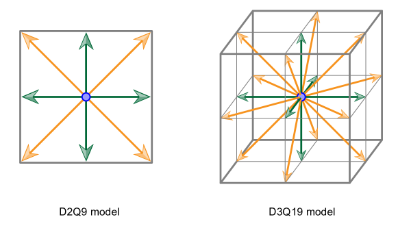
The starting point of LBM is a discretization of the position variable 𝒙𝒙{\boldsymbol{x}} by a uniform grid of cells denoted ΛΛ\Lambda, and of the momentum variable 𝒑𝒑{\boldsymbol{p}} by a small number of “velocity vectors” pointing from their current grid cell to neighboring grid cells, as illustrated in Fig. 1.
Refer to caption
Figure 1: (Color online) Illustration of the velocity vectors 𝗲isubscript𝗲𝑖{\boldsymbol{\mathsf{e}}}_{i} of the D2Q9 and D3Q19 models (adapted from [30]). All arrows and the blue circle are associated with matrix-valued distribution functions 𝖶i(𝒙,t)subscript𝖶𝑖𝒙𝑡\mathsf{W}_{i}({\boldsymbol{x}},t) in the present framework.

Here we focus on the most commonly used lattice Boltzmann models, namely D2Q9 and D3Q19 illustrated in Fig. 1. The velocity vectors are enumerated as 𝗲idsubscript𝗲𝑖superscript𝑑{\boldsymbol{\mathsf{e}}}_{i}\in\mathbb{R}^{d}, i=1,,b𝑖1𝑏i=1,\dots,b with b=9𝑏9b=9 for the D2Q9 model and b=19𝑏19b=19 for the D3Q19 model. In our case, each velocity vector within a grid cell is associated with a Wigner matrix 𝖶i(𝒙,t)2subscript𝖶𝑖𝒙𝑡subscript2\mathsf{W}_{i}({\boldsymbol{x}},t)\in\mathcal{M}_{2}, which can be interpreted as the average spin density at cell 𝒙𝒙{\boldsymbol{x}} with momentum 𝗲isubscript𝗲𝑖{\boldsymbol{\mathsf{e}}}_{i} at time t𝑡t. For simplicity, we impose periodic boundary conditions on the lattice ΛΛ\Lambda in the subsequent simulations.

For the BGK approximation of the collision operator in the discrete LBM model, the exact averaging in Eq. (7), (8), (9) to obtain the moments is replaced by a multi-dimensional integration rule. In the following section 3.1, we will devise such an integration rule adapted to the Fermi-Dirac distribution and the discretized moments 𝗲isubscript𝗲𝑖{\boldsymbol{\mathsf{e}}}_{i}, i.e., the points of the integration rule are precisely the 𝗲isubscript𝗲𝑖{\boldsymbol{\mathsf{e}}}_{i}. In section 3.2, we will construct a polynomial expansion of the Fermi-Dirac equilibrium distribution function WFDsubscript𝑊FDW_{\mathrm{FD}} compatible with the integration rule, which has the same moments as WFDsubscript𝑊FDW_{\mathrm{FD}}. The polynomial equilibrium function is required by the discrete version of the BGK collision operator, as explained in section 3.3.

3.1 Multidimensional numerical integration with Fermi-Dirac weight

Let us consider the following d𝑑d-dimensional integral

I[h]=1nd,β,μdh(𝒑)(eβ(12𝒑2μ)+1)1d𝒑𝐼delimited-[]1subscript𝑛𝑑𝛽𝜇subscriptsuperscript𝑑𝒑superscriptsuperscripte𝛽12superscript𝒑2𝜇11differential-d𝒑I[h]=\frac{1}{n_{d,\beta,\mu}}\int_{\mathbb{R}^{d}}h({\boldsymbol{p}})\left(\mathrm{e}^{\beta\left(\frac{1}{2}{\boldsymbol{p}}^{2}-\mu\right)}+1\right)^{-1}\mathrm{d}{\boldsymbol{p}} (30)

for a given (smooth) function h:d:superscript𝑑h:\mathbb{R}^{d}\to\mathbb{R}. Numerical approximations are typically of the form

I[h]Q[h]=i=1Nwih(𝒑(i)),𝐼delimited-[]𝑄delimited-[]superscriptsubscript𝑖1𝑁subscript𝑤𝑖superscript𝒑𝑖I[h]\approx Q[h]=\sum_{i=1}^{N}w_{i}\,h\big{(}{\boldsymbol{p}}^{(i)}\big{)}, (31)

with weights wisubscript𝑤𝑖w_{i}\in\mathbb{R} and points 𝒑(i)dsuperscript𝒑𝑖superscript𝑑{\boldsymbol{p}}^{(i)}\in\mathbb{R}^{d} independent of hh. For d2𝑑2d\geq 2, Q[h]𝑄delimited-[]Q[h] is denoted a cubature (see [31, 32] and references therein). A cubature formula (31) has degree m𝑚m if it is exact for polynomials hh of algebraic degree at most m𝑚m, and not exact for at least one polynomial of degree m+1𝑚1m+1. As usual, the degree of a monomial i=1dxiαisuperscriptsubscriptproduct𝑖1𝑑superscriptsubscript𝑥𝑖subscript𝛼𝑖\prod_{i=1}^{d}x_{i}^{\alpha_{i}} with αisubscript𝛼𝑖\alpha_{i}\in\mathbb{N} is given by |𝜶|=i=1dαi𝜶superscriptsubscript𝑖1𝑑subscript𝛼𝑖\lvert{\boldsymbol{\alpha}}\rvert=\sum_{i=1}^{d}\alpha_{i}, and the degree of a polynomial by the highest degree of its composing monomials. In our case, we look for fully symmetric quadrature rules [33] due to the radial symmetry of the Fermi-Dirac function, such that the moments (30) are invariant under permutations and sign changes of coordinates.

As mentioned, we identify 𝒑(i)superscript𝒑𝑖{\boldsymbol{p}}^{(i)} with the velocity vectors 𝗲isubscript𝗲𝑖{\boldsymbol{\mathsf{e}}}_{i} of the D2Q9 model for d=2𝑑2d=2 and the D3Q19 model for d=3𝑑3d=3, as illustrated in Fig. 1.

In the classical case, the Maxwell-Boltzmann distribution separates into a product of Gaussians in each dimension, and the weights associated with each discrete velocity for the D2Q9 model can be derived via the Gauss-Hermite quadrature rule of order 333 [17]. However, the Fermi-Dirac distribution does not separate into a product of functions, so the following ansatz is used.

For dimension d=2𝑑2d=2, we enumerate the 9 velocity vectors as ξ(i1,i2)2𝜉subscript𝑖1subscript𝑖2superscript2\xi\cdot(i_{1},i_{2})\in\mathbb{R}^{2} with i1,i2{1,0,1}subscript𝑖1subscript𝑖2101i_{1},i_{2}\in\{-1,0,1\} and ξ>0𝜉subscriptabsent0\xi\in\mathbb{R}_{>0}. The corresponding weights are labeled w𝒊>0subscript𝑤𝒊subscriptabsent0w_{{\boldsymbol{i}}}\in\mathbb{R}_{>0}. Our goal is to determine ξ𝜉\xi and w𝒊subscript𝑤𝒊w_{{\boldsymbol{i}}} such that

1n2,β,μ2h(𝒑)(eβ(12𝒑2μ)+1)1d𝒑i1,i2{1,0,1}w𝒊h(ξ𝒊)1subscript𝑛2𝛽𝜇subscriptsuperscript2𝒑superscriptsuperscripte𝛽12superscript𝒑2𝜇11differential-d𝒑subscriptsubscript𝑖1subscript𝑖2101subscript𝑤𝒊𝜉𝒊\frac{1}{n_{2,\beta,\mu}}\int_{\mathbb{R}^{2}}h({\boldsymbol{p}})\left(\mathrm{e}^{\beta\left(\frac{1}{2}{\boldsymbol{p}}^{2}-\mu\right)}+1\right)^{-1}\mathrm{d}{\boldsymbol{p}}\approx\sum_{i_{1},i_{2}\in\{-1,0,1\}}w_{{\boldsymbol{i}}}\,h(\xi\,{\boldsymbol{i}}) (32)

for smooth functions h:2:superscript2h:\mathbb{R}^{2}\to\mathbb{R}, with equality for polynomials up to order 555. Due to symmetry, wi1,i2=wi2,i1subscript𝑤subscript𝑖1subscript𝑖2subscript𝑤subscript𝑖2subscript𝑖1w_{i_{1},i_{2}}=w_{i_{2},i_{1}} and wi1,i2=wi1,i2subscript𝑤subscript𝑖1subscript𝑖2subscript𝑤superscriptsubscript𝑖1superscriptsubscript𝑖2w_{i_{1},i_{2}}=w_{i_{1}^{\prime},i_{2}^{\prime}} when i1=±i1subscript𝑖1plus-or-minussuperscriptsubscript𝑖1i_{1}=\pm i_{1}^{\prime} and i2=±i2subscript𝑖2plus-or-minussuperscriptsubscript𝑖2i_{2}=\pm i_{2}^{\prime}, so only the weights w00,w01,w11subscript𝑤00subscript𝑤01subscript𝑤11w_{00},w_{01},w_{11} and the length ξ𝜉\xi need to be determined. With the analytic solution

w00=15a,w01=a,w11=a4,a=F1(βμ)29F0(βμ)F2(βμ),ξ=(3βF2(βμ)F1(βμ))1/2,formulae-sequencesubscript𝑤0015𝑎formulae-sequencesubscript𝑤01𝑎formulae-sequencesubscript𝑤11𝑎4formulae-sequence𝑎subscript𝐹1superscript𝛽𝜇29subscript𝐹0𝛽𝜇subscript𝐹2𝛽𝜇𝜉superscript3𝛽subscript𝐹2𝛽𝜇subscript𝐹1𝛽𝜇12w_{00}=1-5a,\quad w_{01}=a,\quad w_{11}=\frac{a}{4},\quad a=\frac{F_{1}(\beta\mu)^{2}}{9\,F_{0}(\beta\mu)F_{2}(\beta\mu)},\quad\xi=\left(\frac{3}{\beta}\frac{F_{2}(\beta\mu)}{F_{1}(\beta\mu)}\right)^{1/2}, (33)

the approximation (32) becomes indeed exact for polynomials up to order 555, i.e., for all h(𝒑)=p1m1p2m2𝒑superscriptsubscript𝑝1subscript𝑚1superscriptsubscript𝑝2subscript𝑚2h({\boldsymbol{p}})=p_{1}^{m_{1}}\,p_{2}^{m_{2}} with m1+m25subscript𝑚1subscript𝑚25m_{1}+m_{2}\leq 5. Note that all odd moments vanish due to the even symmetry of the Fermi-Dirac distribution.

For μ=0𝜇0\mu=0, the parameters in Eq. (33) simplify to

a=π4972ζ(3)log(2)0.120277,ξ=3π(3ζ(3)β)1/21.8134β,formulae-sequence𝑎superscript𝜋4972𝜁32approaches-limit0.120277𝜉3𝜋superscript3𝜁3𝛽12approaches-limit1.8134𝛽a=\frac{\pi^{4}}{972\,\zeta(3)\log(2)}\doteq 0.120277,\quad\xi=\frac{3}{\pi}\left(\frac{3\,\zeta(3)}{\beta}\right)^{1/2}\doteq\frac{1.8134}{\sqrt{\beta}}, (34)

where ζ(s)𝜁𝑠\zeta(s) is the Riemann zeta function.

For dimension d=3𝑑3d=3, one can proceed analogously. We enumerate the points ξ(i1,i2,i3)3𝜉subscript𝑖1subscript𝑖2subscript𝑖3superscript3\xi\cdot(i_{1},i_{2},i_{3})\in\mathbb{R}^{3} and weights w𝒊>0subscript𝑤𝒊subscriptabsent0w_{{\boldsymbol{i}}}\in\mathbb{R}_{>0} of the D3Q19 model (on the right in Fig. 1) using the indices i1,i2,i3{1,0,1}subscript𝑖1subscript𝑖2subscript𝑖3101i_{1},i_{2},i_{3}\in\{-1,0,1\}, with the additional constraint that |i1|+|i2|+|i3|2subscript𝑖1subscript𝑖2subscript𝑖32\lvert i_{1}\rvert+\lvert i_{2}\rvert+\lvert i_{3}\rvert\leq 2 due to the missing cell corners in the D3Q19 model. The goal is an approximation

1n3,β,μ3h(𝒑)(eβ(12𝒑2μ)+1)1d𝒑𝒊D3Q19w𝒊h(ξ𝒊),1subscript𝑛3𝛽𝜇subscriptsuperscript3𝒑superscriptsuperscripte𝛽12superscript𝒑2𝜇11differential-d𝒑subscript𝒊D3Q19subscript𝑤𝒊𝜉𝒊\frac{1}{n_{3,\beta,\mu}}\int_{\mathbb{R}^{3}}h({\boldsymbol{p}})\left(\mathrm{e}^{\beta\left(\frac{1}{2}{\boldsymbol{p}}^{2}-\mu\right)}+1\right)^{-1}\mathrm{d}{\boldsymbol{p}}\approx\sum_{{\boldsymbol{i}}\in\mathrm{D3Q19}}w_{{\boldsymbol{i}}}\,h(\xi\,{\boldsymbol{i}}), (35)

such that equality holds for polynomials hh up to order 555. Again due to symmetry, only the weights w000,w001,w011subscript𝑤000subscript𝑤001subscript𝑤011w_{000},w_{001},w_{011} and the length ξ𝜉\xi need to be determined. A short calculation results in the analytic solution

w000=112a,w001=a,w011=a2,a=F3/2(βμ)218F1/2(βμ)F5/2(βμ);ξ=(3βF5/2(βμ)F3/2(βμ))1/2.\begin{split}w_{000}&=1-12a,\quad w_{001}=a,\quad w_{011}=\frac{a}{2},\quad a=\frac{F_{3/2}(\beta\mu)^{2}}{18\,F_{1/2}(\beta\mu)\,F_{5/2}(\beta\mu)};\\ \xi&=\left(\frac{3}{\beta}\frac{F_{5/2}(\beta\mu)}{F_{3/2}(\beta\mu)}\right)^{1/2}.\end{split} (36)

Evaluated at μ=0𝜇0\mu=0, the parameters in Eq. (36) simplify to

a=(41+92)ζ(52)2558ζ(32)ζ(72)0.0588684,ξ=(3β(15+22)ζ(72)14ζ(52))1/21.79131β.formulae-sequence𝑎4192𝜁superscript522558𝜁32𝜁72approaches-limit0.0588684𝜉superscript3𝛽1522𝜁7214𝜁5212approaches-limit1.79131𝛽a=\frac{\left(41+9\sqrt{2}\right)\zeta(\frac{5}{2})^{2}}{558\,\zeta(\frac{3}{2})\,\zeta(\frac{7}{2})}\doteq 0.0588684,\quad\xi=\left(\frac{3}{\beta}\frac{\left(15+2\sqrt{2}\right)\zeta(\frac{7}{2})}{14\,\zeta(\frac{5}{2})}\right)^{1/2}\doteq\frac{1.79131}{\sqrt{\beta}}. (37)

In the following, the inverse temperature and chemical potential of the integration rule are denoted by β0subscript𝛽0\beta_{0} and μ0subscript𝜇0\mu_{0}, respectively, to distinguish them from the physical quantities. According to Eq. (33) and (36), the length factor ξ𝜉\xi depends on β0subscript𝛽0\beta_{0} and μ0subscript𝜇0\mu_{0}. The uniform grid of the lattice Boltzmann methods requires the same ξ𝜉\xi for all cells, which can be identified as the lattice constant. Thus we set β0subscript𝛽0\beta_{0} to a uniform, fixed value for all grid cells, and μ0=0subscript𝜇00\mu_{0}=0. Different from that, the physical quantities β𝛽\beta, μsubscript𝜇\mu_{\uparrow} and μsubscript𝜇\mu_{\downarrow} of the equilibrium function associated with a grid cell can vary across cells (see the following section 3.2). An alternative route (not pursued in the present paper) would be an isothermal model, where β=β0𝛽subscript𝛽0\beta=\beta_{0} is held fixed for all grid cells and time steps. The main disadvantage of this approach is the loss of the energy conservation in the simulation. Note that isothermal models are typically used in “classical” lattice Boltzmann methods [17].

The integration rule replaces the analytic integrals in Eq. (7), (8) and (9) for the local density, velocity and energy by the discrete analogues (at given 𝒙,t𝒙𝑡{\boldsymbol{x}},t)

ρ=i=1b𝖶i(𝒙,t),tr[ρ]𝒖=i=1b𝗲itr[𝖶i(𝒙,t)],tr[ρ]ε=i=1b12|𝗲i𝒖|2tr[𝖶i(𝒙,t)].formulae-sequence𝜌superscriptsubscript𝑖1𝑏subscript𝖶𝑖𝒙𝑡formulae-sequencetr𝜌𝒖superscriptsubscript𝑖1𝑏subscript𝗲𝑖trsubscript𝖶𝑖𝒙𝑡tr𝜌𝜀superscriptsubscript𝑖1𝑏12superscriptsubscript𝗲𝑖𝒖2trsubscript𝖶𝑖𝒙𝑡\rho=\sum_{i=1}^{b}\mathsf{W}_{i}({\boldsymbol{x}},t),\quad\operatorname{tr}[\rho]\,{\boldsymbol{u}}=\sum_{i=1}^{b}{\boldsymbol{\mathsf{e}}}_{i}\operatorname{tr}[\mathsf{W}_{i}({\boldsymbol{x}},t)],\quad\operatorname{tr}[\rho]\,\varepsilon=\sum_{i=1}^{b}\tfrac{1}{2}\lvert{\boldsymbol{\mathsf{e}}}_{i}-{\boldsymbol{u}}\rvert^{2}\operatorname{tr}[\mathsf{W}_{i}({\boldsymbol{x}},t)]. (38)

By convention, the integration weights wisubscript𝑤𝑖w_{i} are already absorbed into the discretized Wigner functions 𝖶i(𝒙,t)subscript𝖶𝑖𝒙𝑡\mathsf{W}_{i}({\boldsymbol{x}},t).

3.2 Polynomial expansion of the equilibrium distribution function

Our goal is to construct an approximate equilibrium distribution function compatible with the quadrature formula Eq. (32) at μ=0𝜇0\mu=0, such that its moments agree with the exact Fermi-Dirac values (18), (20) and the average velocity 𝒖𝒖{\boldsymbol{u}}. The following ansatz is used:

W(eq)(𝒑)=1nd,β0,0(eβ012𝒑2+1)1U(nd,β,μ00nd,β,μ)U×(α1+α2β012𝒑2+α3β0(𝒑𝒖)+α4(β0𝒑𝒖)2+α5β012𝒖2),superscript𝑊eq𝒑1subscript𝑛𝑑subscript𝛽00superscriptsuperscriptesubscript𝛽012superscript𝒑211𝑈matrixsubscript𝑛𝑑𝛽subscript𝜇00subscript𝑛𝑑𝛽subscript𝜇superscript𝑈subscript𝛼1subscript𝛼2subscript𝛽012superscript𝒑2subscript𝛼3subscript𝛽0𝒑𝒖subscript𝛼4superscriptsubscript𝛽0𝒑𝒖2subscript𝛼5subscript𝛽012superscript𝒖2W^{(\mathrm{eq})}({\boldsymbol{p}})=\frac{1}{n_{d,\beta_{0},0}}\left(\mathrm{e}^{\beta_{0}\frac{1}{2}{\boldsymbol{p}}^{2}}+1\right)^{-1}U\begin{pmatrix}n_{d,\beta,\mu_{\uparrow}}&0\\ 0&n_{d,\beta,\mu_{\downarrow}}\end{pmatrix}U^{*}\\ \times\Big{(}\alpha_{1}+\alpha_{2}\,\beta_{0}\,\tfrac{1}{2}{\boldsymbol{p}}^{2}+\alpha_{3}\,\beta_{0}\,({\boldsymbol{p}}\cdot{\boldsymbol{u}})+\alpha_{4}(\beta_{0}\,{\boldsymbol{p}}\cdot{\boldsymbol{u}})^{2}+\alpha_{5}\,\beta_{0}\,\tfrac{1}{2}{\boldsymbol{u}}^{2}\Big{)}, (39)

with the coefficients αisubscript𝛼𝑖\alpha_{i} to be determined. Note that μ𝜇\mu has disappeared from the exponent in Eq. (39), as required by the quadrature rule mentioned above. A solution for the coefficients in dimensions d=2𝑑2d=2 and d=3𝑑3d=3 is provided in the appendix. It turns out that α3subscript𝛼3\alpha_{3}, α4subscript𝛼4\alpha_{4} and α5subscript𝛼5\alpha_{5} are constants, and α1subscript𝛼1\alpha_{1}, α2subscript𝛼2\alpha_{2} only depend on β0εFDsubscript𝛽0subscript𝜀FD\beta_{0}\,\varepsilon_{\mathrm{FD}}, i.e., β0subscript𝛽0\beta_{0} times the average internal energy defined in Eq. (20). This dependence and being matrix-valued is the main difference to the conventional equilibrium function used in the classical lattice Boltzmann method; otherwise, the expression (39) formally resembles the classical counterpart.
Refer to caption
(a) d=2𝑑2d=2, β0=0.8subscript𝛽00.8\beta_{0}=0.8
Refer to caption
(b) d=3𝑑3d=3, β0=0.8subscript𝛽00.8\beta_{0}=0.8
Refer to caption
(c) d=2𝑑2d=2, β0=1.2subscript𝛽01.2\beta_{0}=1.2
Refer to caption
(d) d=3𝑑3d=3, β0=1.2subscript𝛽01.2\beta_{0}=1.2
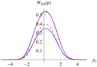
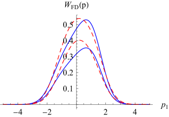
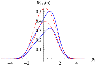
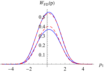
Figure 2: (Color online) Diagonal matrix entries of the polynomial approximation in Eq. (39) with U=𝟙𝑈1U=\mathbbm{1} (blue solid curves) compared to the exact Fermi-Dirac equilibrium distribution WFDsubscript𝑊FDW_{\mathrm{FD}} defined in Eq. (5) with ω(𝒑)=12|𝒑|2𝜔𝒑12superscript𝒑2\omega({\boldsymbol{p}})=\frac{1}{2}\lvert{\boldsymbol{p}}\rvert^{2} (dashed red), for d=2𝑑2d=2 (left column) and d=3𝑑3d=3 (right column).

Note that the approximation (39) of WFDsubscript𝑊FDW_{\mathrm{FD}} is per se independent of the quadrature formula constructed in section 3.1. In particular, the moments of W(eq)superscript𝑊eqW^{(\mathrm{eq})} can be calculated by continuous integration, according to Eq. (7), (8) and (9). But of course the structure of W(eq)superscript𝑊eqW^{(\mathrm{eq})} allows us to obtain the exact same moments using the quadrature formula from section 3.1.

Fig. 2 compares the approximation (39) with the exact Fermi-Dirac function WFDsubscript𝑊FDW_{\mathrm{FD}}, both for d=2𝑑2d=2 and d=3𝑑3d=3. The upper row differs from the lower solely by β0subscript𝛽0\beta_{0}, the “reference” inverse temperature used in the weight function of the numerical integration rule. The functions are plotted along the p1subscript𝑝1p_{1} axis through the origin. The parameters defining the distribution function read β=1𝛽1\beta=1, μ=0.2subscript𝜇0.2\mu_{\uparrow}=0.2, μ=0.35subscript𝜇0.35\mu_{\downarrow}=-0.35, 𝒖=(0.2,0.3)𝒖0.20.3{\boldsymbol{u}}=(0.2,0.3) for d=2𝑑2d=2 and 𝒖=(0.2,0.3,0.2)𝒖0.20.30.2{\boldsymbol{u}}=(0.2,0.3,-0.2) for d=3𝑑3d=3. One notices the larger deviation from the exact curve as β0subscript𝛽0\beta_{0} overshoots the physical β𝛽\beta, a feature which seems to be systematic for the polynomial approximation.

In terms of the velocity vectors 𝗲isubscript𝗲𝑖{\boldsymbol{\mathsf{e}}}_{i}, the equilibrium function (39) evaluated at these points times the corresponding weight wisubscript𝑤𝑖w_{i} gives the discretized equilibrium distribution function

𝖶i(eq)=wiU(nd,β,μ00nd,β,μ)U×(α1+α2β012𝗲i2+α3β0(𝗲i𝒖)+α4(β0𝗲i𝒖)2+α5β012𝒖2),subscriptsuperscript𝖶eq𝑖subscript𝑤𝑖𝑈matrixsubscript𝑛𝑑𝛽subscript𝜇00subscript𝑛𝑑𝛽subscript𝜇superscript𝑈subscript𝛼1subscript𝛼2subscript𝛽012superscriptsubscript𝗲𝑖2subscript𝛼3subscript𝛽0subscript𝗲𝑖𝒖subscript𝛼4superscriptsubscript𝛽0subscript𝗲𝑖𝒖2subscript𝛼5subscript𝛽012superscript𝒖2\mathsf{W}^{(\mathrm{eq})}_{i}=w_{i}\,U\begin{pmatrix}n_{d,\beta,\mu_{\uparrow}}&0\\ 0&n_{d,\beta,\mu_{\downarrow}}\end{pmatrix}U^{*}\\ \times\Big{(}\alpha_{1}+\alpha_{2}\,\beta_{0}\,\tfrac{1}{2}{\boldsymbol{\mathsf{e}}}_{i}^{2}+\alpha_{3}\,\beta_{0}\,({\boldsymbol{\mathsf{e}}}_{i}\cdot{\boldsymbol{u}})+\alpha_{4}(\beta_{0}\,{\boldsymbol{\mathsf{e}}}_{i}\cdot{\boldsymbol{u}})^{2}+\alpha_{5}\,\beta_{0}\,\tfrac{1}{2}{\boldsymbol{u}}^{2}\Big{)}, (40)

which will be used in the subsequent lattice Boltzmann simulation.

The approximate polynomial equilibrium function constructed so far has the drawback that the last factor in Eq. (40) can become negative for certain values of β𝛽\beta, μsubscript𝜇\mu_{\uparrow}, μsubscript𝜇\mu_{\downarrow} and 𝒖𝒖{\boldsymbol{u}}, resulting in an (unphysical) 𝖶i(eq)subscriptsuperscript𝖶eq𝑖\mathsf{W}^{(\mathrm{eq})}_{i} with negative eigenvalues. This issue is discussed in the following section.

3.3 Quantum lattice Boltzmann method

Using the results from Sec. 3.1 and 3.2, we can now specify the details of the numerical framework using the BGK collision operator. The framework takes as input the relaxation time τ𝜏\tau and a reference inverse temperature β0subscript𝛽0\beta_{0} (globally constant) for the numerical integration (see section 3.1). The weights wisubscript𝑤𝑖w_{i} and length parameter ξ𝜉\xi can then be precomputed according to Eq. (34) for d=2𝑑2d=2 and Eq. (37) for d=3𝑑3d=3. The transport step in Eq. (43) below relates ξ𝜉\xi to the time step ΔtΔ𝑡\Delta t and lattice cell width ΔxΔ𝑥\Delta x via Δtξ=ΔxΔ𝑡𝜉Δ𝑥\Delta t\,\xi=\Delta x. Furthermore, an initial configuration of distribution functions 𝖶i(𝒙,t0)subscript𝖶𝑖𝒙subscript𝑡0\mathsf{W}_{i}({\boldsymbol{x}},t_{0}) is required as input.

The framework approximates the kinetics of the Boltzmann equation by performing the following calculations for each discrete time step tt+Δt𝑡𝑡Δ𝑡t\to t+\Delta t:

  • For each cell 𝒙𝒙{\boldsymbol{x}}, the local average momentum ρ𝜌\rho, velocity 𝒖𝒖{\boldsymbol{u}} and energy ε𝜀\varepsilon of 𝖶i(𝒙,t)subscript𝖶𝑖𝒙𝑡\mathsf{W}_{i}({\boldsymbol{x}},t) are calculated according to Eq. (38). These averages define the local equilibrium function

    𝖶i(eq)=wiρ(α1+α2β012𝗲i2+α3β0(𝗲i𝒖)+α4(β0𝗲i𝒖)2+α5β012𝒖2),subscriptsuperscript𝖶eq𝑖subscript𝑤𝑖𝜌subscript𝛼1subscript𝛼2subscript𝛽012superscriptsubscript𝗲𝑖2subscript𝛼3subscript𝛽0subscript𝗲𝑖𝒖subscript𝛼4superscriptsubscript𝛽0subscript𝗲𝑖𝒖2subscript𝛼5subscript𝛽012superscript𝒖2\mathsf{W}^{(\mathrm{eq})}_{i}=w_{i}\,\rho\,\Big{(}\alpha_{1}+\alpha_{2}\,\beta_{0}\,\tfrac{1}{2}{\boldsymbol{\mathsf{e}}}_{i}^{2}+\alpha_{3}\,\beta_{0}\,({\boldsymbol{\mathsf{e}}}_{i}\cdot{\boldsymbol{u}})+\alpha_{4}(\beta_{0}\,{\boldsymbol{\mathsf{e}}}_{i}\cdot{\boldsymbol{u}})^{2}+\alpha_{5}\,\beta_{0}\,\tfrac{1}{2}{\boldsymbol{u}}^{2}\Big{)}, (41)

    with the coefficients αjsubscript𝛼𝑗\alpha_{j} provided in the appendix (setting εFD=εsubscript𝜀FD𝜀\varepsilon_{\mathrm{FD}}=\varepsilon). The unitary matrix U𝑈U appearing in Eq. (40) does not need to be computed, nor any Fermi-Dirac integral function Fk(x)subscript𝐹𝑘𝑥F_{k}(x).

  • Collision: for each cell 𝒙𝒙{\boldsymbol{x}}, the discretized BGK collision operator is applied to obtain the post-collisional distribution function 𝖶icoll(𝒙,t)subscriptsuperscript𝖶coll𝑖𝒙𝑡\mathsf{W}^{\mathrm{coll}}_{i}({\boldsymbol{x}},t):

    𝖶icoll(𝒙,t)=𝖶i(𝒙,t)+Δtτ(𝖶i(eq)𝖶i(𝒙,t)),subscriptsuperscript𝖶coll𝑖𝒙𝑡subscript𝖶𝑖𝒙𝑡Δ𝑡𝜏subscriptsuperscript𝖶eq𝑖subscript𝖶𝑖𝒙𝑡\mathsf{W}^{\mathrm{coll}}_{i}({\boldsymbol{x}},t)=\mathsf{W}_{i}({\boldsymbol{x}},t)+\frac{\Delta t}{\tau}\left(\mathsf{W}^{\mathrm{(eq)}}_{i}-\mathsf{W}_{i}({\boldsymbol{x}},t)\right), (42)

    with 𝖶i(eq)subscriptsuperscript𝖶eq𝑖\mathsf{W}^{\mathrm{(eq)}}_{i} defined in Eq. (41).

  • Streaming: the distribution functions are transported along their respective velocity directions 𝗲isubscript𝗲𝑖{\boldsymbol{\mathsf{e}}}_{i}:

    𝖶i(𝒙+Δt𝗲i,t+Δt)=𝖶icoll(𝒙,t)subscript𝖶𝑖𝒙Δ𝑡subscript𝗲𝑖𝑡Δ𝑡subscriptsuperscript𝖶coll𝑖𝒙𝑡\mathsf{W}_{i}({\boldsymbol{x}}+\Delta t\,{\boldsymbol{\mathsf{e}}}_{i},t+\Delta t)=\mathsf{W}^{\mathrm{coll}}_{i}({\boldsymbol{x}},t) (43)

    for all i=1,,b𝑖1𝑏i=1,\dots,b and cells 𝒙𝒙{\boldsymbol{x}}. This step approximates the transport term
    𝒑𝒙W(𝒑,𝒙,t)𝒑subscriptbold-∇𝒙𝑊𝒑𝒙𝑡{\boldsymbol{p}}\cdot{\boldsymbol{\nabla}}_{{\boldsymbol{x}}}W({\boldsymbol{p}},{\boldsymbol{x}},t) in the Boltzmann equation (1).

The numerical operations required by the algorithm are relatively simple, and the Fermi-Dirac integral functions Fk(x)subscript𝐹𝑘𝑥F_{k}(x) need not be evaluated.

To compensate for potentially negative-definite, unphysical 𝖶i(eq)subscriptsuperscript𝖶eq𝑖\mathsf{W}^{(\mathrm{eq})}_{i} in (41), one could dynamically decrease 1τ1𝜏\frac{1}{\tau} in (42) such that 𝖶icoll(𝒙,t)subscriptsuperscript𝖶coll𝑖𝒙𝑡\mathsf{W}^{\mathrm{coll}}_{i}({\boldsymbol{x}},t) is guaranteed to be positive semidefinite. However, this could lead to 1τ01𝜏0\frac{1}{\tau}\to 0, such that the simulation effectively halts. We have therefore avoided this adjustment; for the numerical examples in Sec. 4, negative-definite distribution functions appear rarely and do not seem to affect the simulation results.

Importantly, the numerical scheme preserves the local, discrete versions of the density, momentum and energy conservation laws. For periodic boundary conditions without external forces, it follows that the global average density, velocity and total energy

ρ(t)𝜌𝑡\displaystyle\rho(t) =1|Λ|𝒙Λρ(𝒙,t)=1|Λ|𝒙Λi=1b𝖶i(𝒙,t),absent1Λsubscript𝒙Λ𝜌𝒙𝑡1Λsubscript𝒙Λsuperscriptsubscript𝑖1𝑏subscript𝖶𝑖𝒙𝑡\displaystyle=\frac{1}{\lvert\Lambda\rvert}\sum_{{\boldsymbol{x}}\in\Lambda}\rho({\boldsymbol{x}},t)=\frac{1}{\lvert\Lambda\rvert}\sum_{{\boldsymbol{x}}\in\Lambda}\sum_{i=1}^{b}\mathsf{W}_{i}({\boldsymbol{x}},t), (44)
tr[ρ(t)]𝒖(t)tr𝜌𝑡𝒖𝑡\displaystyle\operatorname{tr}[\rho(t)]\,{\boldsymbol{u}}(t) =1|Λ|𝒙Λtr[ρ(𝒙,t)]𝒖(𝒙,t)=1|Λ|𝒙Λi=1b𝗲itr[𝖶i(𝒙,t)],absent1Λsubscript𝒙Λtr𝜌𝒙𝑡𝒖𝒙𝑡1Λsubscript𝒙Λsuperscriptsubscript𝑖1𝑏subscript𝗲𝑖trsubscript𝖶𝑖𝒙𝑡\displaystyle=\frac{1}{\lvert\Lambda\rvert}\sum_{{\boldsymbol{x}}\in\Lambda}\operatorname{tr}[\rho({\boldsymbol{x}},t)]\,{\boldsymbol{u}}({\boldsymbol{x}},t)=\frac{1}{\lvert\Lambda\rvert}\sum_{{\boldsymbol{x}}\in\Lambda}\sum_{i=1}^{b}{\boldsymbol{\mathsf{e}}}_{i}\operatorname{tr}[\mathsf{W}_{i}({\boldsymbol{x}},t)],\quad (45)
tr[ρ(t)]εtot(t)=1|Λ|𝒙Λtr[ρ(𝒙,t)](ε(𝒙,t)+12|𝒖(𝒙,t)|2)=1|Λ|𝒙Λi=1b12|𝗲i|2tr[𝖶i(𝒙,t)]tr𝜌𝑡subscript𝜀tot𝑡1Λsubscript𝒙Λtr𝜌𝒙𝑡𝜀𝒙𝑡12superscript𝒖𝒙𝑡21Λsubscript𝒙Λsuperscriptsubscript𝑖1𝑏12superscriptsubscript𝗲𝑖2trsubscript𝖶𝑖𝒙𝑡\displaystyle\begin{split}\operatorname{tr}[\rho(t)]\,\varepsilon_{\mathrm{tot}}(t)&=\frac{1}{\lvert\Lambda\rvert}\sum_{{\boldsymbol{x}}\in\Lambda}\operatorname{tr}[\rho({\boldsymbol{x}},t)]\left(\varepsilon({\boldsymbol{x}},t)+\tfrac{1}{2}\lvert{\boldsymbol{u}}({\boldsymbol{x}},t)\rvert^{2}\right)\\ &=\frac{1}{\lvert\Lambda\rvert}\sum_{{\boldsymbol{x}}\in\Lambda}\sum_{i=1}^{b}\tfrac{1}{2}\lvert{\boldsymbol{\mathsf{e}}}_{i}\rvert^{2}\operatorname{tr}[\mathsf{W}_{i}({\boldsymbol{x}},t)]\end{split} (46)

remain constant under the numerical time evolution. Since the final (t𝑡t\to\infty) state is expected to be homogeneous (uniform in 𝒙𝒙{\boldsymbol{x}}), the the discussion following the proof of proposition 1 applies, and the average quantities (44), (45), (46) actually determine the final equilibrium state.

Notably, the analysis in [34] suggests that a discrete version of the H-theorem does not exist for the present framework.

4 Simulation and validation

Riemann problem

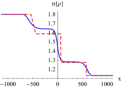
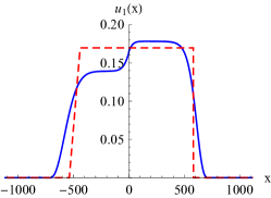
To validate the quantum LBM scheme, we compare it to an analytic solution of the Riemann problem [35] for the Euler equations (21), which are expected to be a good approximation close to thermal equilibrium.
Refer to caption
(a) density tr[ρ]tr𝜌{\operatorname{tr}[\rho]}
Refer to caption
(b) velocity
Refer to caption
(c) pressure P=(γ1)tr[ρ]ε𝑃𝛾1tr𝜌𝜀{P=(\gamma-1)\operatorname{tr}[\rho]\varepsilon}
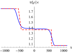
Figure 3: (Color online) Solution of a Riemann problem using the present LBM scheme after 385 time steps (blue solid curves) in comparison with a corresponding analytic solution of the Euler equations (21) (red dashed).

Specifically, the initial state consists of two thermodynamically equilibrated regions which are divided at x=0𝑥0x=0 by a virtual membrane. At t=0𝑡0t=0 the membrane is removed and the two regions start to intermingle with each other. In the left region we initially choose WFDsubscript𝑊FDW_{\mathrm{FD}} with μ=32subscript𝜇32\mu_{\uparrow}=-\frac{3}{2} and μ=52subscript𝜇52\mu_{\downarrow}=-\frac{5}{2}, and in the right region μ=2subscript𝜇2\mu_{\uparrow}=-2 and μ=3subscript𝜇3\mu_{\downarrow}=-3. The initial inverse temperature β=1𝛽1\beta=1 and velocity 𝒖=0𝒖0{\boldsymbol{u}}=0 are the same for both regions. The corresponding density and energy can be computed according to (18) and (20). The analytical solution [35] of the Euler equations depends only on the ratio xt𝑥𝑡\frac{x}{t}. With the described initial data, it consists of a shock wave traveling to the right, a contact discontinuity with a jump in density traveling also to the right at lower speed, and a rarefaction wave traveling to the left. For an ideal polytropic gas, the pressure is given by P=(γ1)tr[ρ]ε𝑃𝛾1tr𝜌𝜀P=(\gamma-1)\operatorname{tr}[\rho]\varepsilon with γ𝛾\gamma the adiabatic exponent. In our case γ=1+2d=2𝛾12𝑑2\gamma=1+\frac{2}{d}=2 since we run the quantum LBM scheme on a two-dimensional grid with dimensions 2048×2204822048\times 2 (quasi-1D) and periodic boundary conditions. The relaxation time of the collision operator was set to τ=10𝜏10\tau=10. The LBM solution is compared to the analytic Euler solution in Fig. 3. The features of the Euler solution are qualitatively reproduced, albeit with a small jump in velocity close to x=0𝑥0x=0.

Interference

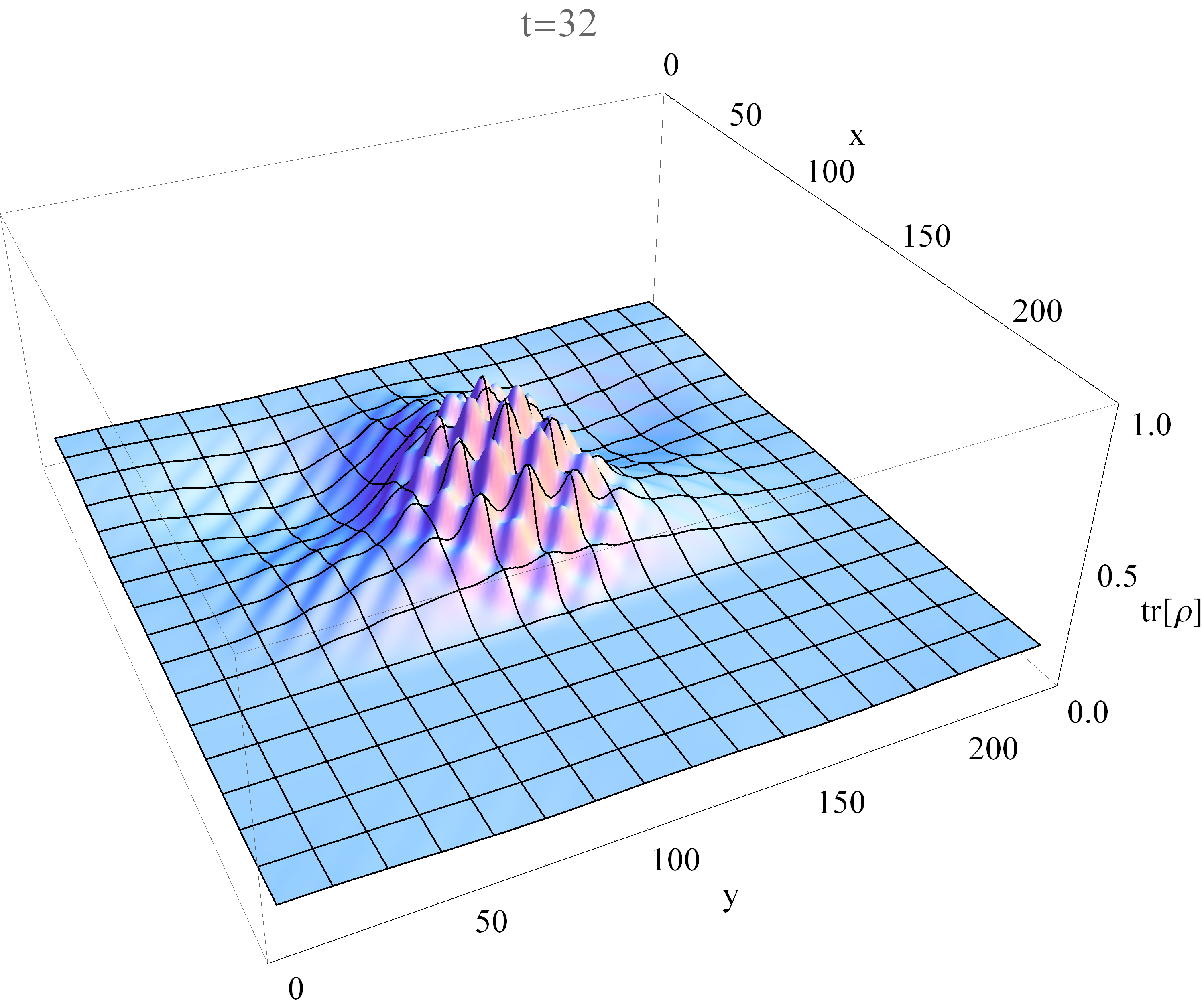
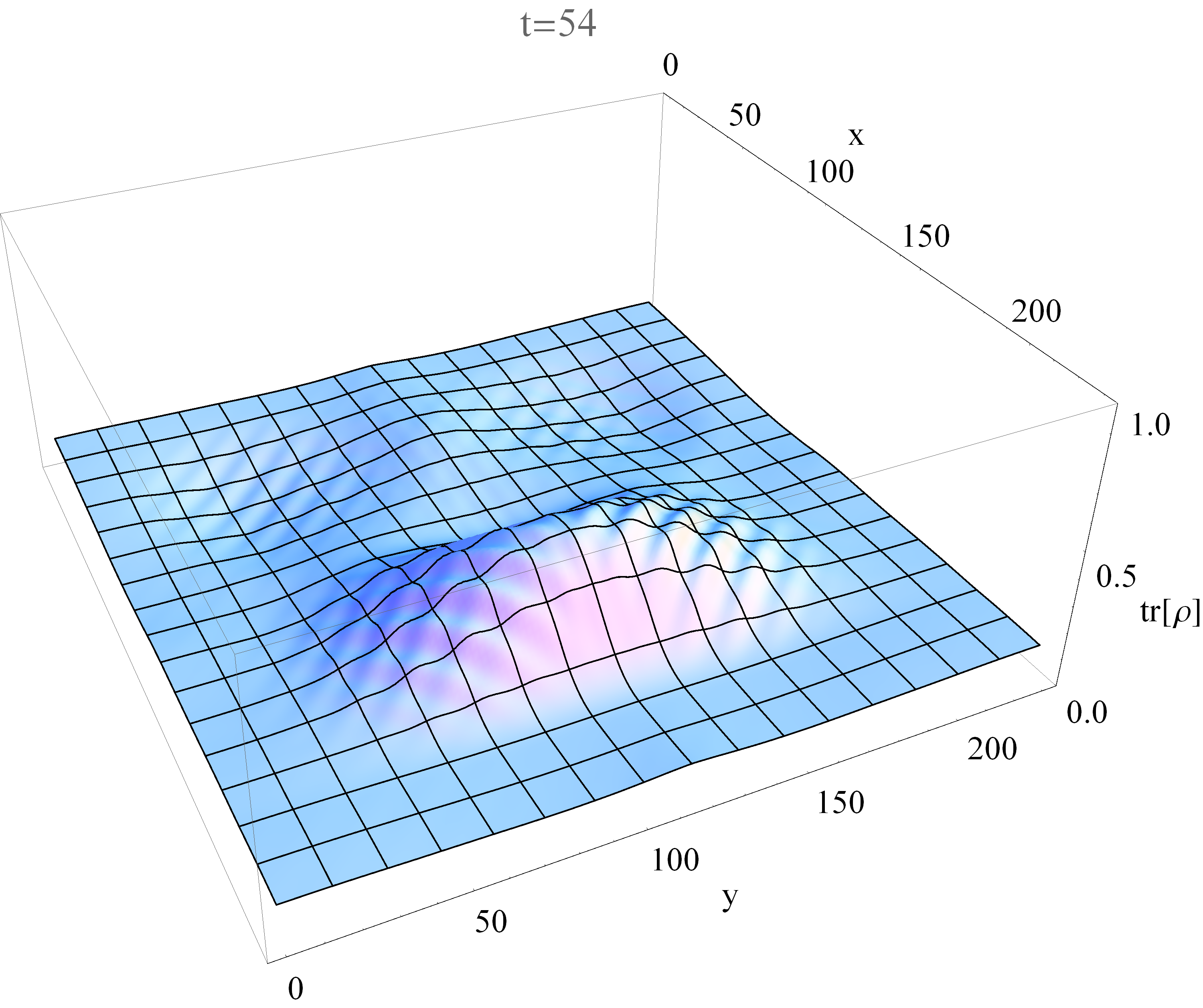
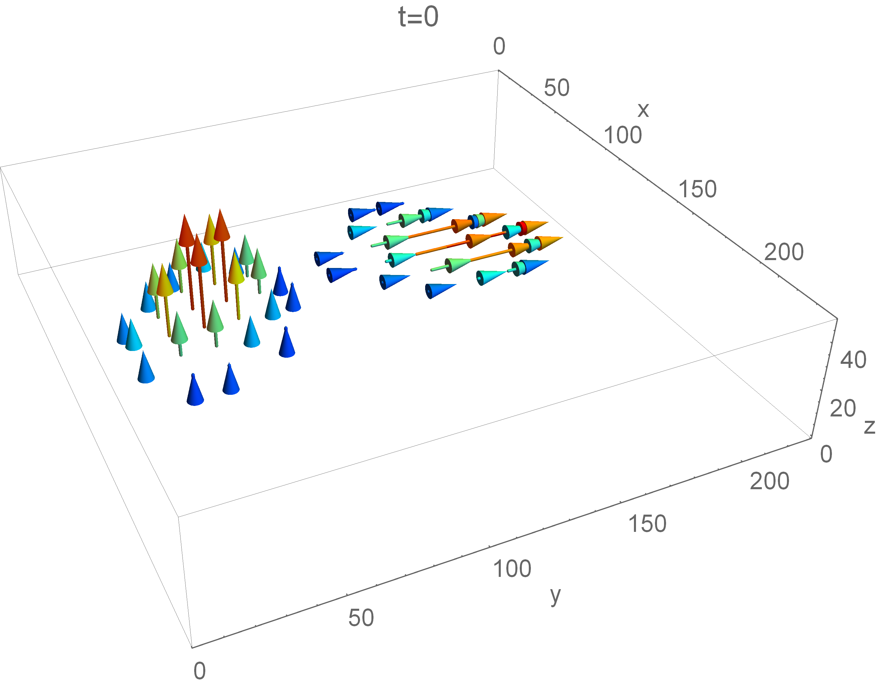
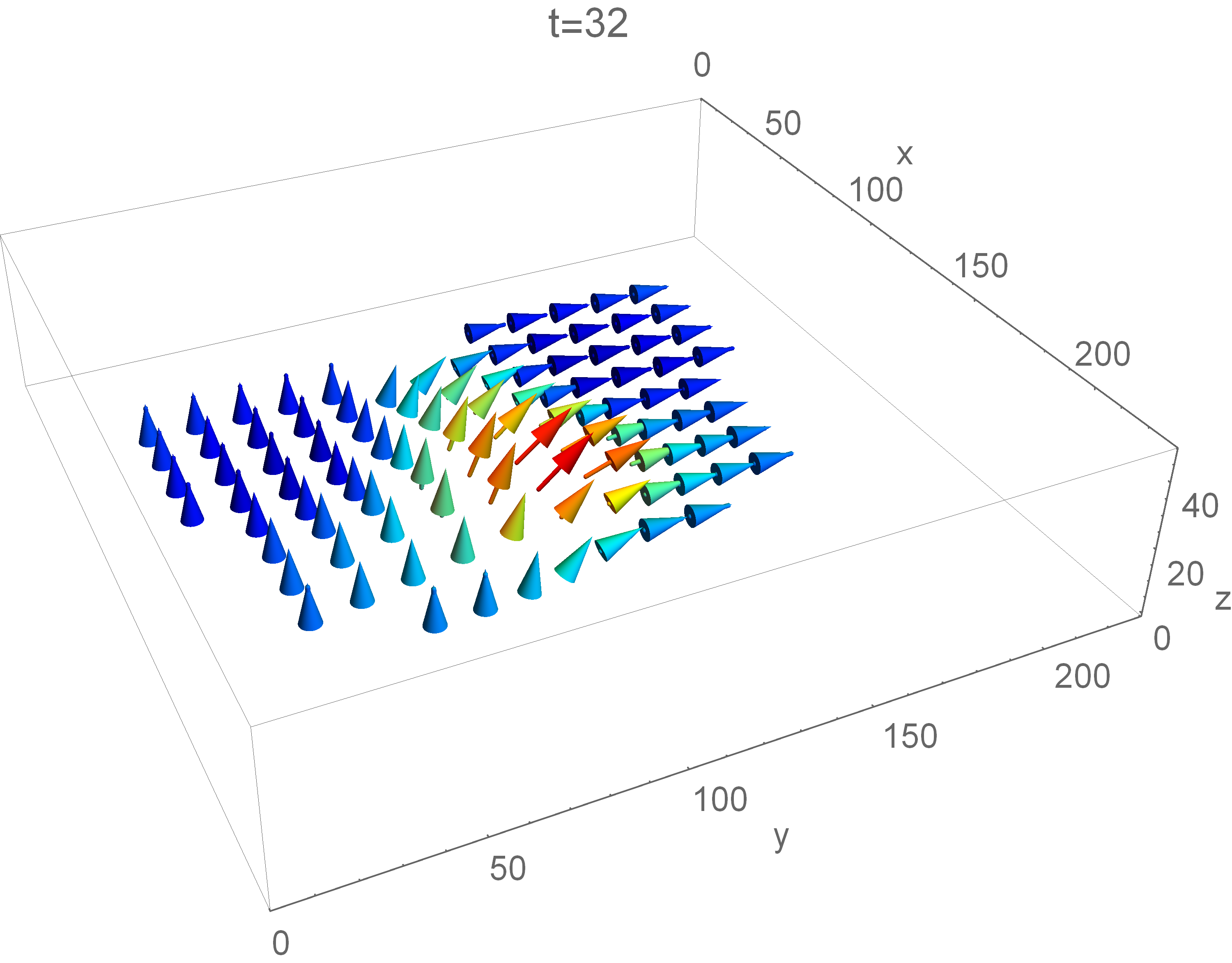
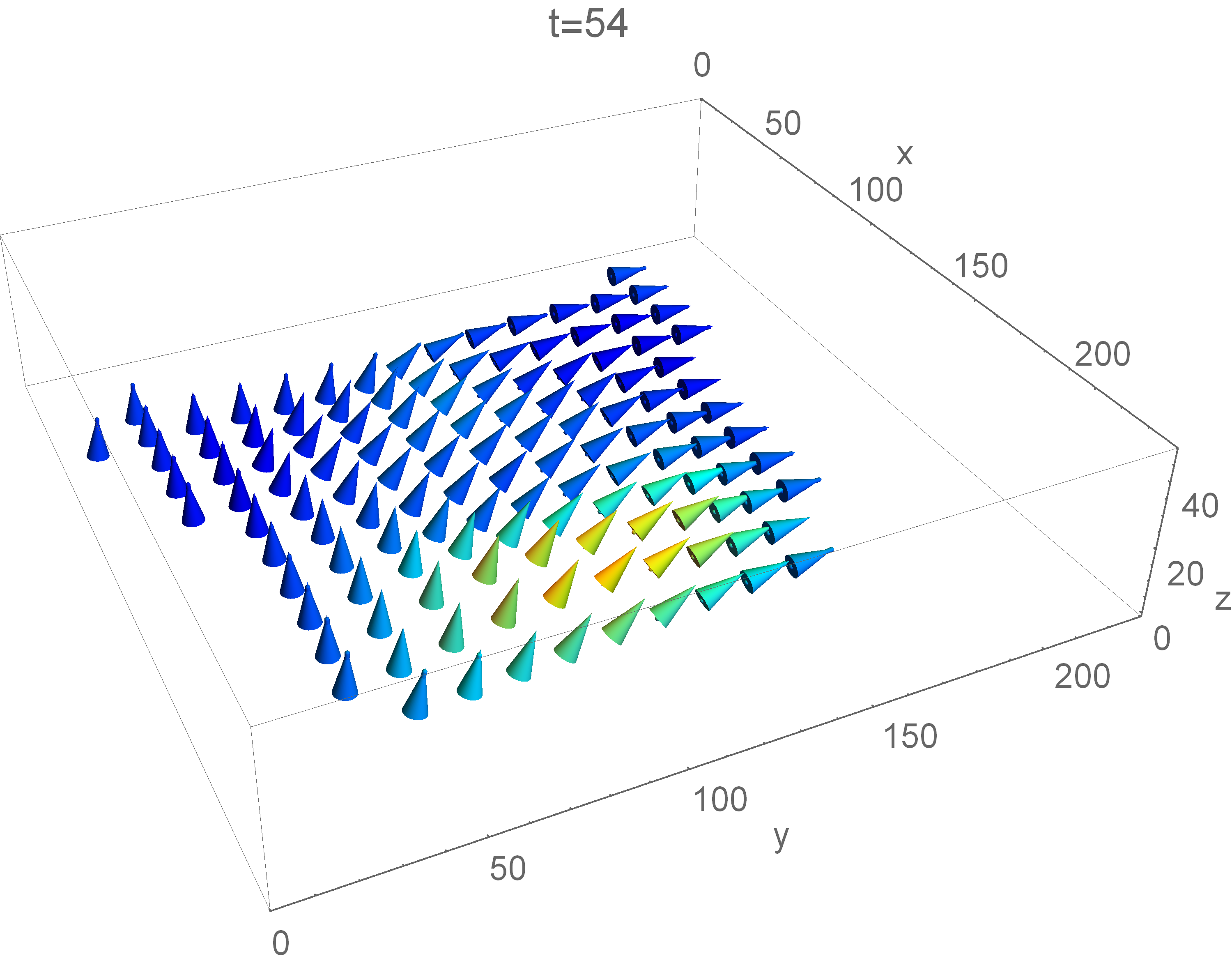
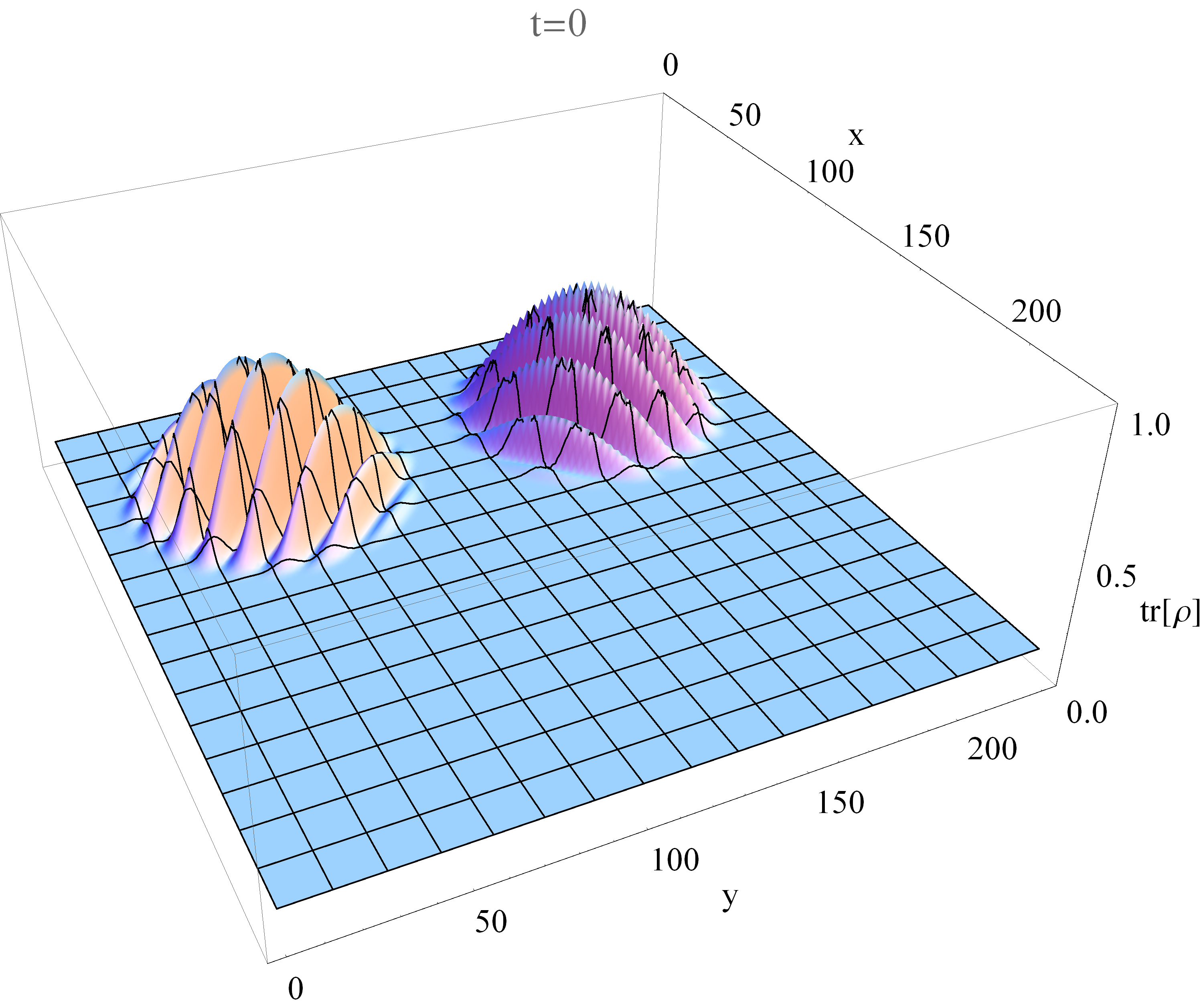
Next, we study the interference pattern emerging from the collision of two wavelet-shaped density distribution “packets” in two dimensions, as shown in Fig. 4.
Refer to caption
(a) tr[ρ]tr𝜌\operatorname{tr}[\rho] at t=0𝑡0t=0
Refer to caption
(b) tr[ρ]tr𝜌\operatorname{tr}[\rho] at time step 323232
Refer to caption
(c) tr[ρ]tr𝜌\operatorname{tr}[\rho] at time step 545454
Refer to caption
(d) Bloch vectors at t=0𝑡0t=0
Refer to caption
(e) Bloch vectors at time step 323232
Refer to caption
(f) Bloch vectors at time step 545454
Figure 4: (Color online) Collision and interference of two wavelet-shaped density distributions with different spin orientations (Bloch vectors). The top row shows the trace of the spin density matrix ρ(𝒙,t)𝜌𝒙𝑡\rho({\boldsymbol{x}},t), and the bottom row the corresponding Bloch vectors (with color encoding the density). The Bloch vectors have been scaled by the factor 400 for visual clarity.

The top row illustrates the trace of the density matrix ρ(𝒙,t)𝜌𝒙𝑡\rho({\boldsymbol{x}},t) at various time points, and the bottom row the corresponding Bloch vectors 𝒓3𝒓superscript3{\boldsymbol{r}}\in\mathbb{R}^{3} (for each 𝒙,t𝒙𝑡{\boldsymbol{x}},t) with components ri=tr[ρσi]subscript𝑟𝑖tr𝜌subscript𝜎𝑖r_{i}=\operatorname{tr}[\rho\,\sigma_{i}], where σisubscript𝜎𝑖\sigma_{i} are the Pauli spin matrices. The density matrix is uniquely determined by its trace and Bloch vector. The simulation domain consists of 128×128128128128\times 128 grid cells, the relaxation time of the collision operator was set to τ=10𝜏10\tau=10, and the reference inverse temperature to β0=1subscript𝛽01\beta_{0}=1. The corresponding lattice constant is ξ1.8134approaches-limit𝜉1.8134\xi\doteq 1.8134 according to Eq. (34). Initially at t=0𝑡0t=0, the two packets have different spin orientations: the Bloch vectors of the left packet point in positive z𝑧z-direction, while the Bloch vectors of the other packet point into y𝑦y-direction. The velocities of the two packets at t=0𝑡0t=0 have directions 12(1,1)1211\frac{1}{\sqrt{2}}(1,1) and 12(1,1)1211\frac{1}{\sqrt{2}}(1,-1), respectively, such that the packets eventually collide and interfere, as illustrated at t=32𝑡32t=32 in Fig. 4. After the collision, there is a smooth central wave traveling into direction (1,0)10(1,0), shown in the right column of Fig. 4. One notices that the Bloch vectors form a smooth transition from the z𝑧z-direction to the y𝑦y-direction after the collision.

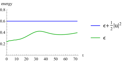
Refer to caption
Figure 5: (Color online) Time evolution of the global energy corresponding to Fig. 4. The total energy (internal energy plus kinetic energy, blue) defined in Eq. (46) remains constant, as expected. The global internal energy (green) can vary in time.

The global energy corresponding to the simulation in Fig. 4 is visualized in Fig. 5. The total energy defined in Eq. (46) remains indeed constant up to numerical precision, while the internal energy varies in time.
Refer to caption
(a) Bloch vectors at t=0𝑡0t=0
Refer to caption
(b) outline of rzsubscript𝑟𝑧r_{z} at t=0𝑡0t=0
Refer to caption
(c) Bloch vectors at t=4𝑡4t=4
Refer to caption
(d) density matrix convergence
Refer to caption
(e) velocity convergence
Refer to caption
(f) total energy convergence
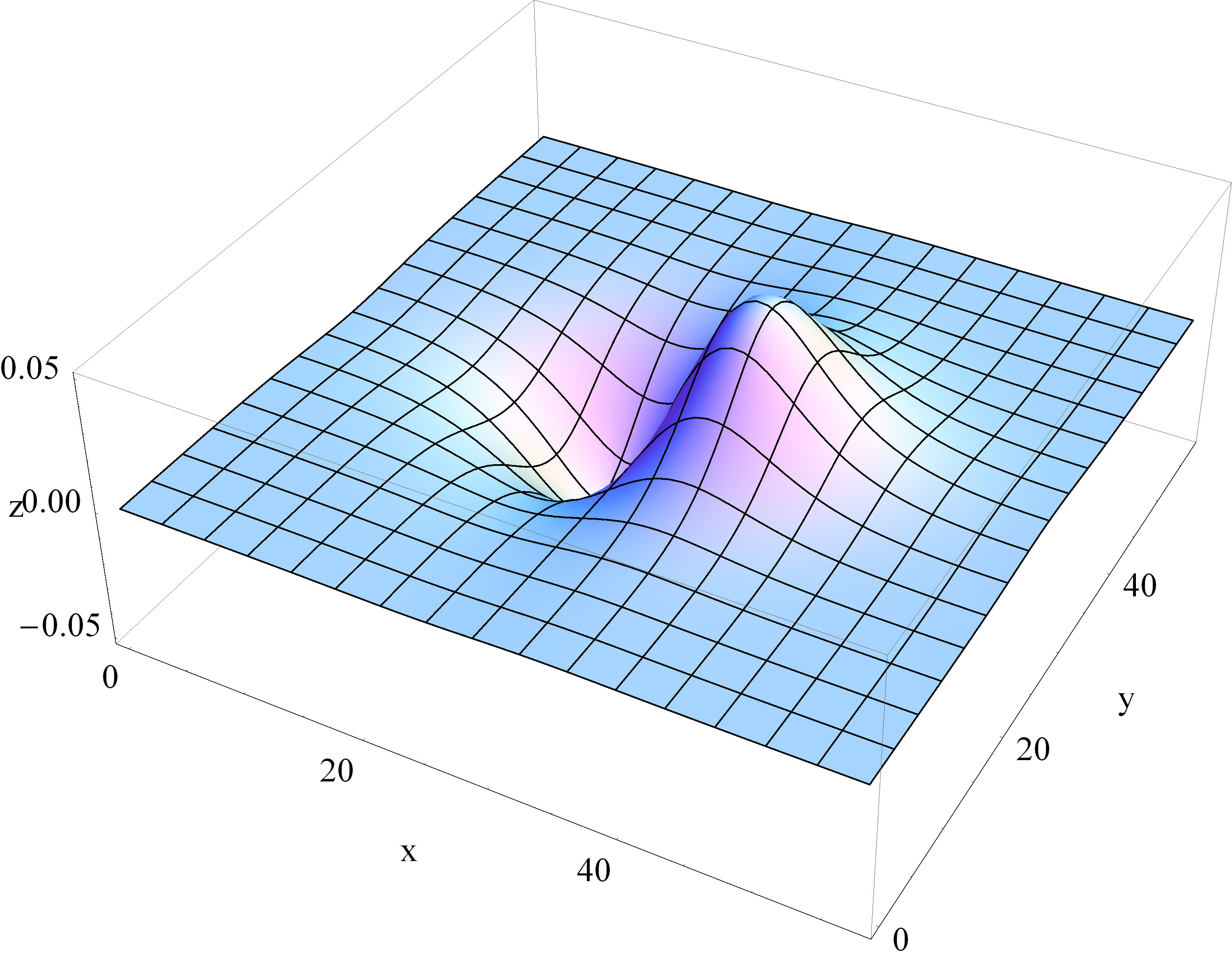
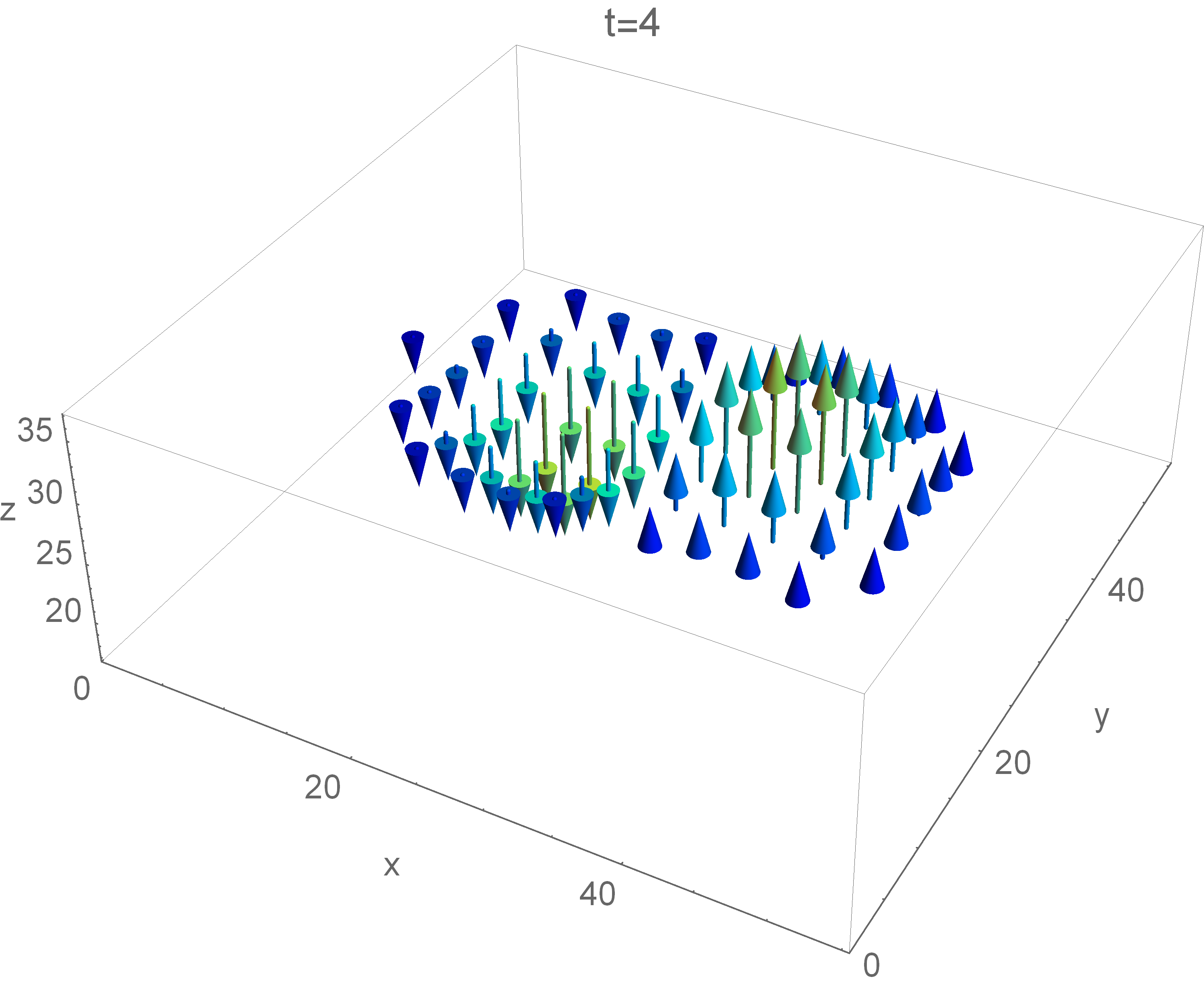
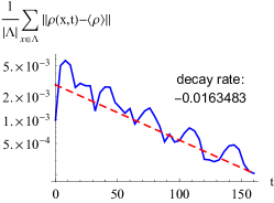
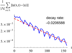
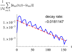
Figure 6: (Color online) Exponential convergence to equilibrium in a 3D simulation. The Bloch vectors of the initial state point along the z𝑧z-axis. (a) shows the vectors within the central z𝑧z-plane, after rescaling them by the factor 350350350 for visual clarity, and (b) the arrow tips as smooth outline. The Bloch vectors tend towards the mean zero vector very rapidly, as illustrated in (c) after 444 time steps only. Color in (a) and (c) encodes the length of the vectors. Bottom row: Quantification of the exponential convergence of the density matrices, velocity and total energy towards their uniform equilibrium values.

Convergence to equilibrium

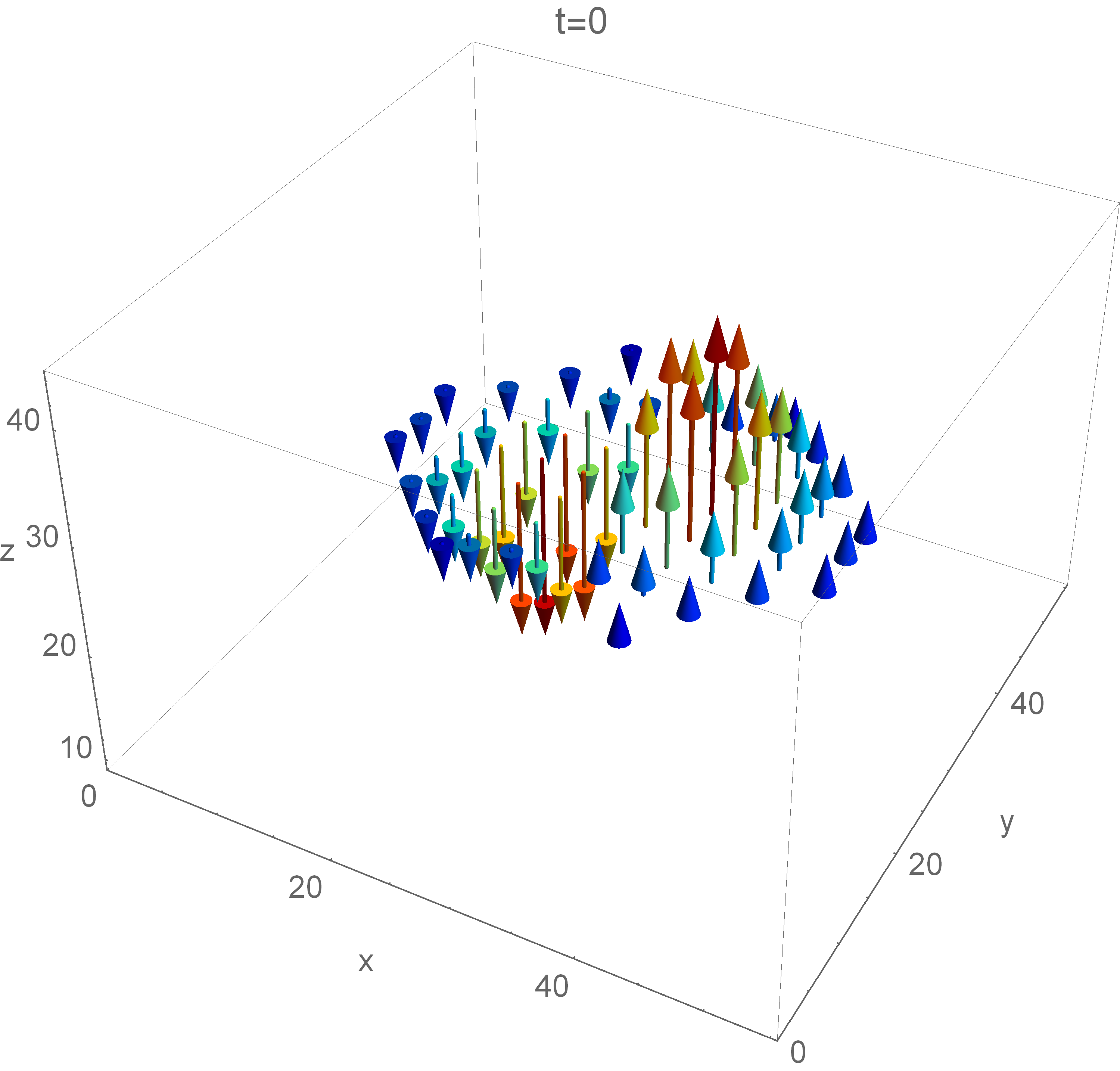
The next example in Fig. 6 illustrates the convergence of the density matrices ρ(𝒙,t)𝜌𝒙𝑡\rho({\boldsymbol{x}},t), velocity 𝒖(𝒙,t)𝒖𝒙𝑡{\boldsymbol{u}}({\boldsymbol{x}},t) and total energy εtot(𝒙,t)subscript𝜀tot𝒙𝑡\varepsilon_{\mathrm{tot}}({\boldsymbol{x}},t) to the constant mean values defined in Eqs. (44) – (46). The simulation domain consists of 32×32×3232323232\times 32\times 32 cells, the relaxation constant was set to τ=10𝜏10\tau=10, and the reference inverse temperature to β0=1subscript𝛽01\beta_{0}=1. The trace of the density matrix is chosen to be uniform, but the z𝑧z-components of the initial Bloch vectors have a dichotomic outline, as shown in Fig. 6a and 6b. Physically, this could correspond to neighboring regions within a solid with opposing (average) electronic spins. The initial velocity points in x𝑥x-direction, with values proportional to the z𝑧z-components of the Bloch vectors. As t𝑡t\to\infty, one expects that the density, velocity and energy become uniform across the simulation domain, and thus converge to their global (equilibrium) average values. Indeed exponential convergence is confirmed numerically in the bottom row of Fig. 6. The oscillatory pattern is likely due to waves which travel in opposite directions and repeatedly collide due to the periodic boundary conditions.

5 Conclusions and outlook

We have developed and implemented a lattice Boltzmann scheme complying with quantum aspects by using Fermi-Dirac equilibrium functions and taking the electronic spin explicitly into account. Still open is a quantification of the error introduced by the BGK approximation as compared to the physical collision operator [1], as well as a calibration of the relaxation time τ𝜏\tau. There are also many desirable features left for future work: in regard of physical applications, an external magnetic field should be included, and various boundary conditions (other than the periodic conditions used in the present study) and additional cell types (like “obstacle” cells appearing in classical LBM) could be incorporated. Concerning the first point, a magnetic field adds a local Vlasov-type commutator

i[μ𝝈𝑩(𝒙,t),W(𝒑,𝒙,t)]𝑖𝜇𝝈𝑩𝒙𝑡𝑊𝒑𝒙𝑡-i\left[\mu\,{\boldsymbol{\sigma}}\cdot{\boldsymbol{B}}({\boldsymbol{x}},t),W({\boldsymbol{p}},{\boldsymbol{x}},t)\right] (47)

to the right side of Eq. (1), where μ𝜇\mu is the magnetic moment, 𝝈=(σx,σy,σz)𝝈subscript𝜎𝑥subscript𝜎𝑦subscript𝜎𝑧{\boldsymbol{\sigma}}=(\sigma_{x},\sigma_{y},\sigma_{z}) the Pauli matrices and 𝑩(𝒙,t)𝑩𝒙𝑡{\boldsymbol{B}}({\boldsymbol{x}},t) the magnetic field. The term (47) can simply be added to the collision operator in the implementation.

Acknowledgments

: I’d like to thank Martin Fürst, Hans Hiptmair and Herbert Spohn for many helpful discussions.

Appendix A Coefficients of the polynomial equilibrium functions

For d=2𝑑2d=2, a solution for the coefficients in Eq. (39) reads

α1subscript𝛼1\displaystyle\alpha_{1} =αfac(3ζ(3)π26β0εFD),absentsubscript𝛼fac3𝜁3superscript𝜋26subscript𝛽0subscript𝜀FD\displaystyle=\alpha_{\text{fac}}\left(3\,\zeta(3)-\frac{\pi^{2}}{6}\beta_{0}\,\varepsilon_{\mathrm{FD}}\right),
α2subscript𝛼2\displaystyle\alpha_{2} =αfac(2log(2)β0εFDπ26),absentsubscript𝛼fac22subscript𝛽0subscript𝜀FDsuperscript𝜋26\displaystyle=\alpha_{\text{fac}}\left(2\log(2)\beta_{0}\,\varepsilon_{\mathrm{FD}}-\frac{\pi^{2}}{6}\right),
α3subscript𝛼3\displaystyle\alpha_{3} =12log(2)π2,absent122superscript𝜋2\displaystyle=\frac{12\log(2)}{\pi^{2}},
α4subscript𝛼4\displaystyle\alpha_{4} =αfaclog(2),α5=αfacπ26,formulae-sequenceabsentsubscript𝛼fac2subscript𝛼5subscript𝛼facsuperscript𝜋26\displaystyle=\alpha_{\text{fac}}\log(2),\quad\alpha_{5}=-\alpha_{\text{fac}}\frac{\pi^{2}}{6},
αfacsubscript𝛼fac\displaystyle\alpha_{\text{fac}} =72log(2)216log(2)ζ(3)π40.60447absent7222162𝜁3superscript𝜋4approaches-limit0.60447\displaystyle=\frac{72\log(2)}{216\log(2)\,\zeta(3)-\pi^{4}}\doteq 0.60447

with εFDsubscript𝜀FD\varepsilon_{\mathrm{FD}} defined in Eq. (20) for d=2𝑑2d=2 and ζ(s)𝜁𝑠\zeta(s) the Riemann zeta function.

Similarly, for dimension d=3𝑑3d=3 one arrives at the solution

α1subscript𝛼1\displaystyle\alpha_{1} =αfac(54(952)ζ(72)(532)ζ(52)β0εFD),absentsubscript𝛼fac54952𝜁72532𝜁52subscript𝛽0subscript𝜀FD\displaystyle=\alpha_{\text{fac}}\left(\frac{5}{4}\left(9-5\sqrt{2}\right)\zeta\!\left(\tfrac{7}{2}\right)-\left(5-3\sqrt{2}\right)\zeta\!\left(\tfrac{5}{2}\right)\beta_{0}\,\varepsilon_{\mathrm{FD}}\right),
α2subscript𝛼2\displaystyle\alpha_{2} =αfac((642)ζ(32)23β0εFD(532)ζ(52)),absentsubscript𝛼fac642𝜁3223subscript𝛽0subscript𝜀FD532𝜁52\displaystyle=\alpha_{\text{fac}}\left(\left(6-4\sqrt{2}\right)\zeta\!\left(\tfrac{3}{2}\right)\tfrac{2}{3}\beta_{0}\,\varepsilon_{\mathrm{FD}}-\left(5-3\sqrt{2}\right)\zeta\!\left(\tfrac{5}{2}\right)\right),
α3subscript𝛼3\displaystyle\alpha_{3} =2ζ(32)(3+2)ζ(52),absent2𝜁3232𝜁52\displaystyle=\frac{2\,\zeta\!\left(\frac{3}{2}\right)}{\left(3+\sqrt{2}\right)\zeta\!\left(\frac{5}{2}\right)},
α4subscript𝛼4\displaystyle\alpha_{4} =αfac(322)ζ(32),α5=αfac(532)ζ(52),formulae-sequenceabsentsubscript𝛼fac322𝜁32subscript𝛼5subscript𝛼fac532𝜁52\displaystyle=\alpha_{\text{fac}}\left(3-2\sqrt{2}\right)\zeta\!\left(\tfrac{3}{2}\right),\quad\alpha_{5}=-\alpha_{\text{fac}}\left(5-3\sqrt{2}\right)\zeta\!\left(\tfrac{5}{2}\right),
αfacsubscript𝛼fac\displaystyle\alpha_{\text{fac}} =4ζ(32)5(952)ζ(32)ζ(72)3(942)ζ(52)21.01062absent4𝜁325952𝜁32𝜁723942𝜁superscript522approaches-limit1.01062\displaystyle=\frac{4\,\zeta\!\left(\frac{3}{2}\right)}{5\left(9-5\sqrt{2}\right)\zeta\!\left(\frac{3}{2}\right)\zeta\!\left(\frac{7}{2}\right)-3\left(9-4\sqrt{2}\right)\zeta\!\left(\frac{5}{2}\right)^{2}}\doteq 1.01062

with εFDsubscript𝜀FD\varepsilon_{\mathrm{FD}} defined in Eq. (20) for d=3𝑑3d=3.

References