Boundary crossover in semi-infinite non-equilibrium growth processes

Abstract

The growth of stochastic interfaces in the vicinity of a boundary and the non-trivial crossover towards the behaviour deep in the bulk is analysed. The causal interactions of the interface with the boundary lead to a roughness larger near to the boundary than deep in the bulk. This is exemplified in the semi-infinite Edwards-Wilkinson model in one dimension, both from its exact solution and numerical simulations, as well as from simulations on the semi-infinite one-dimensional Kardar-Parisi-Zhang model. The non-stationary scaling of interface heights and widths is analyzed and a universal scaling form for the local height profile is proposed.

Improving the understanding of growing interfaces continues [1] as a widely fascinating topic of statistical physics, with a large variety of novel features still being discovered. When considering the growth of interfaces, the situation most commonly analysed is the one of a spatially infinite substrate. Alternatively, if substrates of a finite size are studied, periodic boundary conditions are used. Then, boundary effects need not be taken into account and the scaling of the interface fluctuation can be described in terms of the standard Family-Vicsek (FV) [2] description.

Starting from the height $h(t,x)$, the usual definition of the interface roughness, across the system, is [1]

$$w_{{\rm exp},L}^{2}(t):={\left\langle{\,\overline{\left[h(t,x)-\overline{h(t,x)}\right]^{2}}}\,\right\rangle}={\left\langle\overline{h^{2}(t,x)}\right\rangle}-\left\langle\overline{h(t,x)}^{\>2}\right\rangle,$$ (1)

where $\overline{X}=\overline{X}(t)=L^{-1}\int_{L}\!{\rm d}x\,X(t,x)$ is the spatial average in a system of total spatial size $L$. The ensemble average (over the random noise and/or over all possible realisations) is denoted by $\langle X(t,x)\rangle$. A very commonly studied situation is a finite system of linear size $L$ with periodic boundary conditions. Then, the FV scaling form is [2]

$$\!w_{{\rm exp},L}(t)=t^{\beta}f\left(Lt^{-1/z}\right)\>,\>f(u)\sim\left\{\begin{array}[]{ll}u^{\alpha}&\mbox{\rm; if $u\ll 1$}\\ \mbox{\rm const}&\mbox{\rm; if $u\gg 1$}\end{array}\right.$$ (2)

with the growth exponent $\beta=\alpha/z$. Recently, clear experimental examples with exponents of the Kardar-Parisi-Zhang universaliy class (see below) have been found in turbulent liquid crystals [3] and growing cancer cells [4]. If one furthermore uses a spatially translation-invariant initial condition (e.g. a flat initial surface), then both the average surface profile $\langle h(t,x)\rangle$ and its local width, which we define as

$$w^{2}(t,x):=\left\langle\left[h(t,x)-\left\langle h(t,x)\right\rangle\right]^{2}\right\rangle=\left\langle h^{2}(t,x)\right\rangle-\left\langle h(t,x)\right\rangle^{2},$$ (3)

are space-translation-invariant, hence independent of the location $x$. Then, the width $w^{2}(t,x)\to w_{L}^{2}(t):=\overline{w^{2}(t,x)}=\overline{\langle h(t,x)^{2}\rangle}-\overline{\langle h(t,x)\rangle^{2}}$ can be formally rewritten as a spatial average. At first sight, the two definitions of the bulk roughness, $w_{{\rm exp},L}(t)$ and $w_{L}(t)$, should be different. However, since for a system with spatial translation-invariance one has $\overline{\langle h(t,x)\rangle^{2}}=\left\langle\overline{h(t,x)}\right\rangle^{2}$, they are identical, viz. $w_{{\rm exp},L}^{2}(t)=w_{L}^{2}(t)$, and the explicit average over space in the definition of $w_{L}^{2}(t)$ merely serves to reduce stochastic noise.

 

Figure 1: Schematic noise-averaged interface $\langle h(t,x)\rangle$ (dashed line) and the actual fluctuations around it (full line), in the presence of a boundary at $x=0$.

Here, we are interested in how a boundary in the substrate may affect the properties of the interface. For a system on the half-line $x\geq 0$ with a boundary at $x=0$, space-translation-invariance is broken and both $\langle h(t,x)\rangle$ and $w(t,x)$ depend on the distance $x$ from the boundary, see figure 1. Still, one expects that deep in the bulk $x\gg 1$, the width $w(t,x)$ should converge towards the bulk roughness $w^{2}(t,x)\stackrel{{\scriptstyle x\to\infty}}{{\rightarrow}}w_{\infty}^{2}(t)=w_{{\rm exp},\infty}^{2}(t)$. For finite values of $x$, however, the precise properties of the width $w(t,x)$ will depend on the precise boundary conditions not contained in global quantities such as $w_{L}(t)$ and $w_{{\rm exp},L}(t)$. We shall use (3) to measure the fluctuations of the interface around its position-dependent, ensemble-average value $\left\langle h(t,x)\right\rangle$. This question has since long ago been studied in the past, see [5, 6]. These studies usually begin by prescribing some fixed boundary conditions and then proceed to analyse the position-dependent interface, often through the height profile. In this work, we start from the situation where particles are deposited on a bounded substrate and first ask how the deposition rules become modified in the vicinity of the boundary as compared to deep in the bulk. Generically, bulk models of particle-deposition select first a site on which one attempt to deposit a particle, often followed by a slight redistribution of the particle in the vicinity of the initially selected site, where the details of these rules lead to the numerous recognised universality classes [1, 7, 8]. If one conceives of the boundary as a hard wall which the particles cannot penetrate, those particles which would have to leave the system are kept on the boundary site. Restricting this study for simplicity to a semi-infinite system in $d=1$ space dimensions, this suggests the boundary condition $H_{0}(t)\geq H_{1}(t)$, where $H_{i}(t)$ is the local height on the site $i\geq 0$ such that the boundary occurs at $i=0$.

In contrast to earlier studies [5, 6], it turns out that a continuum description of the interface requires a careful re-formulation of the known bulk models such that the height $h(t,x)$ near to the boundary must be determined self-consistently (throughout, we shall work in the frame moving with the mean interface velocity). Technically, this can be achieved by performing a Kramers-Moyal expansion on the master equation which describes the lattice model defined above. The calculations are rather lengthy and will be reported in detail elsewhere. In the continuum limit, this leads to a non-stationary height profile $\langle h(t,x)\rangle=t^{1/\gamma}\Phi(x^{z}t^{-1})$, with the new scaling relation $\gamma=z/(z-1)$, although stationarity is kept deep in the bulk, where $x\to\infty$ and $\Phi(\infty)=0$. Unexpected behaviour is also found for the width profile $w(t,x)$, see below.

Another motivation of this work comes from the empirical observation that FV-scaling must be generalised in that global and local fluctuations with different values of $\beta$ are to be distinguished [9]. Furthermore, the experimentally measured values of $\beta$ [10, 11, 12, 13, 14, 15, 16] are larger than those expected in many simple model systems [1, 7, 8]. In certain cases, these enhanced values of $\beta$ are experimentally observed together with a grainy, faceted morphology of the interfaces [10, 11, 12, 16] and furthermore, a cross-over in the effective value of $\beta$ from small values at short times to larger values at longer times is seen [10]. While this might suggest that some new exponent should be introduced, this is contradicted by renormalization-group (RG) arguments in bulk systems without disorder or long-range interactions [17].

We study the influence of a substrate boundary on a growing interface by analysing the simplest case of a single boundary in a semi-infinite system, with the condition $H_{0}(t)\geq H_{1}(t)$. It is left for future work to elucidate any possible direct relevance for anomalous roughening. First, we shall study the semi-infinite $1d$ Edwards-Wilkinson (EW) model [18], whose bulk behaviour is well-understood from an exact solution. We shall write down a physically correct Langevin equation in semi-infinite space which includes this new kind of boundary contribution. Its explicit exact solution, of both the height profile as well as the site-dependent interface width, will be seen to be in agreement with a large-scale Monte Carlo (MC) simulations. It turns out that there exists a surprisingly large intermediate range of times where the model crosses over to a new fixed point, with an effective and non-trivial surface growth exponent $\beta_{1,{\rm eff}}>\beta$, which is qualitatively analogous to the experiments cited above. However, at truly large times, typically above the diffusion time, the system converts back to the FV scaling, as expected from the bulk RG [17]. Second, in order to show that these observations do not come from the fact that the Langevin equation of the EW model is linear, we present numerical data for a model in the universality class of the semi-infinite $1d$ Kardar-Parisi-Zhang (KPZ) equation [19]. We find the same qualitative results as for the EW class, with modified exponents. We point out that the time scales needed to see these cross-overs are considerably larger than those studied in existing experiments.

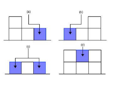
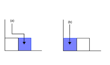
(i)

Figure 2: (i) Family algorithm [20] in the bulk, the particle stays where it falls if the height of the two neighbouring sites is higher (d), or it diffuses to the right or left with the same probability if the neighbours have lower or equal height (c). Finally, the particle diffuses to the right (left) if the neighbour on the left (right) has higher height, see (a) and (b) respectively. (ii) Modification of the Family algorithm on the boundary, the particle diffuses to the right (a) if the height of the neighbour on the right is lower or equal, and stays where it falls otherwise (b).

Edwards-Wilkinson model. In the following we study a microscopic process which should reproduce the $1d$ semi-infinite EW equation, see figure 2(i). A particle incident on a site $i$ of a linear substrate of size $L$ remains there only if its height $H_{i}$ is less or equal to the heights of its two nearest neighbours. If only one nearest-neighbour site has a lower height, deposition is onto that site, but if both nearest-neighbour heights are lower than that of the original site, the deposition site is chosen randomly between the two lower sites with the same probability. In MC simulations, we have taken $L=10^{4}$ and all the data have been averaged over $2\cdot 10^{4}$ samples. This microscopic process [20] associated with periodic boundary condition is known to belong to the EW universality class. We modified the process at the boundary, see figure 2(ii), by imposing that the height of the first site must be higher than the one on the second site, in order to simulate an infinite potential at the origin. This apparently rather weak boundary condition will be seen to lead to significantly new and robust behaviour near to the boundary.

A continuum Langevin equation can be found starting from a master equation for the microscopic process [21, 22]. However these methods may suffer from several problems, like the incomplete determination of the parameters and divergence in the continuum limit when the elementary space step is taken to zero. A Kramers-Moyal expansion on the master equation of the discrete model illustrated in figure 2 leads in the continuum limit to the Langevin equation, defined in the half-space $x\geq 0$

$$\left(\partial_{t}-\nu\partial_{x}^{2}\right)h(t,x)-\eta(t,x)=\nu\left(\kappa_{1}+\kappa_{2}h_{1}(t)\right)\delta(x).$$ (4)

This holds in a co-moving frame with the average interface deep in the bulk (such that $\langle h(t,\infty)\rangle=0$). Furthermore, $\nu$ is the diffusion constant, $\kappa_{1}$ can be considered as an external source at the origin and one defines $h_{1}(t):=\left.\partial_{x}h(t,x)\right|_{x=0}$. Indeed, taking the noise average of (4) and performing a space integration over the semi-infinite chain, we find that $\nu^{-1}\partial_{t}\int_{0}^{\infty}h(t,x){\rm d}x=\kappa_{1}+(\kappa_{2}-1)h_{1}(t)$. We take $\kappa_{2}=1$ since this corresponds to the simplest condition of a constant boundary current $\nu\kappa_{1}\delta(x)$. The centered Gaussian noise has the variance $\left\langle\eta(t,x)\eta(t^{\prime},x^{\prime})\right\rangle=2\nu T\delta(t-t^{\prime})\delta(x-x^{\prime})$, where $T$ is an effective temperature. Parameters $\nu$, $\kappa_{1}$, and $T$ are material-dependent constants and initially, the interface is flat $h(0,x)=0$. With respect to the well-known description of the bulk behaviour [18], the new properties come from the boundary terms on the r.h.s. of eq. (4). In contrast to earlier studies [5], the local slope $h_{1}(t)$ is not a priori given, but must be found self-consistently. In what follows, we choose units such that $\nu=1$. A spatial Laplace transformation leads to

$$h(t,x)\!=\!\frac{1}{4\sqrt{\pi}}\!\int_{{x^{2}}/{4t}}^{\infty}\!\!\frac{{\rm d}v\,{\rm e}^{-v}}{v^{3/2}}\left[x\kappa_{1}+2vh_{0}\left(t-\frac{x^{2}}{4v}\right)\right]+\zeta(t,x),$$ (5)

$$\zeta(t,x)=\int_{0}^{t}\frac{{\rm d}\tau}{\sqrt{4\pi(t-\tau)}}\int_{0}^{\infty}{\rm d}x^{\prime}\eta(\tau,x^{\prime}){\rm e}^{-(x-x^{\prime})^{2}/4(t-\tau)},$$

where $h_{0}(t):=h(t,0)$. The modified noise $\zeta$ is related to noise $\eta$ in terms of its Laplace transform $\overline{\zeta}(t,p):=\int_{0}^{\infty}\!{\rm d}x\>{\rm e}^{-px}\zeta(t,x)=\int_{0}^{t}\!{\rm d}\tau\>{\rm e}^{p^{2}(t-\tau)}\overline{\eta}(\tau,p)$. It remains to determine the function $h_{0}(t)$ self-consistently. Expanding eq. (5) to the first non-trivial order in $x$, we obtain by identification $h_{0}(t)=2\left[\kappa_{1}\pi^{-1/2}\sqrt{t}+\zeta(t,0)\right]$. Introducing the scaling variable $\lambda:=x^{2}/4t$, the height profile and height fluctuation can be cast into the scaling form

$$\!\!\!\!\langle h(t,x)\rangle=\sqrt{t}\,\Phi(\lambda)=\sqrt{t}\,\frac{2\kappa_{1}}{\pi}\left[{\rm e}^{-\lambda}-\sqrt{\pi\lambda\,}\,{\rm erfc\,}\sqrt{\lambda}\right],$$ (6)

$$\!\!\!\!h(t,x)-\langle h(t,x)\rangle=\int_{\lambda}^{\infty}\!\!\frac{{\rm e}^{-v}{\rm d}v}{\sqrt{\pi v}}\>\zeta\left(t-\frac{\lambda t}{v},0\right)+\zeta\left(t,x\right).$$

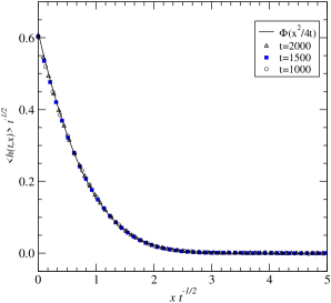
(a)

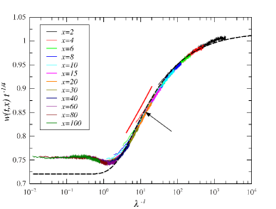
(b)

Figure 3: (a) Mean height profile $\langle h(t,x)\rangle$ in the semi-infinite EW model, and comparison with MC simulations. The full curve gives the scaling function in the first line of eq. (6). (b) Comparison between MC simulations and theoretical prediction for the scaling function $\Phi_{w}(\lambda)$ (dashed black lines, rescaled by a global factor), in the semi-infinite EW model. The scaling variable $\lambda^{-1}=4tx^{-2}$. The arrow indicates the location of the turning point and the slope of the straight line has the value $0.07$.

This scaling form implies the absence of a stationary height profile, in contrast to earlier results [5], although deep in the bulk the profile remains stationary. This is a consequence of the boundary condition $H_{0}(t)\geq H_{1}(t)$. Note that very close to the boundary, the average height $h_{0}(t)\sim\sqrt{t}$ grows monotonically with $t$ such that the interface grows much faster near the boundary than in the bulk. If we had made a scaling ansatz in the noise-averaged version of eq. (4), only the boundary terms as specified in eq. (4) can reproduce $h_{0}(t)$ correctly. On the other hand, for $x\to\infty$, the profile decays as $\left\langle h(t,x)\right\rangle\sim x^{-2}{\rm e}^{-\lambda}$ towards its value deep in the bulk. In Fig 3(a), the mean profile eq. (6) is shown to agree perfectly with direct MC simulations. This confirms the correctness of the Langevin equation eq. (4). A good fit between MC simulations and theoretical predictions is achieved with $\nu=0.79$ and $\kappa_{1}=0.075$, both for the mean profile and width.

Next, we turn to the space-dependent roughness of that interface. In Fig 4, the time-dependence of the interface width, as defined in eq. (3), is displayed for several distances $x$ from the boundary. At small times, one has $w\sim t^{1/4}$ (as expected deep inside the bulk [18, 1]) which at larger times crosses over towards $w\sim t^{\beta_{1,{\rm eff}}}$ with an effective exponent which has a greater, non-trivial value $\beta_{1,{\rm eff}}\approx 0.32$. The scaling $\sim x^{2}$ of the cross-over time-scale suggests that this cross-over occurs, at a fixed distance $x$, when causal interactions with the boundary via diffusive transport occur. This is analogous to the experimentally observed cross-over to anomalous scaling [10, Fig.1]. Can one take this as evidence in favor of a new ‘surface growth exponent’ $\beta_{1}\neq\beta$, distinct from the bulk growth exponent $\beta$ ? In what follows, we shall show, in spite of the suggestive data, that the interpretation of data as in figure 4 is more subtle.

 

Figure 4: Time evolution of the local interface width $w(t,x)$, for several distances $x$ from the boundary, in the semi-infinite EW model. A crossover between two regimes is clearly visible when time is comparable to the diffusion time.

In order to understand this observation, we now compute the width analytically, using the second line of eq. (6). One has $w^{2}(t,x)=W_{1}+W_{2}+W_{3}$, where, after some computation,

$$W_{1} = \frac{1}{\pi}\int\!\!\int_{\lambda}^{\infty}\!\!\!\!\frac{{\rm d}v\,{\rm d}v^{\prime}}{\sqrt{vv^{\prime}}\,{\rm e}^{v+v^{\prime}}}\left\langle\zeta\left(t-\frac{\lambda t}{v},0\right)\zeta\left(t-\frac{\lambda t}{v^{\prime}},0\right)\right\rangle,$$

$$W_{2} = \frac{2}{\sqrt{\pi}}\int_{\lambda}^{\infty}\frac{{\rm d}v}{\sqrt{v}\,{\rm e}^{v}}\left\langle\zeta\left(t-\frac{\lambda t}{v},0\right)\zeta\left(t,x\right)\right\rangle,$$ (7)

$$W_{3} = \left\langle\zeta^{2}\left(t,x\right)\right\rangle=\frac{T\sqrt{t}}{\sqrt{8\pi}}\int_{0}^{t}\!\frac{{\rm d}\tau}{\sqrt{\tau}}\left(1+{\rm erf\,}\sqrt{\frac{2\lambda}{\tau}}\right).$$

It is easy to see that all three terms can be cast into a scaling form $W_{i}=T\sqrt{t}\,{\cal W}_{i}(\lambda)$. ${\cal W}_{3}$ can be evaluated exactly: $\sqrt{2\pi}{\cal W}_{3}=1+{\rm erf\,}\sqrt{2\lambda}+\pi^{-1/2}(2\lambda)^{1/2}\Gamma(0,2\lambda)$, where $\Gamma(s,x)$ is an incomplete gamma function. The other integrals can be partially expressed using special functions, and the behavior near the boundary can be extracted from the series expansion $\lambda\to 0$. We find

$${\cal W}_{1} = \frac{1}{\sqrt{2\pi}}+\Big{(}\gamma+\ln(2)-2+\ln(\lambda)\Big{)}\frac{\sqrt{\lambda}}{\pi}+O(\lambda^{3/2}),$$

$${\cal W}_{2} = \frac{2}{\sqrt{2\pi}}-2\sqrt{\lambda}+\frac{\pi}{2}\lambda+O(\lambda^{2}),$$ (8)

$${\cal W}_{3} = \frac{1}{\sqrt{2\pi}}-\Big{(}\gamma+\ln(2)-2+\ln(\lambda)\Big{)}\frac{\sqrt{\lambda}}{\pi}+O(\lambda^{3/2}).$$

The sum of all these contributions gives $w^{2}(t,x)=T\sqrt{t}\left(4/\sqrt{2\pi}-2\sqrt{\lambda}+O(\lambda^{3/2})\right)$ where the logarithmic terms from ${\cal W}_{1}$ and ${\cal W}_{3}$ cancel each other.

In Fig 3(b), the exact scaling function $\Phi_{w}(\lambda):=w(t,x)t^{-1/4}$ is compared with numerical data for a system of size $L=10^{4}$. Clearly, for large $x$ and not too large $t$, the scaling function is horizontal, which reproduces the expected bulk behaviour $w_{\rm bulk}\sim t^{1/4}$. However, when the scaling variable $\lambda^{-1}=4tx^{-2}$ is increased, the system’s behaviour changes such that the interface at the boundary is rougher than deep in the bulk, as it is exemplified in Fig. 3(b) when $\lambda$ is small. For moderate values of $\lambda$, the scaling function becomes an effective power-law and its slope in Fig 3(b) can be used to define an effective exponent, here of value $\approx 0.07$. This reproduces the effective growth exponent $\beta_{1,{\rm eff}}=\beta+0.07\simeq 0.32$ observed in Fig 4. Remarkably, but certainly in qualitative agreement with RG predictions [17], the scaling function does not increase unboundedly as a function of $\lambda^{-1}$, but rather undergoes a turning point before it saturates, for sites very close to the boundary (where $\lambda\to 0$), such that one recovers the scaling $w\sim t^{1/4}$, with a modified amplitude, however. The Langevin equation with boundary terms, eq. (4), captures completely the change towards the complex behaviour at intermediate values of $\lambda$ and the saturation in the $\lambda\to 0$ limit, but does not yet contain sufficient detail to follow in complete precision the passage from the deep bulk behaviour towards the intermediate regime. In any case, the interface growth as described by the semi-infinite EW model is not described by a new surface exponent but rather by an intermediate regime with an effective anomalous growth in a large time window (between typically $1<\lambda^{-1}<10^{5}$ in Fig. 3(b)), before the standard FV scaling eq. (2) with $\beta=\frac{1}{4}$ is recovered but with a higher amplitude.

Kardar-Parisi-Zhang model. The simplest non-linear growth model, the paradigmatic $1d$ KPZ equation [19]

$$\left(\partial_{t}-\nu\partial_{x}^{2}\right)h(t,x)=\frac{\mu}{2}\left[\partial_{x}h(t,x)\right]^{2}+\eta(t,x),$$

is known to describe a wide range of phenomena [7, 8, 1] and admits the exact critical exponents $z=3/2$, $\beta=1/3$ and $\alpha=1/2$. The $1d$ KPZ equation is also known to be exactly solvable [24, 26, 25] and recently, an extension to a semi-infinite chain has been studied [27]. Here, we report results of MC simulations, based on the RSOS model [28, 29] and scaling arguments. The RSOS process uses a integer height variable $H_{i}(t)\geq 0$ attached to the sites $i=1,\ldots,L$ of a linear chain and subject to the constraints $|H_{i}(t)-H_{i\pm 1}(t)|\leq 1$, at all sites $i$. It is well-known that this process belongs to the KPZ universality class and a continuum derivation of the KPZ equation can be also done as in the EW case [30].

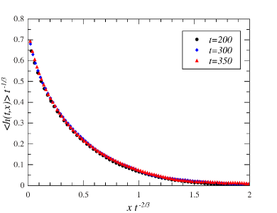
(a)

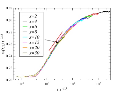
(b)

Figure 5: (a) Height profile $\langle h(t,x)\rangle$ in the semi-infinite RSOS process, showing the scaling form (10), with $z=\frac{3}{2}$ and $\gamma=3$. (b) Time evolution of the local interface width $w(t,x)$, for several distances $x$ from the boundary, in the semi-infinite RSOS model. The arrow indicates the location of the turning point and the slope of the straight line has the value $0.03$.

We now introduce a boundary in the RSOS lattice model, with modified rules in order to simulate a wall, see fig. 2(ii). To this end, we impose $H_{0}(t)\geq H_{1}(t)$ such that the RSOS condition is always satisfied on the left side of the wall, and a particle is deposited on site $i=1$ if the RSOS condition $|H_{1}(t)-H_{2}(t)|\leq 1$ is fulfilled on the right side. In our MC simulations, $L=10^{3}$ and all the data have been averaged over $7\cdot 10^{5}$ samples. The scaling approach is based on the phenomenological boundary-KPZ equation in the half-space

$$\left(\partial_{t}-\nu\partial_{x}^{2}\right)h(t,x)-\frac{\mu}{2}(\partial_{x}h(t,x))^{2}-\eta(t,x)=\nu\left(\kappa_{1}+h_{1}(t)\right)\delta(x).$$ (9)

In general, one expects a scaling of the profile

$$\langle h(t,x)\rangle=t^{1/\gamma}\,\Psi(xt^{-1/z}).$$ (10)

In the linear case $\mu=0$, the above exact EW-solution (6) gives $\gamma=z=2$. Using the scaling form (10) in eq. (9), and assuming a mean-field approximation $\langle(\partial_{x}h(t,x))^{2}\rangle\approx(\partial_{x}\langle h(t,x)\rangle)^{2}$, one may follow [1] and argue that that the nonlinear part should dominate over the diffusion part. Then, we find (the second of these two equations holds true only for $\mu\neq 0$)

$$\frac{1}{z}+\frac{1}{\gamma}=1\;\;,\;\;\frac{2}{z}-\frac{1}{\gamma}=1.$$ (11)

For the KPZ class, this implies $z=3/2$ [19] and $\gamma=3$ . In Fig 5(a), the scaling of the profile of the boundary RSOS model is shown. The predicted exponents lead to a clear data collapse, and the shape is qualitatively similar to the one of the EW-class in Fig 4. The first relation (11) should be correct for any non-linearity describing a boundary growth process because it depends only of the r.h.s. of eq. (9). Hence

$$\gamma=\frac{z}{z-1}=\frac{\alpha}{\alpha-\beta},$$ (12)

should be an universal relation for any $1d$ growth process in presence of a wall . Turning to the local width, our MC simulations give again a site-dependent behaviour, with a crossover to an effective exponent $\beta_{1,\rm{eff}}\approx 0.35$, larger than the bulk exponent $\beta\approx 0.32$ . The scaling form $w(t,x)t^{-\beta}$ shown in Fig 5(b) displays the same qualitative features as seen before in the EW model. This exemplifies that effective anomalous growth behaviour may appear in non-linear (but non-disordered and local) growth processes.

In summary, in several semi-infinite lattice models of interface growth, the simple boundary condition $H_{0}(t)\geq H_{1}(t)$ on the heights on the two sites nearest to the boundary not only leads to non-constant and non-stationary height profiles but also to site-dependent roughness profiles. There exists a large range of times where effective growth exponents $\beta$ with values clearly larger than in deep in the bulk can be identified, in qualitative analogy with known experiments on growing interfaces [10, 11, 12, 13, 14, 15, 16]. However, since we have concentrated on models defined in the simple geometry of a semi-infinite line with a single boundary, a quantitative comparison with the experiments, carried out on faceted growing surfaces with many interacting interfaces, may be premature. For non-disordered models with local interactions, the truly asymptotic growth exponents return to the simple bulk values, as predicted by the RG [17]. The unexpectedly complex behaviour at intermediate times is only seen if appropriate boundary terms are included in the Langevin equation describing the growth process. Our results were obtained through the exact solution of the semi-infinite EW class and through extensive MC simulations of both profiles and widths in the EW and KPZ models. A scaling relation (12) for the surface profile exponent $\gamma$ was proposed and is in agreement with all presently known model results.
 
This work was partly supported by the Collège Doctoral franco-allemand Nancy-Leipzig-Coventry (Systèmes complexes à l’équilibre et hors-d’équilibre) of UFA-DFH.

References

- [1] A.L. Barabási and H.E. Stanley, Fractal concepts in surface growth, Cambridge University Press (1995).
- [2] F. Family and T. Vicsek, J. Phys. A18, L75 (1985).
- [3] K.A. Takeuchi, M. Sano, T. Sasamoto and H. Spohn, Sci. Reports 1:34 (2011) [arxiv:1108.2118]; K.A. Takeuchi and M. Sano, Phys. Rev. Lett. 104, 230601 (2010) [arxiv:1001.5121].
- [4] M.A.C. Huergo, M.A. Pasquale, P.H. González, A.E. Bolzán and A.J. Arvia, Phys. Rev. E85, 011918 (2012).
- [5] D.E. Wolf and L.-H. Tang, Phys. Rev. Lett. 65, 1592 (1990)
- [6] J. Krug, Phys. Rev. Lett. 67, 1882 (1991); H.K. Janssen and K. Oerding, Phys. Rev. E53, 4544 (1996); J.S. Hager, J. Krug, V. Popkov and G.M. Schütz, Phys. Rev. E63, 056110 (2001).
- [7] T. Halpin-Healy and Y.-C. Zhang, Phys. Rep. 254, 215 (1995).
- [8] J. Krug, Adv. Phys. 46, 139 (1997).
- [9] J.J. Ramasco, J.M. López and M.A. Rodríguez, Phys. Rev. Lett. 84, 2199 (2000) [cond-mat/0001111]; Europhys. Lett. 76, 554 (2006) [cond-mat/0603679].
- [10] F.S. Nascimento, S.C. Ferreira and S.O. Ferreira, Europhys. Lett. 94, 68002 (2011) [arxiv:1101.1493].
- [11] S. Yim and T.S. Jones, Appl. Phys. Lett. 94, 021911 (2009).
- [12] A.C. Dürr et al., Phys. Rev. Lett. 90, 016104 (2003).
- [13] A.S. Mata, S.C. Ferreira, I.R.B. Ribeiro and S.O. Ferreira, Phys. Rev. B78, 115305 (2008) [arxiv:1101.1167].
- [14] H. Gong and S. Yim, Bull. Korean Chem. Soc. 32, 2237 (2011).
- [15] J. Kim, N. Lim, C.R. Park and S. Yim, Surf. Science 604, 1143 (2010).
- [16] P. Cordoba-Torres, T.J. Mesquita, I.N. Bastos and R.P. Nogueira, Phys. Rev. Lett. 102, 055504 (2009).
- [17] J.M. López, M. Castro and R. Gallego, Phys. Rev. Lett. 94, 166103 (2005) [cond-mat/0503703].
- [18] S.F. Edwards and D.R. Wilkinson, Proc. Roy. Soc. A381, 17 (1982).
- [19] M. Kardar, G. Parisi and Y.-C. Zhang, Phys. Rev. Lett. 56, 889 (1986).
- [20] F. Family, J. Phys. A19, L441 (1986).
- [21] D.D. Vvedensky, A. Zangwill, C.N. Luse, and M.R. Wilby, Phys. Rev. E48, 852 (1993).
- [22] A.L.-S. Chua, C.A. Haselwandter, C. Baggio, and D.D. Vvedensky, Phys. Rev. E72, 051103 (2005).
- [23] John Crank, The mathematics of diffusion, Oxford University Press, (Oxford 1975).
- [24] P. Calabrese and P. Le Doussal, Phys. Rev. Lett. 106, 250603 (2011) [arxiv:1104.1993].
- [25] T. Sasamoto and H. Spohn, J. Stat. Mech. P11013 (2010) [arxiv:1010.2691].
- [26] T. Sasamoto and H. Spohn, Phys. Rev. Lett. 104, 230602 (2010) [arxiv:1002.1883].
- [27] T. Gueudré and P. Le Doussal, Europhys. Lett. 100, 26006 (2012). [arxiv:1208.5669]
- [28] J.M. Kim and J.M. Kosterlitz, Phys. Rev. Lett. 62, 2289 (1989).
- [29] M. Henkel, J.D. Noh and M. Pleimling, Phys. Rev. E85, 030102(R) (2012). [arxiv:1109.5022]
- [30] K. Park and B. Kahng, Phys. Rev. E51, 796 (1995).