A New Chase-type Soft-decision Decoding Algorithm for Reed-Solomon Codes
Abstract
A new Chase-type soft-decision decoding algorithm for Reed-Solomon codes is proposed, referred to as tree-based Chase-type algorithm. The proposed tree-based Chase-type algorithm takes the set of all vectors as the set of testing patterns, and hence definitely delivers the most-likely codeword provided that the computational resources are allowed. All the testing patterns are arranged in an ordered rooted tree according to the likelihood bounds of the possibly generated codewords, which is an extension of Wu and Pados’ method from binary into -ary linear block codes. While performing the algorithm, the ordered rooted tree is constructed progressively by adding at most two leafs at each trial. The ordered tree naturally induces a sufficient condition for the most-likely codeword. That is, whenever the tree-based Chase-type algorithm exits before a preset maximum number of trials is reached, the output codeword must be the most-likely one. But, in fact, the algorithm can be terminated by setting a discrepancy threshold instead of a maximum number of trials. When the tree-based Chase-type algorithm is combined with Guruswami-Sudan (GS) algorithm, each trial can be implement in an extremely simple way by removing from the gradually updated Gröbner basis one old point and interpolating one new point. Simulation results show that the tree-based Chase-type algorithm performs better than the recently proposed Chase-type algorithm by Bellorado et al with less trials (on average) given that the maximum number of trials is the same.
Index Terms:
Error-correction codes, Chase-type algorithm, flipping patterns, Guruswami-Sudan algorithm, hard-decision deocoding, Reed-Solomon codes, soft-decision decoding.I Introduction
Reed-Solomon (RS) codes are an important class of algebraic codes, which have been widely used in many practical systems, including space and satellite communications, data storage, digital audio/video transmission and file transfer [1]. Even more contemporary codes such as turbo product codes (TPC) [2, 3, 4] can be used with RS codes. The widespread use of RS codes is primarily due to their large error-correction capability, a consequence of their maximum distance separable (MDS) property. Investigating the decoding algorithms for RS codes is important both in practice and in theory. The traditional hard-decision decoding (HDD) algorithms, such as Berlekamp-Massey (BM) [5], Welch-Berlekamp (WB) [6] and Euclidean [7] algorithms, are efficient to find the unique codeword (if exists) within a Hamming sphere of radius less than the half minimum Hamming distance. Hence, their error-correction capability is limited by the half minimum Hamming distance bound. In contrast, Guruswami-Sudan (GS) algorithm [8][9] can enlarge the decoding radius and may output a list of candidate codewords. Hence, GS algorithm can correct errors beyond the half minimum Hamming distance bound. Nevertheless, HDD algorithms do not fully exploit the information provided by the channel output. The Koetter-Vardy (KV) algorithm [10] extended the GS decoder to an algebraic soft-decision (ASD) decoding algorithm by transforming the soft information into the multiplicity matrix that is then taken as input to the GS decoder.
The KV algorithm outperforms the GS algorithm but suffers from high complexity. To reduce the complexity, a progressive list-enlarged algebraic soft-decision decoding algorithm has been proposed in [11][12]. The other class of soft-decision decoding (SDD) algorithms, which are based on using multiple trials of a low-complexity RS decoding algorithm in combination with erasing or flipping a set of symbols or bits in each trial, have renewed the interest of researchers. These algorithms use the soft-information available at the channel output to construct a set of either erasure patterns [13, 14, 15, 16], flipping patterns [17, 18, 19], or patterns combining both [20][21], and then attempt to decode using each pattern. Meanwhile, more related works focus on how to select patterns [22, 23], how to rule out useless patterns [24] and how to identify the maximum-likelihood (ML) codeword [25][26]. Other soft-decision decoding algorithms based on multiple trials can be found in [27, 28, 29]. In [27], re-encoding is performed for each trial, where the generator matrix is adapted based on most reliable positions (MRPs) specified by the ordered statistics. In [28] and [29], a decoding algorithm combined with belief propagation is performed for each trial, where the parity-check matrix is iteratively adapted based on the LRPs.
In this paper, we focus on the Chase-type decoding algorithm. Let be an RS code over the finite field of size with length , dimension , and the minimum Hamming distance , Generally, a Chase-type soft-decision decoding algorithm has three ingredients: 1) a set of flipping patterns where is a vector of length , 2) a hard-decision decoder (HDD), and 3) a stopping criterion. Given these three ingredients, a Chase-type decoding algorithm works as follows. For each , the Chase-type algorithm makes a trial by decoding with the HDD. If the HDD is successful, the output is referred to as a candidate codeword. Once some candidate is found to satisfy the stopping criterion, the algorithm terminates. Otherwise, the algorithm chooses as output the most likely candidate after all flipping patterns in are tested.
The Chase-2 decoding algorithm [17], which is well known for binary codes, finds the LRPs, and then constructs the commonly-used by flipping patterns combinatorially. Obviously, the straightforward generalization of Chase-2 from binary to nonbinary incurs high complexity especially for large and . Later, Wu and Pados [18] proposed an adaptive two-stage algorithm for ML/sub-ML decoding, where in the first stage the flipping patterns in are constructed dynamically according to their ascending lower bound on the soft discrepancy. With this testing order, the ML codeword is expected to appear earlier. This order also provides a sufficient condition to terminate the algorithm before all flipping patterns are tested. However, Wu and Pados did not show explicitly in [18] the way to generate the ordered flipping patterns, especially for nonbinary codes. Next, a low-complexity Chase (LCC) decoding algorithm [19] for RS codes, which can achieve better performance-complexity tradeoff, constructs flipping patterns by first finding LRPs and then restricts only two most likely symbols at each LRP. For the HDD algorithm required in the Chase-type algorithm, one usually chooses a simple HDD algorithm, such as BM algorithm. In contrast, the LCC algorithm implements the GS decoding algorithm (with multiplicity one) for each trial. This algorithm has a clear advantage when two flipping patterns diverge in only one coordinate, in which case backward interpolation architecture [30] and the module basis reduction interpolation technique [31] can be employed to further reduce the decoding complexity. Because of this, even though the set of erasure patterns designed using rate-distortion theory in [16] may slightly outperform the LCC algorithm with the same number of decoding trials, the latter may require lower implementation complexity.
In this paper, we propose to arrange all possible flipping patterns into an ordered rooted tree, which is constructed progressively by adding at most two leafs at each trial. With the aid of the inherent structure of the tree, we devise an efficient algorithm that generates one-by-one upon request flipping patterns according to their soft discrepancy lower bounds. To expedite the decoding, we propose a sufficient condition that generalizes Taiple and Pursley’s condition [32] to prune some unnecessary sub-trees. In addition, when the new algorithm is combined with the GS algorithm, each trial can be implement in an extremely simple way by removing from the gradually updated Gröbner basis one old point and interpolating one new point. Simulation results show that the proposed algorithm performs better than the LCC algorithm [19] with less trials (on average) given that the maximum number of trials is the same. To illustrate the near-optimality of the proposed algorithm in the high signal-to-noise ratio (SNR) region, we also propose a method to simulate performance bounds on the maximum-likelihood decoding (MLD) algorithm.
The rest of this paper is organized as follows. Sec. II defines the ordered rooted tree of flipping patterns and provides a general framework of the tree-based Chase-type algorithm. In Sec. III, the tree-based Chase-type algorithm is combined with the GS algorithm. Numerical results and further discussion are presented in Sec. IV. Sec. V concludes this paper.
II Testing Order of Flipping Patterns
II-A Basics of RS Codes
Let be the finite field of size . A codeword of the RS code can be obtained by evaluating a polynomial of degree less than over distinct points, denoted by . To be precise, the codeword corresponding to a message polynomial is given by
Assume that the codeword c is transmitted through a memoryless channel, resulting in a received vector
The corresponding hard-decision vector is denoted by
where . Here, we are primarily concerned with additive white Gaussian noise (AWGN) channels. In this scenario, a codeword is modulated into a real signal before transmission and the channel transition probability function is replaced by the conditional probability density function.
The error pattern is defined by . A conventional hard-decision decoder (HDD) can be implemented to find the transmitted codeword whenever the Hamming weight is less than or equal to . The HDD is simple, but it usually causes performance degradation. In particular, it even fails to output a valid codeword if z lies at Hamming distance greater than from any codeword. An optimal decoding algorithm (to minimize the word error probability when every codeword is transmitted equal-likely) is the maximum likelihood decoding (MLD) algorithm, which delivers as output the codeword c that maximizes the log-likelihood metric . The MLD algorithm is able to decode beyond errors, however, it is computationally infeasible in general [33]. A Chase-type soft-decision decoding algorithm trades off between the HDD and the MLD by performing the HDD successively on a set of flipping patterns.
II-B Minimal Decomposition of Hypothesized Error Patterns
Similar to [34, Chapter 3], we introduce the following definitions.
Definition 1
Let z be the hard-decision vector. A hypothesized error pattern e is defined as a vector such that is a valid codeword.
Notice that z itself is a hypothesized error pattern since is the all-zero codeword. To each component of the hypothesized error pattern, we assign a soft weight . The soft weight of a hypothesized error pattern e is defined as . The MLD algorithm can be equivalently described as finding one lightest hypothesized error pattern that minimizes .
Since the soft weight of a hypothesized error pattern e is completely determined by its nonzero components, we may simply list all its non-zero components. For clarity, a nonzero component of e is denoted by meaning that an error of value occurs at the -th coordinate, i.e., . For convenience, we call with an atom. In the following, we will define a total order over the set of all atoms. For the purpose of tie-breaking, we define simply a total order over the field as .
Definition 2
We say that if and only if or and or , and .
With this definition, we can arrange all the atoms into a chain (denoted by A and referred to as atom chain) according to the increasing order. That is,
| (1) |
The rank of an atom , denoted by , is defined as its position in the atom chain A.
Definition 3
Let f be a nonzero vector. Its support set is defined as , whose cardinality is the Hamming weight of f. Its lower rank and upper rank are defined as and , respectively.
We assume that and .
Proposition 1
Any nonzero vector f can be represented in a unique way by listing all its nonzero components as
| (2) |
where , and .
Proof:
It is obvious and omitted here. ∎
Proposition 1 states that any nonzero vector can be viewed as a sub-chain of A. In contrast, any sub-chain of A specifies a nonzero vector only when all atoms in the sub-chain have distinct coordinates.
Proposition 2
Any nonzero vector e with can be uniquely decomposed as satisfying that , and .
Proof:
From Proposition 1, we have where . Then this proposition can be verified by defining and . ∎
For a vector f, define . From Proposition 2, any hypothesized error pattern e with can be decomposed as in a unique way such that . This decomposition is referred to as the minimal decomposition111This terminology comes from the fact as shown in Appendix A., where f is referred to as the minimal flipping pattern associated with e. In the case when a hypothesized error pattern e exists with , we define 0 as the minimal flipping pattern associated with e.
For every , when taking as an input vector, the HDD either reports a decoding failure or outputs a unique codeword c. In the latter case, we say that the flipping pattern f generates the hypothesized error pattern . Actually, any hypothesized error pattern can be generated by many flipping patterns (collectively referred to as equivalence class in [35]). Apparently, an efficient algorithm should avoid to test multiple flipping patterns in the same equivalence class. As pointed out in [35][24], we have the following proposition.
Proposition 3
Any hypothesized error pattern can be generated by its associated minimal flipping pattern.
Proof:
It is obvious. ∎
From Proposition 3, in principle, we only need to decode all vectors with the minimal flipping patterns f. Unfortunately, we do not know which flipping patterns are minimal before performing the HDD. Even worse, we do not know whether or not a vector f can generate a hypothesized error pattern before performing the HDD. However, by extending the Proposition 1 in [18], we have the following theorem, which provides a lower bound on the soft weight of the generated error pattern whenever f is a minimal flipping pattern.
Theorem 1
Let f be a nonzero vector that is the minimal flipping pattern to generate a hypothesized error pattern e. Then .
More importantly, the lower bound given in Theorem 1 is computable for any nonzero vector f without performing the HDD since can be calculated using the following greedy algorithm with the help of the atom chain A.
Algorithm 1: Greedy Algorithm for Computing .
-
•
Input: A nonzero vector f.
-
•
Initialization: Set , , and .
-
•
Iterations: While and , do
-
1.
if , let , and .
-
2.
.
-
1.
-
•
Output: If , output . Otherwise, we must have ; in this case, output .
The correctness of the above greedy algorithm can be argued as follows. Let be the sub-chain of A found when the algorithm terminates. This sub-chain must be a vector since no two atoms contained in can have the same coordinate for that each atom is added only when . We only need to consider the case when , which is equivalent to saying that all atoms with rank greater than occupy at least coordinates. In this case, we must have . We then have since and for that begins with and each atom is added only when . The minimality of can be proved by induction on the iterations.
II-C Tree of Flipping Patterns
All flipping patterns are arranged in an ordered rooted tree, denoted by T, as described below.
-
T1.
The root of the tree is , which is located at the 0-th level. For , the -th level of the tree consists of all nonzero vectors with Hamming weight .
-
T2.
A vertex f at the -th level takes as children all vectors from , which are arranged at the -th level from left to right with increasing upper ranks. The root has children. A nonzero vertex f has at most children.
For each vertex f in T, define
| (3) |
Theorem 2
Let f be a vertex. If exist, let be its parent, be one of its children and be one of its right-siblings. We have and .
Proof:
We have since has one more atom than f. We also have since . Therefore, .
For a nonzero vertex f, we have and where . Hence , which implies that . Let such that . If , define , where is an atom contained in ; otherwise, define . In either case, we can verify that and , implying that . Therefore, we have . ∎
Definition 4
A subtree is said to be sufficient for the MLD algorithm if the lightest hypothesized error pattern can be generated by some vertex in .
By this definition, we can see that T is itself sufficient. We can also see that removing all vertexes with Hamming weight greater than does not affect the sufficiency. Generally, we have
Theorem 3
Let be an available hypothesized error pattern and f be a nonzero vertex such that . Then removing the subtree rooted from f does not affect the sufficiency.
Proof:
If exists, let e be a hypothesized error pattern such that . It suffices to prove that e can be generated by some vertex in the remaining subtree. Let h be the minimal flipping pattern associated with e. From Theorem 1, we have . From Theorem 2, h is not contained in the subtree rooted from f and hence has not been removed. ∎
Similar to [18], a total order of all vertexes can be defined as follows.
Definition 5
We say that if and only if or and or , and f is located at the left of h.
Suppose that we have an efficient algorithm that can generate one-by-one upon request all flipping patterns in the following order
| (4) |
Then we can perform a Chase-type algorithm as follows. For , we perform the HDD by taking as the input. If a hypothesized error pattern is found satisfying , then the algorithm terminates. Otherwise, the process continues until a preset maximum number of trials is reached. The structure of the tree T is critical to design such an efficient sorting algorithm. From Theorem 2, we know that and . Therefore, must be either the left-most child of some with or the following (adjacent) right-sibling of some with . In other words, it is not necessary to consider a flipping pattern f before both its parent and its preceding left-sibling are tested. This motivates the following Chase-type algorithm, referred to as tree-based Chase-type algorithm.
Algorithm 2: A General Framework of Tree-based Chase-type Algorithm
-
•
Preprocessing: Find the hard-decision vector z; calculate the soft weights of atoms; construct the atom chain A. Suppose that we have a linked list , which is of size at most and maintained in order during the iterations.
-
•
Initialization: ; ; .
-
•
Iterations: While , do the following.
-
1.
If , output and exit the algorithm;
-
2.
Perform the HDD by taking as input;
-
3.
In the case when the HDD outputs a hypothesized error pattern e such that , set ;
-
4.
Update the linked list by inserting (if exist) the left-most child and the following right-sibling of and removing ;
-
5.
Increment by one.
-
1.
Remarks.
-
•
The vector can be initialized by any hypothesized error pattern (say obtained by the re-encoding approach) other than z. Or, we may leave uninitialized and set initially.
-
•
Obviously, the computational complexity of preprocessing step is . Note that, in each iteration of Algorithm 2, one flipping pattern is removed from and at most two flipping patterns are inserted into . Also note that the size of can be kept as less than or equal to by removing extra tailed flipping patterns. Hence maintaining the linked list requires computational complexity of order at most , which is consistent with [18, Theorem 1]. If the algorithm exits within iterations, the found hypothesized error pattern must be the lightest one.
-
•
The above algorithm is an extension of this process, which is referred to as LB ascending search in [18] and that is the optimal searching order in the sense that the HDD approaches rapidly the ML codeword, i.e., the lightest error pattern. During the iterations, sufficient conditions in [25] or Lemma 1 in [26] for -ary RS codes (see the corrected form in [36]) can also be used to identify the lightest error pattern. The lemma is rephrased as follows.
Theorem 4
If an error pattern satisfies
| (5) |
where , . Then there exists no error pattern which is lighter than .
Proof:
Let e be a hypothesized error pattern. Since any two hypothesized error patterns must have Hamming distance at least , we have . ∎
Note that the bound can be calculated by a greedy algorithm similar to Algorithm 1.
III The Tree-based Chase-type GS Algorithm
From the framework of the tree-based Chase-type algorithm, we see that the flipping pattern at the -th trial diverges from its parent (which has been tested at the -th trial for some ) in one coordinate. This property admits a low-complexity decoding algorithm if GS algorithm is implemented with multiplicity one and initialized Gröbner basis . Let be the -degree of and be the -weighted degree of .
Proposition 4
Let f be a flipping pattern and be the Gröbner basis for the -module . Then can be found from by backward interpolation and forward interpolation.
Proof:
Denote the two polynomials in the Gröbner basis by . Let the right-most atom of f is which is the only atom contained in f but not in . We need to update by removing the point and interpolating the point . This can be done according to the following steps, as shown in [37].
-
•
Use backward interpolation to eliminate the point of :
-
1.
Compute for ; let ; let ;
-
2.
If , then ;
-
3.
and ;
-
1.
-
•
Use forward interpolation (Kötter’s algorithm) to add the point :
-
1.
Compute ; let ; let ;
-
2.
;
-
3.
.
-
1.
To summarize, from , we can obtain efficiently. ∎
The main result of this section is the following tree-based Chase-type GS decoding algorithm for RS codes.
Algorithm 3: Tree-based Chase-type GS Decoding Algorithm for RS Codes
-
•
Preprocessing: Upon on receiving the vector r, find the hard-decision vector z; compute the soft weights of all atoms; construct the atom chain A.
-
•
Initialization:
-
1.
; ; ; ;
-
2.
Input z to the GS algorithm with multiplicity one and initialized Gröbner basis , resulting in ;
-
3.
Factorize the minimal polynomial in . If a message polynomial is found, find , where c is the codeword corresponding to ; if , set and ; if, additionally, , output and exit the algorithm;
-
4.
Insert (the left-most child of f) into and remove 0 from ; set ;
-
5.
Set .
-
1.
-
•
Iterations: While , do the following.
-
1.
Set ; if , output and exit the algorithm;
-
2.
Let be the right-most atom of f. Update by removing the point and interpolating the point ;
-
3.
Factorize the minimal polynomial in . If a message polynomial is found, find , where c is the codeword corresponding to ; if , set and ; if, additionally, , output and exit the algorithm;
-
4.
Insert (if exist) (the left-most child of f) and (the following right-sibling of f) into ; set and ; remove from the linked list ;
-
5.
Increment by one.
-
1.
Remark.
-
•
It is worth pointing out that the factorization step in Algorithm 3 can be implemented in a simple way as shown in [38]. Let be the polynomial to be factorized. If divides , set . If , is a valid message polynomial.
-
•
Note that, to use the backward interpolation techniques in Algorithm 3, besides maintaining the linked list , we have to reserve these interpolation polynomials corresponding to their parents. Since the size of can be kept as less than or equal to by removing extra tailed flipping patterns, maintaining the linked list requires extra reservation at most . By observing the step 2) and 3) in backward and forward interpolation, we can conclude that its complexity is roughly at each iteration.
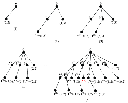
To illustrate clearly the construction of the tree T as well as the tree-based Chase-type GS decoding algorithm, we give below an example.
Example 1
Consider the RS code over with . Let the message polynomial and . Then the codeword . Let r be the received vector from a memoryless channel that specifies the following log-likelihood matrix
where for and .
The tree-based Chase-type GS decoding algorithm with is performed as follows.
Preprocessing: Given the log-likelihood matrix , find the hard-decision vector . Find the soft weights of all atoms, which can be arranged as
where is the soft weight of atom for and . Given , all the atoms can be arranged into the atom chain
Initialization:
-
1.
; ; ; ; ;
-
2.
input to the GS decoder and obtain ;
-
3.
factorize ; since is divisible by , find a valid message polynomial , which generates the codeword ; obtain and ; since , we set and ; since , the algorithm continues;
-
4.
insert (the left-most child of 0) into as shown in Fig. 1-(1) and remove 0 from ; set ; at this step, the linked list with ;
-
5.
set ;
Iterations: While , do
When ,
-
1.
set ; since , the algorithm continues;
-
2.
since the right-most atom of f is , update by removing and interpolating and obtain ;
-
3.
factorize ; since is divisible by , find a valid message polynomial , which generates the codeword ; obtain and compute ; since , we set and ; since , the algorithm continues;
-
4.
insert and into as shown in Fig. 1-(2); set and ; remove from the linked list ; at this step, the linked list , where ;
-
5.
set .
When ,
-
1.
set ; since , the algorithm continues;
-
2.
since the right-most atom of f is , update by removing and interpolating and obtain ;
-
3.
factorize ; since is divisible by , find a valid message polynomial , which generates the codeword ; obtain and ; since , updating and are not required;
-
4.
insert and into as shown in Fig. 1-(3); set and ; remove from the linked list ; at this step, the linked list , where ;
-
5.
set .
When ,
-
1.
set ; since , the algorithm continues;
-
2.
since the right-most atom of f is , update by removing and interpolating and obtain ;
-
3.
factorize ; no candidate codeword is found at this step;
-
4.
insert and into as shown in Fig. 1-(4); set and ; remove from the linked list ; at this step, the linked list , where ;
-
5.
set .
When ,
-
1.
set ; since , the algorithm continues;
-
2.
since the right-most atom of f is , update by removing and interpolating and obtain ;
-
3.
factorize ; since is divisible by , find a valid message polynomial , which generates the codeword ; obtain and ; since , set and ; since , the algorithm continues;
-
4.
insert and into as shown in Fig. 1-(5); set and with ; remove from the linked list ; at this step, the linked list , where ;
-
5.
update .
When ,
-
1.
set ; since , output and exit the algorithm.
IV Numerical Results and Further Discussions
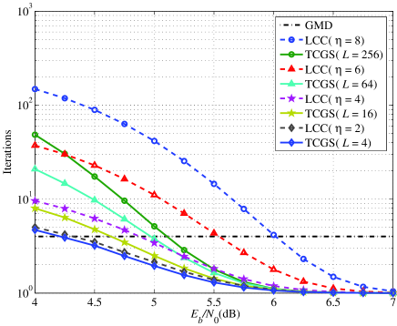
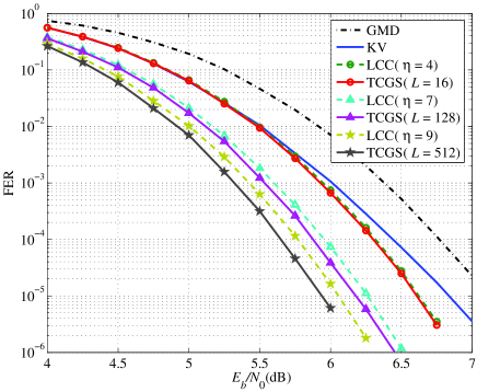
In this section, we compare the proposed tree-based Chase-type GS (TCGS) decoding algorithm with the LCC decoding algorithm [19]. We take the LCC decoding algorithm as a benchmark since the TCGS algorithm is similar to the LCC algorithm with the exception of the set of flipping patterns and the testing orders. In all examples, messages are encoded by RS codes and then transmitted over additive white Gaussian noise (AWGN) channels with binary phase shift keying (BPSK) modulation. The performance is measured by the frame error rate (FER), while the complexity is measured in terms of the average testing numbers. For a fair and reasonable comparison, we assume that these two algorithms perform the same maximum number of trials, that is, . The LCC decoding algorithm takes Theorem 4 as the early stopping criterion, while the TCGS decoding algorithm takes both Theorem 3 and Theorem 4 as the early stopping criteria. Notice that Theorem 3 is one inherent feature of the TCGS algorithm, which does not apply to the LCC algorithm. For reference, the performance of the GMD decoding algorithm and that of the theoretical KV decoding algorithm (with an infinite interpolation multiplicity) are also given.
IV-A Numerical Results
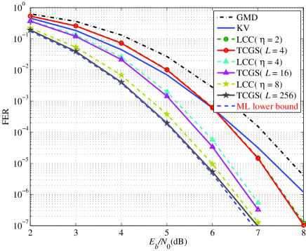
Example 2
Consider the RS code over with . The performance curves are shown in Fig. 2. We can see that the TCGS algorithm performs slightly better than the LCC algorithm. As increases, the gap becomes larger. At FER = , the TCGS algorithm with outperforms the LCC algorithm (with ) and the GMD algorithm by dB and dB, respectively. Also note that, even with small number of trials, the TCGS algorithm can be superior to the KV algorithm.
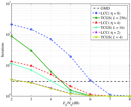
The average iterations are shown in Fig. 3. It can be seen that the average decoding complexity of both the TCGS and the LCC algorithms decreases as the SNR increases. The TCGS algorithm requires less average iterations than the LCC algorithm. Furthermore, the average iterations required for the TCGS algorithm are even less than those for the GMD algorithm when dB.
Example 3
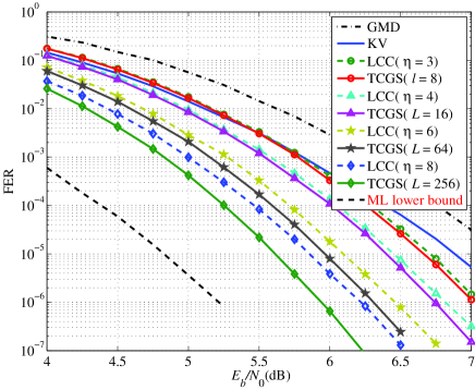
Consider the RS code over with . The performance curves are shown in Fig. 4. We can see that the TCGS algorithm performs slightly better than the LCC algorithm. As increases, the gap becomes larger. At FER = , the TCGS algorithm with outperforms the LCC algorithm (with ) and the GMD algorithm by dB and dB, respectively. Also note that, even with small number of trials, the TCGS algorithm can be superior to the KV algorithm.
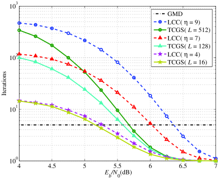
The average iterations are shown in Fig. 5. It can be seen that the average decoding complexity of both the TCGS and the LCC algorithms decreases as the SNR increases. The TCGS algorithm requires less average iterations than the LCC algorithm. Furthermore, the average iterations required for the TCGS algorithm are even less than those for the GMD algorithm when dB.
Example 4
Consider the RS code over with . The performance curves are shown in Fig. 6. We can see that the TCGS algorithm performs slightly better than the LCC algorithm. As increases, the gap becomes larger. At FER = , the TCGS algorithm with outperforms the LCC algorithm (with ) and the GMD algorithm by dB and dB, respectively. Also note that, even with small number of trials, the TCGS algorithm can be superior to the KV algorithm.
The average iterations are shown in Fig. 7. It can be seen that the average decoding complexity of both the TCGS and the LCC algorithms decreases as the SNR increases. The TCGS algorithm requires less average iterations than the LCC algorithm. Furthermore, the average iterations required for the TCGS algorithm are even less than those for the GMD algorithm when dB.
IV-B Complexity Analysis
In summary, we have compared by simulation the tree-based Chase-type GS (TCGS) decoding algorithm with the LCC decoding algorithm, showing that the TCGS algorithm has a better performance and requires less trials for a given maximum testing number. We will not argue that the proposed algorithm has lower complexity since it is difficult to make such a comparison. The difficulty lies in that, although the interpolation process in the finite field is simple, the proposed algorithm requires pre-processing and evaluating the lower bound for each flipping pattern in the real field. As mentioned above, the computation of preprocessing step is , and to maintain the linked list requires computational complexity of order at most . For each iteration, compared to the ordered rooted tree generation, the complexity is dominated by the HDD of testing patterns.
Although a detailed analysis of the computational complexity of the total decoding process is difficult, the upper bound on the number of finite field arithmetic operations (i.e., additions and multiplications) for decoding one codeword frame can be provide to measure the decoding complexity. According to literature [12] [19], complexity bounds for interpolation and factorization are given as follows:
| (6) |
| (7) |
By replacing with , the above complexity bounds are also the maximum computational cost of the LCC algorithm. By summing the maximum number of finite field arithmetic operations required for each step of GMD [14], we obtain the following bound:
| (8) |
In TABLE I, we present a complexity comparison of GMD and TCGS decoding for the following codes: . We give results of , because these values of provide a significant performance gain over GMD without a large increase in complexity. As can be seen, TCGS or LCC decoding even perform better than GMD with less complexity when or .
| ALGORITHM | |||
|---|---|---|---|
| GMD | 1452 | 6664 | 29000 |
| TCGS( = 4) | 1200 | 5208 | 22176 |
| TCGS( = 16) | 3540 | 15252 | 65268 |
Moreover, the proposed algorithm have the figure of merits as discussed in the following subsections.
IV-C Further Discussions
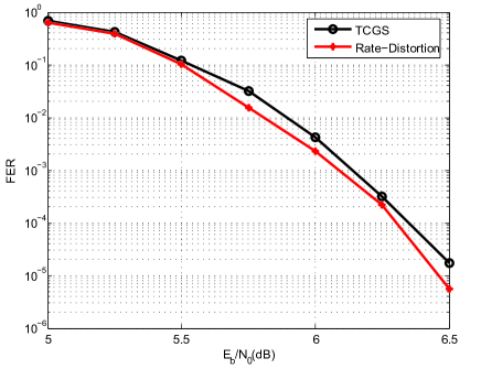
To compare with the rate-distortion approach used in [16], in Fig. 8, we also consider 256ASD-3(RDE,11) algorithm of [16], in which the ASD decoding is performed times, and for each time the computational complexity of the ASD algorithm is roughly [38]. When , the TCGS algorithm has the same maximum number of decoding trials as 256ASD-3(RDE,11) algorithm. Although the former has a little worse performance than the latter, the former requires both less decoding complexity per trial and less average iterations than the latter.
Most existed Chase-type algorithms set a combinatorial number as the maximum testing number. In contrast, the proposed algorithm can take any positive integer as the maximum testing number. Even better, we can set a threshold of the soft weight to terminate the algorithm, that searches the most-likely codeword within an Euclidean sphere rather than a Hamming sphere. The larger the soft discrepancy threshold, the smaller the performance loss. This TCGS algorithm presents a method to simulate the ML lower bound, which is very similar to the one introduced in [17]. If the transmitted codeword is less likely than the estimated codeword from the TCGS decoder, then the ML decoder will surely make an error in this instance as well. We count such instances to generate the lower bound. The ML lower bounds are shown in both Fig. 2 and Fig. 4. In Fig. 2, we see that, for , the performance of TCGS with is very close to the ML lower bound. While for , the performance of TCGS with is about 0.7 dB away from the ML lower bound in Fig. 4. In the simulation, we observe that, frequently, the maximum likelihood candidate occurs much earlier than it is identified. This suggests us to improve the sufficient condition further, as stimulates our future work.
V Conclusions
In this paper, we have presented a new Chase-type soft-decision decoding algorithm for RS codes. The key to develop such an algorithm is the arrangement of all possible flipping patterns in an ordered rooted tree according to the associated lower bounds on their soft weights. With this tree, all flipping patterns can be sorted in a serial manner, which reduces the complexity efficiently when combining with the presented sufficient conditions for optimality. Simulation results show that the proposed tree-based Chase-type algorithm performs well even with less trials on average.
Acknowledgment
The authors are grateful to Mr. Yuan Zhu and Dr. Li Chen for useful discussions.
Appendix A The Minimality of the Minimal Decomposition
There are exactly hypothesized error patterns, which collectively form a coset of the code, . For every , when taking as an input vector, the conventional HDD either reports a decoding failure or outputs a unique codeword c. In the latter case, we say that the flipping pattern f generates the hypothesized error pattern . It can be verified that there exist flipping patterns that can generate the same hypothesized error pattern. In fact, for each , define , which consists of all flipping patterns that generate e.
Proposition 5
Let e be a hypothesized error pattern and f be its associated minimal flipping pattern. Then , and .
Proof:
Since e is a hypothesized error pattern, is a codeword, which can definitely be found whenever the HDD takes as input a vector with . That is, e can be generated by taking (with ) as the input to the HDD. Let be a flipping pattern such that . It suffices to prove that, for and , we have , i. e., , and ). This can be proved by contradiction.
Suppose that . Let be a nonzero component of f. Then e can also be generated by , whose soft weight is less than that of f, a contradiction to the definition of f.
Suppose that . Let and be the nonzero component of f. Then e can also be generated by , whose soft weight is less than that of f, a contradiction to the definition of f.
Obviously, since their support sets have no common coordinates. Suppose that . Let be the atom with rank and be the atom with rank . Then e can also be generated by , whose soft weight is less than that of f, a contradiction to the definition of f. ∎
References
- [1] D. J. Costello Jr., J. Hagenauer, H. Imai, and S. B. Wicker, “Applications of error-control coding,” IEEE Trans. Inform. Theory, vol. 44, no. 6, pp. 2531–2560, 1998.
- [2] A. Al-Dweik, S. L. Goff, and B. Sharif, “A hybrid decoder for block turbo codes,” IEEE Transactions on Communications, vol. 57, no. 5, pp. 1229–1232, May 2009.
- [3] A. J. Al-Dweik and B. S. Sharif, “Non-sequential decoding algorithm for hard iterative turbo product codes - [transactions letters],” IEEE Transactions on Communications, vol. 57, no. 6, pp. 1545–1549, Jun. 2009.
- [4] ——, “Closed-chains error correction technique for turbo product codes,” IEEE Transactions on Communications, vol. 59, no. 3, pp. 632–638, May 2011.
- [5] E. R. Berlekamp, “Nonbinary BCH decoding,” IEEE Trans. Inform. Theory, vol. IT-14, p. 242, 1968.
- [6] L. Welch and E. R. Berlekamp, “Error correction for algebraic block codes,” in Proc. IEEE Int. Symp. Inform. Theory, St. Jovites, Canada, 1983.
- [7] M. Sugiyama, M. Kasahara, S. Hirawawa, and T. Namekawa, “A method for solving key equation for decoding Goppa codes,” Inform. Contr., vol. 27, pp. 87–99, 1975.
- [8] M. Sudan, “Decoding of Reed Solomon codes beyond the error-correction bound,” Journal of Complexity, vol. 13, no. 1, pp. 180–193, 1997.
- [9] V. Guruswami and M. Sudan, “Improved decoding of Reed-Solomon and algebraic-geometric codes,” IEEE Trans. Inform. Theory, vol. 45, no. 6, pp. 1757–1767, Sep. 1999.
- [10] R. Koetter and A. Vardy, “Algebraic soft-decision decoding of Reed Solomon codes,” IEEE Trans. Inform. Theory, vol. 49, pp. 2809–2825, 2003.
- [11] S. Tang, L. Chen, and X. Ma, “Progressive list-enlarged algebraic soft decoding of Reed-Solomon codes,” IEEE Communications Letters, vol. 16, no. 6, pp. 901–904, 2012.
- [12] L. Chen, S. Tang, and X. Ma, “Progressive algebraic soft-decision decoding of Reed-Solomon codes,” IEEE Trans. Commun., vol. 61, no. 2, pp. 433–442, 2013.
- [13] G. D. Forney Jr., “Generalized minimum distance decoding,” IEEE Trans. Inform. Theory, vol. IT-12, no. 2, pp. 125–131, Apr. 1966.
- [14] R. Kotter, “Fast generalized minimum-distance decoding of algebraic-geometry and Reed-Solomon codes,” IEEE Trans. Inform. Theory, vol. 42, pp. 721–737, May 1996.
- [15] S.-W. Lee and B. V. Kumar, “Soft-decision decoding of reed-solomon codes using successive error-and-erasure decoding,” in Proc. IEEE Global Telecommun. Conf., New orleans, LA, Nov. 2008, DOI: 10.1109/GLOCOM.2008.ECP.588.
- [16] P. S. Nguyen, H. D. Pfister, and K. R. Narayanan, “On multiple decoding attempts for Reed-Solomon codes: A rate-distortion approach,” IEEE Trans. Inform. Theory, vol. 57, no. 2, pp. 668–691, Feb. 2011.
- [17] D. Chase, “A class of algorithms for decoding block codes with channel measurement information,” IEEE Trans. Inform. Theory, vol. IT-18, pp. 170–182, Jan. 1972.
- [18] Y. Wu and D. A. Pados, “An adaptive two-stage algorithm for ML and sub-ML decoding of binary linear block codes,” IEEE Trans. Inform. Theory, vol. 49, no. 1, pp. 261–269, Jan. 2003.
- [19] J. Bellorado and A. Kavc̆ić, “Low-complexity soft-decoding algorithms for Reed-Solomon codes—Part I: An algebraic soft-in hard-out Chase decoder,” IEEE Trans. Inform. Theory, vol. 56, no. 3, pp. 945–959, Mar. 2010.
- [20] H. Tang, Y. Liu, M. Fossorier, and S. Lin, “On combining Chase-2 and GMD decoding algorithms for nonbinary block codes,” IEEE Communications Letters, vol. CL-5, pp. 209–211, 2001.
- [21] H. Xia, H. Wang, and J. R. Cruz, “A Chase-GMD algorithm for soft-decision decoding of Reed-Solomon codes on perpendicular recooding channels,” in ICC 2008, vol. 5, 2008, pp. 1977–1981.
- [22] J. Valls, V. Torres, M. J. Canet, and F. M. Garcia-Herrero, “A test vector generation method based on symbol error probabilities for low-complexity chase soft-decision Reed-Solomon decoding,” IEEE Transactions on Circuits and Systems I, vol. 66, no. 6, pp. 2198–2207, Jun. 2019.
- [23] J. Jeong, D. Shin, W. Shin, and J.Park, “An even/odd error detection based low-complexity chase decoding for low-latency rs decoder design,” IEEE Communications Letters, vol. 25, no. 5, pp. 1505–1509, May 2021.
- [24] T. Koumoto, T. Kasami, and L. Shu, “A sufficient condition for ruling out some useless test error patterns in iterative decoding algorithms,” IEICE Trans on Fundamentals, vol. 81, no. 2, pp. 321–326, Feb. 1998.
- [25] D. J. Taipale and M. B. Pursley, “An improvement to generalized-minimum-distance decoding,” IEEE Trans. Inform. Theory, vol. 37, no. 1, pp. 167–172, Jan. 1991.
- [26] T. Kaneko, T. Nishijima, H. Inazumi, and S. Hirasawa, “An efficient maximum-likelihood-decoding algorithm for linear block codes with algebraic decoder,” IEEE Trans. Inform. Theory, vol. 40, no. 2, pp. 320–327, Mar. 1994.
- [27] M. P. Fossorier and S. Lin, “Soft-decision decoding of linear block codes based on ordered statistics,” IEEE Trans. Inform. Theory, vol. 41, no. 5, pp. 1379–1396, 1995.
- [28] J. Jiang and K. R. Narayanan, “Iterative soft-input soft-output decoding of Reed-Solomon codes by adapting the parity-check matrix,” IEEE Trans. Inform. Theory, vol. 52, no. 8, pp. 3746–3756, 2006.
- [29] J. Bellorado, A. Kavc̆ić, M. Marrow, and L. Ping, “Low-complexity soft-decoding algorithms for Reed-Solomon codes—Part II: Soft-input soft-output iterative decoding,” IEEE Trans. Inform. Theory, vol. 56, no. 3, pp. 960–967, Mar. 2010.
- [30] X. Zhang and Y. Zheng, “Generalized backward interpolation for algebraic soft-decision decoding of Reed-Solomon codes,” IEEE Trans. Commun., vol. 61, no. 1, pp. 13–23, Jan. 2013.
- [31] J. Xing, L. Chen, and M. Bossert, “Low-complexity chase decoding of Reed-Solomon codes using module,” IEEE Trans. Commun., vol. 68, no. 10, pp. 6012–6022, Oct. 2020.
- [32] D. Taipale and M. Seo, “An efficient soft-decision Reed-Solomon decoding algorithm,” IEEE Trans. Inf. Theory, vol. IT-40, no. 4, pp. 1130–1139, 1994.
- [33] V. Guruswami and A. Vardy, “Maximum-likelihood decoding of Reed-Solomon codes is NP-hard,” IEEE Trans. Inform. Theory, vol. 51, no. 7, pp. 2249–2256, 2005.
- [34] R. G. Gallager, “Low Density Parity Check Codes,” Cambrideg, MA: MIT Press, 1963.
- [35] H. T. Moorthy, S. Lin, and T. Kasami, “Soft-decision decoding of binary linear block codes based on an iterative search algorithm,” IEEE Trans. Inform. Theory, vol. 43, no. 3, pp. 1030–1040, 1997.
- [36] X. Ma and S. Tang, “Correction to ‘an efficient maximum-likelihood-decoding algorithm for linear block codes with algebraic decoder’,” IEEE Trans. Inform. Theory, vol. 58, no. 6, p. 4073, 2012.
- [37] J. Zhu, X. Zhang, and Z. Wang, “Backward interpolation architecture for algebraic soft-decision Reed-Solomon decoding,” Very Large Scale Integration (VLSI) Systems, IEEE Transactions on, vol. 17, no. 11, pp. 1602–1615, 2009.
- [38] R. J. McEliece, “The Guruswmi-Sudan decoding algorithm for Reed-Solomon codes,” IPN Progress Rep., Tech. Rep. 42-153, 2003.