Observing Dirac’s classical phase space analog to the quantum state

Abstract

In 1945, Dirac attempted to develop a “formal probability” distribution to describe quantum operators in terms of two non-commuting variables, such as position $x$ and momentum $p$ [Rev. Mod. Phys. 17, 195 (1945)]. The resulting quasi-probability distribution is a complete representation of the quantum state and can be observed directly in experiments. We measure Dirac’s distribution for the quantum state of the transverse degree of freedom of a photon by weakly measuring transverse $x$ so as to not randomize the subsequent $p$ measurement. Further, we show that the distribution has the classical-like feature that it transforms (e.g., propagates) according to Bayes’ law.

While formulating quantum theory early in the century, many physicists sought a classical interpretation of the object at its center, the quantum state. The most well-known of these is the Wigner function $W(x,p)$, an attempt to produce a joint probability distribution for a particle’s instantaneous momentum and position (Wigner, 1932). These ‘phase-space’ distributions necessarily violate many of the properties that classical probability distributions must obey. However, they are useful for visualizing concurrent momentum and position features in quantum states, which might be obscurely encoded in the phase of the wavefunction or the off-diagonal elements of the density matrix. Additionally, a non-classical hallmark in the distribution (e.g. negative probabilities) can be used to identify intrinsically quantum states (Hudson, 1974). It is remarkable that even though the quantum state has been an overwhelmingly successful concept and tool for almost a century, our understanding of its nature is still being refined (Harrigan and Spekkens, 2010; *Colbeck2011; *Pusey2012; *Colbeck2012; *Lewis2012). These distributions have contributed to this refinement (Banaszek and Wódkiewicz, 1999; *Brida2002; *Ferrie2008; *Spekkens2008; *Son2009; *Wallman2012) and have helped demarcate the boundary between classical and quantum phenomena (Mari and Eisert, 2012; *Veitch2012).

In quantum physics, Heisenberg’s uncertainty relation implies that a precise joint measurement of position $X$ and momentum $P$ is impossible. Contrast this with classical physics, in which a particle has a definite and unique position $x$ and momentum $p$ at any moment in time, thereby defining its ‘state’. Measuring a classical particle’s state then just entails a joint measurement of $X$ and $P$. Equivalently, one can measure whether a particle is at a particular point $(x,p)$ in ‘phase-space’ (i.e. $X-P$ space) and then raster over $\mathit{x}$ and $\mathit{p}$. And, if the particle is produced in a random process such that it is in a random distribution of states, then repeated measurements at each point will let us find the average result: the probability for the particle to be at that point, $\mathbb{P}(x,p)$, a phase-space probability distribution.

Consider what the quantum version of this measurement would be by beginning with the classical description of this phase-space point, a two-dimensional Dirac delta function centered at $x$ and $p$, $\delta^{\left(2\right)}\left(X-x,P-p\right)$. Crucially, there is no unique nor general method for translating a classical observable to its quantum equivalent (Groenewold, 1946). For example, since they do not commute one must choose an ordering $O$ of quantum operators $\mathbf{X}$ and $\mathbf{P}$ with which to replace classical variables $X$ and $P$:

$$\mathbf{\boldsymbol{\Delta}_{\mathrm{\mathit{O}}}}(x,p)=\left\{\delta^{\left(2\right)}\left(\mathbf{X}-x,\mathbf{P}-p\right)\right\}_{O}.$$ (1)

In this Letter, we experimentally demonstrate the measurement of this operator for the anti-standard ordering (i.e.$\mathbf{P}$ is always to the left of $\mathbf{X}$), $\mathbf{\boldsymbol{\Delta}_{\mathrm{\mathit{AS}}}}(x,p)=\delta(\mathbf{P}-p)\delta(\mathbf{X}-x)=\boldsymbol{\pi}_{p}\boldsymbol{\pi}_{x}$, where $\boldsymbol{\pi}_{m}=\left|m\right\rangle\left\langle m\right|$ is a projector. Numerous other orderings are possible and each corresponds to a distinct point operator $\boldsymbol{\Delta}_{\mathrm{\mathit{O}}}$, which may or may not describe a physical measurement (an ‘observable’). The average result of such a measurement then would be the quantum version of our classical state measurement procedure outlined above.

As usual, this average result is equal to the expectation value of the operator,

$$\left\langle\boldsymbol{\Delta}_{O}(x,p)\right\rangle=\mathrm{Tr}\left[\boldsymbol{\Delta}_{O}(x,p)\boldsymbol{\rho}\right],$$ (2)

where $\boldsymbol{\rho}$ is the density operator describing the quantum state of the particle. It may come as a surprise that this simple, classically motivated measurement procedure will completely determine the quantum state. Whereas classically it gives the probability $\mathbb{P}(x,p)$, the quantum version gives a ‘quasi-probability’ $\mathrm{\mathbb{\widetilde{P}}_{\mathit{\bar{O}}}(x,p)=\left\langle\boldsymbol{\Delta}_{\mathit{O}}\right\rangle}$ (Agarwal and Wolf, 1970a, b), where $\bar{O}$ is the reverse ordering to $O$. That is, for typical orderings $O$, the average result is a phase-space quasi-probability distribution in $x$ and $p$ equivalent to the state of the particle. From this perspective, the Wigner function corresponds to a direct measurement of an $(x,p)$ point observable that has been symmetrically ordered (i.e. the ‘Weyl’ ordering $\mathrm{W}$, with $W=\bar{W}$): $\mathrm{\mathbf{\boldsymbol{\Delta}_{\mathit{W}}=R}}_{\pi}(x,p)/\pi$ (Royer, 1977), where $\mathbf{R}_{\pi}$ is the parity of a particle about point $(x,p)$. The normal $N$ ordering ($\mathbf{a^{\dagger}}$ to the left of $\mathbf{a}$, where $\mathbf{a}$ is the usual lowering operator $\mathbf{a}=\mathbf{X}+i\mathbf{P}$ ) and its reverse, anti-normal $AN$, correspond to the other two well-known quasi-probability distributions, the Husimi Q function (Husimi, 1940) ($\mathbb{\widetilde{P}}{}_{\mathit{N}}$,$\mathbf{\boldsymbol{\Delta}_{\mathrm{\mathit{AN}}}}(\alpha=x+ip)=\left|\alpha\right\rangle\left\langle\alpha\right|/\pi$, i.e. a projection onto a coherent state $\left|\alpha\right\rangle$ (Agarwal and Wolf, 1970a) ) and the Glauber-Sudarshan P distribution (Glauber, 1963; *Sudarshan1963) ($\mathbb{\widetilde{P}}_{\mathit{AN}}$, $\mathbf{\boldsymbol{\Delta}_{\mathrm{\mathit{N}}}}$ is unphysical ). The Wigner and Q functions have been directly measured in various physical systems (Vogel and Risken, 1989; *Banaszek1996; *Leonhardt1997; *Lutterbach1997; *Bertet2002; *Kanem2005; *Hofheinz2009; *Laiho2010), including the transverse state of a photon (Mukamel et al., 2003; *Smith2005).

Figure 1: Experimental setup to directly measure the Dirac quasi-probability distribution $\mathrm{\mathbb{\widetilde{P}}}(x,p)$ of the transverse state of a photon. Photons emerge from a single mode fiber and are collimated to produce an identical ensemble in an initial pure state. This is optionally transformed to a mixed state by noise introduced by an oscillating glass plate. A weak measurement of transverse position $\boldsymbol{\pi}_{x}=\left|x\right\rangle\left\langle x\right|$ is implemented by a small polarization rotation $\varphi=12.92^{\circ}$ created by a quartz sliver at $x$. This weak measurement is read out jointly with the transverse momentum $p$ by using a camera, polarizer and quarter waveplate in the Fourier transform plane to measure $\left\langle\boldsymbol{\pi}_{p}\boldsymbol{\sigma}^{-}\right\rangle=\sin\varphi\mathrm{\mathbb{\widetilde{P}}}(x,p)$. We repeat this measurement after displacing the camera from the Fourier transform plane by $\Delta z$ in order to investigate how the distribution propagates in space.

In 1945, Dirac wrote “On the analogy between classical and quantum mechanics,” (Dirac, 1945) in which he introduced what we call the ‘Dirac distribution’ as a classical-like representation of a quantum operator, such as the density operator $\boldsymbol{\rho}$. Over the past 90 years this distribution has been repeatedly rediscovered (McCoy, 1932; Kirkwood, 1933; *Terletsky1937; *Rivier1951; *Barut1957; *Margenau1961; *Levin1964; *Rihaczek1968; *Ackroyd1970). It has since been realized that the Dirac distribution is $\mathrm{\mathbb{\widetilde{P}}}_{\mathit{S}}(x,p)$, the standard ordered quasi-probability distribution and its complex conjugate is $\mathbb{\widetilde{P}}_{A\mathit{S}}(x,p)$ (Agarwal and Wolf, 1970a; Praxmeyer and Wódkiewicz, 2003; Chaturvedi et al., 2006). Despite being the product of one of the founders of quantum theory, there has been little experimental investigation of the Dirac distribution over the past 90 years. The impediment has been that although its direct measurement appears simple, i.e. a measurement of position then momentum, one quickly notices that $\mathbf{\boldsymbol{\Delta}_{\mathrm{\mathit{AS}}}}=\boldsymbol{\pi}_{p}\boldsymbol{\pi}_{x}$ is non-Hermitian and thus should not be an observable. Physically, this is enforced by the fact that a measurement of $\boldsymbol{\pi}_{x}=\delta(\mathbf{X}-x)$ will disturb and hence invalidate the subsequent measurement of $\boldsymbol{\pi}_{p}=\delta(\mathbf{P}-p)$, making a joint measurement impossible.

Two ways in which measurement-induced disturbance can be minimized in quantum physics are: 1. by lowering the precision, $\delta(x)\rightarrow$$\Delta x$, and 2. by decreasing the certainty of the measurement,$\mathrm{Prob}(x_{system}|x_{measured})\ll 1$. An example of the second approach is weak measurement: by reducing the coupling between the system and the measurement apparatus, the result from any one trial becomes uncertain (Pryde et al., 2005; *Resch2004; *Mir2007; *Williams2008; *Hosten2008; *Lundeen2009; *Yokota2009; *Dixon2009; *Feizpour2011; *Kocsis2011). Reducing the coupling similarly reduces the disturbance (i.e. back-action). Moreover, by averaging over many trials an average result can still be found to arbitrarily low uncertainty. Remarkably, the Dirac distribution can be measured simply by replacing the first measurement by a weak measurement (Aharonov et al., 1988) of $\boldsymbol{\pi}_{x}$, as we showed in Ref. (Lundeen and Bamber, 2012) (see also the related work (Arthurs and Kelly, 1965; *Johansen2008; *Kalev2012; *DiLorenzo2013; *Wu2013)).We termed the average joint result of this weak-strong position-momentum measurement, the ‘weak average’. In the zero-coupling limit, it is (Lundeen and Bamber, 2012),

$$\left\langle\boldsymbol{\pi}_{p}^{\mathrm{s}}\boldsymbol{\pi}_{x}^{\mathrm{w}}\right\rangle_{\rho}=\mathrm{Tr}\left[\boldsymbol{\pi}_{p}\boldsymbol{\pi}_{x}\boldsymbol{\rho}\right]=\left\langle\mathbf{\boldsymbol{\Delta}_{\mathrm{\mathit{AS}}}}(x,p)\right\rangle=\mathrm{\mathbb{\widetilde{P}}}_{\mathit{S}}(x,p),$$ (3)

where $\mathrm{\mathbb{\widetilde{P}}}_{\mathit{S}}$ is the Dirac distribution (see Supp. Mat.). The superscripts s and w denote strong (i.e. normal) and weak measurements, respectively. (From here on, we omit the $S$ subscript as we will deal exclusively with the Dirac distribution.) As an expectation value of a non-Hermitian operator, the weak average is complex in general (Jozsa, 2007). The real component manifests itself in the usual pointing variable of the measurement apparatus while the imaginary component manifests itself in the conjugate variable, as we will describe later using our specific experiment as an example. It follows that, unlike the Wigner function and other aforementioned quasi-probabilities, the Dirac distribution is complex.

The Dirac distribution $\mathrm{\mathbb{\widetilde{P}}}(x,p)$ possesses the key feature that it can be manipulated according Bayes’ Theorem despite the fact that it is not a true probability (Steinberg, 1995; Hofmann, 2012). For example, we could calculate the conditional quasi-probability of $x$ given $p$: $\mathrm{\mathbb{\widetilde{P}}}(x|p)=\mathrm{\mathbb{\widetilde{P}}}(x,p)/\mathrm{\mathbb{\widetilde{P}}}(p)$, where $\mathrm{\mathbb{\widetilde{P}}}(p)\equiv\left\langle\boldsymbol{\pi}_{p}^{\mathrm{w}}\right\rangle_{\rho}=\mathbb{P}(p)$ is defined in analogy to the weak average. One could also directly measure $\mathrm{\mathbb{\widetilde{P}}}(x|p)$ by following our naive procedure above but only keeping the results for $X$ in those cases where $P=p$. For $p=0$, this is a succinct description of our previously introduced procedure to directly measure the quantum wavefunction $\Psi(x)$ (Lundeen et al., 2011). In this light, one would write $\Psi(x)\propto\mathrm{\mathbb{\widetilde{P}}}(x|p=0)$, which provides wavefunction with a pithy description: It is the quasi-probability of $x$ given that $p$ was found to be zero.

Figure 2: Directly measured Dirac distributions for a (a) pure and a (b) mixed state. In both (a) and (b), the left and right insets are the directly measured real and imaginary parts of the Dirac distribution $\mathrm{\mathbb{\widetilde{P}}}(x,p)$. From these we calculate the magnitude (upper plot) and phase (lower plot) of the distribution. In the axes, transverse $x$ corresponds to the position of the quartz sliver and, thus, the weak measurement of $\left|x\right\rangle\left\langle x\right|$; transverse $k=p/\hbar$ is the transverse wavevector, which is proportional to the transverse position in the Fourier transform plane at the camera sensor (see text).

Unlike our wavefunction measurement procedure (Lundeen et al., 2011), the measurement of the Dirac distribution can also determine the state of a system that is ‘mixed’. In this case, the state is fully characterized by a density operator $\boldsymbol{\rho}$ rather than a wavefunction $\Psi(x)$. The density operator is a generalization of the wavefunction (i.e. a ‘pure’ state) that can incorporate classical noise and the effects of entanglement with other systems. It is widely used in statistical mechanics, quantum chemistry, quantum information and atomic physics.

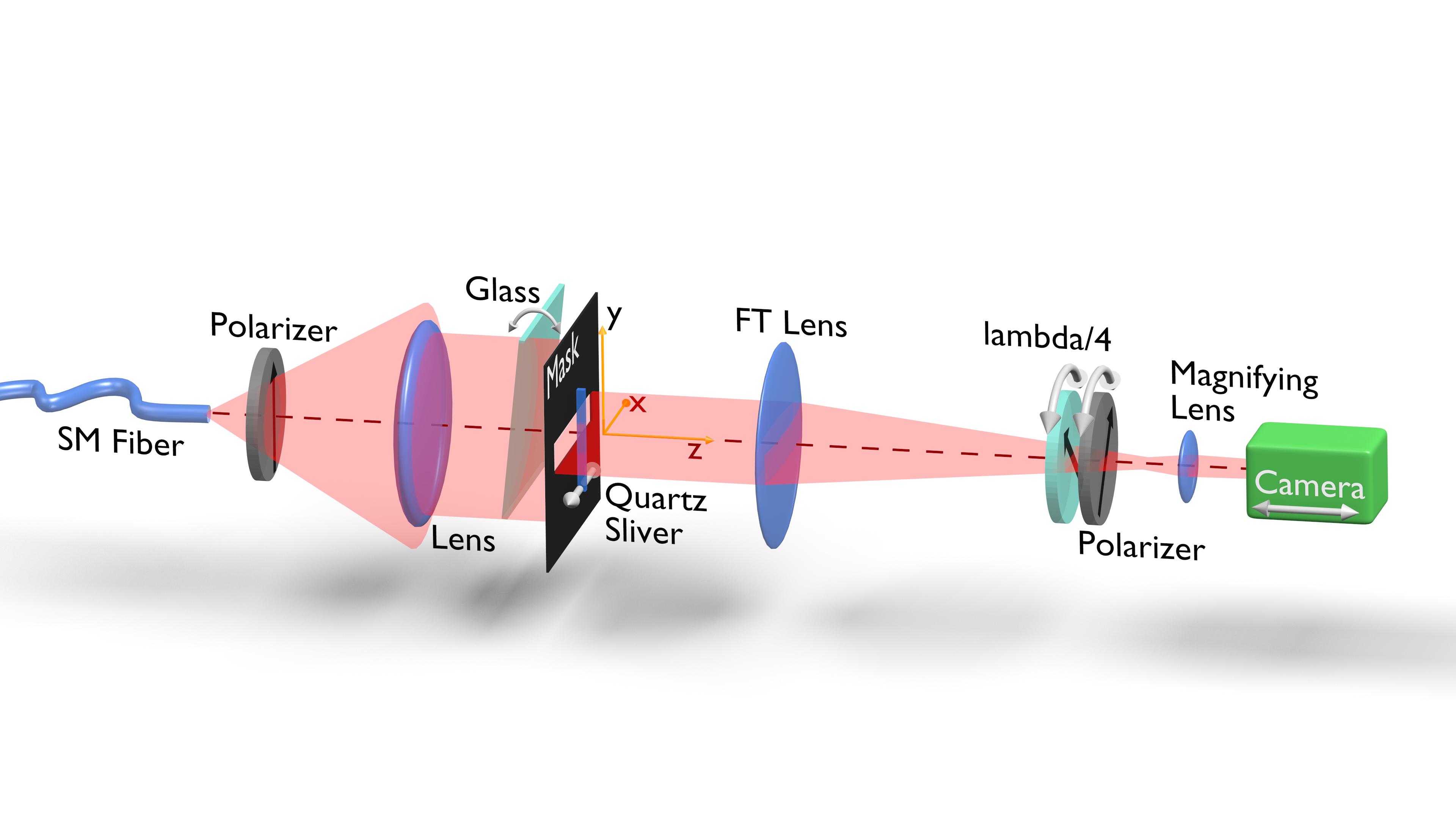
As an example, we measure the Dirac distribution of the quantum state corresponding to the transverse position of a photon for mixed and pure states. We clarify what we mean by the photon’s quantum state in the Supplementary Material. Recent work has measured the Dirac distribution in a discrete system (Salvail et al., 2013) but only for the pure case, and only in a simple two-level system. Shown in Fig. 1, our experimental setup builds on the one in Ref. (Lundeen et al., 2011). Our photons are produced by an attenuated laser (wavelength=780 nm) and coupled into a single-mode fiber. Although we do not use single-photon states, one can say that every photon that exits the fiber output will have the same transverse state; they form an identical ensemble of particles. The photons are linearly polarized and collimated by a convex lens (achromat, focal length $f=30$ cm, diameter $d=5$ cm) and sent through an aperture (x$\times$y dimensions=44 mm$\times$2 mm). Unlike in Ref. (Lundeen et al., 2011), just before the lens, we introduce phase-noise by rotating a 4 mm thick glass plate by 4 degrees about a horizontal rotation axis at 11 Hz, thereby generating many waves of phase delay. The plate extends only over one half of the transverse state. With the glass stationary, the transverse state’s phase is discontinuous at the position of the plate edge. With it oscillating, the two halves of the state are completely incoherent over the time-scale of our measurements and, thus, the state is mixed.

We divide the weak measurement of $\boldsymbol{\pi}_{x}=\left|x\right\rangle\left\langle x\right|$ into two stages: coupling and readout. The coupling stage occurs just after the collimating lens. This is the plane in space at which we measure the Dirac distribution of the photon ensemble. Here, a quartz sliver (width $\Delta x=1$ mm) rotates the photon polarization (initially $0^{\circ}$) to $\varphi$ degrees at position $x$. For $\varphi=90^{\circ}$ this would be a strong measurement, whereas by setting $\varphi\ll 90^{\circ}$ our measurement becomes weak. The sliver is also slightly tilted about the x-axis in order to null any phase shift it induces. As described in Ref. (Lundeen et al., 2011), we can readout by measuring $\left\langle\boldsymbol{\pi}_{x}^{\mathrm{w}}\right\rangle=(\left\langle s\right|\boldsymbol{\sigma}_{x}\left|s\right\rangle-i\left\langle s\right||\boldsymbol{\sigma}_{y}\left|s\right\rangle)/\sin\varphi=\left\langle s\right|\boldsymbol{\sigma^{-}}\left|s\right\rangle/\sin\varphi$, where $\left|s\right\rangle$ is the polarization state of the photon, $\boldsymbol{\sigma}_{x}$ and $\boldsymbol{\sigma}_{y}$ are the Pauli operators, and $\boldsymbol{\sigma}^{-}=\boldsymbol{\sigma}_{x}+i\boldsymbol{\sigma^{-}}$ is the lowering operator (Lundeen and Resch, 2005). The real part and imaginary parts of the weak value are proportional to the shift from zero of the average value of $\boldsymbol{\sigma}_{x}$ and $\boldsymbol{\sigma}_{y}$, respectively. Thus, as expected the two parts separately appear in conjugate variables of our measurement apparatus, that is, in the linear and circular polarizations.

Figure 3: Density matrices $\rho$ for a (left plots) pure and a (right plots) mixed state, calculated from data presented in Fig. 2. The upper plots and lower plots correspond to the real and imaginary parts of $\rho$, respectively.We have divided the diagonals by $\cos(\varphi)$ to correct for effect of the measurement back-action (see the Supp. Mat. for details)

In order to perform a joint measurement of $\boldsymbol{\pi}_{p}\boldsymbol{\pi}_{x}$ we must make polarization measurements at each momentum. To do so, a lens (achromat, $f_{FT}=$1 m, $d=$5 cm) is placed one focal length after the sliver. The Fourier transform (FT) of the quantum state forms in the plane one focal length past the lens. Consequently, the transverse position $x_{FT}$ in this FT plane is proportional to the transverse momentum $p$ of the photon at the sliver. We magnify ($M=4.935$) by another lens ($f=35$ mm, $d=2.5$ cm) so that the final scaling is $p=x_{FT}h/(f_{FT}M\lambda)$, where $h$ is Planck’s constant. To readout $\left\langle\boldsymbol{\pi}_{x}^{\mathrm{w}}\right\rangle$ we project onto a circular or linear polarization by inserting a quarter-waveplate ($\mathrm{lambda}/4$) and/or polarizer (Pol, Nanoparticle Linear Film Polarizer, Thorlabs LPVIS50) just before the magnifying lens. Then, position and momentum are jointly measured by measuring $\boldsymbol{\pi}_{p}\boldsymbol{\sigma}^{-}$. We do so by recording the average number of photons $N_{p,j}$ arriving at each transverse position $x_{FT}$ on a camera sensor (Basler acA1300-30um, pixel size: 3.75$\mathrm{\mu m}$$\times$3.75$\mathrm{\mu m}$, x$\times$y array size: 1296$\times$966, 12 bit) for two pairs of polarization measurements: $j=45^{\circ}$ and $-45^{\circ}$ polarizations, and right ($\circlearrowleft$) and left-hand ($\circlearrowright$) circular polarizations. For $\varphi\ll 90^{\circ},$ the differences in each pair are proportional to the real and imaginary parts of the Dirac distribution,

$$\left\langle\boldsymbol{\pi}_{p}\boldsymbol{\sigma}^{-}\right\rangle=\frac{N_{p,45^{\circ}}-N_{p,-45^{\circ}}}{N_{p,45^{\circ}}+N_{p,-45^{\circ}}}-i\frac{N_{p,\circlearrowleft}-N_{p,\circlearrowright}}{N_{p,\circlearrowleft}+N_{p,\circlearrowright}}=\mathrm{\mathbb{\widetilde{P}}}(x,p)\sin\varphi,$$ (4)

where the expectation value is now an average over the polarization and transverse momentum state of the photon ensemble. Each polarization measurement is a 1.8 s camera exposure in which we average along the $y$ dimension to arrive at a vector $N_{p,j}$. We take the mean of the weak average over ten scans of $x$.

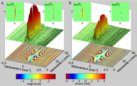
We directly measure the Dirac distribution $\mathrm{\mathbb{\widetilde{P}}}(x,p)$ for the transverse quantum state by measuring these polarization differences for every $p$ as a function of the sliver position $x$, which we move in steps of 1 mm across aperture of the collimating lens. The insets of Fig. 2 plot this pair of polarization differences as the real and imaginary parts of $\mathrm{\mathbb{\widetilde{P}}}(x,p)$ according to Eq. 4. Fig. 2 (a) and (b) display the measured Dirac distribution for the case where the glass plate is stationary (pure state) and oscillating (mixed state), respectively. As can be seen in the lower plots, there is a state-independent phase of $\exp(-ixk),$ inherent to the Dirac distribution, imposed on the underlying 2-d form of the state in (a) and (b). This overlay phase structure allows one to immediately see phase jumps, such as the one in the pure state (a) at $x=$25 mm (the glass edge) due to increased optical path length through the glass. In contrast, in the mixed state (b), the phase fringes on either side of $x=$25 mm are unrelated, a signature of the lack of phase coherence across this point. Looking now at the magnitude, shown in the upper plots, both the mixed and pure states exhibit a depression at $x=25$ mm, likely due to photons being scattered out of the apparatus by the glass edge. In the momentum direction, the width of the mixed state is broader than the pure state, as is expected due to the reduced spatial coherence of the former. This is accompanied by a decreased magnitude since the distribution is normalized to one. These distinctive features suggest that the Dirac distribution provides a useful way to visualize key characteristics of pure and mixed quantum states.

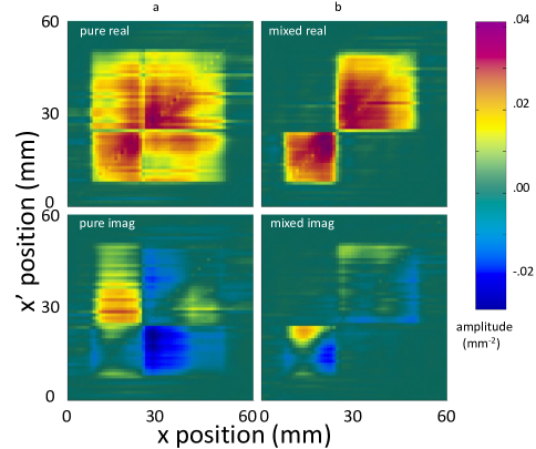
The Dirac distribution is related in a simple way to the position density matrix of the state, $\rho(x,x^{\prime})=\left\langle x\right|\boldsymbol{\rho}\left|x^{\prime}\right\rangle=\mathrm{FT}\left[\mathrm{\mathbb{\widetilde{P}}}(x,p)\exp(ipx/h)\right](x^{\prime})$, where the Fourier transform FT is performed with respect to momentum $p$ (Chaturvedi et al., 2006). In Fig. 3, we plot the position density matrix for each of the Dirac distributions from Fig. 2. For the pure state Fig. 3 (a), the hard edges of the aperture form a square outline in $\boldsymbol{\rho}$ and the phase jump now appears at both $x=$25 mm and $x^{\prime}=$25 mm. Strikingly, in the mixed state in Fig. 3 (b) the off-diagonal regions for $x$$\leq 25$ mm, $x^{\prime}$>25 mm, and the reverse are close to zero. This is indicative of the lack of coherence between the part of the state that passes through the oscillating glass and the part that does not. This shows that we can successfully measure the Dirac distribution for a transverse quantum state and that it correctly determines the state of a mixed system. Since we are not in the limit of a zero interaction-strength measurement ($\varphi=0$), there will still be some backaction due to the measurement. While in the Dirac distribution this leads to minor offsets $\mathrm{\mathbb{\widetilde{P}}}(x,p)\rightarrow\mathrm{\mathbb{\widetilde{P}}}(x,p)-\mathrm{Prob}(x)(1-\cos(\varphi))$ everywhere, in the density matrix it leads solely to a suppression, by $\cos(\varphi)$, of the diagonals, which we correct for in Fig 3 (see Supp. Mat.).

Figure 4: Evolution of the quantum state by Bayes’ theorem. (a) A series of directly measured Dirac distributions propagated from the mixed state in Fig. 2 (b) to a plane translated by $\Delta z=$ (i) 8.4 cm, (ii) 16 cm, and (iii) 32.5 cm past the Fourier transform plane (by moving the camera). (b) The theoretical prediction for the propagated distributions found using Bayes’ theorem, as in Eq. 8. In all (a-b) (i-iii), the bottom plot is Dirac distribution’s phase and both the inset and top plot are its magnitude. As in Fig. 2, the transverse $x$ axis is the position of the weak measurement, whereas transverse $k^{\prime}$ now corresponds to the transverse position on the camera (which is no longer proportional to momentum).

The compatibility of Bayes’ theorem with the Dirac quasi-probability distribution goes beyond the simple example we gave earlier. The simplicity of Dirac distribution allows us to generalize its theoretical definition to multiple variables, e.g., $\mathrm{\mathbb{\widetilde{P}}}(x,q^{\prime},k^{\prime},p)=\left\langle\delta(\mathbf{P}-p)\delta(\mathbf{K^{\prime}}-k^{\prime})\delta(\mathbf{Q^{\prime}}-q^{\prime})\delta(\mathbf{X}-x)\right\rangle$=$\mathrm{Tr}\left[\boldsymbol{\pi}_{p}\boldsymbol{\pi}_{k^{\prime}}\boldsymbol{\pi}_{q^{\prime}}\boldsymbol{\pi}_{x}\boldsymbol{\rho}\right]$ , where $Q^{\prime}$ and $K^{\prime}$ are another two continuous variables (e.g. the photon position and momentum at a later time after undergoing some evolution). Hoffman showed that with the above theoretical definition of $\mathrm{\mathbb{\widetilde{P}}}(x,q^{\prime},k^{\prime},p)$ one can propagate the Dirac distribution $\mathrm{\mathbb{\widetilde{P}}}(x,k)$ in time by applying Bayes’ theorem (Hofmann, 2012):

$$\mathrm{\mathbb{\widetilde{P}}}(q^{\prime},k^{\prime}) = \sum_{x,p}\mathrm{\mathbb{\widetilde{P}}}(x,q^{\prime},k^{\prime},p)$$ (5)

$$= \sum_{x,p}\mathrm{\mathbb{\widetilde{P}}}(q^{\prime},k^{\prime}|x,p)\cdot\mathrm{\mathbb{\widetilde{P}}}(x,p),$$ (6)

where $\mathrm{\mathrm{\mathbb{\widetilde{P}}}}(q^{\prime},k^{\prime}|x,p)=\mathrm{\mathbb{\widetilde{P}}}(x,q^{\prime},k^{\prime},p)/\mathrm{\mathbb{\widetilde{P}}}(x,p)=\left\langle p|k^{\prime}\right\rangle\left\langle k^{\prime}|q^{\prime}\right\rangle\left\langle q^{\prime}|x\right\rangle/\left\langle p|x\right\rangle$ is independent of the quantum state. This four dimensional generally complex conditional quasi-probability is a propagator of an arbitrary point in $x,p$ phase-space to any point in $q^{\prime},k^{\prime}$ phase-space. In the context of quantum information, it functions like a superoperator (i.e. it transforms between density operators) and can encompass both unitary and non-unitary evolution of any quantum process (see (Hofmann, 2013; *Morita2013) for further development of this concept). Note that this is very different from using Bayes’ theorem to update a prior quantum state based on the incomplete information about the system provided by classical positive-valued statistics, e.g. POVMs (as was studied in (Barnett et al., 2000; *Caves2002)). In particular, here, as with classical probability distributions, one can directly apply Bayes’ theorem to update the Dirac quasi-probability distribution and evolve it as a function of space or time.

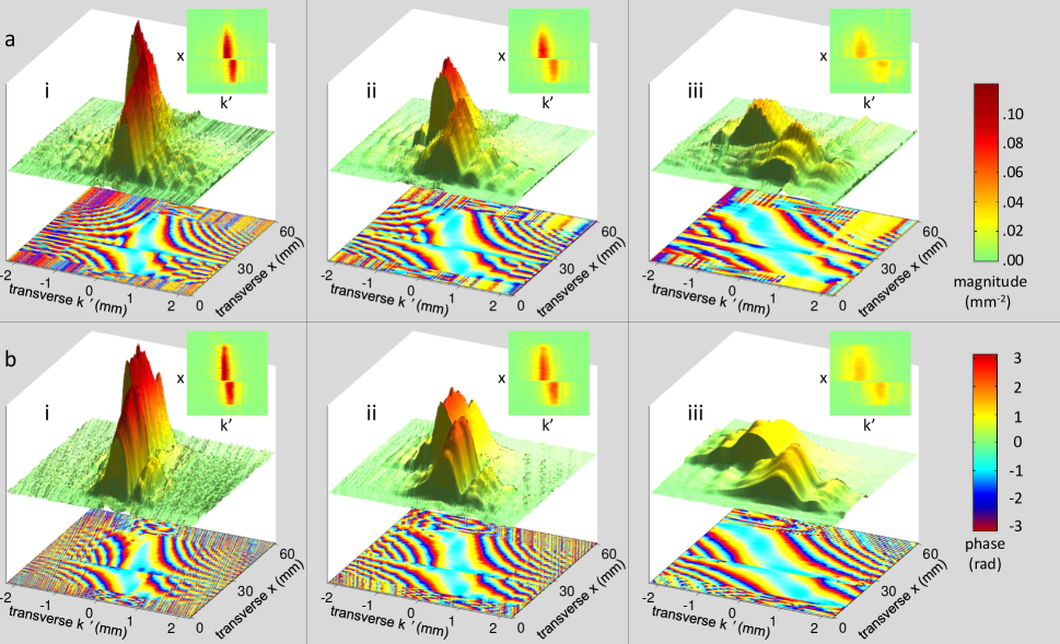
We now describe a demonstration of this Bayesian propagation. For the sake of experimental simplicity, we only update one of the variables in the Dirac distribution $\mathrm{\mathrm{\mathbb{\widetilde{P}}}(x,p)}$ to arrive at $\mathrm{\mathrm{\mathbb{\widetilde{P}}}}(x,k^{\prime})=\left\langle\boldsymbol{\pi}_{k^{\prime}}^{\mathrm{s}}\boldsymbol{\pi}_{x}^{\mathrm{w}}\right\rangle_{\rho}$. By moving the camera back from the re-imaged Fourier transform plane so that the photons travel a further distance $\Delta z$ before being detected, we change our strong measurement of $P$ to one of $K^{\prime}$, which is a combination of $X$ and $P$ (Lohmann, 1993) (See Supp Mat.). Then we make a joint weak-strong measurement of $X$ and $K^{\prime}$ in exactly the same manner as we did for the Dirac distribution to experimentally measure $\mathrm{\mathrm{\mathbb{\widetilde{P}}}}(x,k^{\prime})$. We repeat the experiment [Fig 4. (a)] and theoretical [Fig 4. (b)] Bayes’ propagation (see Supp. Mat.) for three values of $\Delta z,$ and plot the results in Fig. 4 (i-iii). As $\Delta z$ is increased, the distributions in Fig. 4 exhibit a broadening of $\mathrm{\mathrm{\mathbb{\widetilde{P}}}}(x,k^{\prime})$ in the $K^{\prime}$ direction. This is due to the broad width of the photon state in $X$ and the fact that the $X$ portion of the hybrid $X,P$ variable $K^{\prime}$ increases as $\Delta z$ is increased. Also apparent is a growing $k^{\prime}$ displacement of the $x>25$mm portion of the state as $\Delta z$ is increased. This is consistent with a wedge in our oscillating glass plate of 0.4 arcseconds. Evidently, each of the three pairs of experimental and theoretical distributions agree well in a qualitative manner, which confirms the applicability of classical-like Bayesian propagation.

In conclusion, by experimentally measuring the Dirac quasi-probability distribution we have completely determined a mixed quantum state. We have also demonstrated that the Dirac distribution measured at different spatial planes are related by Bayes’ law, which therefore acts as a propagator of the quasi-probability. Quasi-probability distributions like the Q, P, or Wigner function reflect the arbitrary choice of the operator ordering (normal, anti-normal, or symmetric) that embodies the inherent incompatibility of quantum and classical physics. Missing from this list has been the standard ordering, the Dirac quasi-probability distribution, which has three outstanding features: 1. Its measurement is simple and similar to the classical equivalent. 2. It is compatible with Bayes’ theorem, with which we can propagate it to other points in space or time. 3. In the limit of a pure quantum state, it reduces to quantum wavefunction itself.

Appendix A Supplementary Material for ‘Observing Dirac’s classical phase space analog to the quantum state’

A.1 Weak-strong measurement of joint operators

In this section, we show that the joint weak-strong measurement of position-momentum projectors is equal to the average given by the standard Born rule: $\left\langle\boldsymbol{\pi}_{p}^{\mathrm{s}}\boldsymbol{\pi}_{x}^{\mathrm{w}}\right\rangle_{\rho}=\mathrm{Tr}\left[\boldsymbol{\pi}_{p}\boldsymbol{\pi}_{x}\boldsymbol{\rho}\right]$. We call this the ‘weak average’.This result was proven using an explicit Hamiltonian that models the process of this joint measurement in our previous Letter Lundeen and Bamber (2012). That result was shown to be true for general observables and for a final measurement that can be either weak or strong. Here, we give a less rigorous but more intuitive derivation of this result by restricting ourselves to observables that are projectors and to a strong final measurement.

We begin with a review of the ‘weak value’ in this context. One starts with an ensemble of quantum systems all in an identical initial state $\left|\Psi\right\rangle$. For each member of the ensemble, one weakly measures a projector $\boldsymbol{\pi}_{a}$ and then strongly measures another observable $\mathbf{C}$. Consider the sub-ensemble where that second measurement gave outcome $c$. In the limit of zero-interaction strength, the average result of measurement $\mathrm{\mathbf{A}}$ in this sub-ensemble is called the weak value Aharonov et al. (1988):

$$\left\langle\mathrm{\mathbf{\boldsymbol{\pi}_{a}}}\right\rangle_{\Psi c}=\frac{\left\langle c\right|\mathrm{\mathrm{\boldsymbol{\pi}_{a}}}\left|\Psi\right\rangle}{\left\langle c|\Psi\right\rangle}.$$

This is an average result conditioned (i.e. post-selected) on outcome $c$. If we instead want $\left\langle\boldsymbol{\pi}_{c}^{\mathrm{s}}\boldsymbol{\pi}_{a}^{\mathrm{w}}\right\rangle_{\Psi}$, the average result of $\mathrm{\mathbf{\boldsymbol{\pi}_{a}}}$ and $c$, then, as usual, one multiplies the conditional average of $\mathrm{\mathbf{\boldsymbol{\pi}_{a}}}$ by $\mathrm{Prob}(c)=\left\langle c|\Psi\right\rangle\left\langle\Psi|c\right\rangle$:

$$\left\langle\boldsymbol{\pi}_{c}^{\mathrm{s}}\boldsymbol{\pi}_{a}^{\mathrm{w}}\right\rangle_{\Psi} = \frac{\left\langle c\right|\mathrm{\mathrm{\boldsymbol{\pi}_{a}}}\left|\Psi\right\rangle}{\left\langle c|\Psi\right\rangle}\left\langle c|\Psi\right\rangle\left\langle\Psi|c\right\rangle$$ (7)

$$= \left\langle c\right|\mathrm{\mathrm{\boldsymbol{\pi}_{a}}}\left|\Psi\right\rangle\left\langle\Psi|c\right\rangle$$ (8)

Now, we want to generalize this result to mixed states, $\boldsymbol{\rho}=\sum_{j}$$\lambda_{j}$$\left|\Psi_{j}\right\rangle$$\left\langle\Psi_{j}\right|$. Each state in this sum contributes a joint weak-strong average $\left\langle\boldsymbol{\pi}_{c}^{\mathrm{s}}\boldsymbol{\pi}_{a}^{\mathrm{w}}\right\rangle_{\Psi_{j}}$:

$$\left\langle\boldsymbol{\pi}_{c}^{\mathrm{s}}\boldsymbol{\pi}_{a}^{\mathrm{w}}\right\rangle_{\rho} = \sum_{j}\lambda_{j}\left\langle\boldsymbol{\pi}_{c}^{\mathrm{s}}\boldsymbol{\pi}_{a}^{\mathrm{w}}\right\rangle_{\Psi_{j}}$$

$$= \sum_{j}\lambda_{j}\left\langle c\right|\mathrm{\mathrm{\boldsymbol{\pi}_{a}}}\left|\Psi_{j}\right\rangle\left\langle\Psi_{j}|c\right\rangle$$

$$= \left\langle c\right|\mathrm{\mathrm{\boldsymbol{\pi}_{a}}}\sum_{j}\lambda_{j}\left|\Psi_{j}\right\rangle\left\langle\Psi_{j}|c\right\rangle$$

$$= \left\langle c\right|\mathrm{\mathrm{\boldsymbol{\pi}_{a}}}\boldsymbol{\rho}\left|c\right\rangle$$

$$= \mathrm{Tr}\left[\boldsymbol{\pi}_{c}\boldsymbol{\pi}_{a}\boldsymbol{\rho}\right].$$

If $a=x$ and $c=p$, this proves our result.

A.2 The Photon Wavefunction

Over the last twenty years, the concept of a photon’s wavefunction has been clarified. The photon’s full quantum state describes its freqency-time, position-momentum, and polarization degrees of freedom. The quantum state formalism has been successfully used in hundreds, if not thousands, of papers to theoretical describe the physics of single and entangled photons in experiments, so one might ask why there is any controversy. Confusion about this concept largely arose because the concept of the wavefunction was introduced in terms of the non-relativistic Schrï¿œdinger Equation, yet 1. the Schrï¿œdinger Equation contains a mass parameter, whereas the photon is massless, 2. The position operator in Schrï¿œdinger Equation is not a true observable for photons; they are naturally relativistic and cannot be localized to an exact position Newton and Wigner (1949). Compounding this confusion is the fact that Dirac derived the second quantization (i.e. Quantum Electrodynamics) for the electromagnetic field blackbefore he considered its first quantization.

In short, the answer to this confusion is that Maxwell’s equations play the same role to the photon as the Schrï¿œdinger Equation does to, say, an electron Sipe (1995); Bialynicki-Birula (1996); Smith and Raymer (2007). blackThe solution to these equations is the first quantization of the electromagnetic field, the wavefunction of the photon. In fact, Maxwell’s Equations can be combined into a single equation that has the same analytic form as the Schrï¿œdinger Equation. This resolves issue number 1; the Schrï¿œdinger Equation is not valid for a photon, but there is an equation that blackhas the same form as the Schrï¿œdinger Equation that is valid. The resolution to issue number 2 comes in two limits. In the limit of relativistic massive particles on should use the relativistic Schrï¿œdinger Equation, in which the standard position observable is not valid Newton and Wigner (1949). That is, both photons and electrons do not have simple position observable in the relativistic limit. In fact, there is an inherent contradiction in the non-relativistic Schrï¿œdinger Equation: an electron localized to a point will contain infinite momentum components, and, hence, will be relativistic.

Consequently, the position observable in the Schrï¿œdinger Equation is only a valid approximation in certain limits. The same holds for the photon; when one is in both the paraxial limit and in the limit where the slowly varying frequency envelope amplitude approximation is valid Deutsch and Garrison (1991); Aiello and Woerdman (2005), the photon wavefunction can be written as $\Psi(\overset{\rightharpoonup}{p},\sigma)$, where $\overset{\rightharpoonup}{p}=(p_{x},p_{y},p_{z})$ is the photon’s momentum and $\sigma=H,V$ is the polarization of the photon ($H$=horizontal, $V$=vertical). In these limits, $p_{z}=hf/c$ and $z=t/c$, where $f$ is the photon’s frequency and $t$ is photon’s time ($h$ is Heisenberg’s constant and $c$ is the speed of light). These parameters are all defined relative to some time-space coordinate system. In these limits, transverse positions $x$ and $y$; transverse momenta $p_{x}$ and $p_{y}$; frequency $f$ (or $p_{z}$); and time $t$ (or $z$) can each be measured as an observable. Moreover, in these limits, the photon wavefunction is normalized to unity in the same manner as the electron wavefunction:

$$\sum_{\sigma}\int d\overset{\rightharpoonup}{p}\left|\Psi(\overset{\rightharpoonup}{p},\sigma)\right|^{2} = 1$$

$$\sum_{\sigma}\iiint dxdydz\left|\Psi(x,y,z,\sigma)\right|^{2} = 1$$

$$\sum_{\sigma}\iiint dp_{x}dp_{y}df\left|\Psi(p_{x},p_{y},f,\sigma)\right|^{2} = 1.$$

These normalizations show some of the many equivalent ways of expressing the photon wavefunction.

The relation to the second quantization of light is that the wavefunction of the photon becomes a ‘mode’ in which photons can be created such that,

$$\mathbf{a}_{\Psi}^{\dagger}=\sum_{\sigma}\iiint dp_{x}dp_{y}df\Psi(p,f,\sigma)\mathbf{a}_{p_{x},p_{y},f,\sigma}^{\dagger},$$

where $\mathbf{a}_{p_{x},p_{y},f,\sigma}^{\dagger}$ is a photon creation operator for the plane wave defined by $p_{x}$, $p_{y},$ $f$, and $\sigma$. In this context, the single photon wavefunction is same state as$\left|1\right\rangle_{\Psi}=\mathbf{a}_{\Psi}^{\dagger}\left|0\right\rangle$.

In our experiment, we focus on the transverse position $x$ wavefunction $\Psi(x)$ of the photon. This is valid if the full wavefunction can be factorized, $\Psi(x,y,z,\sigma)=\Psi(x)\Psi(y)\Psi(z)\Psi(\sigma)$, which we ensure by using photons of a single frequency, polarization and spatial mode (the fiber mode). Since photons do not interact, it is not crucial to send them through one at a time. This is true as long as the only measurements are of the number operator $\mathbf{n}=\mathbf{a}^{\dagger}\mathbf{a},$ i.e. intensity measurements. Hence, for experimental simplicity we use an attenuated laser as our source of photons.

A.3 Back-Action in the measurement of the Dirac Distribution

Here, we use back-action as a term to describe the disturbance induced in the measured system by a measurement. Our theoretical discussion of weak measurement described results in the limit of zero interaction between the measurement apparatus (the photon polarization and waveplate sliver) and the system (the photon’s transverse position). While this limit is unphysical, generally, the average result of a weak measurement (the ‘weak value’ or ‘weak average’) converges to its limit-value asymptotically as the interaction strength is reduced. Consequently, the weak average is a good approximation even for reasonable interaction strengths. In our measurement, we use both a two-dimensional operator $\boldsymbol{\pi}_{x}$and pointer (i.e. polarization). This bounds the effect of backaction and makes it simple to account for Kedem and Vaidman (2010); Hofmann (2012). Consider the unitary that models our weak measurement of position,

$$\mathbf{U}=e^{-i\varphi\boldsymbol{\sigma}_{y}\boldsymbol{\pi}_{x}},$$

where $\boldsymbol{\sigma}_{y}$ is the Pauli operator and $\varphi$ is the strength of the interaction. Without any approximations, this induces a rotation of the polarization by $\varphi$ if the photon is at position $x$. As $\varphi$ increases, it will entangle the polarization and position degrees of freedom. This entanglement is the cause of a dephasing in the $x$-basis, i.e. the back-action. In turn, this dephasing suppresses the Dirac distribution by an amount proportional to $\mathrm{Prob}(x)=\left\langle\Psi\right|\boldsymbol{\pi}_{x}\left|\Psi\right\rangle$, $\mathrm{\mathbb{\widetilde{P}}}(x,p)\rightarrow\mathrm{\mathbb{\widetilde{P}}}(x,p)-(1-\cos(\varphi))\mathrm{Prob}(x)$. This effect creates a small offsets in every point of the Dirac distribution that are difficult to see. Hence, we do not correct our Dirac distributions for the back-action. On the other hand, if we examine the $x$-basis density matrix found from the measured Dirac distribution, we find that the back-action suppresses only the diagonal elements. We correct our presented density matrices by dividing the diagonals by $\mathrm{cos}(\varphi$). Note that since this correction grows as $1-\varphi^{2}/2$ for small $\varphi$, one can measure a good approximation to the true weak average even for experimentally reasonable values of$\varphi$. As one reduces $\varphi$, at some point another source of experimental error or uncertainty will become dominant. In practice, there is no need to be in the limit $\varphi=0$.

A.4 Properties of the Dirac-Distribution

The Dirac distribution shares many of the properties of other the other common quasi-probability distributions - the Q, P and Wigner functions. Namely, any physically measurable property can be calculated directly and simply from the Dirac distribution without first transforming to the density matrix Agarwal and Wolf (1970b).

1. It can be used to directly calculate the average result of measuring an observable $\mathrm{A}$ on state $\boldsymbol{\rho}$:

$$\left\langle A\right\rangle=\mathrm{Tr}\left[\mathrm{A}\boldsymbol{\rho}\right]=2\pi\iint dxdp\mathrm{\mathbb{\widetilde{P}}_{\rho}}(x,p)\mathrm{\mathbb{\widetilde{P}}_{A}^{*}}(x,p),$$ (9)

where $\mathrm{\mathbb{\widetilde{P}}_{A}}(x,p)$ is the Dirac distribution for observable $\mathbf{A}$ and * is the complex conjugate.

2. With $\mathbf{A}$ chosen to be the identity operator $\mathbf{I}$, we find that $\iint dxdp\mathrm{\mathbb{\widetilde{P}}_{\rho}}(x,p)=\mathrm{Tr}\left[\boldsymbol{\rho}\right]=1$. In other words, the Dirac distribution is normalized in the same manner as a probability distribution.

Notice that Eq. 4 in the main paper shows that once the strength of the measurement (i.e.$\sin\varphi$) is accounted for, the measured Dirac distribution requires no further normalization (unlike the direct wavefunction measurement in Ref. (Lundeen et al., 2011)).

3. With $\mathbf{A}=\mathbf{\rho}$, we find the purity $\mu=2\pi\iint dxdp\left|\mathrm{\mathbb{\widetilde{P}}_{\rho}}(x,p)\right|^{2}$, which reaffirms that purity is a global property of the density operator and thus, we are unable to measure purity without completely blackdetermining $\boldsymbol{\rho}$.

4. And finally, with $\mathbf{A}=\left|x\right\rangle\left\langle x\right|$ or $\left|p\right\rangle\left\langle p\right|$, we see that the $x$ and $p$ marginals are equal to the probability distributions of outcomes $x$ and $p$, e.g. $\int dx\mathrm{\mathbb{\widetilde{P}}_{\rho}}(x,p)=\mathrm{Prob}(p)$.

Consequently, the result of our joint weak measurement, the Dirac distribution of the density operator, is a capable alternative to the standard quantum quasi-probability distributions, such as theblack Wigner function. Its peculiarity is that it is complex whereasblack classical probabilities are real. Nonetheless, our method for directly measuring it provides an operational meaning to both its real and imaginary parts; they appear right on our measurement apparatus, in the shifts in the two conjugate observables of the pointer, e.g., $x$ and $p$.

A.5 Bayes’ Law and the Dirac Distribution

To compare with theory, we determine the Bayesian propagator by calculating the overlaps of the constituent eigenstates, $\mathrm{\mathrm{\mathbb{\widetilde{P}}}}(k^{\prime}|x,p)=\left\langle p|k^{\prime}\right\rangle\left\langle k^{\prime}|x\right\rangle/\left\langle p|x\right\rangle$. We use the complex conditional probability,

$$\mathrm{\mathrm{\mathbb{\widetilde{P}}}}(k^{\prime}|x,p)=R\cdot\frac{\exp\left[2\pi i\left(\sqrt{\Delta z^{2}+(x_{FT}-k^{\prime})^{2}}/\lambda+\left(xk^{\prime}-x_{FT}x\right)/(f_{FT}\lambda)+\alpha\right)\right]}{\sqrt{\Delta z^{2}+(x_{FT}-k^{\prime})^{2}}}$$

where $\alpha=x\Delta z/(\lambda\sqrt{x^{2}+f_{FT}^{2}})$ and $R$ is a normalization (Lohmann, 1993) (Here, we have left out the effect of the magnification lens) With this, we propagate the experimental Dirac distribution in Fig. 2 (b) to theoretically predict $\mathrm{\mathrm{\mathbb{\widetilde{P}}}}(x,k^{\prime})=\sum_{p}\mathrm{\mathbb{\widetilde{P}}}(k^{\prime}|x,p)\cdot\mathrm{\mathbb{\widetilde{P}}}(x,p)$ and compare to direct measurement of $\mathrm{\mathrm{\mathbb{\widetilde{P}}}}(x,k^{\prime})$.

References

- Wigner (1932) E. P. Wigner, Phys. Rev. 40, 749 (1932).
- Hudson (1974) R. Hudson, Reports on Mathematical Physics 6, 249 (1974).
- Harrigan and Spekkens (2010) N. Harrigan and R. Spekkens, Foundations of Physics 40, 125 (2010).
- Colbeck and Renner (2011) R. Colbeck and R. Renner, Nat Commun 2, 411 (2011).
- Pusey et al. (2012) M. F. Pusey, J. Barrett, and T. Rudolph, Nat Phys 8, 476 (2012).
- Colbeck and Renner (2012) R. Colbeck and R. Renner, Phys. Rev. Lett. 108, 150402 (2012).
- Lewis et al. (2012) P. G. Lewis, D. Jennings, J. Barrett, and T. Rudolph, Phys. Rev. Lett. 109, 150404 (2012).
- Banaszek and Wódkiewicz (1999) K. Banaszek and K. Wódkiewicz, Phys. Rev. Lett. 82, 2009 (1999).
- Brida et al. (2002) G. Brida, M. Genovese, M. Gramegna, C. Novero, and E. Predazzi, Physics Letters A 299, 121 (2002).
- Ferrie and Emerson (2008) C. Ferrie and J. Emerson, Journal of Physics A: Mathematical and Theoretical 41, 352001 (2008).
- Spekkens (2008) R. W. Spekkens, Phys. Rev. Lett. 101, 020401 (2008).
- Son et al. (2009) W. Son, J. Kofler, M. S. Kim, V. Vedral, and i. c. v. Brukner, Phys. Rev. Lett. 102, 110404 (2009).
- Wallman and Bartlett (2012) J. J. Wallman and S. D. Bartlett, Phys. Rev. A 85, 062121 (2012).
- Mari and Eisert (2012) A. Mari and J. Eisert, Phys. Rev. Lett. 109, 230503 (2012).
- Veitch et al. (2012) V. Veitch, C. Ferrie, and J. Emerson, arXiv preprint arXiv:1201.1256 (2012).
- Groenewold (1946) H. J. Groenewold, Physica 12, 405 (1946).
- Agarwal and Wolf (1970a) G. S. Agarwal and E. Wolf, Phys. Rev. D 2, 2161 (1970a).
- Agarwal and Wolf (1970b) G. S. Agarwal and E. Wolf, Phys. Rev. D 2, 2187 (1970b).
- Royer (1977) A. Royer, Phys. Rev. A 15, 449 (1977).
- Husimi (1940) K. Husimi, Proc. Phys.-Math. Soc. Japan 22, 264 (1940).
- Glauber (1963) R. J. Glauber, Phys. Rev. 131, 2766 (1963).
- Sudarshan (1963) E. C. G. Sudarshan, Phys. Rev. Lett. 10, 277 (1963).
- Vogel and Risken (1989) K. Vogel and H. Risken, Phys. Rev. A 40, 2847 (1989).
- Banaszek and Wódkiewicz (1996) K. Banaszek and K. Wódkiewicz, Phys. Rev. Lett. 76, 4344 (1996).
- Leonhardt (1997) U. Leonhardt, Measuring the quantum state of light, Cambridge studies in modern optics (Cambridge University Press, 1997).
- Lutterbach and Davidovich (1997) L. G. Lutterbach and L. Davidovich, Phys. Rev. Lett. 78, 2547 (1997).
- Bertet et al. (2002) P. Bertet, A. Auffeves, P. Maioli, S. Osnaghi, T. Meunier, M. Brune, J. M. Raimond, and S. Haroche, Phys. Rev. Lett. 89, 200402 (2002).
- Kanem et al. (2005) J. F. Kanem, S. Maneshi, S. H. Myrskog, and A. M. Steinberg, J. Opt. B 7, S705 (2005).
- Hofheinz et al. (2009) M. Hofheinz, H. Wang, M. Ansmann, R. C. Bialczak, E. Lucero, M. Neeley, A. D. O’Connell, D. Sank, J. Wenner, J. M. Martinis, and A. N. Cleland, Nature 459, 546 (2009).
- Laiho et al. (2010) K. Laiho, K. N. Cassemiro, D. Gross, and C. Silberhorn, Phys. Rev. Lett. 105, 253603 (2010).
- Mukamel et al. (2003) E. Mukamel, K. Banaszek, I. A. Walmsley, and C. Dorrer, Opt. Lett. 28, 1317 (2003).
- Smith et al. (2005) B. J. Smith, B. Killett, M. G. Raymer, I. A. Walmsley, and K. Banaszek, Opt. Lett. 30, 3365 (2005).
- Dirac (1945) P. A. M. Dirac, Rev. Mod. Phys. 17, 195 (1945).
- McCoy (1932) N. H. McCoy, Proceedings of the National Academy of Sciences of the United States of America 18, 674 (1932).
- Kirkwood (1933) J. G. Kirkwood, Physical Review 44, 31 (1933).
- Terletsky (1937) Y. P. Terletsky, Zh. Eksp. Teor. Fiz 7, 1290 (1937).
- Rivier (1951) D. C. Rivier, Phys. Rev. 83, 862 (1951).
- Barut (1957) A. O. Barut, Phys. Rev. 108, 565 (1957).
- Margenau and Hill (1961) H. Margenau and R. N. Hill, Progress of Theoretical Physics 26, 722 (1961).
- Levin (1964) M. Levin, Information Theory, IEEE Transactions on 10, 95 (1964).
- Rihaczek (1968) A. Rihaczek, Information Theory, IEEE Transactions on 14, 369 (1968).
- Ackroyd (1970) M. Ackroyd, Radio and Electronic Engineer 39, 145 (1970).
- Praxmeyer and Wódkiewicz (2003) L. Praxmeyer and K. Wódkiewicz, Optics communications 223, 349 (2003).
- Chaturvedi et al. (2006) S. Chaturvedi, E. Ercolessi, G. Marmo, G. Morandi, N. Mukunda, and R. Simon, J. Phys. A 39, 1405 (2006).
- Pryde et al. (2005) G. J. Pryde, J. L. O’Brien, A. G. White, T. C. Ralph, and H. M. Wiseman, Phys. Rev. Lett. 94, 220405 (2005).
- Resch et al. (2004) K. J. Resch, J. S. Lundeen, and A. M. Steinberg, Phys. Lett. A 324, 125 (2004).
- Mir et al. (2007) R. Mir, J. S. Lundeen, M. W. Mitchell, A. M. Steinberg, J. L. Garretson, and H. M. Wiseman, New J. Phys. 9, 287 (2007).
- Williams and Jordan (2008) N. S. Williams and A. N. Jordan, Phys. Rev. Lett. 100, 026804 (2008).
- Hosten and Kwiat (2008) O. Hosten and P. Kwiat, Science 319, 787 (2008).
- Lundeen and Steinberg (2009) J. S. Lundeen and A. M. Steinberg, Phys. Rev. Lett. 102, 020404 (2009).
- Yokota et al. (2009) K. Yokota, T. Yamamoto, M. Koashi, and N. Imoto, New J. Phys. 11, 033011 (2009).
- Dixon et al. (2009) P. B. Dixon, D. J. Starling, A. N. Jordan, and J. C. Howell, Phys. Rev. Lett. 102, 173601 (2009).
- Feizpour et al. (2011) A. Feizpour, X. Xing, and A. M. Steinberg, Phys. Rev. Lett. 107, 133603 (2011).
- Kocsis et al. (2011) S. Kocsis, B. Braverman, S. Ravets, M. J. Stevens, R. P. Mirin, L. K. Shalm, and A. M. Steinberg, Science 332, 1170 (2011).
- Aharonov et al. (1988) Y. Aharonov, D. Z. Albert, and L. Vaidman, Phys. Rev. Lett. 60, 1351 (1988).
- Lundeen and Bamber (2012) J. S. Lundeen and C. Bamber, Phys. Rev. Lett. 108, 070402 (2012).
- Arthurs and Kelly (1965) E. Arthurs and J. Kelly, Bell System Technical Journal 44, 725 (1965).
- Johansen and Mello (2008) L. M. Johansen and P. A. Mello, Physics Letters A 372, 5760 (2008).
- Kalev and Mello (2012) A. Kalev and P. A. Mello, Journal of Physics A: Mathematical and Theoretical 45, 235301 (2012).
- Di Lorenzo (2013) A. Di Lorenzo, Phys. Rev. Lett. 110, 010404 (2013).
- Wu (2013) S. Wu, Scientific reports 3, 1193 (2013).
- Jozsa (2007) R. Jozsa, Phys. Rev. A 76, 044103 (2007).
- Steinberg (1995) A. M. Steinberg, Phys. Rev. A 52, 32 (1995).
- Hofmann (2012) H. F. Hofmann, New Journal of Physics 14, 043031 (2012).
- Lundeen et al. (2011) J. S. Lundeen, B. Sutherland, A. Patel, C. Stewart, and C. Bamber, Nature 474, 188 (2011).
- Salvail et al. (2013) J. Z. Salvail, M. Agnew, A. S. Johnson, E. Bolduc, J. Leach, and R. W. Boyd, Nature Photonics 7, 316 (2013).
- Lundeen and Resch (2005) J. S. Lundeen and K. J. Resch, Phys. Lett. A 334, 337 (2005).
- Hofmann (2013) H. F. Hofmann, arXiv preprint arXiv:1306.2993 (2013).
- Morita et al. (2013) T. Morita, T. Sasaki, and I. Tsutsui, Progress of Theoretical and Experimental Physics 2013 (2013).
- Barnett et al. (2000) S. M. Barnett, D. T. Pegg, and J. Jeffers, Journal of Modern Optics 47, 1779 (2000).
- Caves et al. (2002) C. M. Caves, C. A. Fuchs, and R. Schack, Phys. Rev. A 65, 022305 (2002).
- Lohmann (1993) A. W. Lohmann, J. Opt. Soc. Am. A 10, 2181 (1993).
- Newton and Wigner (1949) T. D. Newton and E. P. Wigner, Rev. Mod. Phys. 21, 400 (1949).
- Sipe (1995) J. Sipe, Physical Review A 52, 1875 (1995).
- Bialynicki-Birula (1996) I. Bialynicki-Birula, Progress in Optics 36, 245 (1996).
- Smith and Raymer (2007) B. J. Smith and M. Raymer, New Journal of Physics 9, 414 (2007).
- Deutsch and Garrison (1991) I. H. Deutsch and J. C. Garrison, Physical Review A 43, 2498 (1991).
- Aiello and Woerdman (2005) A. Aiello and J. P. Woerdman, Phys. Rev. A 72, 060101 (2005).
- Kedem and Vaidman (2010) Y. Kedem and L. Vaidman, Phys. Rev. Lett. 105, 230401 (2010).
- Hofmann (2012) H. F. Hofmann, ArXiv e-prints (2012), arXiv:1212.2683 [quant-ph] .