Probabilistic image reconstruction for radio interferometers

Abstract

We present a novel, general-purpose method for deconvolving and denoising images from gridded radio interferometric visibilities using Bayesian inference based on a Gaussian process model. The method automatically takes into account incomplete coverage of the $uv$-plane, signal mode coupling due to the primary beam, and noise mode coupling due to $uv$ sampling. Our method uses Gibbs sampling to efficiently explore the full posterior distribution of the underlying signal image given the data. We use a set of widely diverse mock images with a realistic interferometer setup and level of noise to assess the method. Compared to results from a proxy for point source-based CLEAN method we find that in terms of RMS error and signal-to-noise ratio our approach performs better than traditional deconvolution techniques, regardless of the structure of the source image in our test suite. Our implementation scales as $\mathcal{O}(n_{p}\log n_{p})$, provides full statistical and uncertainty information of the reconstructed image, requires no supervision, and provides a robust, consistent framework for incorporating noise and parameter marginalizations and foreground removal.

1 Introduction

The next generation of large-scale radio interferometers, such as ASKAP (Johnston et al. 2008), MWA (Lonsdale et al. 2009), PAPER (Parsons et al. 2010), and SKA (Jarvis 2007), promise incredible scientific reward but also incredible data analysis challenges. The tremendous volume of data, high dynamic range, wide bandwidth, large amounts of radio interference, and significant foregrounds present serious instrumentation and analysis difficulties (Bhatnagar 2009; Norris et al. 2013). Image deconvolution — the process of removing the effects of signal mode coupling due to the primary beam, noise mode coupling due to $uv$ sampling, incomplete Fourier mode sampling, and noise — is an important first step in scientific analysis from these instruments (Thompson et al. 2001). The ideal algorithm for performing image deconvolution suitable for these upcoming surveys would be: (1) robust to changes in the input signal and instrument configuration, (2) parametrized by as few tunable inputs as possible, (3) as automated as possible, (4) driven by the data rather than user-selected guesses as to the source signal, (5) as informative as possible given the difficulty of processing the data even a single time, (6) scalable to the extreme sizes of future data sets, (7) as fast as possible, and (8) able to easily incorporate modeling of foregrounds or other systematics.

Unfortunately, the most commonly used algorithm for interferometric image reconstruction, CLEAN (Högbom 1974), satisfies few – if any — of these criteria. Originally developed to remove point source foregrounds from a smooth background source image, CLEAN works by iteratively removing the effects of high-intensity point sources in the Fourier-transformed $uv$-plane. While the original algorithm excels in a limited number of cases, it is not appropriate for general reconstruction problems. Modern implementations of CLEAN that appear in standard radio astronomy packages (e.g., CASA (Jaeger 2008)) incorporate several advanced features such as simultaneous deconvolution at multiple scales (Cornwell 2008; Rau & Cornwell 2011) and time-varying analysis (Stewart et al. 2011; Rau 2012).

However, even these more advanced versions of CLEAN require significant fine-tuning and supervision during the deconvolution process. Users must select thresholds for deciding which pixels contain “point sources” and the amount by which to remove the point source effects in $uv$-space. The optimal choices for these thresholds are not known in advance for a given observation. Users may also select specific regions of the image to apply more or fewer CLEANing iterations. CLEAN has no final end state: users must decide when an image has been deconvolved “enough” without introducing unwanted artefacts. Finally, CLEAN gives no information on the uncertainties in the reconstruction.

Realizing the shortcomings of traditional and more sophisticated CLEAN-based algorithms, methods based on a regularized likelihood, such as the maximum entropy method (MEM; Ables 1974; Gull & Daniell 1978; Cornwell & Evans 1985) generated significant interest. MEM produces an image estimate which minimizes the difference between the estimate and the data given the level of noise and some chosen metric. While MEM requires less fine-tuning and supervision than CLEAN, the user must still choose the metric (usually expressed as an entropy functional), and the optimal choice of the metric is not known in advance (Starck et al. 2001). The final reconstructed image is thus only optimal in regards to that metric. Similarly to CLEAN, MEM gives no uncertainty information and in general tends to underestimate the source image intensity (Starck et al. 2001; Sutton & Wandelt 2006).

As Bhatnagar & Cornwell (2004) and Puetter et al. (2005) pointed out, optimal reconstruction techniques must be spatially adaptive and operate at multiple scales simultaneously. Many authors have proposed relatively new alternative methods based on compressed sensing techniques (Wiaux et al. 2009; Suksmono 2009; Wiaux et al. 2010; Wenger et al. 2010; McEwen & Wiaux 2011; Li et al. 2011; Carrillo et al. 2012; Wolz et al. 2013; Carrillo et al. 2013), Bayesian processes (Ayasso et al. 2012), and separation of smooth and point-like components (Giovannelli & Coulais 2005).

In this work, we present a general purpose, Bayesian reconstruction algorithm to infer the source image from realistic interferometric radio data. Bayesian analysis starts with building a generative probabilistic forward model of the data. Given this model choice, the posterior probability density function (the posterior distribution) quantifies what is known about the source image once the data have been obtained (Gelman et al. 2004). The purpose of this paper is to demonstrate that a surprisingly simple choice of model for the source image, that of an isotropic Gaussian process, performs very well in realistically simulated examples for a test suite of widely diverse images.

The key to practical Bayesian image analysis is to be able to navigate efficiently through the very high dimensional parameter space, since every pixel value is an independent parameter. For example, in this paper we will explore posterior distributions in $10^{4}$-dimensional parameter spaces. Gibbs sampling is a powerful technique that has been used successfully for sky maps with more than $10^{6}$ pixels in the context of Cosmic Microwave Background signal reconstruction and power spectrum estimation (Wandelt et al. 2004; Jewell et al. 2004; Sutter et al. 2012). Conceptually, Gibbs sampling iterates between samples of the signal and its power spectrum in a way that respects the joint posterior distribution of signal and power spectrum given the image. This separation allows for significant speedups compared to grid based evaluations of the posterior: the algorithm scales as $n_{p}\log n_{p}$, where $n_{p}$ is the total number of pixels, in the ideal pregridded flat-sky limit discussed here.

Our assumptions for our mock observations allow us to pregrid the intensities before the iterative solution step. More general curved-sky analysis would necessarily be more expensive, either with gridding-regridding steps during the analysis in an AW-projection method or with the spherical harmonic transform operation in a full sky. This is similar to the computational scalability of traditional CLEAN. However, CLEAN typically completes in order $\sim 10$ steps, whereas our method usually requires $\sim 100$ iterations. As we will see below, the primary computational cost in each iteration comes from solving a matrix-vector equation. Fortunately, this is a common problem in computational science and there are many fast, scalable solutions available (Press et al. 1986).

While the Gibbs sampling framework itself is independent of prior (see, for example, Sutton & Wandelt (2006) for an implementation based on fluxon models) we choose an isotropic Gaussian process prior. Gaussian processes are surprisingly flexible in describing a variety of images (Mackay 2003). Because Gibbs sampling can be understood as a non-linear generalization of the least-squares optimal signal reconstruction provided by the Wiener filter (see Section 3) without requiring a choice of the signal covariance a priori, successive samples are always constrained by the data in regions of high signal-to-noise. In regions of low signal-to-noise, the Gaussian process is the least informative completion to a full probabilistic model. In this regime the method still maps out the signal likelihood taking into account all modeled signals and imperfections in the data at the two-point correlation level.

In addition to the speed gains mentioned above, the method of Gibbs sampling offers several advantages over traditional deconvolution techniques: (1) it explores the full posterior shape, giving complete statistical information on the resulting image; (2) it automatically takes into account signal mode coupling from the primary beam; (3) the sampled representation produced by the method makes marginalization trivial; (4) it provides optimal reconstruction (i.e., Wiener filtering) without assuming a signal covariance; (5) since we have already specified the signal prior, the method has no tunable parameters and operates completely unsupervised; and (6) it offers a sparse reconstruction technique with a full Bayesian motivation.

Section 2 below presents our mock observations and interferometer setup used to assess our new method. Next, in Section 3 we outline the method of Gibbs sampling as applied to radio interferometers. In Section 4 we compare our method to a proxy for traditional CLEAN in terms of reconstructed image fidelity, residuals, and statistics such as RMS error and residual signal-to-noise levels. Finally, we conclude in Section 5 with a discussion of planned extensions and the potential role of this method in future observations.

2 Simulated Observations

2.1 Interferometer Setup

We model the visibility data $d$ obtained from an interferometric observation as

$$d=IFA~{}s+I~{}n,$$ (1)

where $s$ is a vector containing a discretization of the input sky, $A$ is a primary beam pattern, $F$ is a Fourier transform operator that converts from pixel space to the $uv$-plane, $I$ is an interferometer pattern in the $uv$-plane, and $n$ is a Gaussian realization of the noise. We discretize the signal $s$, data $d$, and noise $n$ with $n_{p}$ elements.

We generate all input visibilities within a $20$ degree square patch discretized to $128$ pixels per side, similar to the approach of Myers et al. (2003) and Sutter et al. (2012). While this size of patch violates the strict flat-sky approximation, it allows us to explore the validity of our technique at higher resolutions and probe the range of scales accessible to realistic interferometers. Because it is easier in interferometry to perform calculations in visibility space than in image space (Baron et al. 2012), we do not establish an observation wavelength for these mock observations, since our results and conclusions are independent of wavelength.

We model the primary beam pattern $A$ as a Gaussian with peak value of unity and standard deviation $1.5$ deg. With these parameters the primary beam decreases to a value of $10^{-3}$ halfway to the edge of the box. This allows us to include all Fourier modes up to the Nyquist frequency in our analysis and ensures that the periodic boundary conditions inherent in the Fourier transform do not cause unwanted edge-effects. We prevent the primary beam from reaching values below $10^{-4}$. This value reflects a balance between faithfully representing the suppression of signals far from the point center (so that Fourier transforms have correct periodic boundaries) and the need to preserve numerical stability in the conjugate-gradient algorithm utilized in the method below.

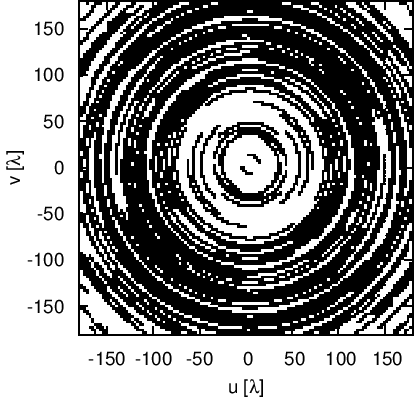
We assemble the interferometer array in a simple way by randomly placing 12 antennas and selecting all baseline pairs within the $uv$-plane. We then allow the assembly to rotate uniformly for 6 hours while observing the same sky patch at the north celestial pole. This choice of antenna arrangement and integration time roughly corresponds to existing instruments, such as an extended configuration of ALMA (Nyman et al. 2010) or VLA (Perley et al. 2011), although our fiducial setup uses fewer elements to highlight the performance of our method in less-than-optimal observing regimes. The interferometer pattern is discretized to the same resolution as our input images ($n_{p}=128$ pixels on a side; described below). We construct the interferometer pattern $I$ by placing a value of one wherever a baseline length intersects a pixel during its rotation and zeros elsewhere. We show the resulting $uv$-plane coverage in Figure 1. This configuration covers roughly $70\%$ of the $uv$-plane, although the coverage varies significantly for each $\ell$-bin, where $\ell$ is the radius of a given annulus in the $uv$-plane. Some bins, especially at very low and very high $\ell$, have zero coverage due to the lack of baselines at that distance. However, even if these bins had adequate coverage, we expect statistics here to be relatively poor due to the reduced number of modes in these regions. Most bins have at least $60\%$ coverage and several bins have complete coverage.

Figure 1: Fiducial interferometer pattern (black) after randomly placing 12 antennas and integrating for six hours assuming a pointing at the north celestial pole. The interferometer pattern is discretized to the same resolution as our input images ($n_{p}=128$ pixels on a side).

We determine the noise per pixel by summing the integration time spent in that pixel by all baselines. We do not adopt a noise model for a particular instrument; rather, we set the noise variance to be

$$\sigma_{i}^{2}\propto 1/t_{{\rm obs},i},$$ (2)

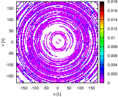
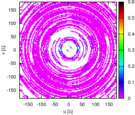
where $t_{\rm obs}$ is the observation time in pixel $i$. We then set an overall signal-to-noise ratio of $10$ by multiplying all noise variances by a constant value to maintain $|IFA~{}s|/|In|=10$. This provides a scaling of the noise that would normally be caused by instrument effects such as the effective area of the apertures and the system temperature in a realistic observation. We use a Gaussian realization of this noise variance to generate $n$ in Equation (1). We then multiply this noise by the interferometer pattern $I$ to maintain consistency with the signal. Figure 2 shows a particular noise realization for one of our test images and the resulting data $d$.

Figure 2: (left) Noise realization used in all test cases. The noise is randomly selected assuming a variance given by Eq. (2) and an overall signal-to-noise ratio of 10. (right) Example data $d$ (Equation 1) in the $uv$-plane for the Einstein test image.

2.2 Test Images

Radio interferometers are used to study a wide variety of interesting astrophysical and cosmological phenomena, such as supernova remnants (Bhatnagar et al. 2011), molecular gas clouds (Gratier et al. 2010), cluster radio halos (Cassano et al. 2010), magnetic fields in dwarf galaxies (Heesen et al. 2011), the interstellar medium (Zhang et al. 2012), the galactic center (McClure-Griffiths et al. 2012), and the cosmic microwave background (Pearson et al. 2005). To assess the ability of our method to cope with this variety of targets we select eight input images drawn from the CASA (Jaeger 2008) user guide , which we present in Figure 3.

Figure 3: Suite of test input images. All images have been rescaled to $128\times 128$ pixels and have had their intensities remapped to a maximum of unity. The repixelization process introduces some artefacts, which we leave in place to assess the ability of our isotropic prior to handle anisotropic data. Each image is 20 deg across. The color scale ranges from $0.0$ (black) to $1.0$ (white).

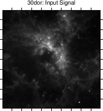
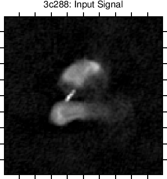
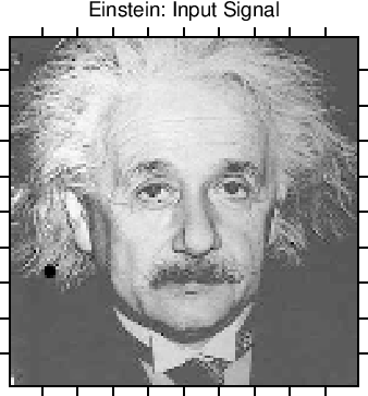
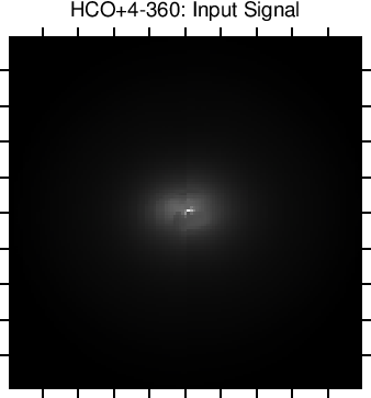
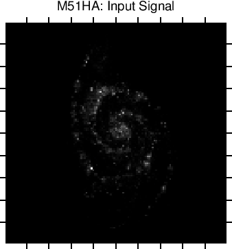
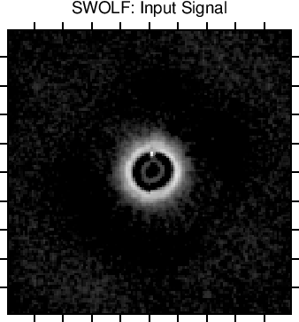
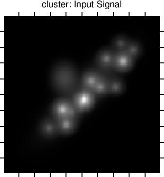
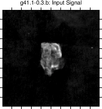
The test images represent a diverse variety of realistic — and a few unrealistic — imaging scenarios, such as a protoplanetary disk, a face-on spiral galaxy, a cluster, an AGN jet and lobe, and the face of Einstein. These images were provided in a mix of resolutions and dynamic ranges. To simplify our analysis (but without loss of generality), we remapped all images to a uniform grid $n_{p}=128$ pixels on a side and renormalized all intensities to a peak of unity. Some test images had artificial artefacts built-in, and the remapping procedure introduced some additional glitches in the image. We left these artefacts intact to test the ability of our isotropic Gaussian process prior to recover highly anisotropic portions of the data.

3 Method of Gibbs Sampling

Previous works have extensively discussed Gibbs Samples  (e.g., Wandelt et al. 2004; Sutter et al. 2012), so we only briefly introduce the relevant equations as applied to interferometric observations here. We begin with some initial guess of the angular power spectrum $C_{\ell}^{0}$ and progressively iterate samples from the conditional distributions

$$s^{i+1}\leftarrow P(s|C_{\ell}^{i},m)$$ (3)

$$C_{\ell}^{i+1}\leftarrow P(C_{\ell}|s^{i+1}),$$ (4)

where $m$ is the least squares estimate of the signal $s$ given the data $d$ (i.e., $B^{T}N^{-1}Bm=B^{T}N^{-1}d$, where $B$ represents a full signal-to-data operator). The samples $(C_{\ell}^{i},s^{i})$ converge to samples from the joint distribution $P(C_{\ell},s,m)=P(m|s)P(s|C_{\ell})P(C_{\ell})$ after a sufficient number of iterations.

Given an angular power spectrum sample $C_{\ell}^{i}$, we generate a new signal sample by drawing from a multivariate Gaussian with mean $S^{i}(S^{i}+N)^{-1}m$ and variance $((S^{i})^{-1}+N^{-1})^{-1}$. Here $S$ and $N$ are the signal and noise covariance, respectively. We do this by solving the set of equations

$$\begin{split}M~{}s^{i+1}=&~{}A^{T}F^{-1}I(INI)^{-1}d\\ &+F^{-1}S^{-1/2}F~{}\xi_{1}\\ &+A^{T}F^{-1}I(INI)^{-1/2}F~{}\xi_{2},\end{split}$$ (5)

where we define the matrix operator $M$ as

$$M\equiv F^{-1}S^{-1}F+A^{T}F^{-1}I(INI)^{-1}IFA.$$ (6)

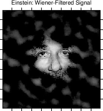
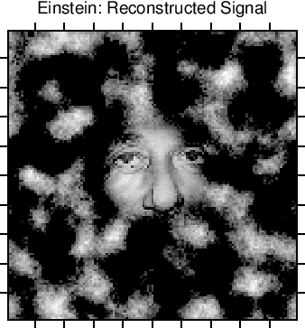
In the above equations $A^{T}$ is the primary beam transpose and $F^{-1}$ is the inverse Fourier transform. The first term in the right-hand side of the above equation provides the solution for the Wiener-filtered map, while the second and third terms of Eq. (5) provide random fluctuations with the required variance. The vectors $\xi_{1}$ and $\xi_{2}$ are of length $n_{p}$ with elements drawn from a standard normal distribution. As an illustration, Figure 4 shows an example Wiener-filtered map (i.e., from just solving the first term in the right-hand side) and full signal sample $s^{i}$ at a single iteration for the Einstein test case. We see that the fluctuation terms in Equation (5) fill in regions weakly constrained by the data with a guess that mimics the known portions of the signal given the level of noise.

Figure 4: Sample iteration of the Gibbs sampling algorithm for the Einstein test image, showing the Wiener-filtered signal (left) and full sample reconstruction with mock fluctuations added (right). Each image is 20 deg across. The color scale ranges from $0.0$ (black) to $1.0$ (white).

The signal covariance matrix $S$ is diagonal in the $uv$-plane for isotropic signals (which we assume as part of our Gaussian process prior), so $S_{\ell,\ell^{\prime}}=C_{\ell}\delta_{\ell,\ell^{\prime}}$, where $\ell=2\pi u$, with $u$ being the radial distance in the $uv$-plane. Here and throughout we assume the flat-sky approximation that makes this identity valid. By construction, Gibbs sampling explores the exact posterior and therefore treats the couplings introduced by partial sky coverage optimally (Wandelt et al. 2004). The algorithm “knows” about the couplings since they are contained in the data model (Eq. 1) which underlies the analysis. However, to a very good approximation the noise covariance matrix $N$ is diagonal, and thus we will assume this for simplicity. We assign to the matrix $N$ entries equal to $N_{i,j}=\sigma_{i}^{2}\delta_{i,j}$, where $\sigma_{i}$ is the noise variance for the $i$th pixel in the $uv$-plane. The construction $I(INI)^{-1}$ provides a pseudo-inverse of $N$, so that any locations in the $uv$-plane with no antenna coverage do not yield infinities when taking the inverse.

We solve numerically the above matrix-vector equation using a preconditioned conjugate-gradient scheme (Press et al. 1986). The preconditioner approximates the diagonal components of $M$ and is

$$P^{-1}=F^{-1}I(INI)^{-1}IF~{}(F^{-1}\tilde{A}^{2}),$$ (7)

where $\tilde{A}$ is the Fourier transform of the primary beam pattern. We implemented the code to solve the above equations with the open-source PETSc library  (Balay et al. 1997, 2010, 2011) and the MPI-parallelized version of FFTW (Frigo & Johnson 2005).

Given the latest signal sample, $s^{i}$, we generate a new angular power spectrum sample from Eq. (4) by computing the variance $\pi_{l}^{2}$ in annuli of constant $\ell$ on the Fourier-transformed signal. We then use this variance to draw from the probability density $P(C_{\ell}|s^{i})$, which follows an inverse Gamma distribution, by creating a vector $p_{\ell}$ of length $n_{\ell}$ (assuming a Jeffreys’ ignorance prior) and unit Gaussian random elements. Here, $n_{\ell}$ is the number of pixels in the bin $\ell$. The next power spectrum sample is then simply

$$C_{\ell}^{i+1}=\frac{\pi_{\ell}}{\left|p_{\ell}\right|^{2}}.$$ (8)

In the above, we assume $\ell(\ell+1)C_{\ell}$ to be constant across the width of each annulus in the $uv$-plane. The width of each annulus can be set as desired. For the test cases which we work with in this paper we chose the width to be $8\pi/L$, where $L$ is the longest baseline of the interferometer. This is four times the $uv$-space resolution. This choice limits correlations between angular power spectrum bins which develop as a consequence of partial sky coverage. All $\ell$-bins have uniform width except for the first, which we restrict to cover only the central zone where we enforce $C_{0}^{i}=0$, since our analysis cannot constrain the DC mode. We wish to capture as much power spectrum information as possible, so we correspondingly widen the width of the second bin to close this gap.

To determine convergence so that our iterative samples from the conditional distributions (Eq. 4) are indeed samples from the joint distribution, we employ multiple chains with different random number seeds. Our convergence criterion is the Gelman-Rubin (G-R) statistic, which compares the variance among chains to the variance within each chain. The G-R statistic asymptotes to unity, so convergence is said to be achieved when this statistic is below a given tolerance level for each $\ell$-bin (Gelman & Rubin 1992). For our test images we stopped iterating when the G-R statistic reached less than $1.1$, which took from 500 to 1500 steps, depending on the image.

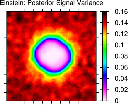
After convergence, we take the mean of the signal samples as our reconstructed image and simply calculate the variance for each pixel to assess the uncertainty in the reconstruction. Figure 5 shows the variance for the Einstein test image. We naturally see insignificant variance in the center of the primary beam where the data support is strongest, with steadily increasing variance away from the pointing center.

Figure 5: Posterior signal variance in image space (left) and acceptance mask derived from the variance (right) for the Einstein test image. The variance map is 20 deg across, and to show the detailed shape of the variance mask, we have zoomed in on the inner ten degrees. The acceptance region of the mask is shown in black.

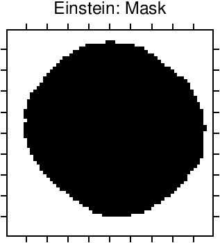
We may use the variance to build a mask of the final reconstructed image in which we only accept pixels below a given variance threshold. While this certainly isn’t necessary for the method to work, it provides an easy way to combine the posterior mean and variance information in a single plot. First, we compute the asymptotic variance $\sigma_{\rm asmp}$, or the mean of the variance along the outer edge of image plane. We then reject any pixel whose variance $\sigma$ is greater than $\sigma_{\rm asmp}/2$ and whose signal-to-noise ratio $s/\sqrt{\sigma}<1$. This last criterion prevents us from masking low-intensity, but still well-constrained, pixels. The values chosen to create the mask are arbitrary, and we choose them solely on aesthetic merit. We repeat: this mask is not necessary to perform the deconvolution and produce a reconstructed signal. We only use it to neatly incorporate the measured uncertainty information in the plotted images.

As we see in Figure 5, the acceptance mask generally follows the primary beam pattern. The detailed shape near the mask edge is influenced by the relative signal-to-noise levels and highlights the non-obvious nature of the regions of reliable reconstruction. We also notice an asymmetry in the acceptance mask: this is in response to the asymmetric nature of the fiducial interferometer setup (Figure 1) and provides strong evidence that the symmetric nature of our Gaussian process prior does not greatly influence our inference.

4 Comparison to CLEAN

We compare images recovered by Gibbs sampling, as described in the previous section, to those recovered by a proxy for the point source-based CLEAN algorithm. CLEAN is implemented in various radio interferometric imaging packages (such as CASA). However, it is not straightforward to use these packages to reconstruct images from simulated visibilities already defined on gridded coordinates; these packages are instead tailored to analyse observations made by real interferometric telescopes, with data in a specific format. Consequently, we compare to reconstructions made with a proxy for the point source-based CLEAN algorithm. While there are more sophisticated implementations of CLEAN that would undoubtedly perform better with our test images, this gives us a simple standard of comparison allowing us to demonstrate the viability of our method. We will include further comparisons in future work.

It was shown by Wiaux et al. (2009) that $\ell_{1}$ reconstruction with the Dirac basis (i.e. pixel basis) results in very similar reconstruction quality to CLEAN (see Wiaux et al. 2009; Figure 1). This is to be expected since it is known already that CLEAN is closely related to $\ell_{1}$ reconstruction with the Dirac basis (Marsh & Richardson 1987). We thus take a similar approach to that taken by recent studies (McEwen & Wiaux 2011; Carrillo et al. 2012; Wolz et al. 2013; Carrillo et al. 2013) and use $\ell_{1}$ reconstruction with a Dirac basis as a proxy for the CLEAN algorithm. The reconstructed image that serves as a CLEAN proxy is therefore given by the solution of the optimisation problem:

$$\min\|s\|_{1}\ \mbox{such that}\ \|d-IFAs\|_{2}\leq\epsilon\ ,$$ (9)

where $\|\cdot\|_{1}$ denotes the $\ell_{1}$ norm and $\epsilon$ is related to a residual noise level estimator (see, e.g., Wiaux et al. 2009; Carrillo et al. 2012). We solve this problem using the Sparse OPTimisation (SOPT) package (Carrillo et al. 2012; Carrillo et al. 2013) using the Douglas-Rachford splitting algorithm (Combettes & Pesquet 2007). Note that the SOPT package is a versatile code, capable of solving much more sophisticated optimisation problems than the straight-forward $\ell_{1}$ minimisation performed here (for examples of more extensive use see Carrillo et al. 2012, 2013b; Wolz et al. 2013).

Figures 6 and 7 are galleries of the input images (without noise), our posterior mean reconstruction using Gibbs sampling, and a standard reconstruction using our implementation of CLEAN. For all these images we have zoomed in to the inner 10 degrees where the primary beam selects the most prominent signal. We have applied our variance-based acceptance mask for our Gibbs sampling reconstructions. We see that Gibbs sampling is able to recover the complete range of source images to very high fidelity. We even faithfully recover glitches in the input image, such as the asymmetric protoplanetary disk in the SWOLF image and discontinuous lobe structure in the 3c288 image. This emphasizes the power of the Wiener Filter: in regions of strong data support, our samples are driven to the data regardless of choice of prior. We also recover low-intensity portions of the image both in the center of the image and towards the edge of the primary beam, such as the regions between the spiral arms in the M51HA image. However, there are other low-intensity regions, such as the lower portion of the mustache in the Einstein image, where the signal is too low to distinguish it from the noise, and our mask rejects those pixels.

Figure 6: Beamed input images without noise added ($As$; left column), posterior mean signal after 500 Gibbs sampling iterations (middle column), and CLEAN reconstruction (right column). Axes are marked in deg. For clarity we have zoomed in on the innermost 10 degrees where the signal is most prominent. The color scale ranges from $0.0$ (black) to $0.6$ (white).

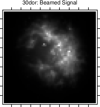
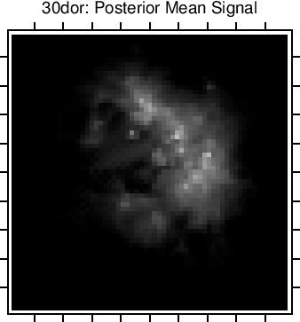
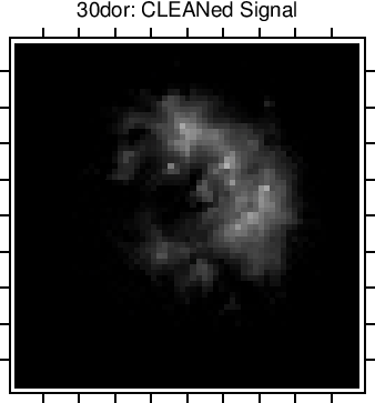
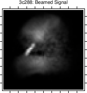
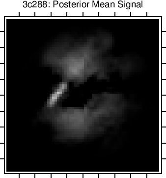
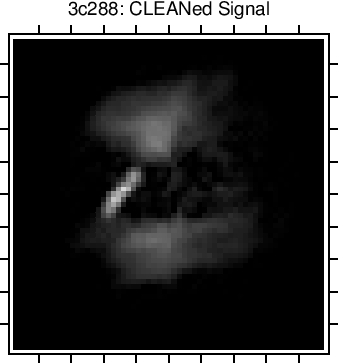
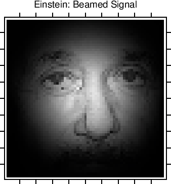
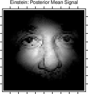
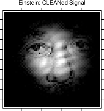
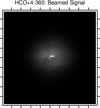
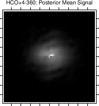
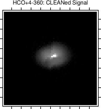
A comparison to the CLEAN images especially highlights the abilities of our Gibbs sampling reconstruction technique. In all images, we recover a broader range of fluxes over a wider extent than CLEAN (as in, for example, the cluster reconstruction). Also, Gibbs sampling is able to recover portions of the image further into the edges of the primary beam, as can be easily seen in the 3c288 and HCO+4-360 images. Finally, in images with glitches, such as SWOLF, CLEAN tends to exaggerate the asymmetries.

Figure 7: Same as Figure 6 for the remaining four test images.

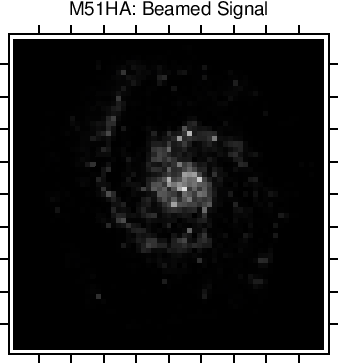
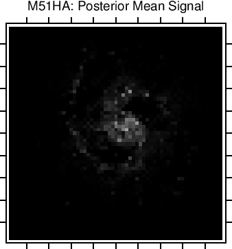
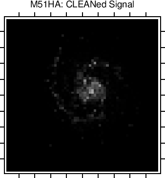
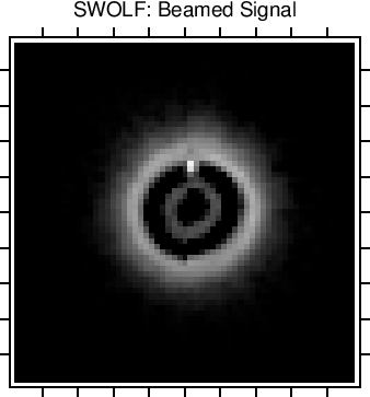
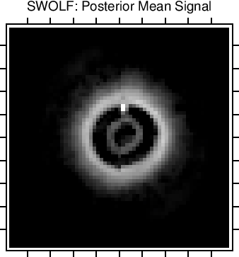
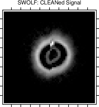
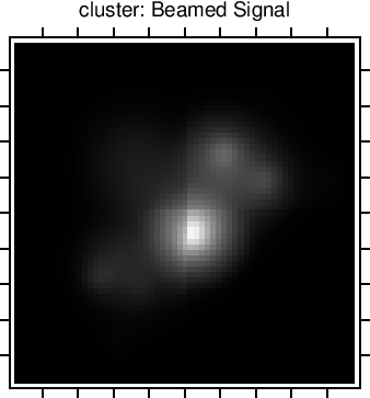
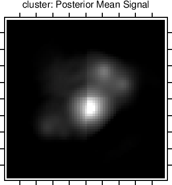
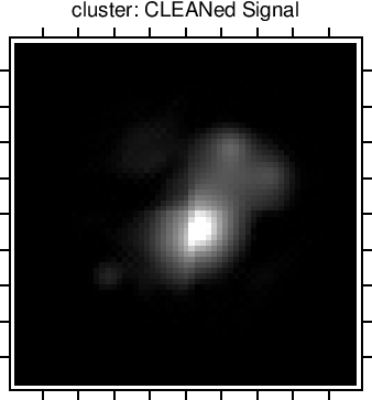
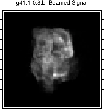
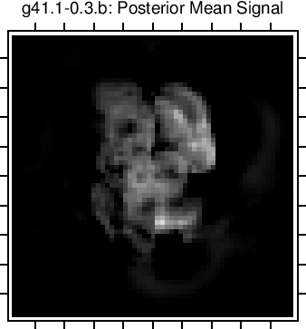
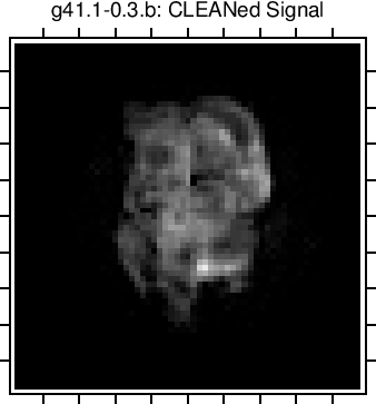
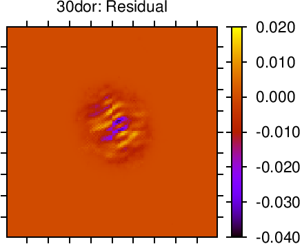
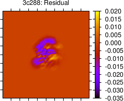
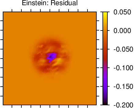
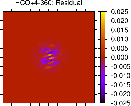
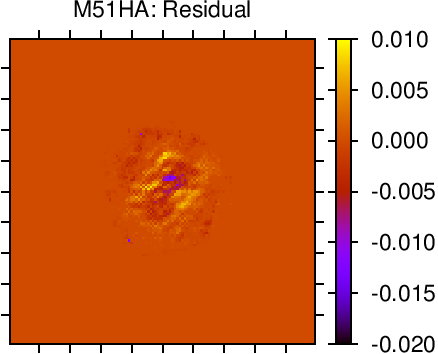
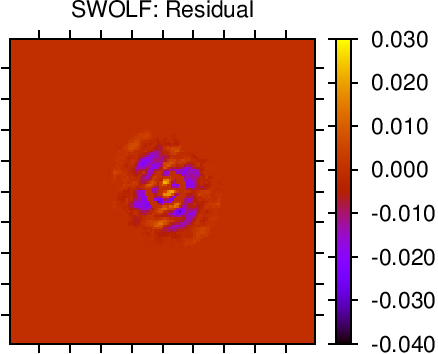
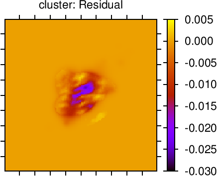
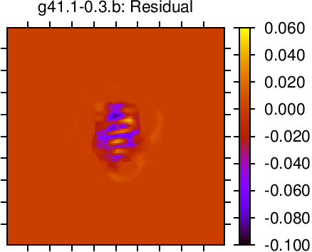
Figure 8 shows the residuals (i.e., difference maps) between the mean posterior signal generated by Gibbs sampling and the input test image. In all cases the variance-based acceptance mask has been applied. We see that the maximum residual occurs in the center of the Einstein test image, where the Gibbs method slightly underestimates the source intensity. This is probably due to the method attempting to average the very high-contrast features adjacent to the center. The Einstein image turns out to be the most difficult: the residuals for all other images are typically an order of magnitude smaller. While the residuals are somewhat correlated with the distributions of the source image, like the Einstein test image it appears that our method performs poorest in regions of high intensity contrast. However, these differences are very mild: typically on the order of 1% of the input source intensity.

Figure 8: Residuals (differences between reconstructed signal and beamed input signal $As$) for the Gibbs sampling algorithm for all test images. All images are 20 deg across. The color scale ranges from $0.0$ (black) to $1.0$ (white).

We may further quantify the differences between the input signals and their reconstructions with CLEAN and our Gibbs sampling method by binning the intensities, as we do in Figure 9. Bounding the histograms of the posterior mean are 2$\sigma$ error bars measured from the variance in the generated samples. This is another example of the kind of information unavailable in traditional reconstruction techniques. For almost all test images and intensity bins, our posterior mean reconstruction is within two standard deviations of the input signal. This is unsurprising: our Bayesian method automatically discovers the local variance because that variance is directly related to the relative level of signal and noise in a given bin. In a few bins, such as the high-intensity bin of the Einstein test image, our method tends to underestimate the true intensity. This is due to the high pixel-by-pixel contrast in the central image region discussed above.

Figure 9: Histograms of sky intensities in the beamed input signal $As$ (red), CLEAN reconstructed sky (green), and Gibbs sampling reconstructed sky (blue). Error bars (light blue) on the Gibbs sampling intensities are 2$\sigma$ uncertainties calculated from the posterior signal samples.

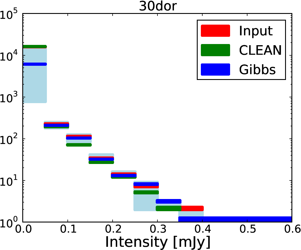
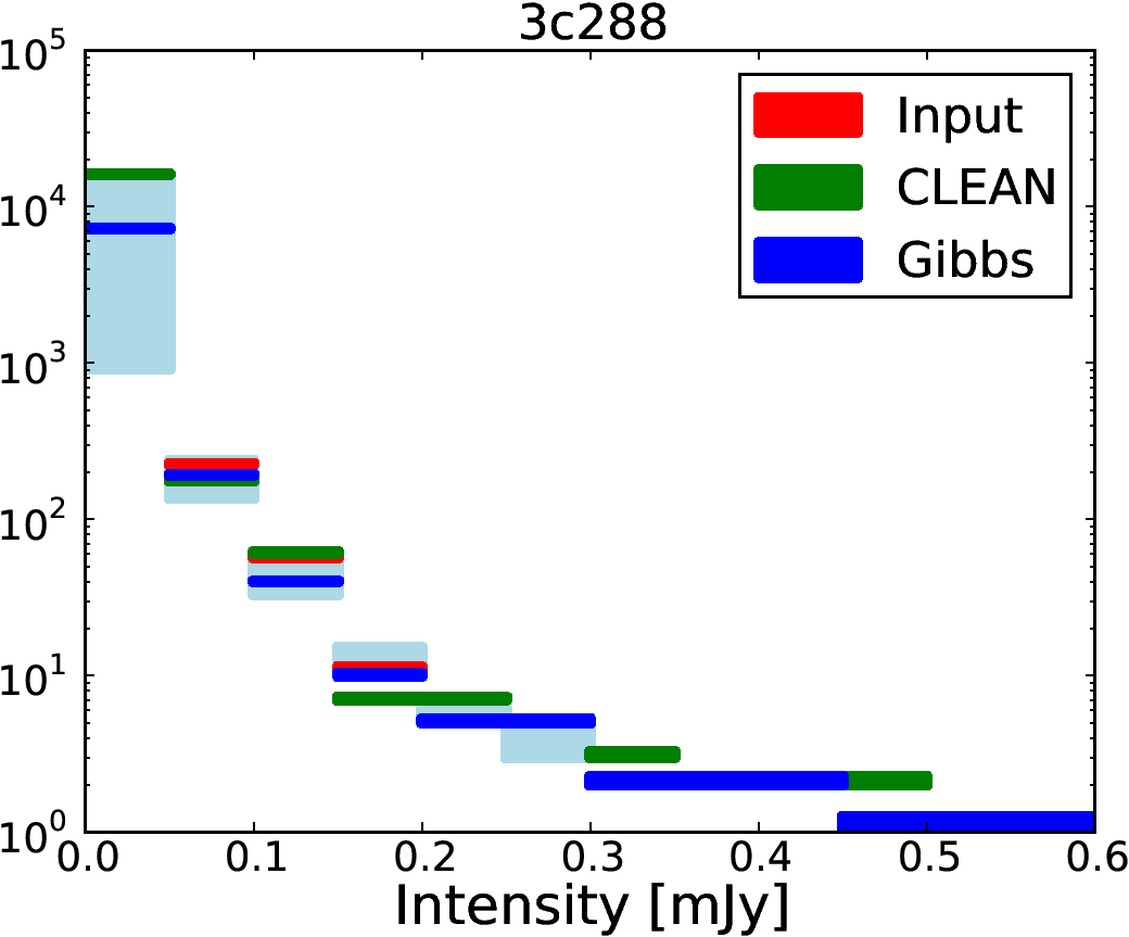
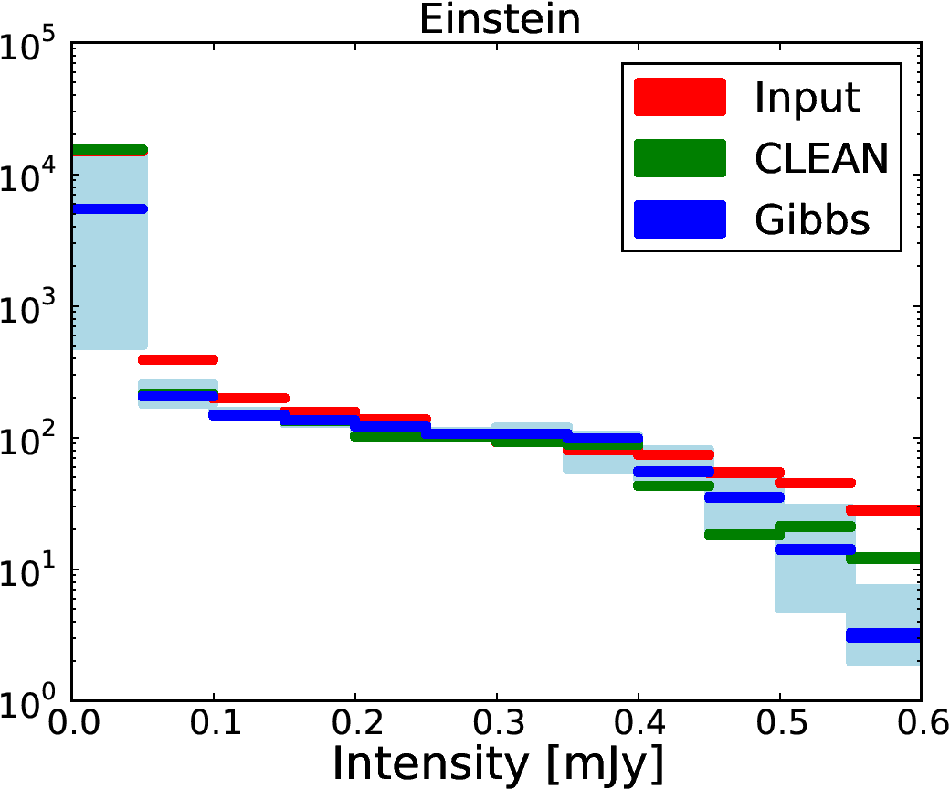
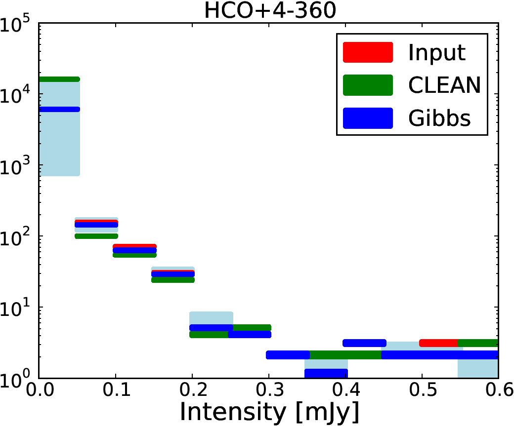
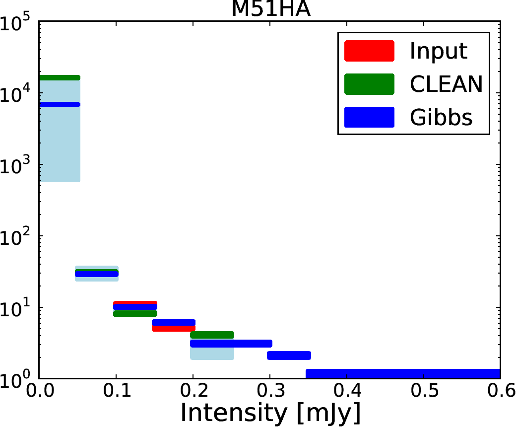
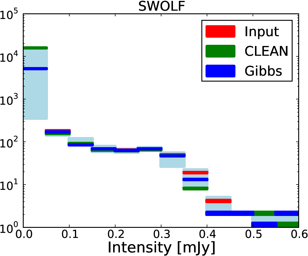
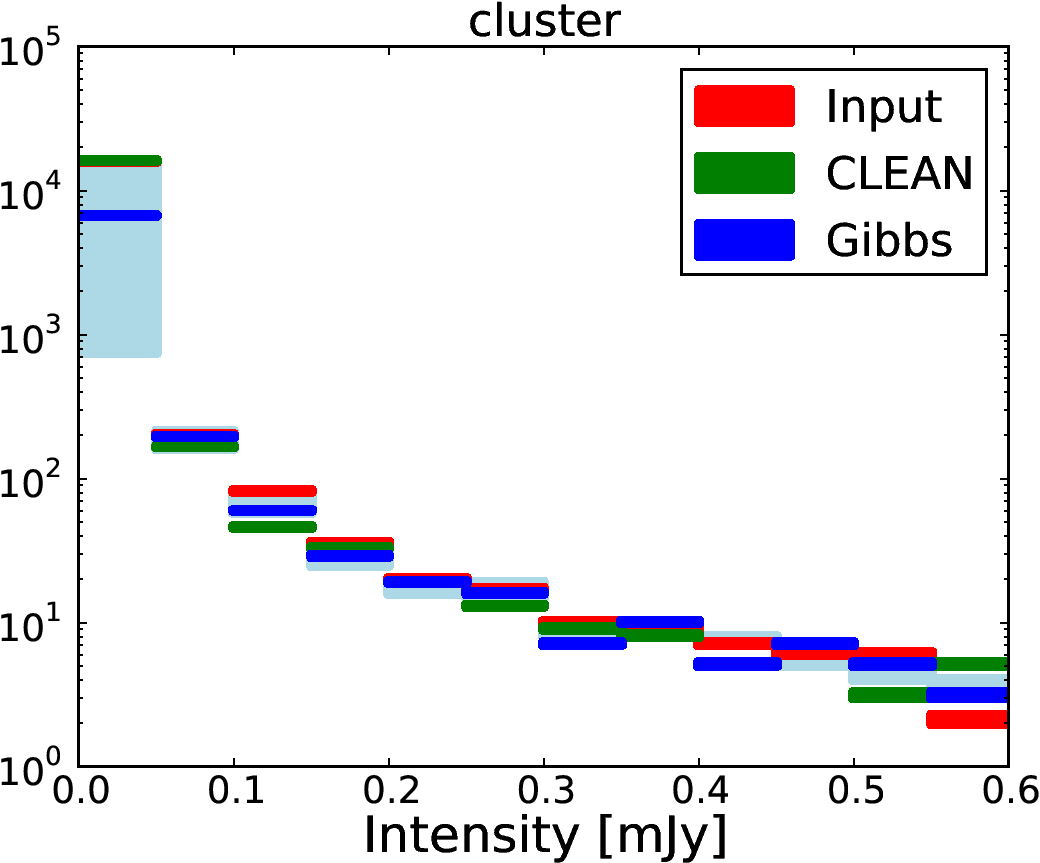
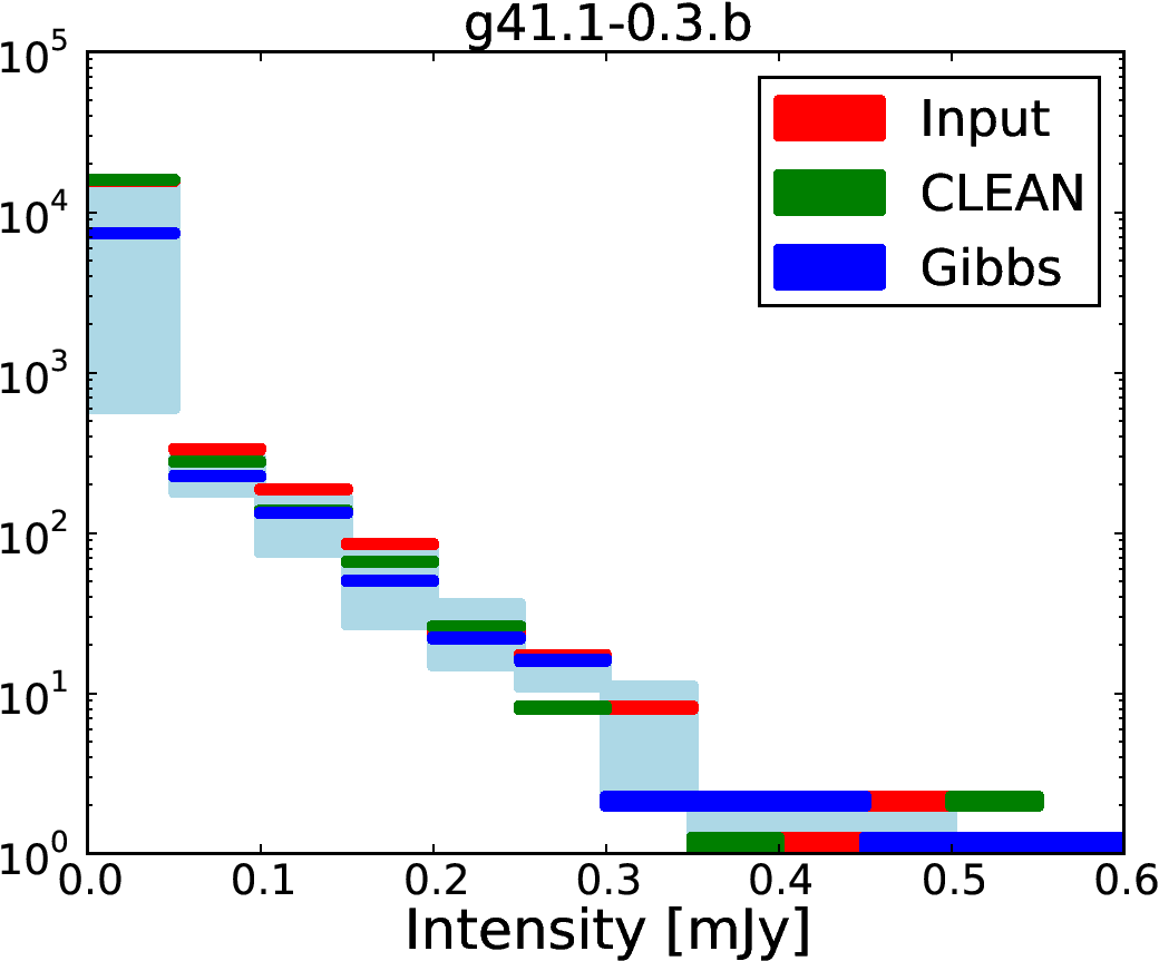
While the CLEAN image intensities largely fall within the uncertainty ranges of the Gibbs reconstruction, there is a systematic steepening of the distributions: CLEAN tends to have too many low-intensity pixels and correspondingly too many high-intensity pixels. This validates the discussion above which noted that CLEAN does not fully reproduce the observed range of input fluxes.

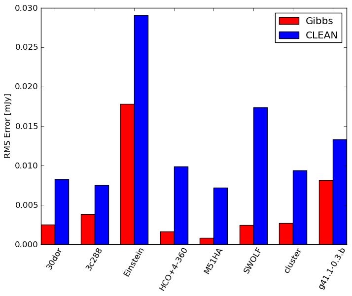
Finally, we may further simplify the comparison by reducing our measurement error to a single scalar. Two error metrics are commonly used: the root-mean-square (RMS) of the residual map, and the signal-to-noise ratio (SNR). This last quantity itself has several variations; we take that of Carrillo et al. (2012):

$${\rm SNR}\equiv 20\log_{10}\frac{\sigma_{s}}{\sigma_{s-\hat{s}}},$$ (10)

where $\sigma_{x}$ is the standard deviation of image x, with $s$ denoting the original image and $\hat{s}$ denoting the reconstructed image. For both measures we first apply our variance-based acceptance mask before calculating the error metrics.

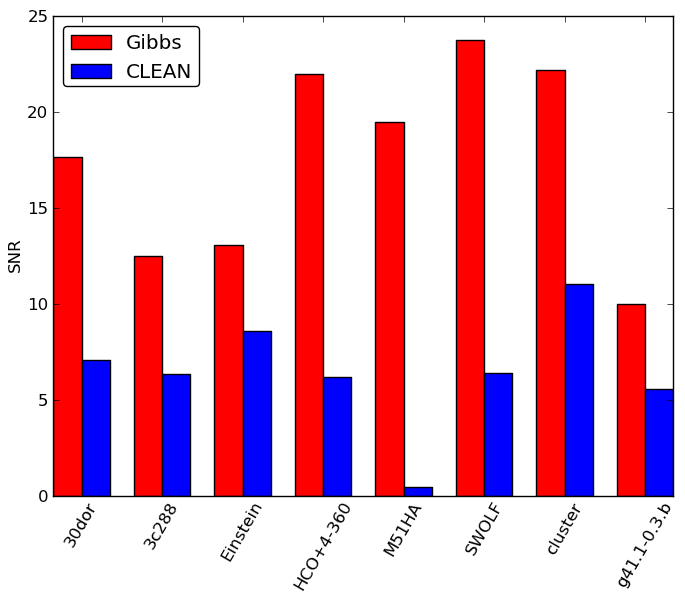
Figure 10 shows the RMS and SNR for each of our test images for both Gibbs sampling and traditional CLEAN. As expected from our residuals, Gibbs sampling performed most poorly in terms of RMS with the Einstein test image due to its highly complex structure. With the exception of that image and g41.1-0.3.b, all RMS errors are below $4\times 10^{-3}$. The SNR for all reconstructions with Gibbs sampling fall between 10 and 25. In both RMS and SNR measures Gibbs sampling outperforms CLEAN for all test images. The largest differences occur in images with high degrees of symmetry (e.g., M51HA, SWOLF) since in these cases our isotropic Gaussian process prior performs best in marginal signal-to-noise portions of the image.

Figure 10: Quantitative assessment of the errors. We show RMS error between the beamed input signal $As$ and the reconstructed images in the left plot. In the right plot we show the SNR as defined by Eq. (10). For each image we compare the Gibbs sampling reconstructed sky (red) to the CLEAN reconstruction (blue). For the RMS (SNR) error measurement, smaller (larger) values indicate better performance.

5 Conclusions

We have presented an innovative method for deconvolving radio interferometric images using the Bayesian method of Gibbs sampling. Our method naturally offers several advantages over traditional deconvolution approaches. It fully accounts for signal and noise mode coupling and incomplete $uv$-plane coverage in an automatic and well-motivated fashion, requires no fine-tuning or supervision as the method progresses, and provides an informative description of the uncertainty information in the signal reconstruction. We choose an isotropic Gaussian process image prior, though we don’t specify the signal covariance in advance.

We have tested our method with a realistic interferometric observing scenario of a wide variety of source images. These images represent typical targets, including protoplanetary disks and active galactic nuclei jet-and-lobe systems. Note that our choice of prior is wrong for all test cases, but the iterative application of the Wiener filter allows us to discover the source images within the noise and incomplete $uv$-plane coverage. We find that our method is quite robust: regardless of the structure of the source image we are able to recover the intensity distribution to a very high fidelity. Our method outperforms traditional point source-based CLEAN in terms of intensity distributions, RMS error, and reconstruction signal-to-noise ratio. As expected given our isotropic Gaussian process prior, we perform best on images with large amount of symmetry, though the Wiener filter provides a route for reliable reconstructions of asymmetric images in regions of strong data support regardless of source structure.

Using our method we can also easily incorporate uncertainty information in the reconstructed image. As discussed in earlier works (Wandelt et al. 2004), the error model generated from the isotropic Gaussian process prior tends to underestimate the true errors, but this situation is far preferable to no error model at all. With our error model we can construct acceptance masks based on the local (i.e., pixel-by-pixel) signal-to-variance ratios. The desired threshold can be adjusted based on the desired level of confidence in the deconvolution. Since the sample variance is directly tied to the relative level of noise by way of the Wiener Filter, our method naturally and self-consistently determines this mask.

While the test cases we have presented in this work use an interferometric setup with realistic noise levels, primary beam shape, and antenna array, they do represent a relatively simplistic observing scenario. A fully implemented method would include simultaneous solutions of multiple frequencies, mosaicked images, and wide bandwidth observations. Also, we have specified an overall SNR of 10 for our fiducial observations, and we must examine the performance of this method in different regimes.

Additionally, future large-scale interferometers will deliver incredibly high volumes of data. Image deconvolution from even a single pointing at a single frequency will tax most computing systems. To accommodate future data sets we have implemented our algorithm using the MPI-parallelized PETSc (Balay et al. 2011) toolkit, so our approach automatically grows with the size of the data without loss of scalability. Algorithmically, the most expensive portion of our approach is the solution to Equation (5), which scales as $\mathcal{O}(n_{p}\log n_{p})$ in the ideal pregridded flat-sky approximation we have presented here.

While we have not discussed foreground removal in this work, this method easily accommodates modeling in two fashions. First, partial signal or foreground information, if known in advance, can enter as an additional prior. Alternatively, foreground models can be added as an additional sampling step within the algorithm (Wandelt et al. 2004). The resulting posterior mean signal will thus automatically include marginalizations over the unconstrained parameters of the model. The same approach can be taken with the noise: if, for example, the noise spectrum is known but the absolute amplitude is not, we can sample over that amplitude. This flexibility, in addition to the other strengths discussed above, suggest that Gibbs sampling is a promising response to the challenges of contemporary and future radio interferometric observations.

References

- Ables (1974) Ables J. G., 1974, Astron. & Astrophys. Suppl., 15, 383
- Ayasso et al. (2012) Ayasso H., Rodet T., Abergel A., 2012, Inverse Problems, 28, 125005
- Balay et al. (2010) Balay S., et al., 2010, Technical Report ANL-95/11 - Revision 3.1, PETSc Users Manual. Argonne National Laboratory
- Balay et al. (2011) Balay S., et al.,, 2011, PETSc Web page http://www.mcs.anl.gov/petsc
- Balay et al. (1997) Balay S., Gropp W. D., McInnes L. C., Smith B. F., 1997, in Arge E., Bruaset A. M., Langtangen H. P., eds, Modern Software Tools in Scientific Computing Efficient Management of Parallelism in Object Oriented Numerical Software Libraries. Birkh{ä}user Press, pp 163–202
- Baron et al. (2012) Baron F., et al., 2012, in Society of Photo-Optical Instrumentation Engineers (SPIE) Conference Series Vol. 8445 of Society of Photo-Optical Instrumentation Engineers (SPIE) Conference Series, The 2012 interferometric imaging beauty contest
- Bhatnagar (2009) Bhatnagar S., 2009, in Saikia D. J., Green D. A., Gupta Y., Venturi T., eds, The Low-Frequency Radio Universe Vol. 407 of Astronomical Society of the Pacific Conference Series, Calibration and Imaging Challenges at Low Radio Frequencies: A Review of the State of the Art. p. 375
- Bhatnagar & Cornwell (2004) Bhatnagar S., Cornwell T. J., 2004, Astron. & Astrophys., 426, 747
- Bhatnagar et al. (2011) Bhatnagar S., Rau U., Green D. A., Rupen M. P., 2011, ApJ, 739, L20
- Carrillo et al. (2013) Carrillo R. E., McEwen J. D., Ville D. V. D., Thiran J.-P., Wiaux Y., 2013, IEEE Sig. Proc. Let., 20, 591
- Carrillo et al. (2012) Carrillo R. E., McEwen J. D., Wiaux Y., 2012, Mon. Not. Roy. Astron. Soc., 426, 1223
- Carrillo et al. (2013) Carrillo R. E., McEwen J. D., Wiaux Y., 2013, submitted to Mon. Not. Roy. Astron. Soc., arXiv:1307.4370
- Cassano et al. (2010) Cassano R., Brunetti G., Röttgering H. J. A., Brüggen M., 2010, Astron. & Astrophys., 509, A68
- Combettes & Pesquet (2007) Combettes P., Pesquet J.-C., 2007, IEEE J. Selected Top. in Sig. Proc., 1, 564
- Cornwell (2008) Cornwell T. J., 2008, IEEE Journal of Selected Topics in Signal Processing, 2, 793
- Cornwell & Evans (1985) Cornwell T. J., Evans K. F., 1985, Astron. & Astrophys., 143, 77
- Frigo & Johnson (2005) Frigo M., Johnson S., 2005, Proceedings of the IEEE, 93, 216
- Gelman et al. (2004) Gelman A., Carlin J., Stern H., Rubin D., 2004, Bayesian Data Analysis. Chapman & Hall/CRC
- Gelman & Rubin (1992) Gelman A., Rubin D., 1992, Statistical Science, 7, 457
- Giovannelli & Coulais (2005) Giovannelli J.-F., Coulais A., 2005, Astron. & Astrophys., 439, 401
- Gratier et al. (2010) Gratier P., et al., 2010, Astron. & Astrophys., 522, A3
- Gull & Daniell (1978) Gull S. F., Daniell G. J., 1978, Nature, 272, 686
- Heesen et al. (2011) Heesen V., Rau U., Rupen M. P., Brinks E., Hunter D. A., 2011, ApJ, 739, L23
- Högbom (1974) Högbom J. A., 1974, Astron. & Astrophys. Suppl., 15, 417
- Jaeger (2008) Jaeger S., 2008, in Argyle R. W., Bunclark P. S., Lewis J. R., eds, Astronomical Data Analysis Software and Systems XVII Vol. 394 of Astronomical Society of the Pacific Conference Series, The Common Astronomy Software Application (CASA). p. 623
- Jarvis (2007) Jarvis M. J., 2007, At the Edge of the Universe: Latest Results from the Deepest Astronomical Surveys ASP Conference Series, Vol. 380, proceedings of the conference held 9-13 October, 2006 at Sintra, Portugal. Edited by José Afonso, Henry C. Ferguson, Bahram Mobasher, and Ray Norris., p.251, 380
- Jewell et al. (2004) Jewell J., Levin S., Anderson C. H., 2004, ApJ, 609, 1
- Johnston et al. (2008) Johnston S., et al., 2008, Experimental Astronomy, 22, 151
- Li et al. (2011) Li F., Cornwell T. J., de Hoog F., 2011, Astron. & Astrophys., 528, A31
- Lonsdale et al. (2009) Lonsdale C. J., et al., 2009, Proceedings of the IEEE, 97, 1497
- McEwen & Wiaux (2011) McEwen J. D., Wiaux Y., 2011, Mon. Not. Roy. Astron. Soc., 413, 1318
- Mackay (2003) Mackay D. J. C., 2003, Information Theory, Inference and Learning Algorithms. Cambridge University Press
- Marsh & Richardson (1987) Marsh K. A., Richardson J. M., 1987, Astron. & Astrophys., 182, 174
- McClure-Griffiths et al. (2012) McClure-Griffiths N. M., Dickey J. M., Gaensler B. M., Green A. J., Green J. A., Haverkorn M., 2012, Astrophys. J. Supp., 199, 12
- Myers et al. (2003) Myers S. T., et al., 2003, ApJ, 591, 575
- Norris et al. (2013) Norris R. P., et al., 2013, ”Radio Continuum Surveys with Square Kilometre Array Pathfinders”, Pub. of the Astro. Soc. of Aus., 30, 20
- Nyman et al. (2010) Nyman L.-Å., Andreani P., Hibbard J., Okumura S. K., 2010, in Society of Photo-Optical Instrumentation Engineers (SPIE) Conference Series Vol. 7737 of Society of Photo-Optical Instrumentation Engineers (SPIE) Conference Series, ALMA science operations
- Parsons et al. (2010) Parsons A. R., Backer D. C., Foster G. S., Wright M. C. H., Bradley R. F., Gugliucci N. E., Parashare C. R., Benoit E. E., Aguirre J. E., Jacobs D. C., Carilli C. L., Herne D., Lynch M. J., Manley J. R., Werthimer D. J., 2010, AJ, 139, 1468
- Pearson et al. (2005) Pearson T. J., et al., 2005, New Cosmological Data and the Values of the Fundamental Parameters, Proceedings of IAU Symposium 201, held 7-11 August 2000 at Manchester, United Kingdom. Edited by A. Lasenby and A. Wilkinson. San Francisco, CA: Astronomical Society of the Pacific (ASP)
- Perley et al. (2011) Perley R. A., Chandler C. J., Butler B. J., Wrobel J. M., 2011, ApJ, 739, L1
- Press et al. (1986) Press W. H., Flannery, Brian P. Teukolsky, Saul A. 1986, Numerical recipes. The art of scientific computing, Cambridge: University Press
- Puetter et al. (2005) Puetter R. C., Gosnell T. R., Yahil A., 2005, Annual Review of Astronomy and Astrophysics , 43, 139
- Rau (2012) Rau U., 2012, in Society of Photo-Optical Instrumentation Engineers (SPIE) Conference Series Vol. 8500 of Society of Photo-Optical Instrumentation Engineers (SPIE) Conference Series, Radio interferometric imaging of spatial structure that varies with time and frequency
- Rau & Cornwell (2011) Rau U., Cornwell T. J., 2011, Astron. & Astrophys., 532, A71
- Starck et al. (2001) Starck J.-L., Murtagh F., Querre P., Bonnarel F., 2001, Astron. & Astrophys., 368, 730
- Stewart et al. (2011) Stewart I. M., Fenech D. M., Muxlow T. W. B., 2011, Astron. & Astrophys., 535, A81
- Suksmono (2009) Suksmono A., 2009, in ICEEI Vol. 1, Deconvolution of vlbi images based on compressive sensing. pp 110–116
- Sutter et al. (2012) Sutter P. M., Wandelt B. D., Malu S. S., 2012, Astrophys. J. Supp., 202, 9
- Sutton & Wandelt (2006) Sutton E. C., Wandelt B. D., 2006, Astrophys. J. Supp., 162, 401
- Thompson et al. (2001) Thompson A. R., Moran J. M., Swenson George W. J., 2001, Interferometry and synthesis in radio astronomy by A. Richard Thompson, New York
- Wandelt et al. (2004) Wandelt B., Larson D., Lakshminarayanan A., 2004, Phys. Rev. D, 70, 12
- Wenger et al. (2010) Wenger S., Magnor M., Pihlström Y., Bhatnagar S., Rau U., 2010, Publications of the Astronomical Society of the Pacific (PASP), 122, 1367
- Wiaux et al. (2009) Wiaux Y., Jacques L., Puy G., Scaife A. M. M., Vandergheynst P., 2009, Mon. Not. Roy. Astron. Soc., 395, 1733
- Wiaux et al. (2010) Wiaux Y., Puy G., Vandergheynst P., 2010, Mon. Not. Roy. Astron. Soc., 402, 2626
- Wolz et al. (2013) Wolz L., McEwen J. D., Abdallah F. B., Carrillo R. E., Wiaux Y., 2013, Mon. Not. R. Astron. Soc., 436, 1993
- Zhang et al. (2012) Zhang H.-X., Hunter D. A., Elmegreen B. G., 2012, ApJ, 754, 29