The Gemini NICI Planet-Finding Campaign:
The Frequency of Planets around Young Moving Group Stars

Abstract

We report results of a direct imaging survey for giant planets around 80 members of the $\beta$ Pic, TW Hya, Tucana-Horologium, AB Dor, and Hercules-Lyra moving groups, observed as part of the Gemini NICI Planet-Finding Campaign. For this sample, we obtained median contrasts of $\Delta$$H$=13.9 mag at 1” in combined CH₄ narrowband ADI+SDI mode and median contrasts of $\Delta$$H$=15.1 mag at 2” in $H$-band ADI mode. We found numerous ($>$70) candidate companions in our survey images. Some of these candidates were rejected as common-proper motion companions using archival data; we reobserved with NICI all other candidates that lay within 400 AU of the star and were not in dense stellar fields. The vast majority of candidate companions were confirmed as background objects from archival observations and/or dedicated NICI campaign followup. Four co-moving companions of brown dwarf or stellar mass were discovered in this moving group sample: PZ Tel B (36$\pm$6 M_Jup, 16.4$\pm$1.0 AU, Biller et al. 2010) , CD -35 2722B (31$\pm$8 M_Jup, 67$\pm$4 AU, Wahhaj et al. 2011), HD 12894B (0.46$\pm$0.08 M_⊙, 15.7$\pm$1.0 AU), and BD+07 1919C (0.20$\pm$0.03 M_⊙, 12.5$\pm$1.4 AU). From a Bayesian analysis of the achieved H band ADI and ASDI contrasts, using power-law models of planet distributions and hot-start evolutionary models, we restrict the frequency of 1–20 M_Jup companions at semi-major axes from 10–150 AU to $<$18% at a 95.4$\%$ confidence level using DUSTY models and to $<$6% at a 95.4$\%$ using COND models. Our results strongly constrain the frequency of planets within semi-major axes of 50 AU as well. We restrict the frequency of 1–20 M_Jup companions at semi-major axes from 10–50 AU to $<$21% at a 95.4$\%$ confidence level using DUSTY models and to $<$7% at a 95.4$\%$ using COND models. This survey is the deepest search to date for giant planets around young moving group stars.

1 Introduction

In the last decade, $\sim$10 planets and planet candidates with estimated masses $<$13 M_Jup have been imaged in orbit around young stars and brown dwarfs (e.g. Chauvin et al., 2005a; Marois et al., 2008; Kalas et al., 2008; Lafrenière et al., 2008; Lagrange et al., 2009, 2010; Marois et al., 2010; Todorov et al., 2010; Ireland et al., 2011; Luhman et al., 2011; Kraus & Ireland, 2012; Rameau et al., 2013; Quanz et al., 2013; Kuzuhara et al., 2013; Bowler et al., 2013). In total, $\sim$30 companions with estimated masses $<$25 M_Jup have been imaged. (See http:$//$exoplanet.eu for a compilation of these objects.) These discoveries have provided a wealth of new information about young giant planets, as well as some surprises. Prior to these detections, models predicted that young gas giant planets at moving group ages (10-300 Myr) would likely have cool photospheres with prominent methane absorption features (Baraffe et al., 2003; Burrows et al., 2003), i.e. that these objects would be spectral analogs to T-type brown dwarfs. However, all known directly-imaged planets at these ages (specifically 2MASS 1207b and the HR 8799 planets, Chauvin et al., 2005a; Marois et al., 2008, 2010) have lacked methane absorption and show extremely red colors, likely due to dust clouds and/or non-equilibrium chemistry in their atmospheres (Bowler et al., 2010; Skemer et al., 2011; Barman et al., 2011a, b; Currie et al., 2011).

Additionally, all of these companions except for $\beta$ Pic b (Lagrange et al., 2009, 2010), HR 8799e (Marois et al., 2010), and LkCa 15b (Kraus & Ireland, 2012) lie at projected separations greater than 20 AU, considerably wider than giant planets in our own solar system. Such widely separated companions pose a challenge for the accepted model of core-accretion formation, which likely formed the closer-in ($<$10 AU) population of planets detected to date via radial velocity studies (e.g.,  Mordasini et al., 2009; Janson et al., 2012; Dodson-Robinson et al., 2009). However, given that only $\sim$10 such companions have been imaged to date, it is perhaps premature to make statements based on such a small sample. Thus, it is a priority to discover additional companions as well as to constrain on the distributions of their semimajor axes, eccentricities, masses, etc.

In the last decade, a number of deep, adaptive-optics aided surveys with sample sizes $>$20 stars have been completed at 8-m telescopes to search for additional planetary companions. Many of these have been conducted in the 1.6 $\mu$m $H$-band or 2.2 $\mu$m $K$-band (Masciadri et al., 2005; Biller et al., 2007; Lafrenière et al., 2007b; Apai et al., 2008; Chauvin et al., 2010), while others have focused further into the infrared (3.5-5 $\mu$m) in the $L$, $L^{\prime}$, or $M$ bands (Kasper et al., 2007; Heinze et al., 2010a, b; Rameau et al., 2013a). A number of very large scale surveys ($>$100 stars) are ongoing or recently completed, including the NICI Campaign at Gemini-South (Liu et al. 2010, this publication, Wahhaj et al. 2013a, Nielsen et al. 2013, Wahhaj et al. 2013b), the NACO large program using NACO at the VLT (Buenzli et al. 2010), SEEDS (Strategic Exploration of Exoplanets and Disks with Subaru) using HiCIAO at Subaru (Thalmann et al., 2009; Carson et al., 2013), and the International Deep Planet Survey (IDPS) using primarily Gemini and Keck (Vigan et al., 2012).

The host stars of currently known directly-imaged planets fall into three categories: (1) members of young ($\lesssim$10 Myr) star-forming clusters or OB associations (e.g. Taurus and Upper Sco; Lafrenière et al., 2008; Todorov et al., 2010; Kraus & Ireland, 2012) , (2) members of nearby young moving groups (ages of 10–300 Myr, e.g. Lagrange et al., 2010; Chauvin et al., 2005a; Marois et al., 2008), and (3) unassociated nearby young stars (e.g. Kalas et al., 2008). Of these three categories of targets, moving group objects are particularly compelling targets for direct imaging searches. The extremely young ages of star-forming clusters translates into considerably brighter planets, but at distances $\geq$140 pc the inner working angles of current instruments generally only allow detection of companions at projected separations $\gtrsim$50 AU. Unassociated nearby young stars often do not have well constrained ages, a limitation for estimating the mass of any companion detected and for deriving statistics for the survey sensitivities. Moving group stars provide a unique nearby young sample with well-constrained ages and distances.

We have observed 80 young moving group stars as a part of a dedicated science campaign using the Near-Infrared Coronagraphic Imager (NICI) at the 8.1 m Gemini South Telescope (Chun et al., 2008). NICI is a dedicated adaptive optics (AO) instrument tailored expressly for direct imaging of exoplanet companions, combining several techniques to attenuate starlight and suppress speckles for direct detection of faint companions to bright stars: (1) Lyot coronagraphy, (2) dual-channel imaging for Spectral Differential Imaging (SDI; Racine et al., 1999; Marois et al., 2005; Biller et al., 2007), and (3) operation in a fixed Cassegrain rotator mode for Angular Differential Imaging (ADI; Liu, 2004; Marois et al., 2006; Lafrenière et al., 2007a; Biller et al., 2008). While each of these techniques has been used individually in large planet-finding surveys (e.g.  Biller et al., 2007; Lafrenière et al., 2007b), the NICI Campaign is the first time all three have been employed simultaneously in a large survey.

From 2008 December to 2012 September, the NICI Planet-Finding Campaign (Liu et al., 2010) obtained deep, high-contrast AO imaging of a carefully selected sample of over 200 young, nearby stars. Over the course of the Campaign, we discovered 4 new brown dwarf companions to young stars: PZ Tel B (Biller et al., 2010), CD -35 2722B (Wahhaj et al., 2011), HD 1160C (Nielsen et al., 2012), and HIP 79797Bab (Nielsen et al., 2013). Here we report results from the subsample of 80 young stars that are members of the $\beta$ Pic, TW Hya, AB Dor, Tucana-Horologium, and Hercules-Lyra moving groups.

2 Moving Group Sample

Moving groups are associations of young stars (10–300 Myr) that are unconnected to regions of ongoing star-formation. These associations were not discovered until the late 1990’s, as moving group members are often dispersed across a wide part of the sky (e.g.  Zuckerman & Song, 2004; Torres et al., 2008). Moving group members are identified by a combination of youth indicators (Li absorption, high X-ray luminosity, etc.) and space motion coincident with other cluster members. We have focused our survey on 5 young moving groups with members generally within $\sim$60 pc of the Earth.

2.1 TW Hya Association

The star TW Hya was the first pre-main sequence (henceforth PMS) star identified outside of a star-forming region, initially identified by Rucinski & Krautter (1983) as an isolated T Tauri star. de la Reza et al. (1989) and Gregorio-Hetem et al. (1992) identified 4 additional T Tauri stars within 10 degrees of TW Hya. Kastner et al. (1997) were the first to label these stars as the TW Hya Association, based on their strong lithium absorption features, X-ray fluxes, and similar Hipparcos parallaxes. Since then, $>$20 TW Hya members have been identified (see  Webb et al., 1999; Sterzik et al., 1999; Jayawardhana et al., 1999; Zuckerman et al., 2001a; Gizis, 2002; Song et al., 2002, 2003; Kastner et al., 2008; Zuckerman et al., 2004; Scholz et al., 2005; Mamajek, 2005; Looper et al., 2007; Torres et al., 2008; Fernández et al., 2008; da Silva et al., 2009; Looper et al., 2010a, b; Rodriguez et al., 2011; Shkolnik et al., 2011). Based on lithium absorption and X-ray flux strength, the association is assigned an age of $\approx$10 Myr (Kastner et al., 1997; Webb et al., 1999). The mean distance of the TW Hya association is 48$\pm$13 pc (Torres et al., 2008; Weinberger et al., 2013).

2.2 $\beta$ Pic Moving Group

The circumstellar disk around the nearby A star $\beta$ Pic was first imaged by Smith & Terrile (1984), leading to the identification of $\beta$ Pic as a young star with planet formation having occurred in the recent past. Barrado y Navascués et al. (1999) found two additional M type stars (GJ 799 and GJ 803) with matching Galactic space motions to $\beta$ Pic. Zuckerman et al. (2001b) cemented the existence of the $\beta$ Pic moving group with the confirmation of 18 additional members on the basis of their Galactic space motions. Over 60 members of the $\beta$ Pic moving group have been identified to date (Song et al., 2003; Zuckerman & Song, 2004; Torres et al., 2006, 2008; Fernández et al., 2008; da Silva et al., 2009; Lépine & Simon, 2009; Rice et al., 2010; Schlieder et al., 2010; Kiss et al., 2011; Schlieder et al., 2012; Shkolnik et al., 2012). From the color-magnitude diagram placement of these stars as well as their lithium absorption ages, an age of $\approx$12 Myr is estimated for this moving group (Zuckerman & Song, 2004), with a mean distance of 31$\pm$21 pc (Torres et al., 2008).

2.3 Tucana-Horologium Association

Young stars are often far-IR excess sources. Based on this fact, Zuckerman & Webb (2000) searched the Hipparcos catalog for stars with similar space motions and within a 6 degree radius of 24 stars detected at 60 $\mu$m with IRAS. From this search, they identified $\sim$10 stars with distances of $\sim$45 pc and ages of $\sim$30 yr, which they named the Tucana Association. Torres et al. (2000) found a group of $\sim$10 stars through X-ray emission and ground-based spectroscopy that showed youth indicators and are associated with the previously identified isolated T Tauri star EP Eri, which they titled the Horologium Association. As the stars in these two associations share the same space motions, ages, distances, and volume density, they are now considered to be part of the same association (Zuckerman et al., 2001c). Over 60 stars have been identified to date in the Tucana-Horologium association (Song et al., 2003; Zuckerman & Song, 2004; Torres et al., 2008; Fernández et al., 2008; da Silva et al., 2009; Kiss et al., 2011; Zuckerman et al., 2011), with a mean distance of 48$\pm$7 pc (Torres et al., 2008).

2.4 AB Dor Moving Group

The star AB Dor is notable as an ultrafast rotator which is also extremely X-ray active, at a distance of only 15 pc and an age of $\sim$100 Myr (Luhman et al., 2005). AB Dor itself, in fact, is a quadruple system with a close M-dwarf companion and a wider separation M-dwarf binary (Guirado et al., 1997; Close et al., 2005; Nielsen et al., 2005; Close et al., 2007). Zuckerman et al. (2004) identified $\sim$30 nearby star systems with similar space motions to AB Dor as well characteristics of youth, which they designated the AB Dor moving group. Over 50 stars have been identified to date in the AB Dor moving group (Zuckerman & Song, 2004; Torres et al., 2008; Fernández et al., 2008; da Silva et al., 2009; Schlieder et al., 2010; Zuckerman et al., 2011; Schlieder et al., 2012; Shkolnik et al., 2012), with a mean distance of 34$\pm$26 pc (Torres et al., 2008).

2.5 Hercules-Lyra Association

Gaidos (1998) first identified 4 young solar analogues with similar space motions towards Hercules. Fuhrmann (2004) identified a further 15 late-type stars with similar space motions and gave the whole complex the name Hercules-Lyra. The existence of the Hercules-Lyra association was initially disputed, as the candidate members possessed a wide age spread inconsistent with a single moving group, with some of the initially identified stars possessing ages (derived from lithium absorption and chromospheric activity) much younger or older than the average association age of $\sim$200 Myr. López-Santiago et al. (2006) confirmed the existence of the Hercules-Lyra association and winnowed down the 27 initial candidate members to 10 confirmed members with an average distance of 20$\pm$10 pc and age of $\sim$200 Myr.

3 Observations

We observed 80 stars in nearby young moving groups as part of the NICI Campaign – 14 stars from the TW Hya association, 30 stars from the $\beta$ Pic moving group, 12 stars from the Tucana-Horologium association, 19 stars from the AB Dor moving group, 4 stars from the Hercules-Lyra association, and 1 star (BD +1 2447) which is either a Hercules-Lyra or AB Dor moving group member. The survey sample was selected from a larger sample of moving group stars compiled from the literature. Observations were prioritized according to the probability of detecting a planet around a given survey star (Liu et al., 2010), as predicted by Monte Carlo simulations similar to those described in Section 5.1.

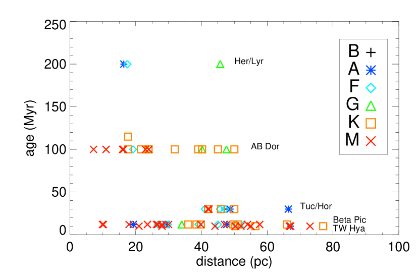
Figure 1: NICI Campaign moving group sample plotted as a function of distance and age. Plot symbols give object spectral type and each moving group is labeled at the appropriate age. The majority (85$\%$) of stars in our sample have ages less than 100 Myr and distances less than 60 pc. We observed 14 stars from the TW Hya association, 30 stars from the $\beta$ Pic moving group, 12 stars from the Tucana-Horologium association, 19 stars from the AB Dor moving group. 4 stars from the Hercules-Lyra association, and 1 star (BD +1 2447) which is either a Hercules-Lyra or AB Dor moving group member.

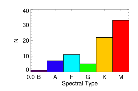
Figure 2: Histograms of the spectral types and distances of our 80 MG sample objects. Column width is 1 spectral type and 10 pc respectively. The median distance for this sample is 39.8 pc. We observed 1 B star, 7 A stars, 11 F stars, 5 G stars, 23 K stars, and 33 M stars. About 70$\%$ of our sample have spectral types of K or later; thus, our sample is comprised largely of lower mass stars.

The survey sample is listed in Table LABEL:tab:properties and is plotted as a function of age, distance, and spectral type in Figure 1. Histograms of the spectral type and distance distributions are presented in Figure 2. The majority (85$\%$) of sample stars have ages less than 100 Myr and distances less than 60 pc. The median distance is 39.8 pc. We observed 1 B star, 7 A stars, 11 F stars, 5 G stars, 23 K stars, and 33 M stars. Thus, our moving group sample is primarily composed of lower mass stars. Observations of our survey sample are listed in Table 2. We only report observations which contain at least 10 individual images in the ADI or ASDI sequences, in order to achieve the field rotation needed by our ADI processing pipeline to obtain reliable detections (see Section 3.2 for details).

3.1 The Near-Infrared Coronagraphic Imager at Gemini South

NICI was specifically designed to provide the high contrasts necessary to directly image young extrasolar giant planet. NICI’s 85-element curvature AO system provides AO correction of $\sim$30-45$\%$ Strehl in $H$ band (Chun et al., 2008). The AO beam is then reflected into the science camera, where it passes through a partially transparent focal plane mask. The focal plane mask is a flat-topped Gaussian, which suppresses $>$99.5$\%$ of the incoming starlight ($\Delta$CH_4S=6.39$\pm$0.03 mag, $\Delta$$H$=5.94$\pm$0.05 mag; Wahhaj et al., 2011), thus reducing scattered light from the central star and increasing the attained contrast. A variety of these semi-transparent masks are available for use with NICI; we utilized the 0.32$\arcsec$ radius mask for NICI Campaign observations, thus providing an effective inner working angle of 0.32$\arcsec$ for faint companions, although tight stellar companions can still be detected in the innermost regions. The partially-transparent mask also allows us to attain very precise photometry and astrometry, as we can simultaneously obtain unsaturated images of both the primary and faint companions. The beam then passes through a hard-edged pupil stop, which reduces diffracted light from PSF artifacts associated with the Gemini-South secondary mirror. For observations in dual-channel mode, the beam is split using a dichroic and passes into two separate science cameras. For the majority of the Campaign, a 50/50 beamsplitter was utilized, resulting in the loss of half of the incoming light to each channel, but from the beginning of 2012, this beamsplitter was replaced by an H/K dichroic, boosting throughput when imaging simultaneously in these two filters. Different filters may be chosen for each science camera; thus NICI’s 2-camera capability can provide simultaneous color information. Both cameras have fields of view of 18$\times$18$\arcsec$, with a platescale of 17.96 mas for the science camera using the 1.578 $\mu$m $CH_{4}S$ filter (henceforth ”blue channel” or ”off-methane channel”) and a platescale of 17.94 for the science camera using the 1.652 $\mu$m $CH_{4}L$ 4% filter (henceforth ”red channel” or ”on-methane channel”) for the science camera using the 1.578 $\mu$m.

3.2 Observing Strategy 

NICI Campaign observations were conducted in two separate modes: (1) single channel H-band ADI (Angular Differential Imaging) mode and (2) dual-channel methane band combined ADI+SDI (Spectral Differential Imaging) mode. Both SDI and ADI techniques seek to distinguish real objects from speckles. SDI achieves this by exploiting a spectral feature in the desired target (e.g. the 1.6 $\mu$m methane absorption feature observed in substellar objects with a T spectral type Geballe et al., 2002; Cushing et al., 2005). Images are taken simultaneously both within and outside the chosen absorption feature. Due to the simultaneity of the observations, the stellar point-spread functions in the two NICI channels, including the coherent speckle patterns, are nearly identical. In contrast, any faint companion with the chosen absorption feature is bright in one filter and faint in the other. Subtracting the two images thus removes the starlight and speckle patterns while a real companion with the chosen absorption feature remains in the image. In other words, the absorption band image acts as an ideal reference point spread function (henceforth PSF) for the off-absorption band image. Utilizing a signature spectral feature of substellar objects can help distinguish between true methanated companions and likely background objects, e.g. a background object will be subtracted out by the SDI subtraction since it will not have methane absorption. However, this mode is sensitive even to companions without this absorption feature, as a real companion will appear fixed in separation relative to the star in both filters, while a speckle will modulate with the Airy pattern and appear further from the star in the red filter relative to the blue filter.

ADI employs a different strategy in order to decorrelate real companions from speckles. For ADI observations, the rotator is left off at the Cassegrain focus or set to follow the elevation angle at the Nasmyth focus, allowing the telescope optics rotate relative to the sky. In a sequence of images taken at different parallactic angles, a real companion will move relative to the detector along with the sky, while the speckles will remain fixed. From a series of images, a reference PSF can thus be constructed for and subtracted from each individual image, attenuating quasi-static speckle structure. Combining both SDI and ADI techniques (henceforth ASDI) thus allows an even greater degree of speckle supression.

In order to take advantage of both the higher contrast available within 1.5” using the ASDI mode (due to improved speckle suppression from the SDI subtraction) and the improved sensitivity available outside of 1.5” with the ADI mode (due to the wider bandpass used during our ADI observations), most NICI Campaign stars were observed in both modes. For ASDI mode, we observed simultaneously in the off-methane (central $\lambda$=1.578 $\mu$m; width=0.062 $\mu$m; $CH_{4}S$ 4%) and on-methane (central $\lambda$=1.652 $\mu$m; width=0.066 $\mu$m; $CH_{4}L$ 4%) bands using NICI’s dual-channel imaging capability. ADI data were taken with the broadband $H$ filter in the blue channel (central $\lambda$=1.65 $\mu$m, width=0.29 $\mu$m) Stars fainter than $H$=8 mag were observed only in single-channel ADI mode, as the contrast within 1.5” was similar to that achievable in the ASDI mode. Stars close to the Galactic Bulge were only observed in ASDI mode, as ADI mode often yielded enormous numbers ($>$50 per field) of background field objects.

Typically, we obtained 20 minutes on-sky data in ADI mode and 40 minutes on-sky data in ASDI mode for each star. Observations were carefully scheduled in order to maximize field rotation while avoiding too much blurring during single exposures. We aimed to obtain at least 5^∘ field rotation in ADI mode observations and at least 15^∘ field rotation in ASDI mode observations. This ensures on-sky rotations of at least 3$\times$FWHM of the PSF at 5” separation from the primary in ADI mode and at least 3$\times$FWHM of the PSF at 1” separation in ASDI mode. Typical FWHMs of the PSF ranged between 3-4 pixels. Out of 68 stars with ADI mode observations, all but 4 have at least one dataset with sky rotation $>$5 degrees. Out of 56 stars with ASDI observations, all but 7 have at least one dataset with sky rotation $>$15 degrees, and only one ASDI observation has sky rotation $<$10 degrees.

For ASDI, individual exposure times were chosen to produce high S/N in the speckle halo while avoiding saturation in this region. In ADI mode, exposure times of 4 to 60 s were used, allowing the halo to saturate if needed. For bright stars that saturate in the ADI exposures, short exposures were interleaved with deep exposures in order to provide unsaturated images of the star behind the partially transparent mask (henceforth the “starspot”) for accurate photometry.

3.3 Data Reduction

All observations are processed using a custom pipeline described in Wahhaj et al. (2013b). Here we briefly summarize procedures for both ADI and ASDI datasets; some data processing steps pertain only to the ASDI mode and are noted as such below. For all data, the pipeline first applies dark, flatfield, and distortion corrections. For ADI data, all images are centroided and aligned to the first exposure in the sequence. For ASDI data, images from the two science cameras are then centroided and aligned. Datasets where the starspot is unsaturated are aligned using the starspot centroid position in each science exposure. For saturated images, the structure of the saturated PSF is used to align the images (Wahhaj et al., 2013b). Specifically, the peak of the primary is still discernible as a negative image and can be used to centroid. We have estimated that the centroiding accuracy of the saturated images is 9 mas by comparing these to the centroids of unsaturated short-exposure images obtained right before and after the long exposures. Image filters (i.e. unsharp masking or catch filtering) are applied frame-by-frame. In the ASDI case, the red-channel image is subtracted from the blue-channel image for each science exposure. A high-fidelity PSF is built for the entire observation by median combining the stack of reduced images and then subtracted from each individual science exposure. Finally, the reduced PSF-subtracted images are registered, rotated to a common sky orientation, and stacked to produce a final image. In the ASDI case, 3 final output images are produced: the full subtracted reduction as well as single-channel ADI reductions for the blue and red channel images respectively, which can be added to achieve deeper sensitivity. This ensures that no planet candidates are missed due to spectral self-subtraction in the ASDI mode.

4 Results

4.1 Contrast Curves and Minimum Detectable Masses

In order to robustly measure the contrast achieved by our pipeline reductions, we generate 95%-completeness contrast curves following the method described in Wahhaj et al. (2013b). The 95%-completeness technique accounts for self-subtraction losses endemic to ADI and SDI data, unlike simple measurements based solely on the noise level of the data. Briefly, the data are first pipeline-processed, rotationally misaligned (derotated in the opposite direction of the actual parallactic angle rotation), and stacked to create a companion-free reduction. The 1$\sigma$ contrast curve is calculated from the standard deviation found in 3 pixel annuli as a function of separation from the primary star. Next, a set of 20$\sigma$ simulated companions (1340 total simulated companions, at separations of 0.36$\arcsec$ to 6.3$\arcsec$ and uniformly distributed in azimuth in 67 concentric rings), produced by scaling the image of the primary star behind the partially-transparent mask, is inserted into the individual raw images, and the new data are re-reduced as before. The 20$\sigma$ simulated companions are recovered in the reduced data and used to evaluate the flux losses and artifacts in input contrasts due to the pipeline. Finally, the recovered companions (now with flux loss effects and other pipeline artifacts incorporated) are reinserted into the original reduction and scaled in intensity until they meet our detection criteria. The contrast at which 95% of the simulated companions are detected is presented as the 95%-completeness contrast curve.

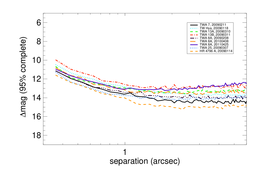
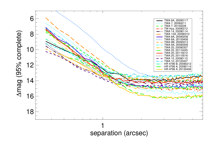
Figure 3: 95% completeness contrast curves for TW Hya association stars, with plot range from 0.3” (coronagraph inner working angle) to 6”. A contrast of 15 magnitudes represents a flux ratio of 10⁶. Top: ASDI contrasts. Bottom: ADI contrasts.

The 95% completeness contrast curves for the moving group sample are presented in Figures 3 to 8. Tables of measured contrast are presented for the ASDI subtracted reductions in Table 3 and for the ADI reductions in Table 4.

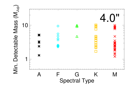
Figure 9: Minimum detectable masses as a function of spectral type at 0.5$\arcsec$, 1$\arcsec$, 2$\arcsec$, and 4$\arcsec$, using the DUSTY models of Baraffe et al. (2002) to convert from contrasts to masses. At 0.5$\arcsec$ we are sensitive to companions of $\leq$13 M_Jup for all but one star. At 2$\arcsec$ we are sensitive to companions with masses $<$10 M_Jup for all stars. The minimum detectable mass varies by star (according to spectral type, magnitude, distance, etc.) but we are generally sensitive to $\geq$5 M_Jup companions at 2$\arcsec$. around all sample stars.

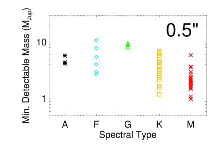
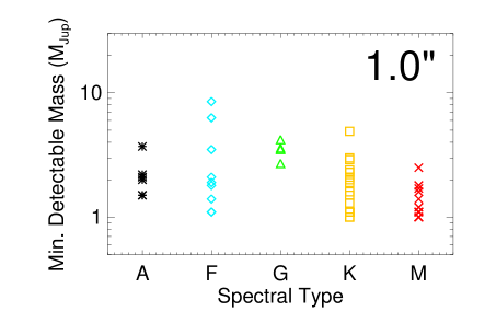
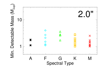
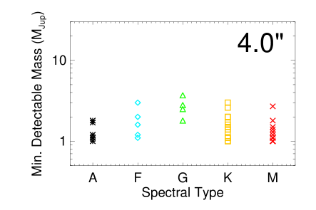
Figure 10: Minimum detectable masses as a function of spectral type at 0.5$\arcsec$, 1$\arcsec$, 2$\arcsec$, and 4$\arcsec$, using the COND models of Baraffe et al. (2003) to convert from contrasts to masses. At 0.5$\arcsec$ we are sensitive to companions of $\leq$10 M_Jup for all but one star. At 2$\arcsec$ we are sensitive to companions with masses $<$5 M_Jup for all stars. The minimum detectable mass varies by star (according to spectral type, magnitude, distance, etc.) but we are generally sensitive to $\geq$5 M_Jup companions at 2$\arcsec$ around all sample stars.

For our ADI contrast curves, we convert measured contrast to maximum detectable apparent magnitude in Table 5 and minimum detectable mass in Tables 6 and Tables 7. We interpolated from both the DUSTY and COND models of Chabrier et al. (2000) and Baraffe et al. (2002, 2003) using the maximum detectable apparent magnitudes, distance, and age of each stars to estimate the minimum detectable mass curves. At some point as they cool and dust condenses from their atmospheres, directly imaged exoplanets are predicted to transition from red, dusty L dwarf spectra (DUSTY) to T dwarf spectra with methane absorption features (COND). However, no directly imaged planet to date has yet to show strong methane absorption in the near-IR, with only weak methane absorption observed at longer wavelengths (Skemer et al., 2012). Thus as this transition has not been observed, we choose here to present minimum detectable masses according to both of these models. Minimum detectable masses as a function of spectral type at 0.5$\arcsec$, 1$\arcsec$, 2$\arcsec$, and 4$\arcsec$ are presented in Figure 9 using the DUSTY models (Baraffe et al., 2002) and in Figure 10 using the COND models (Baraffe et al., 2003). For the more conservative DUSTY model case, at 0.5$\arcsec$ we are sensitive to companions of $\leq$13 M_Jup for all but one star. At 2$\arcsec$ we are sensitive to companions with masses $\leq$10 M_Jup for all stars. The minimum detectable mass varies by star (according to spectral type, magnitude, distance, etc.) but we are generally sensitive to $\geq$5 M_Jup companions at 2$\arcsec$ around all sample stars. We do not present minimum detectable masses in ASDI subtracted mode here, as this requires knowledge of a potential companion’s $H$-band spectrum. For an example of such an analysis of ADI self-subtraction as a function of radius, see Nielsen et al. (2013).

4.2 Astrometry of Candidate Companions

We found numerous candidate companions in our images. Candidates were first identified using an automated finding algorithm and then verified by eye. For the entire NICI Campaign sample, candidate companions were found for $\sim$50$\%$ of observed stars. The vast majority of these objects are not expected to be true co-moving companions. To test whether a candidate companion is co-moving with its parent star requires reobserving after enough time has elapsed for significant proper motion and/or parallactic motion of the star in the sky, ideally at the $\geq$3 pixel ($\geq$50 mas) or greater level.

After identifying candidate companions in our reduced images, we first checked if any older archival data from VLT, HST or Gemini were available. In this manner, we were able to immediately identify a number of bright candidates as background objects. Astrometry for candidates observed at multiple epochs with NICI as well as other telescopes is presented in Tables 8 and 9.

For objects with HST NICMOS observations, we retrieved data from the HST MAST archive and used the mosaic files. Images taken at different telescope roll angles were subtracted to remove the slowly changing speckle pattern (henceforth roll subtraction). For datasets with images taken at only one roll angle, images were rotated by 180^∘ and subtracted from themselves. We typically performed roll subtraction without any subpixel alignment as most of the candidates were well outside the region where PSF subtraction was important. Lowrance et al. (2005) found the position of the star behind the NICMOS coronagraph using acquistion images and slew vectors gleaned from HST engineering telemetry, and claim that the difference image diffraction spikes do not give an accurate measure of the star’s position. Our candidate companions followed up with NICMOS archival data are generally at wide separations ($>$2”) and with large time baselines (usually $\geq$3 years) relative to the NICI epoch; thus, we often did not require an extremely accurate knowledge of the central star position in order to determine if they were background objects. To see if the simpler method of using the diffraction spikes could be used, we tested this method on 10 stars in the Lowrance et al. (2005) sample by measuring the position of the same companions they reported. We found a mean difference of 1.2 pixels from their positions. Taking this to be entirely due to our centroiding method, we combine it in quadrature with their reported 1.05 pixel (0.08”) uncertainty to calculate a total uncertainty of 1.6 pixels, or 0.12”.

Data from Gemini-NIRI were reduced using a custom ADI script (Close & Males, 2010). Due to saturation of the primary stars, we estimate our astrometric uncertainty to be $\sim$2 pixels, or 0.044”.

Candidates within 400 AU from the star and not in dense stellar fields that were not confirmed or rejected as common-proper motion companions using archival data were reobserved with NICI. NICI astrometry was measured relative to the unsaturated starspot position in either the science or short exposures. The uncertainties in the separation and PA are estimated to be 0.009″(0.5 pixel) and 0.2^∘ respectively, when the primary is unsaturated, and 0.018″(1 pixel) and 0.5^∘ when the primary is saturated (Wahhaj et al. 2013b).

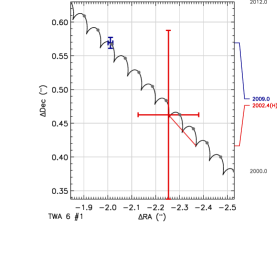
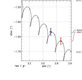
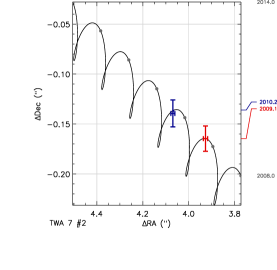
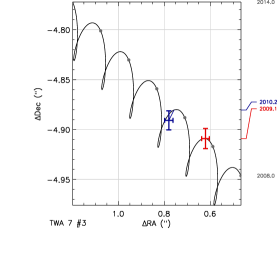
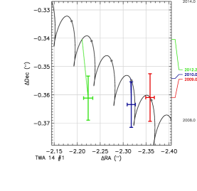
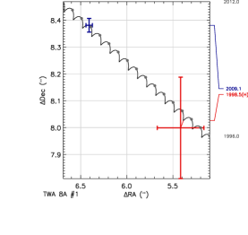
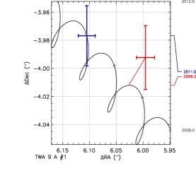
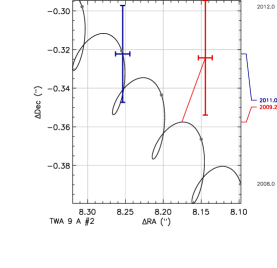
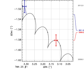
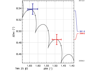
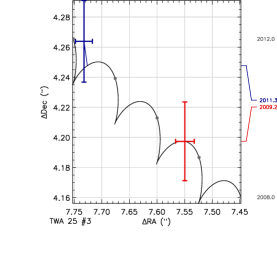
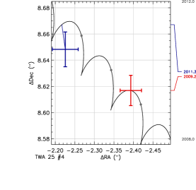
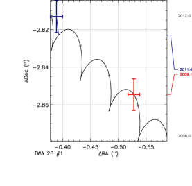
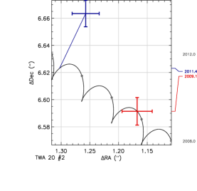
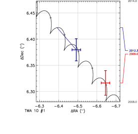
Figure 11: On-sky plots for TW Hya association objects. For each candidate, the background track (black curve) is calculated from the proper motion and parallax of the star and position of the candidate at the initial reference epoch. Astrometry at the reference epoch and additional epochs are shown as points with error bars, and a colored line (1st epoch red, 2nd epoch blue, 3rd epoch green) connects the position at additional epochs to the expected position on the background track. The labels at the right of each plot give the epochs of each astrometric data point, at the vertical position corresponding to the location on the background track for that epoch. When the epoch is given alone, the observation was conducted with the NICI instrument. Otherwise observational data are taken from VLT NACO (V), Keck NIRC2 (K), VLT ISAAC (I), ESO 3.6m (E), and Gemini NIRI (G).

From the proper motions and parallaxes of our MG sample stars and pinning to the NICI first epoch position, we can calculate the expected motion relative to the primary star for each candidate companion, assuming that the candidate is a background object. On-sky plots presenting background ephemerides and the actual on-sky motion of each candidate companion relative to the primary are presented in Figures 11 to 15. We compute the $\chi^{2}$ value for the expected background track position relative to the actual sky position for each candidate (see Nielsen et al. 2013). $\chi^{2}$ values are shown in Table 8. Candidates with reduced $\chi^{2}$ values close to 1 are confirmed to be background objects. In total, 81 candidate companions were tested for common proper motion with either archival or 2nd epoch Gemini NICI data. Of these candidates, 77 were background objects; however, four co-moving brown dwarf or stellar companions (discussed in more detail in Section 7) were detected for the first time in the moving group sample: PZ Tel B (Biller et al., 2010), CD -35 2722B (Wahhaj et al., 2011), HD 12894B (this work) and BD+07 1919C (this work). We also retrieve the known stellar companion to HD 82688 (Metchev & Hillenbrand, 2009), as well as the brown dwarf companions AB Pic B (Chauvin et al., 2005b) and HR 7329B (Lowrance et al., 2000; Guenther et al., 2001).

A number of stars (HD 139084 B, V343 Nor, CD-54 7336, CD-31 16041, HD 159911, GJ 560 A, and TYC 7443-1102-1) were near the Galactic Bulge and often possessed extremely dense starfields ($>$20 objects in the NICI images). As we expect almost all of these candidates to be background objects, we assigned these stars lower priority for second epoch NICI followup and consequently they were not observed before the end of the NICI Campaign. Astrometry for candidates observed at only one epoch and thus unconfirmed as background or common proper motion is presented in Table 17.

4.3 New Stellar Binaries

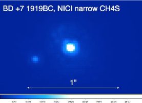
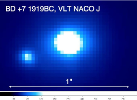
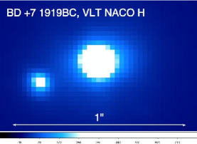
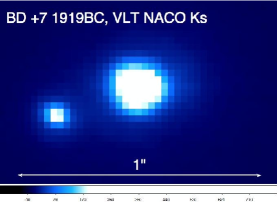
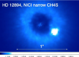
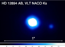
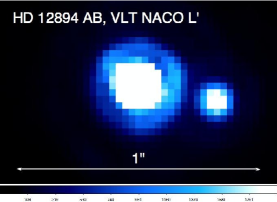
Figure 16: Gemini NICI and archival VLT NACO images of two newly discovered low-mass stellar companions, HD 12894B (0.46$\pm$ 0.08 M_⊙) and BD +07 1919C (0.20$\pm$0.03 M_⊙). North is up and East is left in all images.

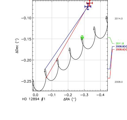
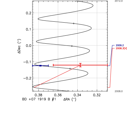
Figure 17: Sky plots for newly discovered stellar binaries, HD 12894B (left) and BD +07 1919C (right). Both new binaries share common proper motion with their parent star and HD 12894B shows clear orbital motion.

In the course of the survey, we discovered two new low mass stellar companions, HD 12894B and BD+07 1919C (Figure 16). NICI and archival datasets analyzed are tabulated in Table 10. Both companions have been confirmed to be common proper motion with their primary using VLT NACO archival data. Sky plots are shown in Figure 17 and astrometry is presented in Tables 11 and 12. Archival images were sky-subtracted and flat-fielded. Bad pixels identified from a dark image were removed. Images at different dither positions were registered and stacked. Astrometry was derived from both NICI and NACO archival datasets using the star and companion centroids measured from the final reduced stacked images.

Since the NICI datasets for these binaries either had the starspot saturated or were taken in the narrow methane filters, we calculated broadband photometry from the VLT NACO archival images. Both companions sit on the wings of the primary PSF. For these datasets, the PSF shape was generally azimuthally symmetric. To obtain photometry, we thus subtracted out a PSF radial profile generated from the azimuthal median of the star image, excluding the position angle range within $\pm$20 degrees of the detected companion. Aperture photometry was performed using 2, 3, 4, 5, and 6-pixel apertures. All apertures produced consistent results; we adopt the results using the 4-pixel aperture here. To estimate photometric errors, photometry was calculated both for individual reduced frames and the final reduced image. We adopt the rms of the values from the individual reduced frames as the photometric error. Our photometry is presented in Tables 11 and 12.

We estimate companion masses based on the models of Baraffe et al. (1998). We adopt Monte Carlo methods to account for the photometric uncertainties as well as the range of possible distances and ages for these binaries. We simulate an ensemble of 10⁶ realizations of the system, drawing from Gaussian distributions in age, parallax, and photometry with 1$\sigma$ widths taken from the measured uncertainties on these parameters. For each realization, we then interpolate with age and single-band absolute magnitude to estimate the mass of the companion from the models of Baraffe et al. (1998). The adopted mass is then the peak of the output distribution of simulated realizations, with error bars drawn from the 68% confidence limits of the output distribution. Results using J, H, and K_s single band absolute magnitudes yielded consistent results; K_s band results are presented in Tables 11 and 12. No estimate was made for the L’ band observations of HD 12894, as we could not find an apparent L’ magnitude for HD 12894 in the literature. We find best mass estimates of 0.46$\pm$ 0.08 M_⊙ for HD 12894B and 0.20$\pm$0.03 M_⊙ for BD +07 1919C.

These relatively massive (0.2–0.5 M_⊙) companions have, unsurprisingly, shown some orbital motion between the archival and NICI epochs. Thus, these orbits may yield dynamical mass measurements on a 10-20 year timescale. To determine the necessary timescales to measure these orbits, we estimate their semimajor axes and periods. Assuming a uniform eccentricity distribution between 0 $<$ e $<$ 1 and random viewing angles, Dupuy & Liu (2011) compute a median correction factor between projected separation and semimajor axis of 1.10${}^{+0.91}_{-0.36}$ (68.3% confidence limits). Using this correction factor, we derive a semimajor axis of 16.9${}^{+14.1}_{-5.6}$ AU for HD 12894AB and a semimajor axis of 13.8${}^{+11.5}_{-4.8}$ AU for BD +07 1919BC (neglecting the presence or influence of A, which lies several arcsec and $>$200 AU away). To convert from semi-major axis to period requires an estimate of the total system mass. We estimate the primary masses using the same Monte Carlo method as described above for the secondary masses, giving a mass of 1.10$\pm$0.06 M_⊙ for HD 12894 and 0.70$\pm$0.05 M_⊙ and 0.66$\pm$0.05 M_⊙ for BD+07 1919B and C respectively. Combining with the previously estimated companion masses, we estimate periods of 56${}^{+70}_{-28}$ yr for HD 12894AB and 55${}^{+69}_{-29}$ yr for BD+07 1919BC. Further orbital monitoring will thus be necessary to better constrain the semi-major axes and periods of these orbits.

4.4 PZ Tel – No debris disk

In Biller et al. (2010), we reported the detection of a 36$\pm$6 M_Jup companion to the young solar analogue PZ Tel, a member of the $\beta$ Pic moving group. Due to the considerable on-sky motion of PZ Tel B, we were able to constrain the eccentricity of the PZ Tel B orbit to $>$0.6 through Monte Carlo orbital simulations with just two epochs of NICI astrometry. Recently, this result has been confirmed by Mugrauer et al. (2012).

PZ Tel had previously been reported to have 70 $\mu$m excess emission and hence a debris disk (Rebull et al., 2008). The existence of a debris disk is hard to reconcile with the highly eccentric orbit of the brown dwarf companion, which would likely disrupt the outer debris disk as it moves through it. However, recent analysis of both Spitzer 24 and 70 $\mu$m data as well as Herschel 70, 100, and 160 $\mu$m data yield no detection of excess in any band at the location of PZ Tel AB (G. Bryden, private communication). There is a very red source $\sim$25$\arcsec$ north of PZ Tel AB which is likely extragalactic. The centroiding algorithm used by Rebull et al. (2008) allows for the centroid position to move from the target position in order to account for pointing errors and as a result likely mis-identified the extragalactic source as PZ Tel. (L. Rebull, private communication). Thus, PZ Tel does not possess a debris disk.

4.5 AB Pic B – Typical L0.5 colors with NICI

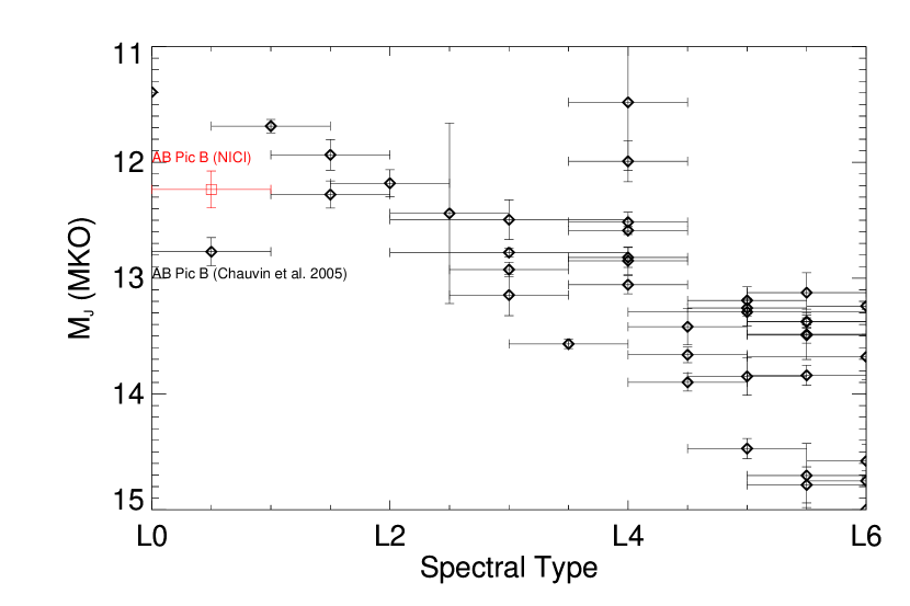
Figure 18: Infrared spectral type vs. absolute J magnitude for AB Pic B and other L0-L6 field dwarfs. Photometry for AB Pic B from Chauvin et al. (2005b) and the present study are plotted for comparison. We find a comparatively brighter J magnitude for AB Pic B compared to the photometry from Chauvin et al. (2005b), which shifts AB Pic B from being anomalously faint into the brightness sequence expected for its spectral type. Data for the comparison objects are taken from Dupuy & Liu (2012).

Chauvin et al. (2005b) reported the discovery of a faint companion to the Tuc-Hor association star AB Pic, with an estimated mass of 13-14 M_Jup. Compared to other objects of its spectral type, AB Pic B’s published $J$-band absolute magnitude is anomalously faint for its spectral type of L0.5 (Allers & Liu, 2013; Dupuy & Liu, 2012). The published colors of this object are also quite red for its spectral type. During the NICI Campaign, we acquired new $J$ and $K_{S}$ photometry for AB Pic B, presented here in Table 13. While we measure a similarly red $J-K_{S}$=1.78$\pm$0.17 mag (vs. 2.04$\pm$0.13 mag from Chauvin et al., 2005b), we find a considerably brighter $J$ magnitude of 7.97$\pm$0.14 mag for b (vs. 8.6$\pm$0.1 mag from Chauvin et al., 2005b). In Figure 18, we plot spectral type vs. $J$ magnitude for AB Pic B and a number of comparison objects. The Chauvin et al. (2005b) photometry places AB Pic B fainter than expected for its spectral type. Assuming the measured difference in photometry is not due to true variability, our brighter $J$-band magnitude places AB Pic B firmly into the expected position for its spectral type.

5 Statistical Analyses of the NICI MG Survey

Here we present limits on the frequency of wide giant extrasolar planets based on two different statistical analyses of our achieved sensitivities for the MG sample. Two of our sample stars have confirmed planetary or planet-brown dwarf boundary companions, specifically $\beta$ Pic and AB Pic. The bona fide planet around $\beta$ Pic was not detected in our first epoch Campaign data while AB Pic B was clearly detected. Including two stars with known $<$20 M_Jup companions poses issues for determining an unbiased estimate of planet frequency from our survey. Specifically, it is unclear how much we bias our estimate of planet frequency towards higher values by including a priori known companions. Thus, for the purposes of this analysis, we exclude these two stars from the sample. In Section 5.2.4, we consider the effect of adding these two stars and their companions.

5.1 Monte Carlo Constraints on Planet Fraction

Following the method of Nielsen et al. (2008) and Nielsen & Close (2010), we use Monte Carlo methods to constrain our sensitivity to planets around each target star and combine these results to place constraints on planet fraction across our entire moving group sample. First, we simulate 10000 planets with a given semimajor axis and mass, as well as randomly selected orbital parameters and eccentricity drawn from the eccentricity distribution of radial velocity planets (Nielsen & Close, 2010). The ensemble of simulated planets in mass, semimajor axis variables are then converted to equivalent contrasts and projected separations using the COND models of Baraffe et al. (2003) and the simulated orbital parameters. This simulation was repeated at masses of 0.5 - 16.9 M_Jup, in steps of 0.164 M_Jup, and at semi-major axes of 0 - 4200 AU, with step size varying as a function of distance (0.286 AU out to 20 AU, 5.333 AU from 20 - 100 AU, 7.333 AU from 100-210 AU, 10 AU from 210 - 500 AU, 20 AU from 500 - 1000 AU, 40 AU from 1000-2000 AU, and 100 AU from 2000 to 4200 AU). The converted ensemble is then compared with the attained ASDI and ADI contrast curves for the star to derive the percentage of simulated planets detected at the particular combination of semimajor axis and mass. In cases where a candidate companion was observed in only a single epoch and thus not confirmed as background or common proper motion, we cut off the contrast curve at the separation of the unconfirmed candidate companion or utilized a shallower contrast curve from an earlier epoch where the unconfirmed candidate was not detected. A number of stars near the Galactic bulge have been dropped from this analysis due to numerous unconfirmed candidate companions, specifically: CD -54 7336, CD -31 16041, HD 159911, V343 Nor, and HD 139084B. In total, 73 stars were used for this analysis. For the ASDI contrast curve comparison, the fluxes of simulated planets are modified to simulate the effect of ASDI self-subtraction using the SpeX Prism Library of ultracool dwarfs to partition flux between the on- and off-methane absorption images (see Nielsen et al. 2013 and Nielsen & Close 2010). This contrast curve comparison procedure is then repeated along a grid of semimajor axes and masses.

After calculating the detection probability grid for each star in the sample, we use these values to place constraints on the planet frequency over the entire sample as a function of semi-major axis and mass. For a given bin in {semi-major axis, mass}, the number of planets we expect to detect is given by:

$$N(a,m)=\sum_{i=1}^{N_{obs}}f_{p}(a,m)P_{i}(a,m)$$ (1)

where $P_{i}(a,m)$ is the fraction of planets with semimajor axis and mass ($a,m$) we could detect given the achieved contrast for star $i$ (i.e. the quantity calculated in our Monte Carlo simulations) and $f_{p}(a,m)$ is the fraction of stars that have such a planet to detect, hereafter referred to as “planet fraction”.

According to radial velocity studies, higher mass stars may preferentially host giant planets compared to lower mass stars (Johnson et al., 2007, 2010). To account for this variation, we introduce a mass correction to adjust the probability that a given star hosts a planet based on that star’s mass:

$$C_{1.0}(M_{*})=\frac{F_{p}(M_{*})}{F_{p}(1.0~{}M_{\odot})}$$ (2)

where $F_{p}(M_{*})$ is the relative probability of hosting giant planets as a function of mass, based on the linear fit of planet frequency as a function of mass for RV planets from Johnson et al. (2010). The mass-corrected version of Equation 1 is then:

$$N(a,m)=\sum_{i=1}^{N_{obs}}f_{p}(a,m)P_{i}(a,m)C_{1.0}(M_{*,i})$$ (3)

We normalize this correction at 1 $M_{\odot}$ since our sample is composed primarily of FGK stars. To estimate the mass of each of our sample stars, we interpolated from the models of Siess et al. (2000). First, we converted V and V-K to M_bol and T_eff using the lookup table developed for pre-main-sequence stars in Kenyon & Hartmann (1995). Then we used the Siess et al. (2000) solar metallicity tracks for 0.1 - 7 M_⊙ stars to find the stellar mass which best reproduces the observed M_bol and T_eff.

In the zero-detection case, we use Poisson statistics to set an upper limit on the planet fraction for our entire ensemble. Assuming that planet fraction at a given semi-major axis and mass is the same for all survey stars, we remove $f_{p}$ from the sum. The 95% confidence level upper limit on planet fraction, $f_{p,95\%}$ is then:

$$f_{p,95\%}(a,m)\leq\frac{3}{\sum_{i=1}^{N_{obs}}P_{i}(a,m)C_{1.0}(M_{*,i})}$$ (4)

where 3 is the Poisson expectation value to set a 95% confidence upper limit on planet fraction in the null result case.

Many of our sample stars have binary companions, which may disrupt the formation of planets in that system. To account for the effect of binary companions, we have followed the approach detailed in Nielsen et al. (2013) and define an “exclusion zone” around each of the binaries in our sample in which we do not expect planets to form and thus where we do not simulate planets. Binaries in our sample are listed in Table 14.

We also account for nonuniform position angle coverage of our observations at large angular separations. The NICI detector is square, with the focal plane mask and target star placed offset from the center. As a result, while we image 360^∘ in position angle at small separations, at larger separations ($\gtrsim$6.3$\arcsec$) our coverage declines as some position angles are off the edge of the detector. In our Monte Carlo simulations we account for this effect by generating a uniform random variable between 0 and 1 for each simulated planet. If that random variable is greater than the fractional angular coverage at the projected separation of the simulated planet, then that planet is considered undetectable even if it is brighter than the contrast curve. This parameter is similar to the position angle of nodes (rotation of the orbit on the plane of the sky), which follows a uniform distribution. When multiple contrast curves are available for a single target star, this random variable is also preserved across all epochs so that the same set of simulated planets are compared to each contrast curve for the same star.

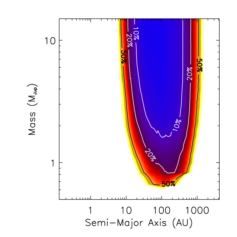
Figure 19: The 95% confidence upper limit on planet fraction as a function of semimajor axis and planet mass for our entire MG survey sample, using the models of Baraffe et al. (2002, 2003) and the Monte Carlo method described in Nielsen et al. (2008) and Nielsen & Close (2010). We also utilize here a mass correction to adjust the probability that a given star hosts a planet based on that star’s mass, drawn from the linear fit of planet frequency as a function of mass for RV planets from Johnson et al. (2010). In general, we find that giant planets are rare at wide separations in our sample: we expect less than 10$\%$ of stars to possess a 2 M_Jup planet at separations of 49 to 290 AU, at a 95$\%$ confidence level. Note that this analysis does not assume a particular distribution of planets as a function of mass and semi-major axis.

Figure 19 gives the upper limit on planet fraction $f_{p,95\%}$ as a function of semimajor axis and planet mass for our entire moving group sample, using the models of Baraffe et al. (2002) to convert between achieved survey contrast and predicted detectable planet mass. Upper limits on planet fraction as a function of semi-major axis for this analysis (i.e. single mass cuts from Figure 19) are presented in Table 15. Giant planets are rare at wide separations; for instance we expect less than 10$\%$ of stars to possess a 2 M_Jup planet at semi-major axes of 49 to 290 AU. Note that this analysis does not assume a particular distribution of planets as a function of mass and semi-major axis.

5.2 A Bayesian Analysis of the NICI MG Survey

Bayesian methods provide a powerful complement to frequentist Monte-Carlo methods for interpreting large-scale direct imaging surveys for exoplanets (see e.g.  Nielsen et al., 2008; Nielsen & Close, 2010; Bonavita et al., 2012). Frequentist Monte-Carlo methods produce useful star-by-star constraints but sometimes have difficulties interpreting positive detections. In contrast, Bayesian methods produce less useful star-by-star constraints but can seamlessly handle both null and positive detections, as well as data analysis using multiple parameter models. Here we apply the Bayesian statistical analysis method pioneered by Allen (2007) to the NICI MG sample. Our goal is to estimate the frequency of planets based on the observational constraints produced by our survey, given the limits of our sample size and sensitivity.

5.2.1 Bayes’ Theorem

Bayes’ theorem can be simply derived from the basic rules of probability and provides a powerful means to analyze and interpret data (e.g.  Sivia & Skilling, 2006). At the end of our experiment, the quantity we would like to determine is:

$$Prob(model|data,I)$$ (5)

which is the probability that a given model is correct given the data in hand as well as any other prior information $I$. This quantity is the posterior probability distribution function (henceforth posterior PDF). The power of Bayes’ theorem is it allows us to relate the posterior PDF to other, more easily calculated quantities:

$$Prob(model|data,I)\propto Prob(data|model,I)\times Prob(model|I)$$ (6)

The quantity $Prob(data|model,I)$ is known as the likelihood function – it is the probability of obtaining the data on hand given a specific model and additional prior information. The quantity $Prob(model|I)$ is known as the prior probability (or simply the prior) and includes any additional prior information we know about the problem. Thus, by formulating reasonable likelihood functions and priors for a direct imaging planet detection survey, we can derive the posterior PDF and constrain models for the underlying planet population.

5.2.2 Description of Method

Calculating the posterior PDF for one bin in observable space

We adapt the method established in Allen (2007) and Kraus et al. (2011) for studying stellar binarity in the context of a direct imaging survey of exoplanets. Allen (2007) model the distributions of substellar and stellar binary mass ratios and semi-major axis as a power law in mass ratio and a Gaussian in semi-major axis (henceforth $a$). For exoplanet companions to stars, we adopt instead the form of the power law distributions derived for RV planets by Cumming et al. (2008), and consider only the planet mass (henceforth $m$) rather than the mass ratio adopted for binaries:

$$\frac{dN}{dm}\propto m^{\alpha}$$ (7)

$$\frac{dN}{da}\propto a^{\beta}$$ (8)

Following the procedure of Nielsen et al. (2008) and Nielsen & Close (2010), we extend the semi-major axis power-law out to a limiting cutoff value, since earlier studies already rule out a significant population of giant planets at very wide separations(Nielsen & Close, 2010). While such planets do exist (e.g.  Lafrenière et al., 2008; Ireland et al., 2011), they are much less common than planets detected via radial velocity at closer separations (Fischer & Valenti, 2005; Cumming et al., 2008; Nielsen & Close, 2010).

Thus, we are left with 4 parameters to our models: the two power-law indices $\alpha$ and $\beta$, the outer cutoff of the semi-major axis distribution (henceforth $a_{max}$), and $F$, the fraction of stars with planets. We define $F$ such that the planet fraction over a given range of semimajor axes and masses is:

$$F=C_{0}\int_{m_{min}}^{m_{max}}\int_{a_{min}}^{a_{max}}\!m^{\alpha}a^{\beta}\,\mathrm{d}m~{}\mathrm{d}a$$ (9)

where C₀ is a normalization constant (and thus a function of F, $\alpha$, $\beta$, and a_max).

The probability to find a planet around a star in a given {semi-major axis, mass} bin, for a particular set of values for $\alpha$, $\beta$, $a_{max}$, and $F$, is then the planet fraction within that bin:

$$R(a,m|\alpha,\beta,a_{max},F)=F_{bin}=C_{0}(F,\alpha,\beta,a_{max})m^{\alpha}a^{\beta},~{}~{}~{}~{}~{}~{}a\leq a_{max}$$ (10)

$$R(a,m|\alpha,\beta,a_{max},F)=F_{bin}=0,~{}~{}~{}~{}~{}~{}a>a_{max}$$ (11)

where C₀ can be determined from Equation 9.

To compute the likelihood, we calculate how many planets we expect to detect with this model in each {semimajor axis, mass} bin and compare with the actual number of planets (generally 0) detected in each bin, accounting for projection effects between semi-major axis and projected separation. For a given {semimajor axis, mass} bin and set of model parameters, the number of planets predicted will be:

$$N_{pred}(a,m)=N_{obs}R(a,m|\alpha,\beta,a_{max},F)$$ (12)

where N_obs is the number of times this {semimajor axis, mass} bin was observed in our survey (derived from the contrast curves and stellar properties of each survey star). For instance, if we observe 50 stars in our survey and 30 of the observed stars have contrasts deep enough to image a 10 M_Jup planet at a semimajor axis of 10 AU, then $N_{obs}$(10 AU, 10 $M_{Jup})$ = 30. We then wish to compare $N_{pred}$ with $N_{det}$, the number of planets detected for a given {semimajor axis, mass} bin. To compare data and model, we need to adopt a likelihood estimator. Since we expect to detect only small numbers of planets, our survey can be treated as a counting experiment. Thus, we adopt Poisson statistics to calculate the likelihood:

$$likelihood=prob(N_{det}|\alpha,\beta,a_{max},F)=\frac{N_{pred}^{N_{det}}exp(-N_{det})}{N_{det}!}$$ (13)

To derive the posterior PDF for this bin, we must multiply the likelihood by any prior probability distribution for our parameters. For now, we adopt the simple uniform priors for $\alpha$, $\beta$, F, and a_max:

$$prob(\alpha|I)=prob(\beta|I)=prob(F|I)=prob(a_{max}|I)=1$$ (14)

Multiplying the likelihood and prior then yields the posterior PDF for this {semimajor axis, mass} bin.

Generalization across observable space

In the last section, we showed how to calculate the posterior PDF for one {semimajor axis, mass} bin. This can be generalized across all {semimajor axis, mass} bins for the survey fairly easily. We generalize $N_{obs}$ and $N_{det}$ into 2d arrays for each {projected separation, mass} bin observed, which we will henceforth call the window function and detection array, respectively.

To build the window function, we use the contrast curve for each survey star to define the ranges in separation and mass where planets can be detected and the ranges where the contrast is insufficient to do so. Often stars were observed in both ADI and ASDI modes; in these cases, we adopt the best contrast value from the available curves at each given separation. When ASDI contrast curves are used, they are corrected for spectral self-subtraction, assuming no methane absorption (i.e. the most conservative contrast case). In cases where a candidate companion was observed in only a single epoch and thus not confirmed as background or common proper motion, we cut off the contrast curve at the separation of the unconfirmed candidate companion or utilized a shallower contrast curve from an earlier epoch where the unconfirmed candidate was not detected. A number of stars near the Galactic bulge have been dropped from this analysis due to numerous unconfirmed candidate companions, specifically: CD -54 7336, CD -31 16041, HD 159911, V343 Nor, and HD 139084B. In total, 73 stars were used for this analysis. Bins where a planet can be detected are assigned a value of 1 and bins where no planet can be detected are assigned a value of 0. We account for nonuniform position angle coverage of our contrast curves by multiplying the window function for each star by the fractional coverage at each separation. We then convert the window function expressed in projected angular separation and contrast to projected physical separation and estimated mass using the known distance and age of each star and either the DUSTY models of Baraffe et al. (2002) or the COND models of Baraffe et al. (2003). The detection array is set up in a similar manner — as a simple array with the number of objects detected in each {separation,mass} bin. As exoplanets cool with age, dust should condense from their atmospheres, producing a transition from red, dusty spectra (DUSTY) to bluer spectra characterized by methane absorption (COND). However, no directly imaged planet to date has yet to show methane absorption in the near-IR, so we choose here to present results using both of these models.

We then calculate the posterior PDF for each {separation, mass} point. This calculation is accomplished using a small scale Monte-Carlo simulation. At each physical separation point, we simulate 10⁶ planetary orbits, drawing eccentricity, orbital phase, and other orbital elements randomly. We solve for the semi-major implied for each simulated orbit, then produce a histogram of the result with a 5 AU binsize. The posterior PDF is calculated for each semi-major axis bin in this histogram and then weighted according to the number of simulated orbits falling into that bin to produce the posterior PDF at each given {separation, mass} point. We calculate the posterior in this manner at each {separation, mass} point and then multiply the posterior PDFs across all these points to get the full posterior PDF across observable space for this set of model parameters. This process is repeated for all sets of model parameters of interest to derive the full posterior pdf as a function of the four model parameters.

5.2.3 Results with no planet detections

To determine what section of parameter space can be ruled out by our exoplanet non-detection around MG stars, we ran the Bayesian analysis with all four parameters allowed to vary. Since our contrast curves are only 95% complete, we systematically estimate a slightly low planet fraction, but this effect is likely minor. Additionally, we have adopted hot-start models here, which predict considerably brighter planets at these young ages compared to cold-start models (for instance  Spiegel & Burrows, 2012). Thus, we predict systematically more stringent upper limits on planet fractions than would be found with cold start models. For window functions and the detection function, we considered a linear grid in separation (in AU) running from 10.5 to 1015.5 AU, with points every 5 AU and a linear grid in mass (in Jupiter masses) running from 0.2 to 19.2 $M_{Jup}$, with points every 1 $M_{Jup}$, thus fully covering the mass range of possible planets as well as low mass brown dwarfs which could plausibly form via core accretion (Schneider et al., 2011). The grids for $\alpha$ and $\beta$ were centered on the values $\alpha$=-1.16 and $\beta$=-0.61, derived from radial velocity planet distributions (Cumming et al., 2008) and converted from the logarithmic units used in Cumming et al. (2008) to linear units here. We allowed $\alpha$ to run from -2.09 to -0.16 in increments of 0.066, $\beta$ to run from -1.54 to 0.39, in increments of 0.066, $F$ to run from 0.005 to 0.972 in increments of 0.033, and semi-major axis cutoff $a_{max}$ to run from 12.5 AU to 152.5 AU in increments of 5 AU. We choose to investigate this range of semi-major axis cutoff values as a value of $a_{max}<$ 10 AU is ruled out by radial velocity studies (Cumming et al., 2008; Fischer & Valenti, 2005) and a value of $a_{max}>$ 150 AU is ruled out by previous directly imaging studies (Nielsen & Close, 2010). Planet fraction $F$, and hence also the normalization constant $C_{0}$, are calculated over the range 10 – 150 AU.

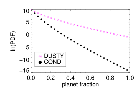
Figure 20: 1-d marginalized posterior PDFs including 4 free parameters, using the DUSTY models of Baraffe et al. (2002) (magenta asterisks) and the COND models of Baraffe et al. (2003) (black filled circles). Posterior probability is plotted in natural logarithmic units. The same plot range in ln(PDF) is used for each 1-d marginalized posterior PDF in order to clearly illustrate that, except for the planet frequency $F$, these marginalized posteriors remain unconstrained (i.e. no clear peak or trailing off to 0). Thus, we have only put confidence intervals on the planet fraction for semi-major axes between 10-150 AU. Using the DUSTY models, at a 95.4$\%$ confidence level, planet fraction must be $\leq$18$\%$ marginalized over the ranges alpha=[-2.1, -0.2], beta=[-1.5, 0.4], and cutoff=[10 AU, 150 AU]. Using the COND models, at a 95.4$\%$ confidence level, planet fraction must be $\leq$6$\%$, marginalized over the ranges alpha=[-2.1, 0.2], beta=[-1.5, 0.4], and cutoff=[10 AU, 150 AU].

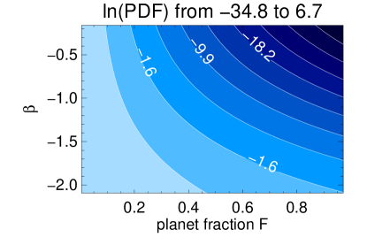
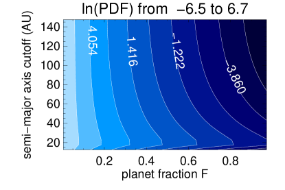
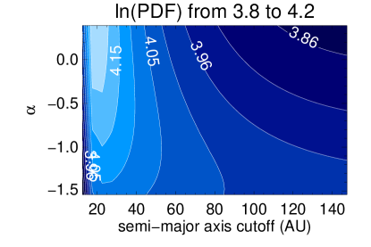
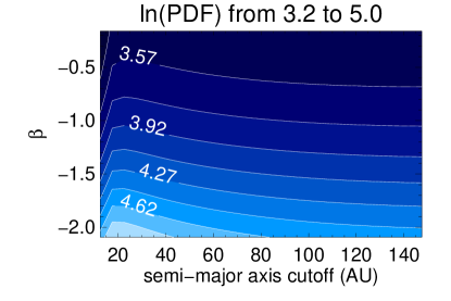
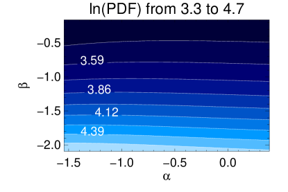
Figure 21: 2-d marginalized posterior PDFs with 4 free parameters, with contours displayed as ln(PDF) and using the DUSTY models of Baraffe et al. (2002). Posterior probability is plotted in logarithmic units, with 10 contour levels equally spaced in logarithmic space from the minimum value of each posterior PDF to the maximum value. As different posterior PDFs traverse very different probability ranges, we have included the range of ln(PDF) values plotted in the title for each subplot. Posterior PDFs which cover a greater probability range are more constrained. The ratio of these units for two different contour levels yields the relative likelihood of parameter combinations along those respective contours. Darker regions indicate parameter combinations with lower likelihood. We have not normalized these marginalized posterior PDFs, as they remain unconstrained in the null detection case.

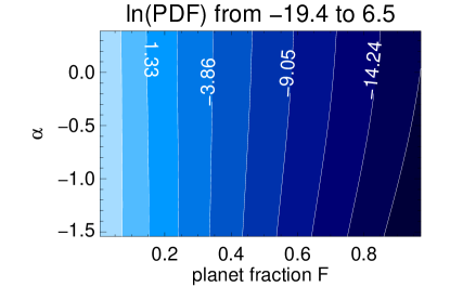
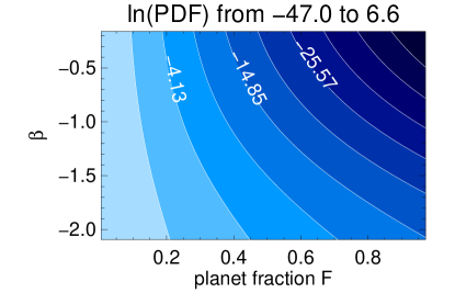
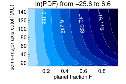
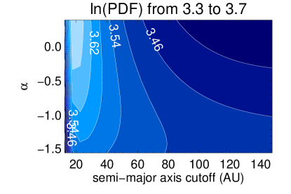
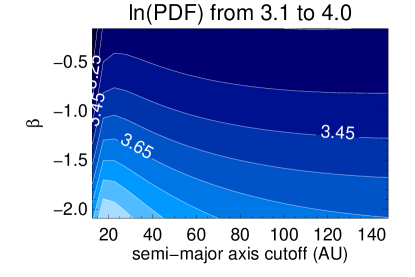
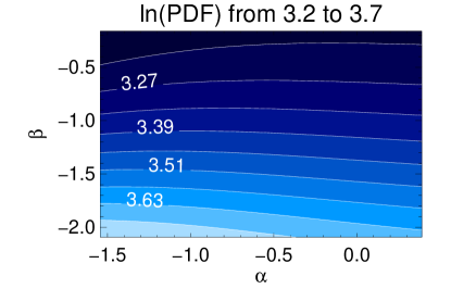
Figure 22: 2-d marginalized posterior PDFs with 4 free parameters, with contours displayed as ln(PDF) and using the COND models of Baraffe et al. (2003). Posterior probability is plotted in logarithmic units, with 10 contour levels equally spaced in logarithmic space from the minimum value of each posterior PDF to the maximum value. As different posterior PDFs traverse very different probability ranges, we have included the range of ln(PDF) values plotted in the title for each subplot. Posterior PDFs which cover a greater probability range are more constrained. The ratio of these units for two different contour levels yields the relative likelihood of parameter combinations along those respective contours. Darker regions indicate parameter combinations with lower likelihood. We have not normalized these marginalized posterior PDFs, as they remain unconstrained in the null detection case.

Obviously, the complete 4-dimensional posterior PDF cannot be fully visualized, so to present the results, we have calculated 1-d and 2-d marginalized posterior PDFs by integrating over some of the parameters. 1-d marginalized posterior PDFs are presented in Figure 20 for both DUSTY (Baraffe et al., 2002) and COND models (Baraffe et al., 2003). The 2-d marginalized posterior PDFs are presented in Figure 21 for the DUSTY models and in Figure 22 for the COND models. All PDFs are plotted in logarithmic units.

Non-detection of planets with such a large sample and deep contrasts places the strongest constraints to date on the planet fraction $F$ for directly imaged exoplanets. We derive upper limits on planet fraction $F$ by normalizing our 1-d marginalized posterior PDF for $F$. Upper limits on planet fraction $F$ are tabulated in Table 16. For the DUSTY models, a semi-major axis range of 10-150 AU, and companion masses of 1-20 M_Jup, our 95.4$\%$ confidence limit on F is $\leq$18$\%$, and at a 99.7$\%$ confidence level, $F\leq 44\%$. For the same parameter ranges and the COND models, at a 95.4$\%$ confidence level, $F\leq$6$\%$, and at a 99.7$\%$ confidence level, $F\leq$14$\%$. This is consistent with the results from our Monte Carlo simulations as well (see Table 15) and is valid for a wide range of possible planet distributions. Our results strongly constrain the frequency of planets within semi-major axes of 50 AU as well. For the DUSTY models, a semi-major axis range of 10-50 AU, and companion masses of 1-20 M_Jup, at a 95.4$\%$ confidence level, $F\leq$21$\%$, and at a 99.7$\%$ confidence level, $F\leq 51\%$. For the same parameter ranges and the COND models, at a 95.4$\%$ confidence level, $F\leq$7$\%$, and at a 99.7$\%$ confidence level, $F\leq$17$\%$. The similar constraints obtained for 10-50 AU as for 10-150 AU suggests that the 50-150 AU semi-major axis range is quite devoid of planets.

Other than for $F$, however, our marginalized posterior PDFs remain unconstrained (i.e. no clear peak or trailing off to 0) and do not cover a wide range in ln(PDF) . While the marginalized 1-d posterior PDF for planet fraction $F$ varies by over 10 orders of magnitude (Figure 20), the marginalized 1-d posteriors for the other 3 parameters vary by $<$1.5 orders of magnitude (a factor of 4.5 at most). Thus, we do not place confidence intervals on parameters other than the planet frequency $F$.

While we can place strong limits on $F$ by marginalizing over the other three parameters, determining the best-fit power law parameters for directly imaged planet populations must be deferred until there is a statistically significant population of such objects to fit. The choice of a power-law model for directly imaged planet distributions is based on fits to the properties of radial velocity planet (Cumming et al., 2008); it is not known yet whether this is the best model to describe directly imaged planet distributions.

5.2.4 Results with the AB Pic and $\beta$ Pic detections

Our Bayesian approach can seamlessly handle both planet detections and non-detections. Here we rerun the Bayesian analysis described above, this time adding in AB Pic and $\beta$ Pic, the two stars with already known planetary or low mass brown dwarf ($<$20 M_Jup) companions in our sample. We adopt a mass estimate of 8 M_Jup (i.e. the middle of the range found by  Bonnefoy et al., 2013) and a projected separation of 8.5 AU (Chauvin et al., 2012) for $\beta$ Pic b. For AB Pic B, we adopt a mass estimate of 13.5 M_Jup (Bonnefoy et al., 2010) and a projected separation of 275 AU (Chauvin et al., 2005b).

The Bayesian analysis described above was rerun with the 73 original stars, and including 1) only the $\beta$ Pic b detection, 2) only the AB Pic B detection, and 3) both detections. Results are presented in Fig. 23. Including the companions affects the shape of the marginalized PDF for planet fraction $F$ and also provide a significant constraint on $a_{max}$, the semi-major axis cutoff. The marginalized PDFs for planet fraction $F$ with $\beta$ Pic b only and for both detections now show a peak at $\sim$4$\%$, as a clear detection of a close companion rules out a zero value for planet fraction $F$ in the 10-150 AU range. For the $\beta$ Pic b only case, planet fraction $F$=0.04${}_{-0.04}^{+0.35}$, with 95.4$\%$ confidence level error bars, so, as expected, detection of a single object does not highly constrain $F$. The AB Pic B detection is at much larger separation than the $\beta$ Pic b detection, so it provides much less of a constraint on planet fraction in this range, as there is only a very slight chance that this companion has a semi-major axis $<$ 150 AU (i.e. a highly eccentric orbit). The marginalized PDF for planet fraction $F$ in this case shows some flattening at small values of $F$ but no clear peak. As in the non-detection case, $\alpha$ and $\beta$ do not cover enough range in ln(PDF) to yield useful constraints. Given that the two companions were detected in very different separation regimes, they provide contradictory constraints on cutoff, with the AB Pic B detection strongly ruling out $a_{max}$ $<$ 100 AU and the $\beta$ Pic b weakly ruling $a_{max}$ $>$ 100 AU. While it is informative to investigate how single detections with varying estimated masses and separations affect the shape of the posterior PDF, it is dangerous to draw conclusions based on such a small sample of detections. Detection of a larger cohort of similar companions is necessary to put consistent constraints on the properties of such objects

6 Discussion

While a number of giant planets and giant planet candidates have now been imaged at separations $>$20 AU, large-scale surveys illustrate that such planets are comparatively rare around main-sequence solar analogues and low mass stars. Of the ensemble of directly-imaged planets known to date, most have been discovered around A stars (HR 8799bcde, Fomalhaut b, $\beta$ Pic b, WD 0806-661; Marois et al., 2008, 2010; Kalas et al., 2008; Lagrange et al., 2009, 2010; Luhman et al., 2011; Quanz et al., 2013; Rameau et al., 2013), with a few also discovered around very young solar analogues (1RXS J160929.1$-$210524b, LkCa 15b, GSC 06214$-$00210b, Lafrenière et al., 2008; Kraus & Ireland, 2012; Ireland et al., 2011). Only one planet has been directly-imaged to date around a main-sequence solar analogue (GJ 504b; Kuzuhara et al., 2013) . Two companions right at the deuterium burning limit have recently been reported around M stars (Bowler et al., 2013; Delorme et al., 2013), but no companion with estimated mass $<$10 M_Jup has yet been imaged around a low mass star.

The small number of detected planets is not due to a lack of stars surveyed. Our NICI survey of 80 stars is the largest single sample of MG stars observed. Significant numbers of MG stars have also been observed as part of the Gemini Deep Planet survey (Lafrenière et al., 2007b), International Deep Planet Survey (Vigan et al., 2012), SDI survey (Biller et al., 2007), Deep Imaging Survey of Young, Nearby Austral Stars (Chauvin et al., 2010), A Survey of Young, Nearby, and Dusty Stars (Rameau et al., 2013a), NACO Large Program (Vigan et al. 2013), and SEEDS (Brandt et al. 2013). Based on a sample of 118 stars compiled from the surveys of Masciadri et al. (2005), Biller et al. (2007), and Lafrenière et al. (2007b), Nielsen & Close (2010) found that planets more massive than 4 M_Jup are found around $<$20$\%$ of FGKM stars in orbits between 22 and 507 AU, at 95$\%$ confidence. Chauvin et al. (2010) find a qualitatively similar result based on a sample of 88 stars (51 of which are members of young moving groups), constraining the fraction of stars with giant planets to $<$10$\%$ at semi-major axes $>$40 AU for a planet distribution extended from radial velocity power laws. With considerably higher contrasts and better inner working angles (0.3” vs. typically 0.5-0.7”), our work here directly extends these results to lower masses and smaller separations. Our results are qualitatively similar to those of Nielsen & Close (2010) but at a considerably higher confidence level. As discussed in Section 5.2.3, we confirm and extend the result of Nielsen & Close (2010): $>$5 M_Jup companions to FGKM stars are rare at separations $>$10 AU.

Johnson et al. (2007) and Johnson et al. (2010) find that for RV planets, host star mass and planet mass are related. Higher mass stars seem to preferentially host more high mass RV planets ($>$1 M_Jup) than lower mass stars, attributable to the fact that more massive stars also likely possessed more massive primordial circumstellar disks. Indeed, Johnson et al. (2007, 2010) find that $>$1 M_Jup radial velocity planets are quite rare around M stars at semi-major axes $<$5 AU. The fact that the majority of directly-imaged planets to date have been found around higher mass stars qualitatively suggests a similar conclusion may hold for the wide planet population probed by direct imaging.

We examine here whether the statistics from direct imaging surveys to date supports this assertion. The first constraints on directly imaged planet fraction for high mass AB stars have only recently been published. Janson et al. (2011) found that $<$30$\%$ of massive stars have giant planet ($>$1 M_Jup) or brown dwarf companions that formed via gravitational instability with mass $<$100 M_Jup within 300 AU at the 99$\%$ confidence level for a sample of 18 high-mass stars in the solar neighborhood, however this work does not place limits on core-accretion planets around these hosts. For a 42-star sample, Vigan et al. (2012) found that the fraction of A stars with 1 massive planet (3-14 M_Jup) from 5-300 AU was 5.9-18.8$\%$ at the 68$\%$ confidence level (assuming power law distributions for mass and semi-major axis appropriate for core-accretion planets), however the age determination for their survey stars may be overly optimistic (Nielsen et al. 2013). Our current sample is comprised of 70$\%$ stars with spectral type of K or later and contains 33 M stars, and thus can be directly compared to the samples of Vigan et al. (2012) to test whether planet fraction indeed falls with stellar mass. Using the DUSTY models, we limit the planet fraction $F$ of our sample to $\leq$3.5$\%$ at the 68$\%$ confidence level result for 1–20 M_Jup companions at semi-major axes of 10–150 AU; this is lower than the 5.9-18.8$\%$ planet fraction at a 68$\%$ confidence level found by Vigan et al. (2012). Thus, the current set of direct imaging surveys may hint that directly imaged giant planets are less common around lower mass GKM stars compared to AB stars.

7 Conclusions

As part of the Gemini NICI Planet-Finding Campaign, we imaged 80 members of nearby young moving groups, with ages from 10–200 Myr and within 100 pc. In ASDI mode, we attain median contrasts of $\Delta$(mag)=12.4, 13.9, and 14.5 mag at 0.5$\arcsec$, 1$\arcsec$, and 2$\arcsec$ respectively in the narrow band methane filters ($\lambda$=1.58 $\mu$m), with a typical standard deviation of 0.9 mag. In ADI mode, we attain median contrasts of $\Delta$(mag)=10.4, 13.2, and 15.1 mag at 0.5$\arcsec$, 1$\arcsec$, and 2$\arcsec$ respectively in $H$ band. We achieve median minimum detectable masses of 11, 5, and 3 M_Jup at 0.5$\arcsec$, 1$\arcsec$, and 2$\arcsec$ using the DUSTY models (Baraffe et al., 2002).

Candidate companions within 400 AU from the star and not in dense stellar fields that could not be confirmed or rejected as common-proper motion companions using archival data were reobserved with NICI. A total of 77 candidate companions were detected and eliminated as background contaminants. Four comoving brown dwarf or substellar companions were discovered in the moving group sample: PZ Tel B (Biller et al., 2010), CD -35 2722B (Wahhaj et al., 2011), HD 12894B (this work) and BD+07 1919C (this work). PZ Tel B and CD-35 2722B are both 30-40 M_Jup brown dwarf companions, while HD 12894B and BD+07 1919C are stellar companions with estimated masses of 0.46$\pm$0.08 M_⊙ and 0.20$\pm$0.03 M_⊙ respectively. We also retrieved the substellar companions AB Pic B (Chauvin et al., 2005b) and HR 7329 B (Lowrance et al., 2000) as well as the known stellar companion to HD 82688 (Metchev & Hillenbrand, 2009). To compare to previous published surveys, we have adopted hot start models in our statistical analysis, which predict considerably brighter planets at these young ages compared to cold start models (for instance,  Spiegel & Burrows, 2012). Thus, earlier surveys as well as our own predict systematically more stringent upper limits on planet fraction than would be found with cold start models. Nonetheless, our constraints on planet fraction are consistent with and more stringent than previous work. From a Bayesian analysis for a wide range of parameters and power-law models of planet distributions, we restrict the frequency of 1–20 M_Jup companions at semi-major axes from 10–150 AU to $<$18% at a 95.4$\%$ confidence level using DUSTY models (Baraffe et al., 2002) and to $<$6% at a 95.4$\%$ confidence level using COND models (Baraffe et al., 2003).

Table 1: Properties of MG Survey Stars

Target	RA	DEC	Distance (pc)	SpT	$V$	$H$	$Ks$	Comments
TW Hya, 10 Myr
TWA 6	10:18:28.8	-31:50:02	(77)	M0	12.00	8.18	8.04
TWA 7	10:42:30.1	-33:40:16	(28)	M2	11.06	7.12	6.90
TW Hya	11:01:52.0	-34:42:17	53.7	K6	11.34	7.56	7.30
TWA 14	11:13:26.5	-45:23:43.0	95.9	M0	$\cdots$	8.73	8.49
TWA 13A	11:21:17.2	-34:46:46	55.6	M1	11.46	7.73	7.49
TWA 13B	11:21:17.4	-34:46:50	59.7	M1	11.96	7.68	7.46
TWA 8A	11:32:41.2	-26:51:56	47.0	M3	12.23	7.66	7.43
TWA 9B	11:48:23.7	-37:28:48	46.8	M1	14.00	9.38	9.15	maybe not member
TWA 9A	11:48:24.2	-37:28:49	46.8	K5	11.32	8.03	7.85	maybe not member
TWA 25	12:15:30.8	-39:48:42.0	(51)	M1	11.62	7.50	7.31
TWA 20	12:31:38.1	-45:58:59	77.5	M3	13.00	8.69	8.41
TWA 10	12:35:04.2	-41:36:39	(52)	M2	12.96	8.48	8.19
HR 4796 B	12:36:00.56	-39:52:16	72.8	M2.5	13.3	8.53	8.35
HR 4796 A	12:36:01.2	-39:52:10	72.8	A0	5.78	5.79	5.77
Beta Pic, 12 Myr
HR 9	00:06:50.1	-23:06:27	39.4	F3	6.22	5.33	5.24
HIP 10679	02:17:24.7	+28:44:31	27.3	G2	7.83	6.36	6.26
HD 15115	02:26:16.2	+06:17:33	45.2	F4	6.83	5.86	5.82
51 Eri	04:37:36.1	-02:28:25	29.4	M1	5.24	4.77	4.54
GJ 182	04:59:34.8	+01:47:00.7	25.9	M0	10.26	6.45	6.26
HIP 23309	05:00:47.1	-57:15:25.5	26.8	M0	10.25	6.43	6.24
BD-21 1074A	05:06:49.9	-21:35:09	(18)	M1	10.60	6.39	6.12
HIP 25486	05:27:04.8	-11:54:04	27.0	F7	6.36	5.09	4.93
$\beta$ Pic	05:47:17.1	-51:03:59	19.4	A3	3.87	3.54	3.53
AO Men	06:18:28.2	-72:02:41.4	38.6	K4	10.11	6.98	6.81
HD 139084 B	15:38:56.9	-57:42:18	38.5	M5	14.80	9.45	9.19
V343 Nor	15:38:57.6	-57:42:27	38.5	K0	8.25	5.99	5.85
HD 155555 C	17:17:31.3	-66:57:05	31.4	M3	12.82	7.92	7.63
CD-54 7336	17:29:55.1	-54:15:49	(66)	K1	9.62	7.46	7.36
HD 164249B	18:03:04.1	-51:38:56	48.0	M2	12.50	8.52	8.27
HD 172555 A	18:45:26.9	-64:52:16.5	28.5	A7	4.79	4.25	4.30
TYC 9073-0762-1	18:46:52.6	-62:10:36	(54)	M1	12.31	8.05	7.85
CD-31 16041	18:50:44.5	-31:47:47	(51)	K8	11.41	7.67	7.46
PZ Tel	18:53:05.9	-50:10:50	51.5	G9	8.50	6.49	6.37
HR 7329	19:22:51.2	-54:25:24	48.2	A0	5.02	5.15	5.01
HIP 95270	19:22:58.9	-54:32:15	51.8	F6	7.09	5.98	5.91
TYC 7443-1102-1B	19:56:02.94	-32:07:18.7	(57.7)	M4	13.3	8.34	8.11
TYC 7443-1102-1A	19:56:04.37	-32:07:37.7	(57.7)	M0	11.93	8.03	7.85
HD 191089	20:09:05.2	-26:13:27	52.2	F5	7.23	6.09	6.08
GJ 799A	20:41:51.2	-32:26:06.6	10.7	M4	11.49	5.20	4.94
GJ 803	20:45:09.5	-31:20:27.1	9.9	M1	8.93	4.83	4.53
CP-72 2713	22:42:49.0	-71:42:21	(36)	K7	10.69	7.12	6.89
HIP 112312A	22:44:57.8	-33:15:01.0	23.3	M4	12.10	7.15	6.93
TX PsA	22:45:00.0	-33:15:26	(20)	M5	13.36	8.06	7.79
BD-13 6424	23:32:30.9	-12:15:52	(28)	M0	10.90	6.77	6.57
Tuc/Hor, 30 Myr
HIP 1481	00:18:26.1	-63:28:39.0	41.5	F8	7.52	6.25	6.15
HIP 2729	00:34:51.2	-61:54:58	43.9	K4	9.66	6.72	6.53
HD 12894	02:04:35.0	-54:52:54	47.8	F4	6.49	5.49	5.45
HIP 12394	02:39:35.2	-68:16:01	46.6	B9	4.09	4.43	4.25
CD-53 544	02:41:46.8	-52:59:52	(42)	K6	10.45	6.93	6.76
AF Hor	02:41:47.3	-52:59:31	(42)	M2	12.21	7.85	7.64
CD-58 553	02:42:33.0	-57:39:37	(50)	K5	11.00	7.97	7.78
HIP 24947	05:20:38.0	-39:45:18	48.3	F6	7.44	6.22	6.14
AB Pic	06:19:12.9	-58:03:15	46.1	K1	7.58	7.09	6.98
HIP 104308	21:07:51.2	-54:12:59	70.9	A5	6.72	6.12	6.07
HIP 107345	21:44:30.1	-60:58:38	43.6	M0	11.69	8.09	7.87
HIP 118121	23:57:35.0	-64:17:53	47.4	A1	5.00	4.95	4.82
AB Dor, 100 Myr
HIP 5191	01:06:26.1	-14:17:46	47.3	K1	9.54	7.43	7.34
HD 19668	03:09:42.29	-09:34:46.59	37.4	G0	8.58	6.79	6.70
HIP 17695	03:47:23.3451	-01:58:19.927	16.1	M3	11.53	7.17	6.93
HD 25457	04:02:36.7449	-00:16:08.123	18.8	F6	5.44	4.34	4.18
LP 776-25	04:52:24.4	-16:49:22	(16)	M3	11.76	7.15	6.89
GJ 2036B	04:53:30.5	-55:51:32	11.1	M3	13.92	7.24	6.89
GJ 2036A	04:53:31.2	-55:51:37	11.1	M3	11.15	6.62	6.34
HIP 25283	05:24:30.1	-38:58:10	18.0	K6	9.29	6.11	5.92
HIP 26369	05:36:55.1	-47:57:48	25.6	K6	9.87	6.83	6.61
UY Pic	05:36:56.8	-47:57:52.9	25.1	K0	8.01	5.93	5.81
BD-13 1328	06:02:21.9	-13:55:33	(39)	K4	10.71	7.89	7.77
CD-35 2722	06:09:19.2	-35:49:31	(24)	M1	11.16	7.28	7.05
HD 45270	06:22:30.9	-60:13:07.1	23.8	G1	6.59	5.16	5.05
GSC 8894-0426	06:25:56.1	-60:03:27	(22)	M3	11.7	7.47	7.21
BD+07 1919 A	08:07:09.09	+07:23:00.13	35.1	K8	10.02	7.32	7.26
HD 92945	10:43:28.3	-29:03:51.4	21.4	K1	7.81	5.77	5.66
HIP 81084	16:33:41.6081	-09:33:11.954	30.7	M0	11.40	7.78	7.55
HIP 82688	16:54:08.2	-04:20:24	46.7	G0	7.89	6.48	6.36
HD 159911	17:37:46.5	-13:14:47	(45)	K4	10.22	7.02	6.84
Her / Lyr, 200 Myr
HD 70573	08:22:49.95	+01:51:33.55	(45.7)	G1	8.74	7.28	7.19
DX Leo	09:32:43.7	+26:59:18.7	17.8	K0	7.14	5.24	5.12
GJ 560 A	14:42:30.42	-64:58:30.50	16.6	A7	3.19	2.47	2.42
HD 139664	15:41:11.38	-44:39:40.34	17.4	F5	4.68	3.73	3.80
Possible AB Dor or Her / Lyr, 200 Myr
BD +1 2447	10:28:55.5	+00:50:28	7.1	M2	9.65	5.61	5.31	likely AB Dor, Malo+2012

Table 2: NICI Campaign Observations of Moving Group Targets

Target	Date (UT)	Obs Mode	Images	Exp. Time (s)	Rotation (deg)
TW Hya, 10 Myr
TWA 6	2009-01-17	ADI	45	2718	153.0
TWA 7	2009-02-11	ASDI	45	2701	119.3
TWA 7	2009-02-11	ADI	20	1208	14.2
TWA 7	2010-02-28	ADI	20	1208	12.0
TW Hya	2009-01-18	ADI	20	1208	7.0
TW Hya	2009-01-18	ASDI	55	3302	100.7
TW Hya	2009-02-12	ADI	20	1208	7.1
TW Hya	2009-02-12	ASDI	45	2701	68.7
TWA 14	2009-01-14	ADI	45	2701	12.7
TWA 14	2010-01-10	ADI	90	2701	48.2
TWA 14	2012-03-19	ADI	45	2701	39.1
TWA 13A	2009-03-10	ADI	20	1208	3.4
TWA 13A	2009-03-10	ASDI	45	2701	13.1
TWA 13B	2009-03-11	ASDI	45	2701	26.7
TWA 8A	2009-02-08	ADI	20	1208	3.8
TWA 8A	2009-02-08	ASDI	52	3122	121.1
TWA 8A	2010-04-08	ADI	20	1208	1.0
TWA 8A	2010-04-08	ASDI	45	2701	17.2
TWA 8A	2011-04-03	ASDI	45	2701	116.7
TWA 9B	2009-03-13	ADI	45	2701	16.8
TWA 9A	2009-03-09	ADI	45	2701	28.7
TWA 9A	2010-12-26	ADI	20	1208	5.0
TWA 25	2009-03-07	ADI	20	1200	4.3
TWA 25	2009-03-07	ASDI	45	2701	14.8
TWA 25	2011-04-25	ADI	20	1200	6.2
TWA 20	2009-02-06	ADI	45	2718	21.0
TWA 20	2011-05-11	ADI	45	2718	16.2
TWA 20	2011-05-16	ASDI	45	2718	27.5
TWA 10	2009-01-15	ADI	43	2581	39.1
TWA 10	2012-04-07	ADI	20	1200	4.9
HR 4796 B	2009-02-12	ADI	45	2718	34.8
HR 4796 A	2009-01-14	ASDI	45	2821	25.2
HR 4796 A	2009-01-14	ADI	20	1208	21.8
HR 4796 A	2012-04-06	ADI	64	3793	82.4
Beta Pic, 12 Myr
HR 9	2009-12-05	ADI	20	1208	2.8
HR 9	2009-12-05	ASDI	45	2736	22.8
HIP 10679	2011-10-16	ASDI	45	2701	13.3
HD 15115	2009-12-04	ADI	20	1208	6.2
HD 15115	2009-12-04	ASDI	45	2718	17.4
HD 15115	2011-11-07	ADI	20	1185	8.6
HD 15115	2011-11-22	ADI	40	2371	13.7
51 Eri	2008-11-20	ASDI	60	3830	39.3
GJ 182	2009-02-08	ADI	20	1208	6.9
GJ 182	2009-02-08	ASDI	35	2686	18.9
HIP 23309	2009-02-07	ASDI	40	3009	26.3
HIP 23309	2009-02-07	ADI	20	1208	7.8
BD-21 1074A	2008-12-16	ASDI	45	2701	48.0
HIP 25486	2009-01-14	ASDI	45	2479	34.6
HIP 25486	2009-01-14	ADI	20	1208	12.5
Beta Pic	2008-11-22	ASDI	90	5472	68.6
Beta Pic	2009-12-03	ASDI	131	7964	66.8
Beta Pic	2009-12-04	ADI	146	8654	72.7
AO Men	2009-02-08	ADI	20	1208	7.0
AO Men	2009-02-08	ASDI	43	2581	16.2
AO Men	2010-01-10	ADI	20	1208	6.9
HD 139084 B	2009-02-11	ADI	19	1141	7.0
V343 Nor	2009-03-07	ASDI	45	2718	16.4
HD 155555 C	2009-04-08	ADI	20	1208	6.7
HD 155555 C	2009-04-08	ASDI	45	2701	16.7
HD 155555 C	2010-04-10	ADI	20	1208	5.7
CD-54 7336	2009-04-09	ASDI	45	2701	17.2
CD-54 7336	2009-04-09	ADI	20	1147	6.8
HD 164249B	2009-04-10	ASDI	36	2161	23.3
HD 164249B	2009-04-10	ADI	20	1200	10.8
HD 164249B	2010-04-09	ADI	20	1200	12.2
HD 172555 A	2009-04-09	ADI	20	1208	6.8
HD 172555 A	2009-04-09	ASDI	47	2786	22.0
TYC 9073-0762-1	2009-04-09	ADI	45	2701	20.9
TYC 9073-0762-1	2010-05-09	ADI	45	2701	14.2
CD-31 16041	2009-04-08	ADI	45	2701	14.0
PZ Tel	2009-04-11	ASDI	45	2701	16.7
PZ Tel	2009-04-11	ADI	20	1208	5.8
PZ Tel	2010-05-09	ASDI	45	2701	23.2
HR 7329	2009-04-11	ADI	20	1208	8.1
HR 7329	2009-04-11	ASDI	45	2565	22.4
HIP 95270	2009-04-13	ADI	20	1208	7.9
HIP 95270	2009-04-13	ASDI	40	2416	25.8
TYC 7443-1102-1A	2010-05-09	ADI	45	2701	9.8
TYC 7443-1102-1B	2010-05-10	ADI	45	2701	14.4
HD 191089	2010-05-11	ASDI	45	2718	24.1
HD 191089	2010-05-11	ADI	20	1208	73.1
GJ 799A	2011-05-16	ASDI	33	2006	23.2
GJ 803	2010-05-09	ASDI	59	3609	65.6
GJ 803	2010-08-28	ADI	53	3021	36.9
CP-72 2713	2011-09-13	ADI	40	2416	14.9
HIP 112312A	2010-11-22	ASDI	45	2701	8.8
HIP 112312A	2010-11-22	ADI	20	1208	2.7
TX PsA	2010-08-27	ADI	47	2821	30.0
TX PsA	2011-09-14	ADI	45	2701	76.4
BD-13 6424	2010-07-27	ADI	20	1208	15.3
BD-13 6424	2010-07-27	ASDI	44	2641	29.6
Tuc/Hor, 30 Myr
HIP 1481	2010-11-25	ASDI	45	2642	20.8
HIP 1481	2010-12-26	ADI	25	1510	14.7
HIP 2729	2011-11-22	ADI	40	2416	20.1
HD 12894	2011-11-03	ADI	40	2371	24.5
HIP 12394	2008-12-15	ASDI	42	2633	21.3
HIP 12394	2008-12-15	ADI	20	1200	7.9
CD-53 544	2011-09-15	ADI	20	1208	13.1
AF Hor	2011-11-22	ADI	32	1921	21.2
CD-58 553	2009-01-17	ADI	45	2718	18.7
HIP 24947	2008-11-22	ASDI	90	5335	32.2
AB Pic	2009-03-07	ADI	20	1208	8.9
AB Pic	2009-03-07	ASDI	45	2701	23.0
HIP 104308	2011-10-30	ADI	40	2416	17.6
HIP 107345	2011-11-03	ADI	33	1981	14.9
HIP 118121	2010-08-29	ADI	20	1208	8.5
AB Dor, 100 Myr
HIP 5191	2011-11-04	ADI	43	2598	44.0
HD 19668	2010-08-29	ADI	20	1208	9.1
HD 19668	2010-08-29	ASDI	45	2701	30.6
HIP 17695	2009-01-18	ASDI	45	2701	24.0
HIP 17695	2009-01-18	ADI	20	1208	8.4
HD 25457	2009-01-13	ASDI	45	2633	23.9
HD 25457	2009-01-13	ADI	20	1208	8.5
LP 776-25	2008-11-17	ADI	45	2687	51.3
LP 776-25	2008-11-17	ASDI	45	2687	28.3
GJ 2036B	2009-01-16	ASDI	45	2701	16.9
GJ 2036A	2008-12-16	ASDI	43	2581	26.3
GJ 2036A	2008-12-16	ADI	20	1200	11.9
HIP 25283	2009-10-30	ADI	20	1208	10.0
HIP 25283	2009-10-30	ASDI	45	2719	53.7
HIP 25283	2010-12-26	ADI	20	1208	5.3
HIP 25283	2011-10-21	ADI	20	1208	5.8
HIP 26369	2008-11-21	ASDI	47	2839	20.6
UY Pic	2009-03-13	ASDI	45	2719	24.3
UY Pic	2009-03-13	ADI	20	1208	7.4
UY Pic	2009-12-04	ADI	20	1208	10.8
UY Pic	2009-12-04	ASDI	45	2719	34.4
UY Pic	2010-04-09	ASDI	50	3021	15.1
BD-13 1328	2009-01-15	ADI	32	1933	29.2
BD-13 1328	2010-01-05	ADI	45	2718	2.8
CD-35 2722	2009-01-16	ASDI	45	2701	56.2
CD-35 2722	2009-01-16	ADI	20	1208	46.5
CD-35 2722	2010-01-10	ASDI	45	2701	49.2
HD 45270	2009-02-12	ASDI	45	2650	22.8
HD 45270	2009-02-12	ADI	20	1208	9.8
GSC 8894-0426	2008-12-17	ADI	50	3002	18.7
GSC 8894-0426	2010-02-28	ADI	50	3002	20.5
BD+07 1919 A	2009-03-12	ASDI	45	2701	18.4
BD+07 1919 A	2009-03-12	ADI	20	1208	7.7
BD+07 1919 A	2010-02-28	ADI	23	1389	11.0
HD 92945	2009-01-15	ASDI	45	2770	51.3
HD 92945	2009-01-15	ADI	20	1208	30.2
HD 92945	2010-04-08	ADI	45	2718	153.1
HD 92945	2010-04-10	ASDI	45	2770	155.6
HD 92945	2011-04-02	ADI	48	2900	9.9
HD 92945	2011-05-15	ADI	20	1208	1.1
HIP 81084	2009-04-10	ASDI	45	2701	14.8
HIP 81084	2009-04-10	ADI	27	1631	4.8
HIP 82688	2010-04-09	ADI	20	1208	9.1
HIP 82688	2010-04-09	ASDI	45	2701	25.2
HIP 82688	2011-03-21	ADI	26	1570	10.9
HD 159911	2010-04-10	ASDI	45	2701	32.7
Her / Lyr, 200 Myr
HD 70573	2009-02-07	ASDI	37	2225	20.1
HD 70573	2009-02-07	ADI	20	1208	9.3
DX Leo	2009-03-13	ASDI	45	2736	13.7
DX Leo	2009-03-13	ADI	20	1208	5.5
GJ 560 A	2009-03-11	ASDI	43	2451	19.1
HD 139664	2009-02-06	ASDI	37	2320	15.1
HD 139664	2010-05-09	ASDI	45	2821	22.7
HD 139664	2010-05-09	ADI	20	1208	14.3
Possible AB Dor or Her / Lyr, 200 Myr
BD +1 2447	2009-02-07	ADI	20	1208	7.6
BD +1 2447	2009-02-07	ASDI	45	2359	18.9

Table 3: 95% completeness $CH_{4}$-band ASDI contrasts ($\Delta$mag)

Target	0.36′′	0.5′′	0.75′′	1′′	1.5′′	2′′	3′′	4′′	5′′	7′′	Cov.	9′′	Cov.	12′′	Cov.	14.8′′	Cov.
All Stars
Median Contrast	11.0	12.4	13.4	13.9	14.3	14.5	14.6	14.5	14.4	-	-	-	-	-	-	-	-
TW Hya, 10 Myr
TWA 7	11.1	12.2	13.2	13.6	14.1	14.3	14.3	14.4	14.4	14.3	1.00	13.8	1.00	12.9	0.73	12.6	0.27
TW Hya	10.5	11.6	12.5	12.8	13.4	13.5	13.7	13.7	13.7	13.2	1.00	11.8	1.00	10.6	0.69	11.9	0.20
TWA 13A	10.7	12.1	12.7	13.0	13.4	13.4	13.3	13.4	13.1	13.1	0.95	13.1	0.65	12.7	0.32	12.1	0.07
TWA 13B	10.0	11.2	12.2	12.6	12.8	12.9	12.9	12.8	12.7	12.7	1.00	12.2	0.85	11.2	0.33	11.0	0.04
TWA 8A	11.1	12.2	13.0	13.4	13.8	13.9	14.0	14.1	14.0	14.0	1.00	13.4	1.00	12.7	0.72	12.4	0.19
TWA 25	11.3	12.6	13.5	13.8	14.0	14.2	14.0	14.0	14.0	13.8	0.97	13.4	0.72	12.2	0.27	12.6	0.04
HR 4796 A	11.6	12.6	13.6	14.0	14.8	15.0	15.0	15.1	14.8	15.0	1.00	15.0	1.00	15.0	1.00	15.0	1.00
Beta Pic, 12 Myr
HR 9	11.0	12.6	13.6	14.1	14.8	15.0	15.1	15.0	15.1	14.8	0.98	14.5	0.74	13.7	0.35	12.9	0.07
HIP 10679	11.0	12.3	13.3	13.9	14.4	14.6	14.7	14.8	14.6	14.5	0.93	14.2	0.68	13.7	0.28	13.0	0.05
HD 15115	11.4	13.0	14.1	14.5	15.0	15.1	15.2	15.0	15.0	14.9	0.98	14.6	0.71	13.8	0.29	13.1	0.04
51 Eri	9.1	10.7	12.6	13.2	13.6	13.8	13.8	13.8	13.6	13.7	0.89	13.4	0.66	12.9	0.28	12.1	0.05
GJ 182	11.4	12.9	13.8	14.2	14.8	14.9	14.9	14.9	14.7	14.7	0.98	14.2	0.74	13.1	0.30	13.5	0.05
HIP 23309	11.0	12.1	13.1	13.9	14.3	14.5	14.6	14.6	14.5	14.4	0.99	14.1	0.78	13.5	0.35	12.8	0.07
BD-21 1074A	10.6	11.7	12.6	12.8	13.2	13.9	13.9	13.8	13.8	13.3	1.00	12.8	0.89	11.9	0.52	11.9	0.07
HIP 25486	11.9	13.2	14.3	14.9	15.3	15.6	15.7	15.4	15.2	15.1	0.99	14.6	0.82	13.7	0.42	13.1	0.04
AO Men	11.0	12.4	13.2	13.8	14.3	14.2	14.3	14.2	14.2	14.1	0.98	13.7	0.73	12.8	0.28	12.8	0.05
V343 Nor	11.4	13.0	13.9	14.3	15.0	15.0	15.0	15.0	15.0	14.9	0.99	14.6	0.75	14.0	0.27	13.3	0.04
HD 155555 C	10.9	11.9	12.8	13.2	13.4	13.3	13.4	13.3	13.3	13.1	0.97	12.9	0.72	12.2	0.29	11.9	0.05
CD-54 7336	11.1	12.1	12.9	13.6	13.7	13.9	13.8	13.8	13.9	13.6	0.98	13.4	0.73	12.7	0.29	12.5	0.05
HD 164249B	10.4	11.2	11.8	12.1	12.0	12.2	11.9	12.0	11.7	11.6	1.00	11.2	0.90	10.4	0.35	10.8	0.01
HD 172555 A	11.1	12.9	14.2	14.9	15.3	15.3	15.4	15.3	15.4	15.8	1.00	17.1	1.00	19.2	1.00	21.1	1.00
PZ Tel	10.8	12.5	13.5	14.0	14.4	14.5	14.8	14.7	14.6	14.5	0.99	14.2	0.74	13.5	0.27	13.0	0.04
HR 7329	10.6	11.8	12.9	13.6	14.4	14.6	14.8	14.6	14.7	14.5	0.98	14.3	0.76	13.7	0.32	13.1	0.06
HIP 95270	12.1	13.3	14.1	14.6	14.9	14.9	15.1	15.0	14.9	14.7	0.99	14.2	0.80	12.6	0.37	12.5	0.07
HD 191089	10.6	12.1	13.4	14.0	14.5	14.7	14.7	14.7	14.8	14.5	0.95	14.3	0.75	13.9	0.33	13.0	0.07
GJ 799A	10.9	12.4	13.3	13.6	13.7	13.9	13.8	13.9	14.2	14.1	1.00	13.9	0.82	13.1	0.30	12.2	0.01
GJ 803	11.0	12.4	13.7	14.5	14.8	15.1	15.0	14.9	14.8	14.5	1.00	13.9	0.94	13.2	0.50	12.3	0.11
CP-72 2713	6.3	8.3	10.3	11.0	12.0	12.0	12.3	12.3	12.3	12.0	0.98	11.9	0.65	11.5	0.18	11.0	0.01
HIP 112312A	10.4	12.0	13.2	13.7	14.0	14.1	14.3	14.2	14.1	13.7	1.00	13.0	1.00	11.8	1.00	10.7	1.00
BD-13 6424	10.7	12.2	13.4	14.0	14.2	14.2	14.4	14.3	14.2	14.0	0.97	13.4	0.77	12.4	0.37	11.9	0.07
Tuc/Hor, 30 Myr
HIP 1481	10.7	11.9	13.2	13.6	14.0	14.2	14.1	14.1	14.0	13.9	0.99	13.4	0.74	12.4	0.31	-	-
HIP 12394	11.5	12.9	14.2	15.1	15.3	15.5	15.5	15.4	15.2	15.2	0.98	15.0	0.74	14.3	0.32	13.4	0.03
HIP 24947	11.0	12.6	13.6	14.1	14.4	14.5	14.6	14.5	14.4	14.3	0.99	13.5	0.81	12.6	0.40	12.9	0.09
AB Pic	11.7	12.8	13.8	14.1	14.4	14.6	14.4	14.4	14.2	14.2	1.00	13.7	0.74	12.7	0.35	12.2	0.06
AB Dor, 100 Myr
HIP 17695	11.5	12.7	13.6	13.8	14.3	14.4	14.3	14.3	14.2	14.1	1.00	13.4	0.78	11.4	0.32	12.0	0.06
HD 25457	11.7	13.1	14.3	15.1	15.4	15.6	15.7	15.3	15.5	15.4	0.99	14.9	0.78	14.1	0.35	14.0	0.07
LP 776-25	8.6	10.3	11.5	12.4	13.1	13.4	13.2	13.1	13.0	12.7	0.98	12.2	0.82	11.6	0.52	11.1	0.15
GJ 2036B	11.4	12.4	13.3	13.7	13.8	14.0	13.9	14.0	14.0	13.5	0.97	13.1	0.72	12.5	0.29	12.4	0.04
GJ 2036A	10.6	11.9	12.8	13.4	13.9	14.0	14.2	14.2	14.1	13.8	0.99	13.2	0.78	12.6	0.36	12.3	0.03
HIP 25283	11.6	12.9	13.9	14.6	14.9	14.6	14.6	14.6	14.5	14.2	1.00	13.4	0.91	12.7	0.54	12.1	0.10
HIP 26369	10.0	11.8	13.1	13.5	13.9	14.0	14.2	14.1	14.1	13.9	0.99	13.6	0.76	13.0	0.31	12.6	0.06
UY Pic	11.2	12.6	13.8	14.5	15.1	15.2	15.2	15.4	15.2	15.1	1.00	14.6	0.70	14.0	0.28	14.3	0.08
CD-35 2722	10.8	12.0	12.7	13.3	13.4	13.5	13.4	13.3	13.3	12.8	1.00	11.5	0.92	10.8	0.55	10.9	0.07
HD 45270	11.9	13.5	14.6	15.0	15.5	15.6	15.7	15.5	15.5	15.3	0.98	14.9	0.76	14.2	0.33	13.9	0.06
BD+07 1919 A	10.9	12.0	13.0	13.2	13.7	13.6	13.7	13.5	13.5	13.5	0.92	13.4	0.71	12.9	0.36	12.1	0.09
HD 92945	11.6	13.1	14.0	14.6	15.3	15.3	15.5	15.6	15.6	15.5	1.00	15.0	0.90	14.4	0.50	14.1	0.08
HIP 81084	11.2	12.3	13.0	13.2	13.6	13.8	13.6	13.6	13.4	13.5	1.00	13.2	0.77	12.4	0.24	12.2	0.03
HIP 82688	11.1	12.5	13.4	13.9	14.3	14.4	14.4	14.4	14.3	14.1	0.96	13.9	0.76	13.4	0.34	12.5	0.08
HD 159911	11.3	12.6	13.4	13.9	14.3	14.3	14.3	14.3	14.2	13.9	0.98	13.6	0.80	12.9	0.39	12.1	0.09
Her / Lyr, 200 Myr
HD 70573	11.2	12.4	13.1	13.6	13.9	14.1	14.1	14.1	14.2	13.8	0.99	13.3	0.75	12.4	0.30	12.2	0.05
DX Leo	10.6	12.2	13.4	14.1	14.7	14.9	14.9	15.0	15.0	14.9	1.00	14.6	0.74	13.6	0.24	12.8	0.02
GJ 560 A	10.8	12.5	13.8	14.9	15.7	15.9	15.9	15.9	15.8	15.7	0.98	15.5	0.74	14.9	0.31	14.3	0.06
HD 139664	11.6	12.9	14.5	15.2	15.8	15.7	15.7	15.8	15.6	15.6	1.00	15.3	0.78	14.7	0.33	14.2	0.03
Possible AB Dor or Her / Lyr, 200 Myr
BD +1 2447	11.6	13.0	13.9	14.3	14.8	15.3	15.3	15.2	15.1	15.0	0.98	14.8	0.74	14.2	0.30	13.7	0.05

Note. — Beyond 6.3$"$ only a fraction of each final image has data. This coverage fraction is given beside the contrast at these large separations. All the contrasts are 95% completeness contrasts, except at separations beyond 6.3$"$ where the nominal 5$\sigma$ contrast curve is used. A constant is added to the 5$\sigma$ curve so that both curves match at 6.3$"$. Median contrasts are only given for regions of 100% coverage.

Table 4: 95% completeness $H$-band ADI contrasts ($\Delta$mag)

Target	0.36′′	0.5′′	0.75′′	1′′	1.5′′	2′′	3′′	4′′	5′′	7′′	Cov.	9′′	Cov.	12′′	Cov.	14.8′′	Cov.
All Stars
Median Contrast	9.1	10.4	11.6	13.2	14.4	15.1	15.4	15.5	15.4	-	-	-	-	-	-	-	-
TW Hya, 10 Myr
TWA 6	8.9	10.0	11.4	12.5	13.6	13.9	13.8	13.6	13.5	12.7	1.00	11.2	1.00	10.5	0.73	11.0	0.38
TWA 7	7.8	9.1	10.6	12.3	14.3	15.2	15.3	15.7	15.5	15.4	0.90	15.0	0.67	13.6	0.29	13.7	0.05
TW Hya	7.4	9.3	11.7	13.0	14.4	14.9	14.9	15.0	14.9	15.1	0.88	14.7	0.63	14.0	0.26	13.4	0.04
TWA 14	9.5	11.0	12.6	13.7	14.3	14.2	14.3	14.3	14.2	14.1	0.88	13.8	0.65	13.0	0.29	11.6	0.05
TWA 13A	5.9	7.8	10.1	11.6	13.5	13.9	14.0	13.9	13.9	13.9	0.86	13.9	0.61	13.5	0.23	13.0	0.02
TWA 8A	7.1	9.0	11.2	12.9	14.4	14.7	14.9	14.7	14.6	14.7	0.87	14.7	0.60	14.4	0.21	14.5	0.02
TWA 9B	9.9	11.2	12.6	13.3	13.7	13.8	13.7	13.6	13.6	13.2	0.90	13.1	0.68	12.1	0.31	12.0	0.06
TWA 9A	9.2	10.1	11.8	12.8	14.4	14.8	14.7	14.8	14.7	14.4	0.94	14.2	0.75	13.3	0.37	13.3	0.09
TWA 25	7.6	9.6	11.6	13.2	14.5	15.0	15.0	14.9	14.9	14.9	0.87	14.7	0.62	14.4	0.24	13.6	0.03
TWA 20	9.2	10.8	12.1	13.3	14.0	14.2	14.2	14.3	14.3	14.1	0.89	13.7	0.67	12.5	0.31	11.9	0.06
TWA 10	10.2	11.2	12.8	13.8	14.7	14.7	14.5	14.5	14.2	14.0	0.95	13.4	0.80	12.8	0.27	13.0	0.03
HR 4796 B	8.6	9.9	11.4	12.4	13.5	13.5	13.5	13.4	13.1	12.5	0.94	12.1	0.78	11.8	0.39	12.0	0.11
HR 4796 A	-	10.8	12.3	13.4	15.2	15.9	16.2	16.2	16.1	17.6	0.01	21.6	0.01	27.7	0.01	33.4	0.01
Beta Pic, 12 Myr
HR 9	-	-	-	1.4	14.1	15.3	16.5	16.6	17.0	17.0	0.85	17.0	0.58	16.9	0.24	16.5	0.03
HD 15115	9.4	11.2	12.8	14.1	15.8	16.4	16.8	16.8	16.9	16.8	0.86	16.6	0.60	16.1	0.26	15.4	0.06
GJ 182	-	-	12.8	14.4	15.8	16.1	16.4	16.4	16.4	16.2	0.88	16.0	0.62	15.5	0.25	14.7	0.03
HIP 23309	-	-	11.3	12.6	14.4	15.2	15.7	15.7	15.8	15.6	0.88	15.4	0.64	14.9	0.26	14.6	0.04
HIP 25486	-	-	-	13.1	14.4	15.7	16.5	16.6	16.7	16.6	0.88	16.4	0.65	15.7	0.29	14.8	0.05
AO Men	-	5.5	11.6	13.0	14.9	15.4	15.6	15.7	15.6	15.5	0.86	15.4	0.59	15.1	0.28	14.5	0.04
HD 139084 B	6.9	8.7	10.8	11.7	12.3	12.2	12.3	12.2	12.2	12.0	0.87	12.0	0.62	11.6	0.25	10.1	0.03
HD 155555 C	6.9	8.9	10.8	12.2	13.7	14.0	14.1	14.1	14.0	14.0	0.87	13.8	0.62	13.6	0.24	13.2	0.03
CD-54 7336	8.0	9.9	12.0	13.5	14.8	15.1	15.0	15.2	15.1	15.0	0.87	14.9	0.62	14.5	0.25	14.3	0.03
HD 164249B	7.7	9.0	10.5	13.0	14.7	15.6	16.3	16.4	16.2	16.1	0.91	16.0	0.66	15.5	0.28	15.0	0.05
HD 172555 A	-	-	11.9	12.8	14.2	15.6	16.9	17.3	17.5	15.7	0.01	11.0	0.01	3.9	0.01	-	-
TYC 9073-0762-1	9.1	10.4	12.1	13.3	14.6	14.7	14.9	14.8	14.7	16.6	0.01	21.8	0.01	29.7	0.01	37.0	0.01
CD-31 16041	9.5	10.7	12.2	13.3	14.7	14.9	15.0	14.9	15.0	14.7	0.89	14.3	0.67	13.4	0.29	13.3	0.05
PZ Tel	-	-	11.8	13.2	15.0	15.5	16.1	16.0	16.1	16.0	0.87	15.8	0.62	15.5	0.25	14.9	0.03
HR 7329	-	-	-	1.4	14.4	15.5	16.6	16.7	16.8	16.9	0.88	16.7	0.63	16.0	0.26	15.7	0.04
HIP 95270	-	-	12.6	14.0	15.7	16.3	16.7	16.7	16.9	16.6	0.87	16.4	0.63	16.1	0.26	15.6	0.04
TYC 7443-1102-1B	8.6	10.1	11.5	12.8	13.6	14.0	14.0	13.9	14.1	13.8	0.90	13.5	0.66	12.1	0.29	11.8	0.05
TYC 7443-1102-1A	8.6	10.2	12.2	13.4	14.2	14.4	14.6	14.6	14.6	14.5	0.90	14.2	0.65	13.1	0.26	12.6	0.04
HD 191089	-	-	11.6	12.6	14.1	14.9	15.2	15.1	15.1	14.5	1.00	13.8	0.95	13.2	0.51	13.1	0.18
GJ 803	9.1	10.2	11.8	13.1	14.6	15.3	15.4	15.4	15.4	15.2	0.95	14.8	0.78	14.2	0.41	13.6	0.12
CP-72 2713	10.0	11.5	13.0	14.2	15.4	15.6	15.7	15.7	15.7	15.7	0.86	15.5	0.63	15.3	0.33	14.6	0.07
HIP 112312A	5.1	6.8	9.3	10.9	13.2	14.1	14.4	14.4	14.4	14.4	0.01	14.3	0.01	14.3	0.01	14.2	0.01
TX PsA	9.2	10.5	12.1	13.2	14.3	14.5	14.5	14.5	14.4	14.3	1.00	13.8	0.96	13.4	0.53	13.3	0.23
BD-13 6424	9.7	10.6	12.0	13.3	14.6	15.4	15.6	15.6	15.6	15.3	0.91	15.0	0.67	14.5	0.29	14.1	0.06
Tuc/Hor, 30 Myr
HIP 1481	-	-	11.5	12.8	14.4	15.2	15.5	15.6	15.4	15.4	0.89	15.0	0.65	13.6	0.31	13.6	0.06
HIP 2729	9.4	10.0	11.7	12.7	14.3	15.1	15.5	15.3	15.3	15.5	0.88	15.1	0.66	14.4	0.34	13.8	0.08
HD 12894	-	-	11.2	12.2	14.0	14.8	15.4	15.5	15.6	15.3	0.89	14.8	0.70	14.1	0.36	13.5	0.09
HIP 12394	-	-	-	-	10.0	16.1	17.4	17.8	17.7	17.9	0.86	17.7	0.62	17.4	0.27	16.9	0.04
CD-53 544	7.7	8.9	10.3	11.4	13.1	14.0	14.4	14.4	14.4	14.3	0.86	14.0	0.62	13.7	0.32	13.4	0.06
AF Hor	6.0	7.6	10.7	11.5	13.0	13.6	13.6	13.6	13.5	13.4	0.88	12.8	0.67	11.9	0.35	11.0	0.08
CD-58 553	8.4	9.8	11.1	12.3	13.8	14.4	14.6	14.6	14.5	14.3	0.90	13.9	0.68	12.9	0.33	12.8	0.07
AB Pic	9.1	10.5	12.4	14.0	15.1	15.4	15.6	15.4	15.5	15.2	1.00	14.8	0.93	14.3	0.48	14.0	0.08
HIP 104308	-	-	12.5	14.1	15.5	16.0	16.4	16.3	16.3	16.2	0.88	15.8	0.66	14.3	0.33	14.5	0.07
HIP 107345	9.5	10.7	12.3	13.6	14.3	14.7	14.5	14.4	14.5	14.3	0.87	14.0	0.64	13.5	0.32	12.2	0.07
HIP 118121	-	-	-	12.4	14.3	15.5	16.4	16.4	16.5	16.4	0.88	16.2	0.62	15.7	0.27	14.8	0.04
AB Dor, 100 Myr
HIP 5191	9.8	10.9	12.4	13.3	14.7	15.0	15.0	14.8	14.7	14.4	0.95	13.7	0.80	13.2	0.45	13.1	0.15
HD 19668	8.1	9.9	11.5	12.8	14.4	15.1	15.1	15.1	15.1	14.9	0.89	14.7	0.63	14.0	0.27	13.2	0.04
HIP 17695	9.1	10.8	12.6	13.5	14.8	15.1	15.3	15.5	15.3	15.2	0.87	14.9	0.62	14.4	0.27	13.5	0.04
HD 25457	9.2	10.8	11.6	12.0	13.6	14.6	16.1	16.7	17.1	17.1	0.87	16.9	0.62	16.4	0.27	15.7	0.04
LP 776-25	8.8	10.5	12.0	13.2	14.3	14.7	14.6	14.6	14.4	14.1	0.98	13.6	0.82	13.0	0.52	12.5	0.15
GJ 2036A	-	-	-	12.5	14.2	15.0	15.4	15.5	15.4	15.2	0.88	14.8	0.64	14.5	0.29	14.2	0.05
HIP 25283	10.7	12.2	13.9	15.6	17.4	18.3	18.8	18.8	18.8	18.7	0.87	19.2	0.01	22.1	0.01	24.8	0.01
UY Pic	-	-	12.3	13.3	15.0	15.7	16.8	16.8	16.9	16.6	0.96	16.1	0.81	15.8	0.36	17.3	0.09
BD-13 1328	10.0	11.2	12.6	13.8	14.8	14.8	15.0	14.9	14.9	14.8	0.85	14.7	0.58	14.6	0.25	13.2	0.03
CD-35 2722	9.3	10.0	11.4	12.6	14.0	14.0	14.0	13.9	13.7	13.2	0.97	12.5	0.84	11.6	0.44	11.6	0.15
HD 45270	-	-	4.4	14.2	15.8	16.5	17.5	17.6	17.4	17.4	0.88	17.1	0.64	16.3	0.27	15.7	0.04
GSC 8894-0426	-	-	12.6	14.1	15.4	15.7	15.8	16.0	15.8	15.7	0.90	15.2	0.68	13.9	0.33	14.9	0.06
BD+07 1919 A	9.7	11.0	12.9	14.1	15.6	16.2	16.1	16.0	15.3	16.0	0.87	15.8	0.63	15.2	0.26	14.6	0.04
HD 92945	9.9	11.0	12.4	13.9	15.3	16.1	16.8	16.9	16.9	16.9	1.00	16.5	1.00	16.3	0.25	15.8	0.02
HIP 81084	6.9	8.9	11.1	12.6	14.2	14.6	14.7	14.7	14.8	14.6	0.87	14.4	0.62	14.0	0.24	13.4	0.03
HIP 82688	8.3	10.2	12.6	13.6	15.2	15.9	16.1	16.1	16.2	16.0	0.89	15.8	0.64	15.5	0.26	14.3	0.04
Her / Lyr, 200 Myr
HD 70573	9.1	10.4	12.2	13.4	14.8	15.3	15.4	15.3	15.3	15.1	0.88	14.8	0.64	14.0	0.27	13.7	0.04
DX Leo	-	-	-	12.7	14.4	15.5	16.3	16.6	16.6	16.5	0.89	16.3	0.64	15.6	0.26	14.3	0.03
HD 139664	-	-	-	-	13.8	14.9	16.4	17.2	17.4	17.2	0.91	16.8	0.67	15.4	0.30	15.4	0.05
Possible AB Dor or Her / Lyr, 200 Myr
BD +1 2447	-	-	4.2	13.7	15.1	16.0	16.8	16.9	17.0	16.7	0.87	16.4	0.63	15.8	0.26	15.4	0.04

Note. — Beyond 6.3$"$ only a fraction of each final image has data. This coverage fraction is given beside the contrast at these large separations. All the contrasts are 95% completeness contrasts, except at separations beyond 6.3$"$ where the nominal 5$\sigma$ contrast curve is used. A constant is added to the 5$\sigma$ curve so that both curves match at 6.3$"$. Median contrasts are only given for regions of 100% coverage.

Table 5: 95% completeness $H$-band limiting magnitudes

Target	0.3′′	0.5′′	0.75′′	1′′	1.5′′	2′′	3′′	4′′	5′′
All Stars
Median Limiting Magnitude	16.4	17.7	18.9	20.1	21.6	22.0	22.5	22.5	22.5
TW Hya, 10 Myr
TWA 6	17.1	18.2	19.6	20.7	21.8	22.1	22.0	21.8	21.7
TWA 7	15.5	16.9	18.3	20.1	22.0	22.9	23.1	23.4	23.3
TW Hya	15.0	16.8	19.2	20.6	22.0	22.4	22.5	22.6	22.5
TWA 14	18.3	19.8	21.3	22.4	23.0	23.0	23.0	23.0	22.9
TWA 13A	13.6	15.6	17.8	19.3	21.2	21.6	21.8	21.7	21.7
TWA 8A	14.8	16.6	18.9	20.5	22.1	22.3	22.5	22.4	22.2
TWA 9B	19.3	20.5	22.0	22.7	23.1	23.2	23.1	23.0	23.0
TWA 9A	17.2	18.1	19.8	20.8	22.4	22.9	22.7	22.8	22.7
TWA 25	15.1	17.1	19.1	20.7	22.0	22.5	22.5	22.4	22.4
TWA 20	18.1	19.6	21.0	22.2	22.9	23.1	23.1	23.2	23.2
TWA 10	19.3	20.2	21.9	22.8	23.7	23.8	23.5	23.6	23.2
HR 4796 B	17.2	18.4	19.9	20.9	22.0	22.0	22.0	21.9	21.7
HR 4796 A	-	16.6	18.1	19.2	20.9	21.7	22.0	22.0	21.9
Beta Pic, 12 Myr
HR 9	-	-	-	6.7	19.4	20.6	21.8	22.0	22.3
HD 15115	15.2	17.0	18.6	19.9	21.6	22.2	22.6	22.6	22.8
GJ 182	-	-	19.2	20.8	22.2	22.6	22.9	22.8	22.9
HIP 23309	-	-	17.8	19.0	20.8	21.6	22.1	22.1	22.3
HIP 25486	-	-	-	18.2	19.5	20.8	21.6	21.7	21.8
Beta Pic	-	-	-	-	18.6	20.0	21.5	22.1	22.4
AO Men	-	12.5	18.6	20.0	21.9	22.4	22.6	22.7	22.6
HD 139084 B	16.4	18.1	20.2	21.2	21.8	21.6	21.8	21.7	21.6
HD 155555 C	14.8	16.9	18.7	20.1	21.6	21.9	22.0	22.0	21.9
CD-54 7336	15.5	17.5	19.6	21.1	22.3	22.7	22.5	22.8	22.6
HD 164249B	16.3	17.6	19.0	21.5	23.3	24.2	24.9	25.0	24.8
HD 172555 A	-	-	16.2	17.0	18.5	19.8	21.2	21.5	21.8
TYC 9073-0762-1	17.5	18.8	20.4	21.7	23.0	23.1	23.2	23.2	23.1
CD-31 16041	17.7	18.9	20.4	21.5	22.9	23.1	23.2	23.1	23.2
PZ Tel	-	-	18.3	19.6	21.5	22.0	22.5	22.5	22.6
HR 7329	-	-	-	6.6	19.6	20.6	21.7	21.9	22.0
HIP 95270	-	-	18.6	20.0	21.7	22.3	22.7	22.7	22.8
TYC 7443-1102-1B	16.9	18.5	19.9	21.1	22.0	22.3	22.4	22.3	22.4
TYC 7443-1102-1A	16.7	18.2	20.2	21.4	22.2	22.4	22.6	22.6	22.6
HD 191089	-	-	17.8	18.8	20.3	21.0	21.3	21.3	21.3
GJ 803	13.9	15.0	16.6	17.9	19.5	20.1	20.3	20.2	20.3
CP-72 2713	17.6	19.1	20.6	21.8	23.0	23.2	23.3	23.3	23.3
HIP 112312A	12.2	13.9	16.4	18.1	20.4	21.2	21.5	21.6	21.5
TX PsA	17.2	18.5	20.2	21.3	22.3	22.6	22.5	22.6	22.5
BD-13 6424	16.7	17.7	19.0	20.4	21.7	22.5	22.7	22.6	22.6
Tuc/Hor, 30 Myr
HIP 1481	-	-	17.8	19.1	20.6	21.4	21.7	21.8	21.6
HIP 2729	16.1	16.7	18.4	19.5	21.1	21.8	22.2	22.0	22.1
HD 12894	-	-	16.7	17.7	19.5	20.3	20.9	21.0	21.1
HIP 12394	-	-	-	-	14.5	20.6	21.8	22.2	22.2
CD-53 544	15.1	16.2	17.6	18.8	20.4	21.3	21.7	21.7	21.8
AF Hor	14.3	15.9	19.0	19.8	21.3	21.9	21.9	21.9	21.8
CD-58 553	16.6	18.0	19.4	20.5	22.1	22.6	22.8	22.8	22.7
AB Pic	16.1	17.6	19.5	21.1	22.2	22.5	22.7	22.5	22.6
HIP 104308	-	-	18.7	20.2	21.6	22.1	22.5	22.4	22.4
HIP 107345	17.6	18.8	20.3	21.7	22.4	22.8	22.6	22.5	22.6
HIP 118121	-	-	-	17.4	19.3	20.5	21.3	21.4	21.5
AB Dor, 100 Myr
HIP 5191	17.2	18.3	19.8	20.7	22.2	22.4	22.4	22.3	22.1
HD 19668	14.9	16.7	18.3	19.6	21.2	21.9	21.9	21.9	21.9
HIP 17695	16.3	17.9	19.8	20.7	22.0	22.3	22.5	22.6	22.5
HD 25457	13.5	15.1	16.0	16.3	18.0	18.9	20.5	21.0	21.5
LP 776-25	16.0	17.7	19.2	20.4	21.5	21.9	21.8	21.8	21.6
GJ 2036A	-	-	-	19.3	20.9	21.7	22.1	22.3	22.1
HIP 25283	16.8	18.3	20.0	21.7	23.5	24.4	24.9	24.9	25.0
UY Pic	-	-	18.2	19.2	21.0	21.7	22.7	22.8	22.9
BD-13 1328	18.1	19.3	20.7	21.8	22.8	22.9	23.0	23.0	22.9
CD-35 2722	16.5	17.3	18.7	19.9	21.3	21.3	21.2	21.2	21.0
HD 45270	-	-	9.5	19.4	21.0	21.7	22.6	22.7	22.6
GSC 8894-0426	-	-	20.9	22.4	23.7	24.0	24.1	24.3	24.1
BD+07 1919 A	17.0	18.3	20.2	21.5	22.9	23.5	23.4	23.3	22.6
HD 92945	15.6	16.7	18.2	19.7	21.1	21.9	22.5	22.7	22.7
HIP 81084	14.6	16.6	18.9	20.4	22.0	22.4	22.5	22.5	22.6
HIP 82688	14.8	16.6	19.1	20.1	21.7	22.4	22.6	22.6	22.7
Her / Lyr, 200 Myr
HD 70573	16.4	17.7	19.5	20.6	22.1	22.6	22.6	22.5	22.6
DX Leo	-	-	-	17.9	19.6	20.7	21.5	21.8	21.8
HD 139664	-	-	-	-	17.5	18.6	20.2	20.9	21.1
Possible AB Dor or Her / Lyr, 200 Myr
BD +1 2447	-	-	9.8	19.3	20.7	21.6	22.4	22.5	22.6

Table 6: 95% completeness minimum detectable masses (M_Jup) in ADI mode, DUSTY models

Target	0.3′′	0.5′′	0.75′′	1′′	1.5′′	2′′	3′′	4′′	5′′
All Stars
Median Detectable Mass	12.3	11.1	6.8	6.0	4.4	3.7	3.2	3.1	3.1
TW Hya, 10 Myr
TWA 6	7.7	6.4	5.1	4.2	3.5	3.3	3.3	3.5	3.5
TWA 7	6.9	5.5	4.3	3.1	1.9	1.4	1.3	1.1	1.2
TW Hya	10.9	7.1	4.7	3.7	2.8	2.6	2.5	2.4	2.5
TWA 14	6.8	5.3	4.0	3.4	3.0	3.0	3.0	3.0	3.0
TWA 13A	15.3	9.8	6.0	4.7	3.3	3.1	3.0	3.1	3.1
TWA 8A	10.7	6.9	4.8	3.6	2.6	2.4	2.3	2.4	2.5
TWA 9B	4.4	3.6	2.6	2.2	1.9	1.9	1.9	2.0	2.0
TWA 9A	6.3	5.4	4.0	3.4	2.4	2.1	2.2	2.1	2.2
TWA 25	10.4	6.6	4.7	3.6	2.8	2.4	2.4	2.5	2.5
TWA 20	6.5	5.1	4.0	3.2	2.8	2.6	2.6	2.6	2.6
TWA 10	4.6	3.9	2.9	2.2	1.7	1.7	1.8	1.8	2.0
HR 4796 B	7.4	6.0	4.7	3.9	3.3	3.2	3.2	3.3	3.5
HR 4796 A	-	8.6	6.4	5.2	3.9	3.5	3.3	3.3	3.3
Beta Pic, 12 Myr
HR 9	-	-	-	56.2	4.6	3.7	2.9	2.8	2.5
HD 15115	10.4	7.1	5.5	4.4	3.3	2.8	2.5	2.5	2.4
GJ 182	-	-	4.0	2.9	2.0	1.7	1.5	1.5	1.5
HIP 23309	-	-	5.3	4.2	3.0	2.4	2.1	2.0	2.0
HIP 25486	-	-	-	4.9	3.9	3.0	2.4	2.4	2.3
Beta Pic	-	-	-	-	4.0	3.1	2.0	1.6	1.3
AO Men	-	19.3	5.3	4.1	2.8	2.4	2.3	2.2	2.3
HD 139084 B	7.4	5.7	4.0	3.3	2.9	2.9	2.9	2.9	3.0
HD 155555 C	9.0	6.4	4.9	3.7	2.7	2.5	2.4	2.4	2.4
CD-54 7336	11.7	7.5	5.4	4.2	3.3	3.0	3.1	3.0	3.1
HD 164249B	8.1	6.6	5.3	3.3	2.1	1.5	1.2	1.2	1.2
HD 172555 A	-	-	6.8	6.0	4.8	3.8	2.9	2.6	2.4
TYC 9073-0762-1	6.9	5.7	4.4	3.4	2.5	2.4	2.4	2.4	2.4
CD-31 16041	6.6	5.5	4.3	3.5	2.5	2.4	2.3	2.4	2.3
PZ Tel	-	-	6.0	4.9	3.5	3.1	2.8	2.8	2.7
HR 7329	-	-	-	56.2	4.9	4.0	3.2	3.1	3.1
HIP 95270	-	-	5.8	4.6	3.4	2.9	2.7	2.7	2.6
TYC 7443-1102-1B	7.8	6.1	4.9	4.0	3.3	3.1	3.1	3.1	3.1
TYC 7443-1102-1A	8.1	6.3	4.7	3.7	3.2	3.1	2.9	2.9	2.9
HD 191089	-	-	6.6	5.7	4.4	3.8	3.6	3.7	3.7
GJ 803	6.8	5.8	4.4	3.5	2.4	2.0	1.9	1.9	1.9
CP-72 2713	6.0	4.7	3.6	2.7	1.9	1.7	1.7	1.7	1.7
HIP 112312A	15.4	10.0	6.2	4.8	3.1	2.5	2.3	2.2	2.2
TX PsA	5.2	4.1	3.0	2.2	1.5	1.3	1.3	1.3	1.4
BD-13 6424	6.2	5.4	4.4	3.3	2.4	1.9	1.7	1.7	1.8
Tuc/Hor, 30 Myr
HIP 1481	-	-	8.6	7.6	5.7	4.9	4.7	4.6	4.8
HIP 2729	10.4	9.6	8.1	7.4	5.4	4.7	4.3	4.5	4.5
HD 12894	-	-	9.7	8.8	7.5	6.6	5.7	5.7	5.6
HIP 12394	-	-	-	-	17.5	5.9	4.8	4.5	4.5
CD-53 544	12.2	10.0	8.8	7.8	5.9	5.0	4.7	4.7	4.7
AF Hor	17.5	10.5	7.7	6.9	5.0	4.6	4.6	4.6	4.7
CD-58 553	10.0	8.7	7.7	6.4	4.8	4.2	4.0	4.0	4.1
AB Pic	10.4	8.9	7.5	5.5	4.5	4.1	4.0	4.2	4.1
HIP 104308	-	-	8.8	7.6	5.8	5.4	5.0	5.1	5.1
HIP 107345	8.8	7.9	6.1	4.8	4.1	3.8	4.0	4.0	4.0
HIP 118121	-	-	-	9.1	7.7	6.1	5.3	5.3	5.2
AB Dor, 100 Myr
HIP 5191	19.6	12.2	11.4	10.9	10.2	10.0	10.0	10.1	10.2
HD 19668	28.8	19.6	11.9	11.3	10.4	10.1	10.0	10.0	10.0
HIP 17695	12.0	11.2	10.2	9.7	9.1	8.9	8.8	8.7	8.8
HD 25457	27.8	20.1	12.3	12.2	11.3	10.8	10.0	9.7	9.5
LP 776-25	12.1	11.3	10.5	9.9	9.3	9.1	9.2	9.2	9.3
GJ 2036A	-	-	-	10.0	9.2	8.8	8.5	8.5	8.5
HIP 25283	11.9	11.1	10.2	9.3	8.4	7.9	7.7	7.7	7.7
UY Pic	-	-	11.5	11.0	10.1	9.7	9.2	9.2	9.1
BD-13 1328	12.1	11.4	10.8	10.1	9.6	9.6	9.5	9.5	9.6
CD-35 2722	12.3	11.9	11.2	10.6	9.9	9.8	9.9	9.9	10.0
HD 45270	-	-	-	10.9	10.0	9.7	9.2	9.1	9.2
GSC 8894-0426	-	-	10.0	9.2	8.5	8.4	8.3	8.2	8.3
BD+07 1919 A	12.5	11.8	10.9	10.2	9.5	9.2	9.2	9.2	9.6
HD 92945	19.1	12.1	11.3	10.6	9.8	9.4	9.1	9.0	9.0
HIP 81084	27.4	12.5	11.4	10.6	9.8	9.6	9.5	9.5	9.5
HIP 82688	31.2	22.5	11.7	11.2	10.4	10.0	9.9	9.9	9.9
Her / Lyr, 200 Myr
HD 70573	30.2	24.7	16.9	11.9	5.7	4.7	4.6	4.7	4.7
DX Leo	-	-	-	14.8	7.7	4.6	3.9	3.6	3.6
HD 139664	-	-	-	-	16.0	11.5	5.3	4.4	4.1
Possible AB Dor or Her / Lyr, 200 Myr
BD +1 2447	-	-	42.5	9.5	8.8	8.3	7.9	7.9	7.8

Table 7: 95% completeness minimum detectable masses (M_Jup) in ADI mode, COND models

Target	0.3′′	0.5′′	0.75′′	1′′	1.5′′	2′′	3′′	4′′	5′′
All Stars
Median Detectable Mass	10.8	6.1	3.6	2.0	1.4	1.1	1.1	1.1	1.1
TW Hya, 10 Myr
TWA 6	6.1	4.2	2.6	1.8	1.3	1.1	1.2	1.3	1.3
TWA 7	4.9	3.0	1.9	1.0	1.0	1.0	1.0	1.0	1.0
TW Hya	9.7	5.1	2.2	1.4	1.0	1.0	1.0	1.0	1.0
TWA 14	4.8	2.8	1.6	1.2	1.0	1.0	1.0	1.0	1.0
TWA 13A	15.2	8.1	3.6	2.1	1.2	1.0	1.0	1.0	1.0
TWA 8A	9.4	4.9	2.3	1.3	1.0	1.0	1.0	1.0	1.0
TWA 9B	1.9	1.3	1.0	1.0	1.0	1.0	1.0	1.0	1.0
TWA 9A	4.0	2.9	1.6	1.2	1.0	1.0	1.0	1.0	1.0
TWA 25	9.0	4.5	2.1	1.3	1.0	1.0	1.0	1.0	1.0
TWA 20	4.3	2.6	1.6	1.1	1.0	1.0	1.0	1.0	1.0
TWA 10	2.0	1.5	1.0	1.0	1.0	1.0	1.0	1.0	1.0
HR 4796 B	5.7	3.6	2.2	1.5	1.1	1.1	1.1	1.2	1.3
HR 4796 A	-	7.1	4.2	2.7	1.5	1.3	1.1	1.1	1.2
Beta Pic, 12 Myr
HR 9	-	-	-	51.9	1.9	1.2	1.1	1.1	1.1
HD 15115	8.6	4.7	2.7	1.8	1.1	1.1	1.1	1.1	1.1
GJ 182	-	-	1.5	1.1	1.1	1.1	1.1	1.1	1.1
HIP 23309	-	-	2.4	1.6	1.1	1.1	1.1	1.1	1.1
HIP 25486	-	-	-	2.1	1.4	1.1	1.1	1.1	1.1
Beta Pic	-	-	-	-	1.5	1.1	1.1	1.1	1.0
AO Men	-	19.3	2.4	1.6	1.1	1.1	1.1	1.1	1.1
HD 139084 B	5.2	2.9	1.5	1.1	1.1	1.1	1.1	1.1	1.1
HD 155555 C	7.5	3.9	2.1	1.2	1.1	1.1	1.1	1.1	1.1
CD-54 7336	10.2	5.4	2.6	1.6	1.1	1.1	1.1	1.1	1.1
HD 164249B	6.3	4.1	2.4	1.1	1.1	1.1	1.0	1.0	1.0
HD 172555 A	-	-	4.4	3.3	2.0	1.3	1.1	1.1	1.1
TYC 9073-0762-1	4.6	2.9	1.7	1.1	1.1	1.1	1.1	1.1	1.1
CD-31 16041	4.1	2.7	1.7	1.1	1.1	1.1	1.1	1.1	1.1
PZ Tel	-	-	3.3	2.1	1.1	1.1	1.1	1.1	1.1
HR 7329	-	-	-	51.9	2.1	1.5	1.1	1.1	1.1
HIP 95270	-	-	3.0	1.9	1.1	1.1	1.1	1.1	1.1
TYC 7443-1102-1B	5.8	3.4	2.1	1.5	1.1	1.1	1.1	1.1	1.1
TYC 7443-1102-1A	6.3	3.7	2.0	1.2	1.1	1.1	1.1	1.1	1.1
HD 191089	-	-	4.1	2.9	1.8	1.3	1.2	1.2	1.2
GJ 803	4.4	3.0	1.8	1.1	1.1	1.1	1.1	1.1	1.1
CP-72 2713	3.2	2.0	1.2	1.1	1.1	1.1	1.1	1.1	1.1
HIP 112312A	15.1	8.3	3.6	2.0	1.1	1.1	1.1	1.1	1.1
TX PsA	2.4	1.6	1.1	1.1	1.0	1.0	1.0	1.0	1.0
BD-13 6424	3.6	2.6	1.7	1.1	1.1	1.1	1.1	1.1	1.1
Tuc/Hor, 30 Myr
HIP 1481	-	-	5.5	3.6	2.1	1.7	1.5	1.5	1.6
HIP 2729	8.7	7.6	4.5	3.2	1.9	1.5	1.4	1.5	1.5
HD 12894	-	-	7.9	6.0	3.5	2.6	2.1	2.1	2.0
HIP 12394	-	-	-	-	13.1	2.3	1.6	1.5	1.5
CD-53 544	10.7	8.2	5.8	4.0	2.3	1.7	1.5	1.5	1.5
AF Hor	13.1	8.9	3.7	2.8	1.7	1.5	1.5	1.5	1.5
CD-58 553	8.2	5.6	3.7	2.6	1.6	1.4	1.4	1.4	1.4
AB Pic	8.7	6.2	3.3	1.9	1.5	1.4	1.4	1.4	1.4
HIP 104308	-	-	5.8	3.6	2.2	1.9	1.7	1.7	1.7
HIP 107345	6.0	4.1	2.4	1.6	1.4	1.3	1.4	1.4	1.4
HIP 118121	-	-	-	6.6	3.7	2.4	1.8	1.8	1.8
AB Dor, 100 Myr
HIP 5191	11.7	10.4	6.5	4.8	3.0	2.8	2.8	2.9	3.0
HD 19668	25.0	11.7	9.0	6.1	3.6	2.9	2.8	2.8	2.8
HIP 17695	9.5	5.7	3.0	2.2	1.6	1.5	1.4	1.4	1.4
HD 25457	23.2	11.8	10.8	10.4	6.3	4.5	2.7	2.2	2.0
LP 776-25	10.1	6.1	3.7	2.5	1.8	1.7	1.7	1.7	1.8
GJ 2036A	-	-	-	2.8	1.8	1.4	1.2	1.2	1.2
HIP 25283	9.0	5.3	3.1	1.8	1.1	1.0	1.0	1.0	1.0
UY Pic	-	-	6.9	5.0	2.9	2.2	1.8	1.7	1.7
BD-13 1328	9.8	6.7	4.4	2.9	2.1	2.0	2.0	2.0	2.0
CD-35 2722	10.8	9.0	5.9	4.0	2.5	2.4	2.5	2.5	2.7
HD 45270	-	-	-	4.7	2.7	2.1	1.7	1.7	1.8
GSC 8894-0426	-	-	2.7	1.8	1.2	1.1	1.1	1.0	1.1
BD+07 1919 A	11.2	8.8	4.7	3.0	2.0	1.7	1.7	1.8	2.0
HD 92945	11.5	10.1	6.3	3.8	2.4	1.9	1.7	1.6	1.6
HIP 81084	22.2	11.2	6.5	4.0	2.3	2.0	2.0	2.0	2.0
HIP 82688	29.6	12.3	8.2	5.9	3.5	2.8	2.6	2.6	2.5
Her / Lyr, 200 Myr
HD 70573	22.6	15.0	9.6	6.5	4.2	3.7	3.6	3.7	3.7
DX Leo	-	-	-	7.8	4.9	3.5	2.7	2.6	2.6
HD 139664	-	-	-	-	8.5	6.3	4.0	3.3	3.0
Possible AB Dor or Her / Lyr, 200 Myr
BD +1 2447	-	-	42.3	2.0	1.4	1.1	1.0	1.0	1.0

Table 8: Properties of Candidate Companions

Name	#	Sep	PA	$\Delta H$	$\Delta T$	Epochs	$\chi^{2}_{\nu}$(BG)	$\chi^{2}_{\nu}$(CPM)	dof	Comp?
		($"$)	(deg)	(mag)	(years)
HIP 2729	1	9.986	30.9	10.2	8.33	3	6.61	31.72	4	BG
HD 12894	1	0.322	242.9	3.0	3.22	3	322.08	110.70	4	CPM
CD -58 553	1	6.924	85.3	10.8	4.01	4	0.06	83.96	6	BG
HD 19668	1	5.470	151.0	9.8	9.93	8	0.49	30.57	14	BG
LP 776-25	1	2.570	87.8	7.5	3.13	2	0.16	67.91	2	BG
LP 776-25	2	6.340	264.7	12.9	3.13	2	0.17	14.56	2	BG
LP 776-25	3	7.010	270.1	12.8	3.13	2	1.28	14.48	2	BG
GJ 182	1	4.870	224.7	12.5	4.25	2	2.21	249.10	2	BG
GJ 182	2	7.210	236.9	10.5	4.25	2	3.98	150.44	2	BG
HIP 25283	1	8.162	83.7	15.0	1.98	3	1.60	8.96	4	BG
UY Pic	1	0.757	138.7	11.2	1.07	3	4.98	86.99	4	BG
BD -13 1328	1	2.057	314.3	12.2	0.98	2	0.07	33.11	2	BG
CD -35 2722	1	3.148	243.8	4.7	2.76	4	12.08	5.59	6	CPM
CD -35 2722	2	9.202	105.5	10.6	2.76	4	0.24	17.96	6	BG
CD -35 2722	3	5.289	275.4	13.3	0.98	2	0.12	3.84	2	BG
AO Men	1	1.501	353.4	13.3	0.92	2	0.26	13.60	2	BG
AO Men	2	2.790	206.3	14.4	0.92	2	0.42	15.62	2	BG
AO Men	3	4.086	307.3	13.3	0.92	2	0.25	9.31	2	BG
AO Men	4	4.600	275.3	15.4	0.92	2	7.49	34.05	2	BG
AO Men	5	5.233	230.0	14.2	0.92	2	0.63	7.95	2	BG
AO Men	6	5.552	248.5	15.2	0.92	2	0.39	7.23	2	BG
AO Men	7	5.768	335.8	14.9	0.92	2	0.17	10.24	2	BG
AO Men	8	6.722	141.9	11.5	0.92	2	0.17	7.84	2	BG
AO Men	9	8.333	151.4	13.0	0.92	2	0.87	16.91	2	BG
AO Men	10	9.763	267.7	13.9	0.92	2	1.42	3.84	2	BG
AB Pic	1	5.406	175.4	6.7						CPM
GSC 8894 -0426	1	5.232	159.8	12.5	1.20	2	0.75	106.77	2	BG
BD +07 1919 B	1	0.398	108.2	2.45	0.94	2	48.10	2.07	2	CPM
BD +07 1919 A	1	4.667	86.0	16.0	0.96	2	0.06	20.36	2	BG
BD +07 1919 A	2	7.702	151.8	13.6	0.96	2	0.05	52.51	2	BG
HD 70573	1	3.490	134.0	15.5	10.27	2	0.17	17.00	2	BG
HD 70573	2	6.890	305.5	16.6	10.27	2	0.39	23.65	2	BG
DX Leo	1	4.190	183.6	12.0	4.22	2	0.25	2186.44	2	BG
TWA 6	1	2.090	285.8	11.1	6.61	2	0.38	2.50	2	BG
TWA 7	1	3.203	121.3	8.6	1.05	2	0.14	59.09	2	BG
TWA 7	2	3.931	92.4	14.5	1.05	2	0.04	62.50	2	BG
TWA 7	3	4.948	172.8	13.6	1.05	2	0.45	21.66	2	BG
TWA 14	1	2.386	261.3	11.8	3.18	3	0.40	30.76	4	BG
HD 92945	1	8.961	234.7	10.6	3.22	4	1.39	751.35	6	BG
TWA 8A	1	10.550	37.4	7.4	10.58	2	0.01	40.63	2	BG
TWA 9A	1	7.286	123.1	12.2	1.80	2	2.14	23.36	2	BG
TWA 9A	2	8.260	92.2	10.7	1.80	2	1.47	36.68	2	BG
TWA 25	1	3.499	116.9	14.8	2.13	2	0.28	93.57	2	BG
TWA 25	2	8.615	10.0	11.5	2.13	2	0.17	23.40	2	BG
TWA 25	3	8.638	60.9	13.1	2.13	2	0.22	114.03	2	BG
TWA 25	4	8.943	344.5	10.3	2.13	2	0.31	7.96	2	BG
TWA 20	1	2.903	190.5	14.1	2.27	2	0.10	55.04	2	BG
TWA 20	2	6.694	10.0	11.1	2.27	2	1.44	25.93	2	BG
TWA 10	1	9.168	313.5	12.3	3.23	2	2.27	19.11	2	BG
HR 4796 A	1	4.472	322.7	8.6	18.07	3	0.69	57.48	4	BG
HD 139664	1	1.940	48.0	13.9	1.25	2	0.89	534.56	2	BG
HD 139664	2	4.550	303.9	15.0	1.25	2	0.40	166.53	2	BG
HD 139664	3	5.620	95.0	14.5	1.25	2	0.04	265.72	2	BG
HD 139664	4	5.640	267.8	14.5	1.25	2	3.24	236.41	2	BG
HD 139664	5	6.240	115.8	13.1	1.25	2	0.27	117.47	2	BG
HD 139664	6	6.770	2.4	14.6	1.25	2	0.04	443.94	2	BG
HIP 81084	1	6.190	238.6	12.7	3.97	2	0.69	790.36	2	BG
HIP 82688	1	3.819	56.9	12.9	8.55	5	655.97	11.84	8	CPM
HIP 82688	2	2.386	316.5	14.3	0.95	2	3.85	15.74	2	BG
HIP 82688	3	7.811	283.2	7.2	1.87	2	3.31	20.03	2	BG
HD 155555 C	1	2.668	164.3	10.9	1.01	2	1.09	48.30	2	BG
HD 155555 C	2	4.735	336.3	12.8	1.01	2	0.05	52.36	2	BG
HD 155555 C	3	5.634	37.3	8.0	1.01	2	0.06	46.33	2	BG
HD 155555 C	4	6.371	292.4	11.9	1.01	2	0.33	18.38	2	BG
HD 155555 C	5	7.019	323.2	12.0	1.01	2	0.08	38.87	2	BG
HD 155555 C	6	8.049	105.7	9.6	1.01	2	1.10	6.61	2	BG
HD 172555 A	1	7.730	318.9	15.5	3.92	2	0.01	12.11	2	BG
TYC 9073-762-1	1	1.339	105.8	13.4	1.08	2	0.20	62.61	2	BG
TYC 9073-762-1	2	4.142	329.0	7.1	3.96	3	0.31	31.40	4	BG
TYC 9073-762-1	3	7.295	69.1	12.1	1.08	2	1.04	3.51	2	BG
PZ Tel	1	0.330	58.7	5.4	4.82	8	318.93	22.58	14	CPM
PZ Tel	2	3.870	167.6	10.0	2.99	4	1.43	118.26	6	BG
PZ Tel	3	5.302	37.6	14.8	3.03	2	0.06	10.23	2	BG
PZ Tel	4	6.244	309.0	15.9	3.03	2	0.01	5.67	2	BG
PZ Tel	5	8.446	335.2	10.2	3.03	2	0.11	2.56	2	BG
PZ Tel	6	8.912	160.9	11.9	3.03	2	1.75	3.63	2	BG
HR 7329	1	4.175	167.6	6.6	10.78	2	133.91	3.79	2	CPM
HIP 95270	1	4.920	254.6	13.1	3.95	2	0.08	5.08	2	BG
HIP 95270	2	6.040	276.6	11.8	3.95	2	0.04	4.36	2	BG
HIP 104308	1	1.681	281.9	12.4	0.75	2	0.68	27.31	2	BG
HIP 104308	2	2.895	264.0	15.5	0.75	2	0.05	14.08	2	BG
HIP 107345	1	13.393	109.5	7.1	36.24	3	0.06	5.50	4	BG
TX PsA	1	5.235	54.0	8.86	1.05	2	0.50	37.83	2	BG
TX PsA	2	7.209	283.2	12.1	1.05	2	0.13	137.66	2	BG

Note. — Summary of the candidate companions detected around each target star. For each candidate we list the separation and position angle at the reference epoch, the contrast between candidate and host star, the time baseline for our astrometric data, the number of epochs, the reduced chi-square statistic for the companion to be background (BG) or common proper motion (CPM), the number of degrees of freedom, and the final determination of each companion: background or common proper motion. Astrometry for individual epochs is in Table 9.

Table 9: Astrometry of Candidate Companions

			Measured Position					Background Position
Name	#	Epoch	Sep	$\sigma_{Sep}$	PA	$\sigma_{PA}$		Sep	$\sigma_{Sep}$	PA	$\sigma_{PA}$	Inst.	Comp?
			($"$)		(deg)			($"$)		(deg)
HIP 2729	1	2011.89	9.986	0.009	30.9	0.2		…	…	…	…	N	BG
		2003.56	10.174	0.024	35.3	0.5		9.990	0.012	35.671	0.191	V	BG
		2005.78	10.044	0.288	33.6	1.0		10.001	0.011	34.415	0.191	S	BG
HD 12894	1	2011.84	0.322	0.009	242.9	0.2		…	…	…	…	N	CPM
		2008.62	0.339	0.020	259.0	1.0		0.251	0.006	194.735	1.455	V	CPM
		2008.85	0.331	0.020	257.2	1.0		0.229	0.006	194.856	1.596	V	CPM
CD -58 553	1	2011.70	6.924	0.009	85.3	0.2		…	…	…	…	N	BG
		2007.69	7.265	0.040	85.2	1.0		7.266	0.016	85.734	0.194	V	BG
		2008.85	7.186	0.040	85.2	1.0		7.184	0.017	85.554	0.204	V	BG
		2009.04	7.176	0.009	85.7	0.2		7.184	0.023	85.643	0.192	N	BG
HD 19668	1	2010.66	5.470	0.009	151.0	0.2		…	…	…	…	N	BG
		2001.93	6.781	0.144	149.1	1.3		6.719	0.012	148.750	0.190	S	BG
		2002.97	6.662	0.288	150.3	2.6		6.574	0.011	148.894	0.186	S	BG
		2009.74	5.566	0.013	150.0	0.5		5.597	0.009	150.616	0.179	V	BG
		2010.82	5.429	0.013	150.0	0.5		5.444	0.009	150.758	0.183	V	BG
		2010.98	5.415	0.009	150.8	0.2		5.431	0.009	150.564	0.183	N	BG
		2011.70	5.320	0.009	151.4	0.2		5.320	0.009	151.189	0.188	N	BG
		2011.86	5.301	0.013	151.2	0.3		5.298	0.009	150.972	0.189	L	BG
LP 776-25	1	2008.87	2.570	0.009	87.8	0.2		…	…	…	…	N	BG
		2005.74	2.972	0.044	102.8	2.0		2.964	0.018	101.486	0.359	G	BG
LP 776-25	2	2008.87	6.340	0.009	264.7	0.2		…	…	…	…	N	BG
		2005.74	6.146	0.044	258.2	2.0		6.111	0.018	257.961	0.267	G	BG
LP 776-25	3	2008.87	7.010	0.009	270.1	0.2		…	…	…	…	N	BG
		2005.74	6.806	0.044	264.3	2.0		6.708	0.018	264.210	0.270	G	BG
GJ 182	1	2009.10	4.870	0.009	224.7	0.2		…	…	…	…	N	BG
		2004.85	5.150	0.015	220.3	0.2		5.101	0.013	220.783	0.235	G	BG
GJ 182	2	2009.10	7.210	0.009	236.9	0.2		…	…	…	…	N	BG
		2004.85	7.440	0.015	233.7	0.2		7.360	0.014	233.887	0.219	G	BG
HIP 25283	1	2009.83	8.162	0.009	83.7	0.2		…	…	…	…	N	BG
		2010.98	8.205	0.009	83.4	0.2		8.171	0.009	83.157	0.191	N	BG
		2011.80	8.104	0.009	83.3	0.2		8.082	0.009	82.880	0.193	N	BG
UY Pic	1	2009.19	0.757	0.009	138.7	0.2		…	…	…	…	N	BG
		2009.92	0.698	0.009	141.9	0.2		0.686	0.009	140.898	0.240	N	BG
		2010.27	0.767	0.009	142.7	0.2		0.748	0.009	141.158	0.236	N	BG
BD -13 1328	1	2009.04	2.057	0.009	314.3	0.2		…	…	…	…	N	BG
		2010.01	2.123	0.009	316.0	0.2		2.117	0.010	316.120	0.204	N	BG
CD -35 2722	1	2009.18	3.148	0.009	243.8	0.2		…	…	…	…	N	CPM
		2009.04	3.154	0.009	244.2	0.2		3.163	0.009	244.260	0.227	N	CPM
		2010.02	3.121	0.009	243.9	0.2		3.137	0.010	245.183	0.238	N	CPM
		2011.80	3.090	0.009	243.1	0.2		3.139	0.020	246.848	0.276	N	CPM
CD -35 2722	2	2009.18	9.202	0.009	105.5	0.2		…	…	…	…	N	BG
		2009.04	9.190	0.009	105.4	0.2		9.174	0.014	105.462	0.209	N	BG
		2010.02	9.175	0.009	105.2	0.2		9.161	0.015	105.114	0.209	N	BG
		2011.80	9.083	0.009	104.5	0.2		9.102	0.025	104.677	0.213	N	BG
CD -35 2722	3	2009.04	5.289	0.009	275.4	0.2		…	…	…	…	N	BG
		2010.02	5.299	0.009	276.2	0.2		5.293	0.009	276.035	0.201		BG
AO Men	1	2009.10	1.501	0.009	353.4	0.2		…	…	…	…	N	BG
		2010.02	1.443	0.009	352.7	0.2		1.442	0.009	353.031	0.230	N	BG
AO Men	2	2009.10	2.790	0.009	206.3	0.2		…	…	…	…	N	BG
		2010.02	2.851	0.009	205.5	0.2		2.845	0.008	205.802	0.199	N	BG
AO Men	3	2009.10	4.086	0.009	307.3	0.2		…	…	…	…	N	BG
		2010.02	4.053	0.009	306.3	0.2		4.053	0.009	306.592	0.183	N	BG
AO Men	4	2009.10	4.600	0.009	275.3	0.2		…	…	…	…	N	BG
		2010.02	4.568	0.009	273.1	0.2		4.598	0.010	274.551	0.216	N	BG
AO Men	5	2009.10	5.233	0.009	230.0	0.2		…	…	…	…	N	BG
		2010.02	5.266	0.009	229.2	0.2		5.274	0.011	229.542	0.167	N	BG
AO Men	6	2009.10	5.552	0.009	248.5	0.2		…	…	…	…	N	BG
		2010.02	5.578	0.009	247.5	0.2		5.578	0.008	247.892	0.195	N	BG
AO Men	7	2009.10	5.768	0.009	335.8	0.2		…	…	…	…	N	BG
		2010.02	5.715	0.009	335.3	0.2		5.715	0.010	335.517	0.185	N	BG
AO Men	8	2009.10	6.722	0.009	141.9	0.2		…	…	…	…	N	BG
		2010.02	6.772	0.009	142.0	0.2		6.767	0.010	142.238	0.175	N	BG
AO Men	9	2009.10	8.333	0.009	151.4	0.2		…	…	…	…	N	BG
		2010.02	8.407	0.009	151.4	0.2		8.384	0.010	151.576	0.208	N	BG
AO Men	10	2009.10	9.763	0.009	267.7	0.2		…	…	…	…	N	BG
		2010.02	9.739	0.009	267.2	0.2		9.769	0.010	267.389	0.191	N	BG
GSC 8894 -0426	1	2008.96	5.232	0.009	159.8	0.2		…	…	…	…	N	BG
		2010.16	5.415	0.009	159.0	0.2		5.387	0.024	159.417	0.243	N	BG
BD +07 1919 B	1	2009.19	0.398	0.009	108.2	0.2		…	…	…	…	N	CPM
		2008.25	0.358	0.027	109.7	1.0		0.463	0.009	123.833	0.508	V	CPM
BD +07 1919 A	1	2009.19	4.667	0.009	86.0	0.2		…	…	…	…	N	BG
		2010.16	4.672	0.009	84.2	0.2		4.672	0.010	84.332	0.197	N	BG
BD +07 1919 A	2	2009.19	7.702	0.009	151.8	0.2		…	…	…	…	N	BG
		2010.16	7.573	0.009	151.3	0.2		7.579	0.011	151.327	0.209	N	BG
HD 70573	1	2009.10	3.490	0.009	134.0	0.2		…	…	…	…	N	BG
		1998.83	3.450	0.120	145.7	2.0		3.526	0.017	146.119	0.365	H	BG
HD 70573	2	2009.10	6.890	0.009	305.5	0.2		…	…	…	…	N	BG
		1998.83	7.170	0.120	298.9	1.0		7.079	0.019	299.614	0.202	H	BG
DX Leo	1	2009.20	4.190	0.009	183.6	0.2		…	…	…	…	N	BG
		2004.98	5.270	0.015	190.3	0.2		5.286	0.010	190.411	0.162	G	BG
TWA 6	1	2009.04	2.090	0.009	285.8	0.2		…	…	…	…	N	BG
		2002.43	2.300	0.120	281.6	3.0		2.405	0.024	279.972	0.365	H	BG
TWA 7	1	2009.11	3.203	0.009	121.3	0.2		…	…	…	…	N	BG
		2010.16	3.316	0.009	119.5	0.2		3.307	0.012	119.658	0.196	N	BG
TWA 7	2	2009.11	3.931	0.009	92.4	0.2		…	…	…	…	N	BG
		2010.16	4.072	0.009	92.0	0.2		4.067	0.010	91.918	0.198	N	BG
TWA 7	3	2009.11	4.948	0.009	172.8	0.2		…	…	…	…	N	BG
		2010.16	4.953	0.009	170.9	0.2		4.939	0.009	171.173	0.197	N	BG
TWA 14	1	2009.04	2.386	0.009	261.3	0.2		…	…	…	…	N	BG
		2010.02	2.346	0.009	261.1	0.2		2.343	0.010	261.304	0.228	N	BG
		2012.21	2.253	0.009	260.8	0.2		2.237	0.016	261.245	0.304	N	BG
HD 92945	1	2009.04	8.961	0.009	234.7	0.2		…	…	…	…	N	BG
		2010.27	8.691	0.009	233.9	0.2		8.673	0.008	233.751	0.181	N	BG
		2011.25	8.512	0.009	233.2	0.2		8.476	0.008	233.217	0.185	N	BG
		2012.26	8.298	0.009	232.5	0.2		8.271	0.008	232.569	0.189	N	BG
TWA 8A	1	2009.10	10.550	0.009	37.4	0.2		…	…	…	…	N	BG
		1998.52	9.660	0.100	34.1	2.0		9.666	0.055	33.866	0.387	H	BG
TWA 9 A	1	2010.98	7.286	0.009	123.1	0.2		…	…	…	…	N	BG
		2009.18	7.203	0.009	123.7	0.2		7.240	0.009	123.653	0.205	N	BG
TWA 9 A	2	2010.98	8.260	0.009	92.2	0.2		…	…	…	…	N	BG
		2009.18	8.151	0.009	92.3	0.2		8.183	0.011	92.504	0.188	N	BG
TWA 25	1	2009.18	3.499	0.009	116.9	0.2		…	…	…	…	N	BG
		2011.31	3.640	0.009	114.6	0.2		3.636	0.013	114.907	0.219	N	BG
TWA 25	2	2009.18	8.615	0.009	10.0	0.2		…	…	…	…	N	BG
		2011.31	8.693	0.009	10.8	0.2		8.697	0.011	11.044	0.217	N	BG
TWA 25	3	2009.18	8.638	0.009	60.9	0.2		…	…	…	…	N	BG
		2011.31	8.830	0.009	61.1	0.2		8.817	0.012	61.199	0.197	N	BG
TWA 25	4	2009.18	8.943	0.009	344.5	0.2		…	…	…	…	N	BG
		2011.31	8.930	0.009	345.6	0.2		8.946	0.012	345.654	0.208	N	BG
TWA 20	1	2009.10	2.903	0.009	190.5	0.2		…	…	…	…	N	BG
		2011.36	2.840	0.009	187.9	0.2		2.850	0.015	187.921	0.329	N	BG
TWA 20	2	2009.10	6.694	0.009	10.0	0.2		…	…	…	…	N	BG
		2011.36	6.781	0.009	10.7	0.2		6.750	0.014	11.128	0.235	N	BG
TWA 10	1	2009.04	9.168	0.009	313.5	0.2		…	…	…	…	N	BG
		2012.27	9.102	0.009	314.5	0.2		9.061	0.017	315.137	0.251	N	BG
HR 4796 A	1	2009.04	4.472	0.009	322.7	0.2		…	…	…	…	N	BG
		1994.20	4.700	0.050	311.0	1.0		4.767	0.011	311.974	0.217	E	BG
		2012.27	4.422	0.009	324.9	0.2		4.423	0.011	325.341	0.232	N	BG
HD 139664	1	2009.10	1.940	0.009	48.0	0.2		…	…	…	…	N	BG
		2010.35	2.346	0.009	46.0	0.2		2.368	0.009	45.818	0.162	N	BG
HD 139664	2	2009.10	4.550	0.009	303.9	0.2		…	…	…	…	N	BG
		2010.35	4.560	0.009	309.1	0.2		4.554	0.010	309.390	0.194	N	BG
HD 139664	3	2009.10	5.620	0.009	95.0	0.2		…	…	…	…	N	BG
		2010.35	5.860	0.009	91.2	0.2		5.857	0.009	91.343	0.188	N	BG
HD 139664	4	2009.10	5.640	0.009	267.8	0.2		…	…	…	…	N	BG
		2010.35	5.426	0.009	271.7	0.2		5.381	0.009	271.448	0.198	N	BG
HD 139664	5	2009.10	6.240	0.009	115.8	0.2		…	…	…	…	N	BG
		2010.35	6.319	0.009	111.8	0.2		6.332	0.010	111.915	0.192	N	BG
HD 139664	6	2009.10	6.770	0.009	2.4	0.2		…	…	…	…	N	BG
		2010.35	7.140	0.009	4.3	0.2		7.137	0.010	4.341	0.185	N	BG
HIP 81084	1	2009.27	6.190	0.009	238.6	0.2		…	…	…	…	N	BG
		2005.30	6.840	0.015	234.6	0.2		6.190	0.009	238.600	0.189	G	BG
HIP 82688	1	2002.66	3.819	0.008	56.9	0.2		…	…	…	…	P	CPM
		2005.56	3.830	0.050	57.5	1.0		4.089	0.008	53.803	0.144	H	CPM
		2008.40	3.819	0.027	57.2	0.3		4.355	0.009	51.033	0.143	V	CPM
		2010.27	3.791	0.009	58.8	0.2		4.538	0.010	49.339	0.147	N	CPM
		2011.21	3.786	0.009	57.9	0.2		4.634	0.011	48.566	0.149	N	CPM
HIP 82688	2	2010.27	2.386	0.009	316.5	0.2		…	…	…	…	N	BG
		2011.21	2.423	0.009	317.9	0.2		2.446	0.009	318.859	0.193		BG
HIP 82688	3	2010.27	7.811	0.009	283.2	0.2		…	…	…	…	N	BG
		2008.40	7.860	0.030	279.9	0.5		7.819	0.009	281.564	0.204	V	BG
HD 155555 C	1	2009.27	2.668	0.009	164.3	0.2		…	…	…	…	N	BG
		2010.27	2.547	0.009	163.6	0.2		2.542	0.010	163.015	0.229	N	BG
HD 155555 C	2	2009.27	4.735	0.009	336.3	0.2		…	…	…	…	N	BG
		2010.27	4.859	0.009	337.2	0.2		4.853	0.009	337.196	0.212	N	BG
HD 155555 C	3	2009.27	5.634	0.009	37.3	0.2		…	…	…	…	N	BG
		2010.27	5.754	0.009	36.7	0.2		5.758	0.008	36.639	0.193	N	BG
HD 155555 C	4	2009.27	6.371	0.009	292.4	0.2		…	…	…	…	N	BG
		2010.27	6.418	0.009	293.7	0.2		6.404	0.010	293.605	0.207	N	BG
HD 155555 C	5	2009.27	7.019	0.009	323.2	0.2		…	…	…	…	N	BG
		2010.27	7.124	0.009	324.1	0.2		7.117	0.010	324.036	0.209	N	BG
HD 155555 C	6	2009.27	8.049	0.009	105.7	0.2		…	…	…	…	N	BG
		2010.27	8.013	0.009	105.0	0.2		8.034	0.009	104.667	0.192	N	BG
HD 172555 A	1	2009.27	7.730	0.009	318.9	0.2		…	…	…	…	N	BG
		2005.35	7.210	0.120	316.5	1.0		7.215	0.009	316.704	0.205	H	BG
TYC 9073-762-1	1	2010.35	1.339	0.009	105.8	0.2		…	…	…	…	N	BG
		2009.27	1.378	0.009	108.8	0.2		1.381	0.010	109.138	0.309	N	BG
TYC 9073-762-1	2	2010.35	4.142	0.009	329.0	0.2		…	…	…	…	N	BG
		2006.39	3.883	0.027	327.6	0.4		3.846	0.017	327.630	0.308	V	BG
		2009.27	4.070	0.009	328.7	0.2		4.058	0.009	328.538	0.210	N	BG
TYC 9073-762-1	3	2010.35	7.295	0.009	69.1	0.2		…	…	…	…	N	BG
		2009.27	7.308	0.009	69.8	0.2		7.279	0.011	69.763	0.240	N	BG
PZ Tel	1	2009.27	0.330	0.009	58.7	0.2		…	…	…	…	N	CPM
		2007.45	0.255	0.002	61.7	0.6		0.328	0.009	85.328	0.822	V	CPM
		2009.74	0.337	0.002	60.5	0.2		0.378	0.010	55.649	0.243	V	CPM
		2010.34	0.356	0.001	60.5	0.2		0.375	0.010	45.177	0.407	V	CPM
		2010.35	0.355	0.001	60.4	0.2		0.375	0.010	45.122	0.408	V	CPM
		2010.36	0.360	0.009	59.9	0.2		0.377	0.010	45.010	0.409	N	CPM
		2011.31	0.373	0.009	58.7	0.2		0.423	0.009	35.718	0.584	N	CPM
		2012.26	0.397	0.009	60.4	0.2		0.479	0.009	28.577	0.684	N	CPM
PZ Tel	2	2009.27	3.870	0.009	167.6	0.2		…	…	…	…	N	BG
		2010.36	3.780	0.009	168.1	0.2		3.774	0.009	167.516	0.199	N	BG
		2011.31	3.680	0.009	166.7	0.2		3.694	0.010	167.555	0.206	N	BG
		2012.26	3.609	0.009	167.1	0.2		3.615	0.010	167.570	0.215	N	BG
PZ Tel	3	2009.27	5.302	0.009	37.6	0.2		…	…	…	…	N	BG
		2006.24	5.170	0.100	39.9	0.5		5.136	0.008	39.777	0.242		BG
PZ Tel	4	2009.27	6.244	0.009	309.0	0.2		…	…	…	…	N	BG
		2006.24	6.040	0.100	307.6	0.5		6.044	0.010	307.487	0.217		BG
PZ Tel	5	2009.27	8.446	0.009	335.2	0.2		…	…	…	…	N	BG
		2006.24	8.220	0.100	335.1	0.5		8.192	0.009	334.825	0.199	A	BG
PZ Tel	6	2009.27	8.912	0.009	160.9	0.2		…	…	…	…	N	BG
		2006.24	9.100	0.100	159.9	0.5		9.171	0.009	161.149	0.212	A	BG
HR 7329	1	2009.27	4.175	0.009	167.6	0.2		…	…	…	…	N	CPM
		1998.49	4.170	0.050	166.8	0.2		5.128	0.009	166.582	0.139	H	CPM
HIP 95270	1	2009.28	4.920	0.009	254.6	0.2		…	…	…	…	N	BG
		2005.33	4.940	0.120	250.1	1.4		4.923	0.010	250.715	0.196	H	BG
HIP 95270	2	2009.28	6.040	0.009	276.6	0.2		…	…	…	…	N	BG
		2005.33	5.900	0.120	273.3	1.2		5.916	0.009	273.632	0.173	H	BG
HIP 104308	1	2011.82	1.681	0.009	281.9	0.2		…	…	…	…	N	BG
		2012.57	1.745	0.009	283.4	0.2		1.729	0.009	283.708	0.203	N	BG
HIP 104308	2	2011.82	2.895	0.009	264.0	0.2		…	…	…	…	N	BG
		2012.57	2.929	0.009	265.3	0.2		2.924	0.008	265.279	0.212	N	BG
HIP 107345	1	2011.84	13.393	0.009	109.5	0.2		…	…	…	…	N	BG
		1975.60	16.172	1.700	120.6	3.0		16.064	0.078	119.020	0.275	D	BG
		2008.61	13.606	0.144	110.5	0.5		13.592	0.013	110.533	0.221	S	BG
TX PsA	1	2010.65	5.235	0.009	54.0	0.2		…	…	…	…	N	BG
		2011.70	5.166	0.009	52.1	0.2		5.170	0.011	51.708	0.229	N	BG
TX PsA	2	2010.65	7.209	0.009	283.2	0.2		…	…	…	…	N	BG
		2011.70	7.419	0.009	283.7	0.2		7.415	0.009	283.845	0.174	N	BG

Note. — Astrometry for each candidate companion detected around our target stars from NICI and archival observations. At each epoch we give the measured separation, position angle, and uncertainties as well as the predicted separation and position angle for a background object based on the proper motion and parallax of the primary and the candidate position at the reference epoch, which is the first epoch listed for each candidate. Astrometry is taken from Gemini-South NICI (N), VLT NACO (V), Keck NIRC2 (K), VLT ISAAC (I), ESO 3.6m (E), HST NICMOS (H), HST ACS (A), Gemini-North NIRI (G), 2MASS (M), NTT SOFI (S), LBT (L), Palomar (P), and DSS (D).

Table 10: Archival Datasets for New Stellar Binaries

Target	Date (UT)	Telescope	Filter	Mode	Length (s)	Notes
BD+07 1919	2008-04-02	VLT NACO	$J$	direct imaging	450
	2008-04-02	VLT NACO	$H$	direct imaging	450
	2008-04-02	VLT NACO	$K$s	direct imaging	150
	2009-03-12	Gemini NICI	$CH_{4}$	ASDI	2701	B saturated
						except in short exps
	2009-03-12	Gemini NICI	$H$	ADI	1208	B saturated
						in all exposures
	2010-02-28	Gemini NICI	$H$	ADI	1389	B saturated
						in all exposures
HD 12894	2008-08-14	VLT NACO	$L^{\prime}$	direct imaging	1230
	2008-11-07	VLT NACO	$K$s	direct imaging	480
	2011-11-03	Gemini NICI	$H$	ADI	2372	B saturated
						except in short exps
						A under mask

Table 11: Properties of the HD 12894 AB System

	Primary	Secondary
Parallax (mas)	20.9$\pm$0.5
Age (Myr)	30$\pm$10
Proper Motion ($\mu_{\alpha}$, $\mu_{\delta}$) (mas/yr)	(75.7$\pm$0.4, $-$25.0$\pm$0.5)
Separation: 2008.62, VLT NACO	0.33$\pm$0.02$\arcsec$ (15.7$\pm$1.0 AU)
Position Angle: 2008.62, VLT NACO	258.9$\pm$1.0∘
Separation: 2008.85, VLT NACO	0.32$\pm$0.02$\arcsec$ (15.4$\pm$1.0 AU)
Position Angle: 2008.85, VLT NACO	257.5$\pm$1.0∘
Separation: 2011.84, Gemini NICI	0.323$\pm$0.009$\arcsec$ (15.4$\pm$0.5 AU)
Position Angle: 2011.84, Gemini NICI	244.1$\pm$0.2∘
$\Delta Ks$(mag)	$\cdots$	2.96$\pm$0.03
$\Delta L^{\prime}$(mag)	$\cdots$	2.30$\pm$0.07
$Ks$ (mag)	5.52$\pm$0.02	8.48$\pm$0.04
$M_{K_{s}}$ (mag)	2.12$\pm$0.05	5.08$\pm$0.06
Spectral type	F2	$\cdots$
Estimated Mass ($M_{\odot}$)	1.10$\pm$0.06	0.46$\pm$0.08
Estimated Semi-major Axis (AU)	17${}_{-6}^{+14}$
Estimated Period (yr)	56${}_{-28}^{+70}$

Table 12: Properties of the BD+07 1919 ABC System

	Primary	Secondary	Tertiary
Parallax (mas)	28.52$\pm$2.65
Age (Myr)	70$\pm$10
Proper Motion ($\mu_{\alpha}$, $\mu_{\delta}$) (mas/yr)	(1.79$\pm$3.75, $-$138.68$\pm$3.25)
BC Separation: 2008.25, VLT NACO	0.358$\pm$0.02$\arcsec$ (12.5$\pm$1.4 AU)
BC Position Angle: 2008.25, VLT NACO	109.7$\pm$1.0∘
BC Separation: 2009.19, Gemini NICI	0.398$\pm$0.009$\arcsec$ (14.0$\pm$1.3 AU)
BC Position Angle: 2009.19, Gemini NICI	108.2$\pm$0.2∘
$\Delta J$(mag)	$\cdots$	$\cdots$	2.45$\pm$0.08
$\Delta H$(mag)	$\cdots$	$\cdots$	2.45$\pm$0.03
$\Delta Ks$(mag)	$\cdots$	$\cdots$	2.32$\pm$0.06
$J$ (mag)	7.94$\pm$0.03	8.22$\pm$0.03	10.67$\pm$0.08
$H$ (mag)	7.32$\pm$0.04	7.58$\pm$0.06	10.03$\pm$0.07
$Ks$ (mag)	7.26$\pm$0.04	7.45$\pm$0.04	9.77$\pm$0.07
$M_{J}$ (mag)	5.2$\pm$0.2	5.5$\pm$0.2	8.0$\pm$0.2
$M_{H}$ (mag)	4.6$\pm$0.2	4.8$\pm$0.2	7.3$\pm$0.2
$M_{K_{s}}$ (mag)	4.5$\pm$0.2	4.7$\pm$0.2	7.0$\pm$0.2
Estimated Mass	0.70$\pm$0.05	0.66$\pm$0.05	0.20$\pm$0.03 M⊙
Estimated Semi-major Axis (BC) (AU)	14${}_{-5}^{+12}$
Estimated Period (BC) (yr)	55${}_{-29}^{+69}$

Table 13: Photometry for AB Pic AB

	Primary	Secondary
$\Delta J$(mag)	$\cdots$	7.97$\pm$0.14
$\Delta Ks$(mag)	$\cdots$	6.79$\pm$0.10
$J$ (mag)	7.58$\pm$0.03	15.55$\pm$0.14
$Ks$ (mag)	6.98$\pm$0.03	13.77$\pm$0.10
$J$ - $Ks$ (mag)	0.60$\pm$0.04	1.78$\pm$0.17
$M_{J}$ (mag)	4.26$\pm$0.07	12.23$\pm$0.16
$M_{K_{s}}$ (mag)	3.66$\pm$0.07	10.45$\pm$0.12

Table 14: Stellar and Brown Dwarf Binaries to Sample Stars

Primary Star	Projected Separation (AU)	Sp. Type or Est. Mass	Reference
BD +7 1919A	211	K5	Dommanget & Nys (2002)
BD +7 1919B	14	$\sim$0.2 M⊙	discovered in this work
HD 12894	15.5	$\sim$0.5 M⊙	discovered in this work
PZ Tel	16.4	$\sim$40 MJup	Biller et al. (2010)
CD-35 2722	67	$\sim$30 MJup	Wahhaj et al. (2011)
HR 7329	200	M7-M8	Lowrance et al. (2000); Guenther et al. (2001)
AB Pic	250	L0.5	Chauvin et al. (2005b)
TYC 7443-1102-1	1520	M0	Lépine & Simon (2009)
CD-53 544	936	K6	companion is AF Hor, Mason et al. (2013)
AF Hor	936	M2	companion is CD -53 544, Mason et al. (2013)
GJ 2036 A	129	M3	companion is GJ 2036 B, Dommanget & Nys (2002)
GJ 2036 B	129	M3	companion is GJ 2036 A, Dommanget & Nys (2002)
HIP 26369	621	K6	companion is UY Pic, Dommanget & Nys (2002)
UY Pic	621	K0	companion is HIP 26369, Dommanget & Nys (2002)
HD 45270	376	$\cdots$	Dommanget & Nys (2002)
DX Leo	1150	M4.5	Dommanget & Nys (2002)
HIP 82688	181	0.31 M⊙	Metchev & Hillenbrand (2009)
HR 4796 A	560, 2900	M2.5, —	Dommanget & Nys (2002)
HR 4796 B	560, 2900	A0, —	Dommanget & Nys (2002)
GJ 560 A	260	K5	Dommanget & Nys (2002)
TWA 8A	611	M5	Mason et al. (2013)
TWA 9A	271	M1	comp. is TWA 9A, Dommanget & Nys (2002)
TWA 9B	271	K5	comp. is TWA 9B, Dommanget & Nys (2002)
HIP 10679	375	F5	Dommanget & Nys (2002)
BD-21 1074A	398	M3	Mason et al. (2013)
V343 Nor	411	M4	Mason et al. (2013)
HD 164249B	309	F6	Mason et al. (2013)
HD 172555A	2052	K5	Mason et al. (2013)
GJ 799A	39	M4	Mason et al. (2013)
HIP 112312A	839	M5	companion to TX PsA, Dommanget & Nys (2002)
TX PsA	839	M4	companion to HIP 112312A, Dommanget & Nys (2002)

Table 15: Upper Limits on Planet Fraction from the Monte Carlo Analysis

	Planet Fraction Upper Limit
Mass (MJup)	$\leq$5%	$\leq$10%	$\leq$20%	50%
1	…	…	67 – 290 AU	24 – 610 AU
2	…	49 – 290 AU	22 – 550 AU	12 – 880 AU
4	…	25 – 380 AU	14 – 640 AU	9.3 – 1100 AU
10	…	19 – 390 AU	12 – 660 AU	7.4 – 1100 AU

Table 16: Upper Limits on Planet Fraction from the Bayesian Analysis

Model	95.4% Confidence Limit	99.7% Confidence Limit
Planet Fraction Upper Limit, 1–20 MJup, 10–150 AU
DUSTY	$\leq$18$\%$	$\leq 44\%$
COND	$\leq$6$\%$	$\leq 14\%$
Planet Fraction Upper Limit, 1–20 MJup, 10–50 AU
DUSTY	$\leq$21$\%$	$\leq 51\%$
COND	$\leq 7\%$	$\leq 17\%$

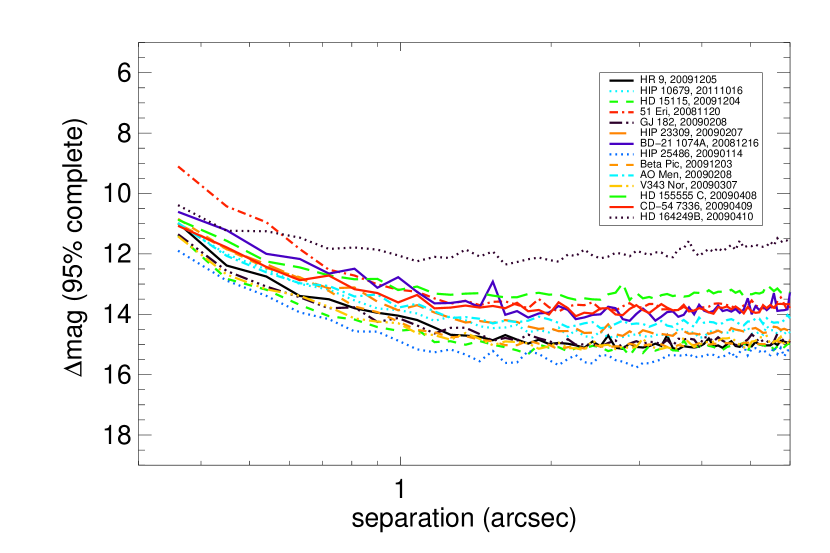
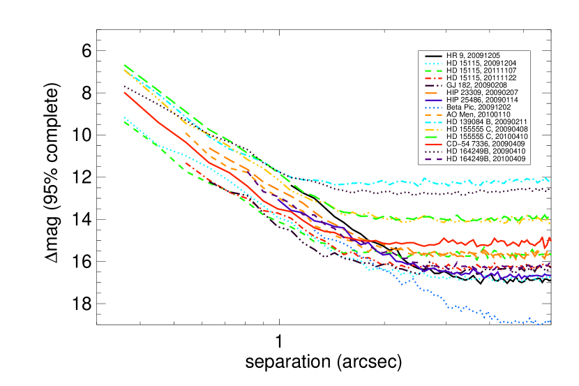
Figure 4: 95% completeness contrast curves for $\beta$ Pic moving group stars (1st half), with plot range from 0.3” (coronagraph inner working angle) to 6”. Top: ASDI contrasts. Bottom: ADI contrasts.

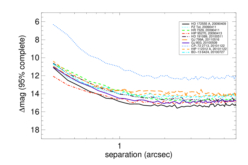
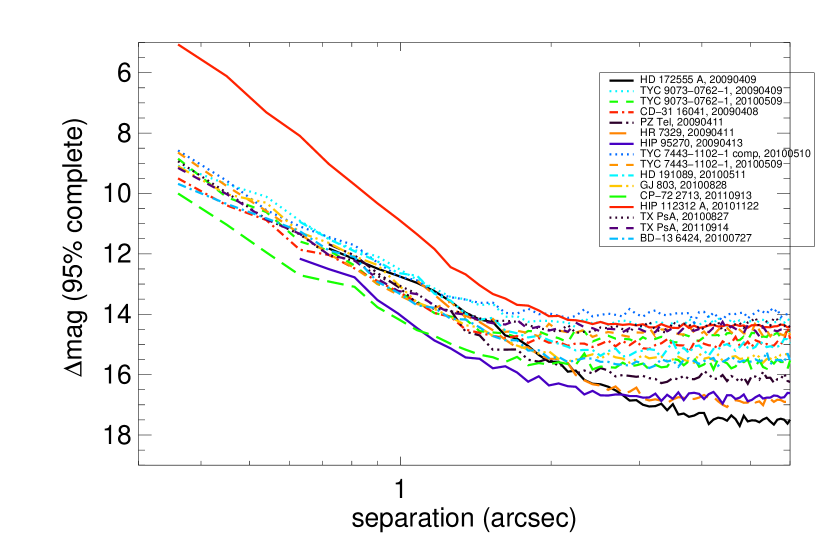
Figure 5: 95% completeness contrast curves for $\beta$ moving group (2nd half), with plot range from 0.3” (coronagraph inner working angle) to 6”. Top: ASDI contrasts. Bottom: ADI contrasts.

Figure 6: 95% completeness contrast curves for Tucana-Horologium association stars, with plot range from 0.3” (coronagraph inner working angle) to 6”. Top: ASDI contrasts. Bottom: ADI contrasts.

Figure 7: 95% completeness contrast curves for AB Dor moving group stars, with plot range from 0.3” (coronagraph inner working angle) to 6”. Top: ASDI contrasts. Bottom: ADI contrasts.

Figure 8: 95% completeness contrast curves for Hercules-Lyra association stars, with plot range from 0.3” (coronagraph inner working angle) to 6”. Top: ASDI contrasts. Bottom: ADI contrasts.

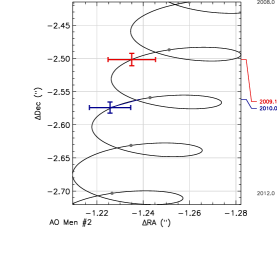
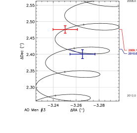
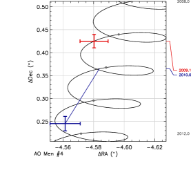
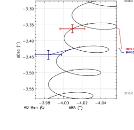
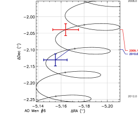
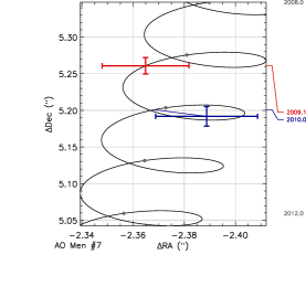
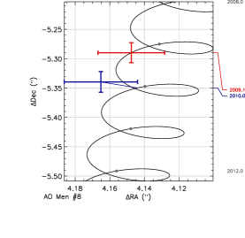
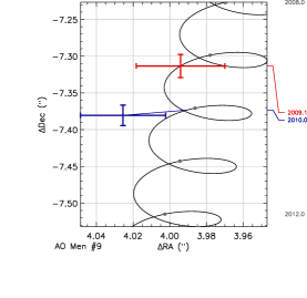
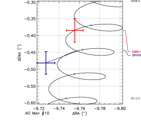
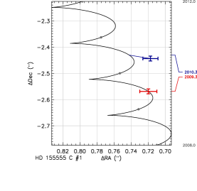
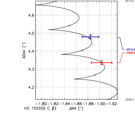
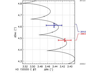
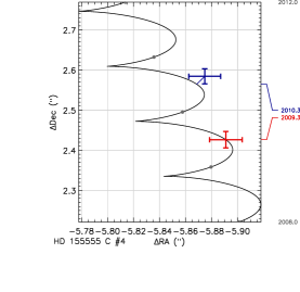
Figure 12: On-sky plots for $\beta$ Pic MG objects.

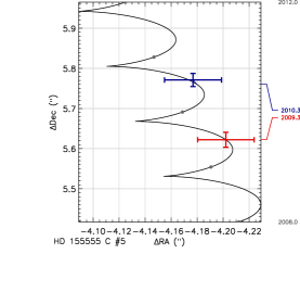
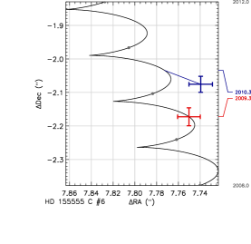
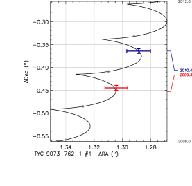
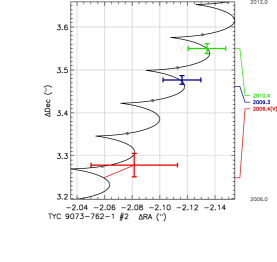
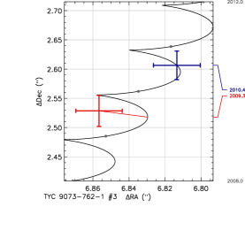
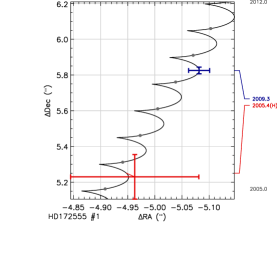
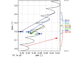
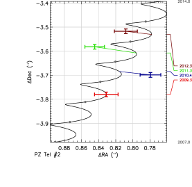
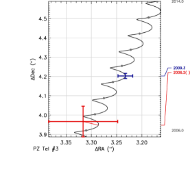
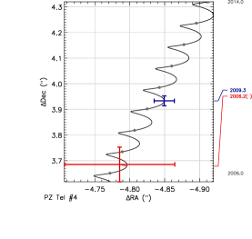
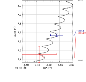
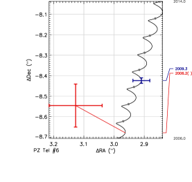
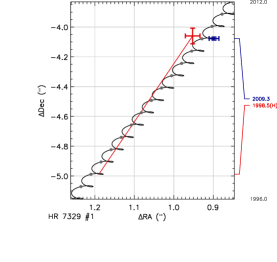
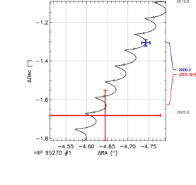
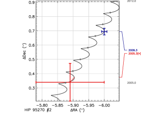
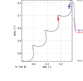
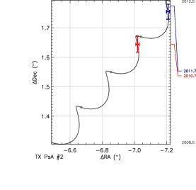
Figure 13: On-sky plots for $\beta$ Pic MG objects (continued).

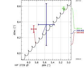
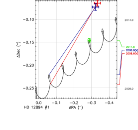
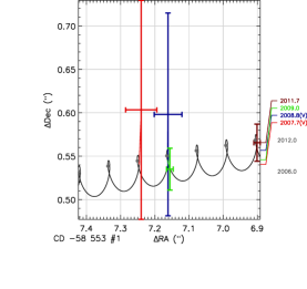
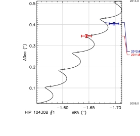
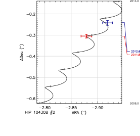
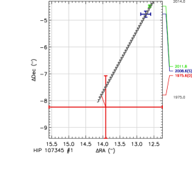
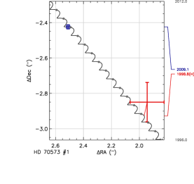
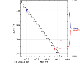
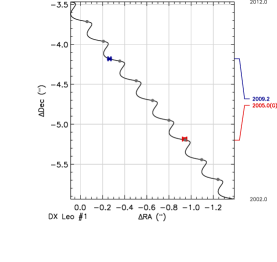
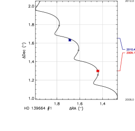
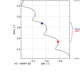
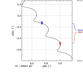
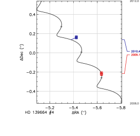
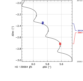
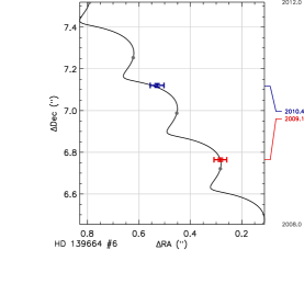
Figure 14: On-sky plots for Tucana-Horologium and Hercules-Lyra association objects.

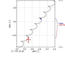
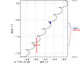
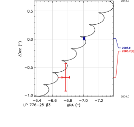
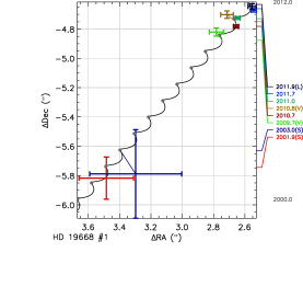
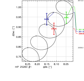
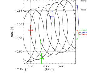
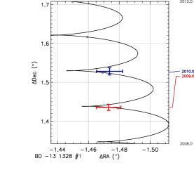
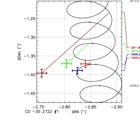
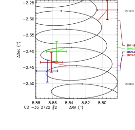
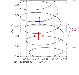
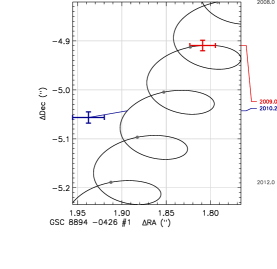
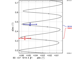
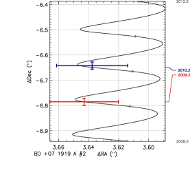
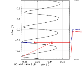
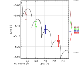
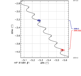
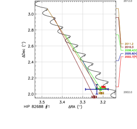
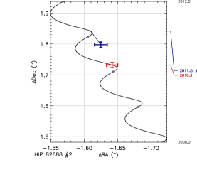
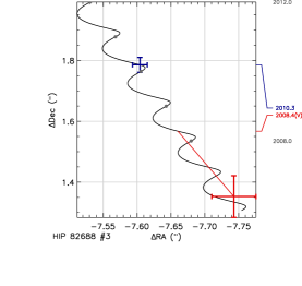
Figure 15: On-Sky plots for AB Dor MG objects.

$\beta$ Pic b only

AB Pic B only

$\beta$ Pic b and AB Pic B

Figure 23: Comparison of 1-d marginalized posterior pdfs including (left) only the $\beta$ Pic b detection, (center) only the AB Pic B detection, and (right) both detections. Posterior probability is plotted in logarithmic units. For AB Pic B, in the case of small ($<$50 AU) cutoffs, ln(PDF) trended to negative infinity and is not plotted here.

Appendix A Candidate companions observed at only one epoch

By the end of NICI Campaign observations, we were unable to obtain followup observations for a number of candidate companions at projected separations $>$400 AU or in dense stellar fields ($>$20 objects in the field) located in the Galactic bulge or disk. Here we list target stars with candidate companions for which we only have a single epoch of data. Since we cannot classify these as either CPM or background, we provide the properties of these candidates here and note the changes we make to the contrast curves in the Action column. Contrast curves are edited either by reverting to a less sensitive contrast curve or restricting the contrast curve to within a given separation. For cases where we have only a single epoch and there are candidates inside the 100% coverage region for position angle, we drop the star from our analysis.

Table 17: Candidate Companions with One Epoch of Data

Star	#	Sep	Sep	PA	$\Delta H$	Epoch	Action
		(“)	(AU)	(deg)	(mag)
AO Men	1	4.74	183	108.1	15.6	2009.1041	Revert to 2009.10 ASDI
	2	6.87	264	32.1	15.6	2009.1041
	3	6.92	266	102.4	14.7	2009.1041
	4	7.86	303	65.4	15.2	2009.1041
CD-54 7336	1	2.92	193	252.5	8.1	2009.2684	Drop
	2	4.26	281	228.6	15.0	2009.2684
	3	4.32	285	27.7	10.6	2009.2684
	4	4.74	313	207.1	13.2	2009.2684
	5	5.39	356	264.5	14.1	2009.2684
	6	6.28	415	132.0	11.6	2009.2684
	7	6.36	420	100.6	5.7	2009.2684
	8	6.55	433	332.6	14.6	2009.2684
	9	6.95	459	296.6	13.3	2009.2684
	10	7.04	465	167.6	11.5	2009.2684
	11	7.15	472	91.6	11.7	2009.2684
	12	7.68	507	105.5	11.1	2009.2684
	13	8.17	539	284.1	13.4	2009.2684
	14	8.24	544	346.0	13.2	2009.2684
	15	8.67	572	100.1	14.7	2009.2684
CD-31 16041	1	1.94	99	65.3	11.7	2009.2657	Drop
	2	2.59	132	87.2	12.9	2009.2657
	3	3.12	159	123.5	14.2	2009.2657
	4	3.47	177	176.1	11.1	2009.2657
	5	3.60	184	156.5	11.8	2009.2657
	6	3.62	185	12.0	14.8	2009.2657
	7	3.63	185	174.3	14.6	2009.2657
	8	3.69	188	160.7	15.1	2009.2657
	9	3.69	188	16.7	10.9	2009.2657
	10	3.89	199	111.4	14.4	2009.2657
	11	4.45	227	188.1	12.1	2009.2657
	12	4.50	229	71.1	14.0	2009.2657
	13	4.85	247	115.4	14.8	2009.2657
	14	5.01	256	65.0	10.7	2009.2657
	15	5.09	260	77.6	12.8	2009.2657
	16	5.13	262	69.1	14.9	2009.2657
	17	5.61	286	273.7	13.6	2009.2657
	18	5.62	287	201.2	12.2	2009.2657
	19	5.77	294	77.6	14.7	2009.2657
	20	5.85	298	345.2	14.2	2009.2657
	21	6.01	307	282.4	14.0	2009.2657
	22	6.50	332	16.0	13.1	2009.2657
	23	6.79	346	235.9	15.0	2009.2657
	24	6.87	350	177.0	12.1	2009.2657
	25	7.12	363	249.0	13.1	2009.2657
	26	7.92	404	90.4	14.3	2009.2657
	27	8.09	413	326.3	13.7	2009.2657
	28	8.35	426	72.7	14.6	2009.2657
	29	8.42	430	3.8	14.5	2009.2657
	30	8.98	458	340.4	13.2	2009.2657
	31	9.12	465	76.2	11.4	2009.2657
	32	9.17	468	37.4	14.8	2009.2657
	33	9.32	475	74.1	11.2	2009.2657
	34	10.05	512	328.5	13.2	2009.2657
HD 159911	1	3.79	171	118.3	13.8	2010.2712	Drop
	2	3.99	179	79.1	10.7	2010.2712
	3	4.86	219	288.3	14.0	2010.2712
	4	4.95	223	315.9	13.3	2010.2712
	5	5.24	236	159.3	13.1	2010.2712
	6	5.35	241	315.1	11.2	2010.2712
	7	5.74	258	343.1	10.5	2010.2712
	8	5.75	259	357.5	12.5	2010.2712
	9	5.79	261	259.3	13.2	2010.2712
	10	6.24	281	165.8	12.9	2010.2712
	11	6.27	282	248.5	14.8	2010.2712
	12	7.14	321	287.0	11.3	2010.2712
	13	7.23	326	248.6	12.8	2010.2712
	14	7.67	345	18.6	8.0	2010.2712
TYC 7443-1102-1A	1	7.94	458	155.4	12.3	2010.3507	Sep $<$ 7.94”
	2	8.89	513	355.0	13.6	2010.3507
TYC 7443-1102-1B	1	8.85	511	12.7	12.8	2010.3534	Sep $<$ 8.85”
GJ 560 A	1	5.71	94	230.7	15.9	2009.1891	Sep $<$ 5.88”
	2	5.88	96	185.6	15.8	2009.1891
	3	6.15	101	27.5	16.3	2009.1891
	4	6.30	103	52.6	16.1	2009.1891
	5	6.86	113	269.0	14.6	2009.1891
	6	7.34	120	284.4	15.0	2009.1891
HD 139664	1	4.49	79	241.6	16.2	2010.3507	Revert to 2009.10 ASDI
	2	5.19	91	311.6	17.2	2010.3507
	3	6.08	106	335.6	15.8	2010.3507
	4	6.45	113	310.0	16.8	2010.3507
	5	7.04	123	16.6	15.8	2010.3507
	6	8.48	148	68.1	15.7	2010.3507
	7	9.13	160	301.2	15.2	2010.3507
	8	10.55	185	37.7	16.7	2010.3507
HD 92945	1	8.43	182	253.4	15.9	2009.0383	Sep $<$ 8.43”
TYC 9073-762-1	1	8.01	433	27.9	16.7	2010.3507	No Change
	2	9.31	503	-78.2	15.4	2010.3507
GSC 8894-0426	1	9.93	228	-118.2	9.6	2010.1589	Sep $<$ 9.93”
HD 164249B	1	4.60	216	136.3	12.6	2009.2712	Sep $<$ 6.27”, Revert to 2009.27 ASDI
	2	6.27	295	80.9	7.0	2009.2712
	3	7.72	363	58.1	12.9	2009.2712
	4	8.27	389	36.5	10.2	2009.2712
HR 4796 B	1	8.86	595	103.4	11.8	2009.1151	Sep $<$ 8.86”
V343 Nor	1	1.32	53	317.2	14.6	2009.1781	Drop
	2	1.77	70	170.6	12.8	2009.1781
	3	1.81	72	15.6	13.9	2009.1781
	4	1.91	76	330.1	14.0	2009.1781
	5	2.08	83	251.9	14.8	2009.1781
	6	2.16	86	108.9	15.5	2009.1781
	7	2.30	91	198.7	9.1	2009.1781
	8	2.41	96	188.1	12.3	2009.1781
	9	2.49	99	195.0	13.8	2009.1781
	10	2.61	104	251.9	16.1	2009.1781
	11	2.67	106	71.2	13.7	2009.1781
	12	2.69	107	324.0	15.9	2009.1781
	13	2.93	117	131.0	13.5	2009.1781
	14	2.93	117	45.2	13.8	2009.1781
	15	3.04	121	86.6	14.0	2009.1781
	16	3.04	121	350.1	8.8	2009.1781
	17	3.07	122	169.2	15.8	2009.1781
	18	3.09	123	91.7	15.7	2009.1781
	19	3.27	130	51.2	15.0	2009.1781
	20	3.33	132	27.0	15.8	2009.1781
	21	3.34	133	206.2	12.5	2009.1781
	22	3.38	135	86.7	15.8	2009.1781
	23	3.67	146	11.6	13.6	2009.1781
	24	3.76	150	33.3	13.9	2009.1781
	25	3.77	150	257.4	10.2	2009.1781
	26	3.78	150	331.6	14.1	2009.1781
	27	3.83	152	18.6	13.7	2009.1781
	28	3.91	156	293.9	11.8	2009.1781
	29	3.96	157	54.8	13.2	2009.1781
	30	4.14	165	110.3	12.0	2009.1781
	31	4.22	168	11.5	13.9	2009.1781
	32	4.25	169	80.0	7.8	2009.1781
	33	4.28	170	328.0	14.6	2009.1781
	34	4.30	171	93.4	15.1	2009.1781
	35	4.41	175	95.8	14.9	2009.1781
	36	4.45	177	148.9	12.3	2009.1781
	37	4.48	178	237.3	14.3	2009.1781
	38	4.52	180	356.1	15.3	2009.1781
	39	4.58	182	205.1	11.2	2009.1781
	40	4.62	184	133.4	15.5	2009.1781
	41	4.67	186	334.7	15.2	2009.1781
	42	4.69	187	27.4	14.6	2009.1781
	43	4.73	188	196.3	12.3	2009.1781
	44	4.74	189	212.0	10.7	2009.1781
	45	4.77	190	102.6	11.5	2009.1781
	46	4.80	191	136.5	13.1	2009.1781
	47	4.82	192	181.7	14.8	2009.1781
	48	4.86	193	26.1	15.2	2009.1781
	49	4.88	194	309.0	14.7	2009.1781
	50	4.91	195	319.6	14.3	2009.1781
	51	4.93	196	272.5	12.4	2009.1781
	52	4.93	196	314.7	12.8	2009.1781
	53	4.94	196	230.5	14.3	2009.1781
	54	5.01	199	359.8	13.9	2009.1781
	55	5.18	206	237.7	14.9	2009.1781
	56	5.23	208	291.5	13.7	2009.1781
	57	5.24	208	308.9	15.1	2009.1781
	58	5.39	214	155.6	15.3	2009.1781
	59	5.39	215	295.5	11.3	2009.1781
	60	5.42	216	210.9	15.0	2009.1781
	61	5.45	217	229.3	15.6	2009.1781
	62	5.46	217	239.6	15.4	2009.1781
	63	5.48	218	127.5	14.2	2009.1781
	64	5.53	220	335.4	8.8	2009.1781
	65	5.55	221	196.6	15.3	2009.1781
	66	5.60	223	313.8	12.6	2009.1781
	67	5.63	224	354.5	14.2	2009.1781
	68	5.65	225	164.5	14.7	2009.1781
	69	5.74	228	165.9	15.0	2009.1781
	70	5.76	229	331.1	14.0	2009.1781
	71	5.83	232	201.5	11.9	2009.1781
	72	5.84	233	232.7	15.7	2009.1781
	73	5.87	234	81.4	13.8	2009.1781
	74	5.94	236	94.0	13.9	2009.1781
	75	5.95	237	191.1	13.5	2009.1781
	76	5.96	237	306.7	12.9	2009.1781
	77	6.07	241	149.2	12.1	2009.1781
	78	6.08	242	312.6	14.6	2009.1781
	79	6.09	242	336.5	15.4	2009.1781
	80	6.10	243	60.6	12.0	2009.1781
	81	6.17	246	102.9	15.7	2009.1781
	82	6.21	247	107.5	13.5	2009.1781
	83	6.23	248	330.8	14.3	2009.1781
	84	6.25	249	209.4	14.1	2009.1781
	85	6.26	249	288.2	13.7	2009.1781
	86	6.36	253	116.5	15.7	2009.1781
	87	6.42	255	59.6	10.5	2009.1781
	88	6.47	258	202.9	14.1	2009.1781
	89	6.53	260	202.1	14.6	2009.1781
	90	6.53	260	3.9	15.3	2009.1781
	91	6.55	261	226.6	15.1	2009.1781
	92	6.57	261	325.7	15.2	2009.1781
	93	6.63	264	105.2	15.4	2009.1781
	94	6.67	265	248.3	13.5	2009.1781
	95	6.67	266	40.6	13.6	2009.1781
	96	6.68	266	121.5	15.3	2009.1781
	97	6.71	267	70.8	9.0	2009.1781
	98	6.71	267	9.2	14.5	2009.1781
	99	6.75	269	230.7	13.9	2009.1781
	100	6.77	269	185.6	10.5	2009.1781
	101	6.80	271	85.0	15.7	2009.1781
	102	6.85	273	353.4	13.8	2009.1781
	103	6.86	273	292.1	15.3	2009.1781
	104	6.89	274	279.8	13.7	2009.1781
	105	6.98	278	84.8	15.3	2009.1781
	106	7.14	284	182.5	14.4	2009.1781
	107	7.17	285	148.1	13.5	2009.1781
	108	7.25	289	37.6	12.9	2009.1781
	109	7.26	289	269.4	14.1	2009.1781
	110	7.28	290	300.6	14.2	2009.1781
	111	7.35	292	89.6	12.8	2009.1781
	112	7.41	295	92.8	13.4	2009.1781
	113	7.46	297	257.8	13.9	2009.1781
	114	7.48	298	80.9	12.5	2009.1781
	115	7.63	304	297.5	9.1	2009.1781
	116	7.74	308	201.9	13.6	2009.1781
	117	7.77	309	112.1	12.2	2009.1781
	118	7.85	312	204.0	12.3	2009.1781
	119	7.96	317	24.3	13.8	2009.1781
HD 139084 B	1	0.92	37	206.6	8.1	2009.1123	Drop
	2	1.19	48	347.8	9.5	2009.1123
	3	1.38	55	119.6	11.2	2009.1123
	4	1.51	60	32.4	12.3	2009.1123
	5	1.78	71	351.3	12.1	2009.1123
	6	1.84	73	241.4	11.1	2009.1123
	7	1.96	78	355.3	11.6	2009.1123
	8	2.11	84	258.7	9.4	2009.1123
	9	2.22	88	14.0	11.3	2009.1123
	10	2.23	89	267.2	11.4	2009.1123
	11	2.26	90	226.3	7.3	2009.1123
	12	2.39	95	57.3	9.3	2009.1123
	13	2.43	97	241.7	11.7	2009.1123
	14	2.45	97	302.4	9.8	2009.1123
	15	2.73	109	290.8	11.9	2009.1123
	16	2.79	111	326.0	10.0	2009.1123
	17	2.82	112	39.6	6.2	2009.1123
	18	2.85	113	26.6	11.7	2009.1123
	19	2.86	114	129.4	12.0	2009.1123
	20	2.88	115	303.3	11.9	2009.1123
	21	3.02	120	183.7	9.8	2009.1123
	22	3.45	137	335.7	11.8	2009.1123
	23	3.60	143	188.6	9.7	2009.1123
	24	3.62	144	83.4	11.4	2009.1123
	25	3.69	147	198.4	10.7	2009.1123
	26	3.72	148	192.6	12.2	2009.1123
	27	3.77	150	139.6	11.6	2009.1123
	28	3.87	154	23.2	10.3	2009.1123
	29	3.98	158	8.8	11.0	2009.1123
	30	4.06	162	210.9	11.6	2009.1123
	31	4.17	166	182.7	12.3	2009.1123
	32	4.22	168	132.6	10.6	2009.1123
	33	4.30	171	60.4	9.6	2009.1123
	34	4.46	178	6.0	10.6	2009.1123
	35	4.48	178	158.4	11.1	2009.1123
	36	4.56	182	181.4	11.0	2009.1123
	37	4.65	185	134.4	10.5	2009.1123
	38	4.66	186	194.7	11.5	2009.1123
	39	4.80	191	268.3	9.2	2009.1123
	40	4.85	193	310.9	11.2	2009.1123
	41	4.88	194	154.9	9.0	2009.1123
	42	4.91	195	164.1	9.3	2009.1123
	43	5.03	200	203.5	10.5	2009.1123
	44	5.04	201	130.7	5.0	2009.1123
	45	5.08	202	248.9	9.8	2009.1123
	46	5.13	204	289.6	9.3	2009.1123
	47	5.16	205	310.6	11.2	2009.1123
	48	5.27	210	210.1	11.7	2009.1123
	49	5.36	213	22.4	10.1	2009.1123
	50	5.38	214	326.3	10.4	2009.1123
	51	5.38	214	25.1	9.1	2009.1123
	52	5.40	215	158.1	11.9	2009.1123
	53	5.42	216	147.3	10.8	2009.1123
	54	5.47	218	82.3	10.5	2009.1123
	55	5.50	219	151.9	9.3	2009.1123
	56	5.56	221	105.7	9.8	2009.1123
	57	5.58	222	345.7	9.9	2009.1123
	58	5.58	222	228.0	5.9	2009.1123
	59	5.65	225	333.8	8.8	2009.1123
	60	5.66	225	27.4	10.4	2009.1123
	61	5.67	226	260.1	8.5	2009.1123
	62	5.70	227	182.5	12.0	2009.1123
	63	5.72	228	340.9	11.6	2009.1123
	64	5.74	228	277.4	12.0	2009.1123
	65	5.76	229	237.6	11.4	2009.1123
	66	5.83	232	43.4	10.8	2009.1123
	67	5.90	235	77.5	9.7	2009.1123
	68	6.00	239	269.7	9.8	2009.1123
	69	6.02	240	60.5	8.3	2009.1123
	70	6.05	241	140.8	11.2	2009.1123
	71	6.10	243	168.5	7.8	2009.1123
	72	6.13	244	328.2	11.1	2009.1123

Note. — Target stars with candidate companions for which we only have a single epoch of data. Since we cannot classify these as either CPM or background, we provide the properties of these candidates here and note the changes we make to the contrast curves in the Action column. Contrast curves are edited either by reverting to a less sensitive contrast curve or restricting the contrast curve to within a given separation. For cases where we have only a single epoch and there are candidates inside the 100% coverage region for position angle, we drop the star from our analysis.

References

- Allen (2007) Allen, P. R. 2007, ApJ, 668, 492
- Allers & Liu (2013) Allers, K. N., & Liu, M. C. 2013, ApJ, 772, 79
- Apai et al. (2008) Apai, D., Janson, M., Moro-Martín, A., et al. 2008, ApJ, 672, 1196
- Barrado y Navascués et al. (1999) Barrado y Navascués, D., Stauffer, J. R., Song, I., & Caillault, J.-P. 1999, ApJ, 520, L123
- Barrado Y Navascués (2006) Barrado Y Navascués, D. 2006, A&A, 459, 511
- Baraffe et al. (1998) Baraffe, I., Chabrier, G., Allard, F., & Hauschildt, P. H. 1998, A&A, 337, 403
- Baraffe et al. (2002) Baraffe, I., Chabrier, G., Allard, F., & Hauschildt, P. H. 2002, A&A, 382, 563
- Baraffe et al. (2003) Baraffe, I., Chabrier, G., Barman, T. S., Allard, F., & Hauschildt, P. H. 2003, A&A, 402, 701
- Barman et al. (2011a) Barman, T. S., Macintosh, B., Konopacky, Q. M., & Marois, C. 2011, ApJ, 733, 65
- Barman et al. (2011b) Barman, T. S., Macintosh, B., Konopacky, Q. M., & Marois, C. 2011, ApJ, 735, L39
- Biller et al. (2007) Biller, B. A., Close, L. M., Masciadri, E., et al. 2007, ApJS, 173, 143
- Biller et al. (2008) Biller, B., Artigau, É., Wahhaj, Z., et al. 2008, Proc. SPIE, 7015,
- Biller et al. (2010) Biller, B. A., Liu, M. C., Wahhaj, Z., et al. 2010, ApJ, 720, L82
- Bonavita et al. (2012) Bonavita, M., Chauvin, G., Desidera, S., et al. 2012, A&A, 537, A67
- Bonnefoy et al. (2010) Bonnefoy, M., Chauvin, G., Rojo, P., et al. 2010, A&A, 512, A52
- Bonnefoy et al. (2013) Bonnefoy, M., Boccaletti, A., Lagrange, A.-M., et al. 2013, arXiv:1302.1160
- Bowler et al. (2010) Bowler, B. P., Liu, M. C., Dupuy, T. J., & Cushing, M. C. 2010, ApJ, 723, 850
- Bowler et al. (2013) Bowler, B. P., Liu, M. C., Shkolnik, E. L., & Dupuy, T. J. 2013, arXiv:1307.2237
- Buenzli et al. (2010) Buenzli, E., Thalmann, C., Vigan, A., et al. 2010, A&A, 524, L1
- Burrows et al. (2003) Burrows, A., Sudarsky, D., & Lunine, J. I. 2003, ApJ, 596, 587
- Carson et al. (2013) Carson, J., Thalmann, C., Janson, M., et al. 2012, arXiv:1211.3744
- Chabrier et al. (2000) Chabrier, G., Baraffe, I., Allard, F., & Hauschildt, P. 2000, ApJ, 542, 464
- Chauvin et al. (2005a) Chauvin, G., Lagrange, A.-M., Dumas, C., et al. 2005, A&A, 438, L25
- Chauvin et al. (2005b) Chauvin, G., Lagrange, A.-M., Zuckerman, B., et al. 2005, A&A, 438, L29
- Chauvin et al. (2010) Chauvin, G., Lagrange, A.-M., Bonavita, M., et al. 2010, A&A, 509, A52
- Chauvin et al. (2012) Chauvin, G., Lagrange, A.-M., Beust, H., et al. 2012, A&A, 542, A41
- Close et al. (2005) Close, L. M., Lenzen, R., Guirado, J. C., et al. 2005, Nature, 433, 286
- Close et al. (2007) Close, L. M., Thatte, N., Nielsen, E. L., et al. 2007, ApJ, 665, 736
- Close & Males (2010) Close, L. M., & Males, J. R. 2010, ApJ, 709, 342
- Chun et al. (2008) Chun, M., Toomey, D., Wahhaj, Z., et al. 2008, Proc. SPIE, 7015,
- Currie et al. (2011) Currie, T., Thalmann, C., Matsumura, S., et al. 2011, ApJ, 736, L33
- Cumming et al. (2008) Cumming, A., Butler, R. P., Marcy, G. W., et al. 2008, PASP, 120, 531
- Cushing et al. (2005) Cushing, M. C., Rayner, J. T., & Vacca, W. D. 2005, ApJ, 623, 1115
- da Silva et al. (2009) da Silva, L., Torres, C. A. O., de La Reza, R., et al. 2009, A&A, 508, 833
- de la Reza et al. (1989) de la Reza, R., Torres, C. A. O., Quast, G., Castilho, B. V., & Vieira, G. L. 1989, ApJ, 343, L61
- Delorme et al. (2013) Delorme, P., Gagné, J., Girard, J. H., et al. 2013, A&A, 553, L5
- Dodson-Robinson et al. (2009) Dodson-Robinson, S. E., Veras, D., Ford, E. B., & Beichman, C. A. 2009, ApJ, 707, 79
- Dommanget & Nys (2002) Dommanget, J., & Nys, O. 2002, VizieR Online Data Catalog, 1274, 0
- Dupuy et al. (2010) Dupuy, T. J., Liu, M. C., Bowler, B. P., et al. 2010, ApJ, 721, 1725
- Dupuy & Liu (2011) Dupuy, T. J. & Liu, M. C. 2011, ApJ, 733, 122
- Dupuy & Liu (2012) Dupuy, T. J. & Liu, M. C. 2012, ApJS, 201, 19
- Fernández et al. (2008) Fernández, D., Figueras, F., & Torra, J. 2008, A&A, 480, 735
- Fischer & Valenti (2005) Fischer, D. A., & Valenti, J. 2005, ApJ, 622, 1102
- Fuhrmann (2004) Fuhrmann, K. 2004, Astronomische Nachrichten, 325, 3
- Gaidos (1998) Gaidos, E. J. 1998, PASP, 110, 1259
- Geballe et al. (2002) Geballe, T. R., Knapp, G. R., Leggett, S. K., et al. 2002, ApJ, 564, 466
- Gizis (2002) Gizis, J. E. 2002, ApJ, 575, 484
- Gray et al. (2006) Gray, R. O., Corbally, C. J., Garrison, R. F., et al. 2006, AJ, 132, 161
- Gregorio-Hetem et al. (1992) Gregorio-Hetem, J., Lepine, J. R. D., Quast, G. R., Torres, C. A. O., & de La Reza, R. 1992, AJ, 103, 549
- Guenther et al. (2001) Guenther, E. W., Neuhäuser, R., Huélamo, N., Brandner, W., & Alves, J. 2001, A&A, 365, 514
- Guirado et al. (1997) Guirado, J. C., Reynolds, J. E., Lestrade, J.-F., et al. 1997, ApJ, 490, 835
- Heinze et al. (2010a) Heinze, A. N., Hinz, P. M., Sivanandam, S., et al. 2010, ApJ, 714, 1551
- Heinze et al. (2010b) Heinze, A. N., Hinz, P. M., Kenworthy, M., et al. 2010, ApJ, 714, 1570
- Høg et al. (2000) Høg, E., Fabricius, C., Makarov, V. V., et al. 2000, A&A, 355, L27
- Ireland et al. (2011) Ireland, M. J., Kraus, A., Martinache, F., Law, N., & Hillenbrand, L. A. 2011, ApJ, 726, 113
- Janson et al. (2011) Janson, M., Bonavita, M., Klahr, H., et al. 2011, ApJ, 736, 89
- Janson et al. (2012) Janson, M., Bonavita, M., Klahr, H., & Lafrenière, D. 2012, ApJ, 745, 4
- Jayawardhana et al. (1999) Jayawardhana, R., Hartmann, L., Fazio, G., et al. 1999, ApJ, 521, L129
- Johnson et al. (2007) Johnson, J. A., Butler, R. P., Marcy, G. W., et al. 2007, ApJ, 670, 833
- Johnson et al. (2010) Johnson, J. A., Aller, K. M., Howard, A. W., & Crepp, J. R. 2010, PASP, 122, 905
- Kalas et al. (2008) Kalas, P., Graham, J. R., Chiang, E., et al. 2008, Science, 322, 1345
- Kasper et al. (2007) Kasper, M., Apai, D., Janson, M., & Brandner, W. 2007, A&A, 472, 321
- Kastner et al. (1997) Kastner, J. H., Zuckerman, B., Weintraub, D. A., & Forveille, T. 1997, Science, 277, 67
- Kastner et al. (2008) Kastner, J. H., Zuckerman, B., & Bessell, M. 2008, A&A, 491, 829
- Kenyon & Hartmann (1995) Kenyon, S. J., & Hartmann, L. 1995, ApJS, 101, 117
- Kiss et al. (2011) Kiss, L. L., Moór, A., Szalai, T., et al. 2011, MNRAS, 411, 117
- Koen et al. (2010) Koen, C., Kilkenny, D., van Wyk, F., & Marang, F. 2010, MNRAS, 403, 1949
- Kraus et al. (2011) Kraus, A. L., Ireland, M. J., Martinache, F., & Hillenbrand, L. A. 2011, ApJ, 731, 8
- Kraus & Ireland (2012) Kraus, A. L., & Ireland, M. J. 2012, ApJ, 745, 5
- Kuzuhara et al. (2013) Kuzuhara, M., Tamura, M., Kudo, T., et al. 2013, accepted to ApJ, arXiv:1307.2886
- Lafrenière et al. (2007a) Lafrenière, D., Marois, C., Doyon, R., Nadeau, D., & Artigau, É. 2007, ApJ, 660, 770
- Lafrenière et al. (2007b) Lafrenière, D., Doyon, R., Marois, C., et al. 2007, ApJ, 670, 1367
- Lafrenière et al. (2008) Lafrenière, D., Jayawardhana, R., & van Kerkwijk, M. H. 2008, ApJ, 689, L153
- Lagrange et al. (2009) Lagrange, A.-M., Gratadour, D., Chauvin, G., et al. 2009, A&A, 493, L21
- Lagrange et al. (2010) Lagrange, A.-M., Bonnefoy, M., Chauvin, G., et al. 2010, Science, 329, 57
- Landolt (2009) Landolt, A. U. 2009, AJ, 137, 4186
- Lépine & Simon (2009) Lépine, S., & Simon, M. 2009, AJ, 137, 3632
- Liu (2004) Liu, M. C. 2004, Science, 305, 1442
- Liu et al. (2010) Liu, M. C., Wahhaj, Z., Biller, B. A., et al. 2010, Proc. SPIE, 7736,
- Looper et al. (2007) Looper, D. L., Burgasser, A. J., Kirkpatrick, J. D., & Swift, B. J. 2007, ApJ, 669, L97
- Looper et al. (2010a) Looper, D. L., Bochanski, J. J., Burgasser, A. J., et al. 2010, AJ, 140, 1486
- Looper et al. (2010b) Looper, D. L., Mohanty, S., Bochanski, J. J., et al. 2010, ApJ, 714, 45
- López-Santiago et al. (2006) López-Santiago, J., Montes, D., Crespo-Chacón, I., & Fernández-Figueroa, M. J. 2006, ApJ, 643, 1160
- Lowrance et al. (2000) Lowrance, P. J., Schneider, G., Kirkpatrick, J. D., et al. 2000, ApJ, 541, 390
- Lowrance et al. (2005) Lowrance, P. J., Becklin, E. E., Schneider, G., et al. 2005, AJ, 130, 1845
- Luhman et al. (2005) Luhman, K. L., Stauffer, J. R., & Mamajek, E. E. 2005, ApJ, 628, L69
- Luhman et al. (2011) Luhman, K. L., Burgasser, A. J., & Bochanski, J. J. 2011, ApJ, 730, L9
- Mamajek (2005) Mamajek, E. E. 2005, ApJ, 634, 1385
- Malo et al. (2013) Malo, L., Doyon, R., Lafrenière, D., et al. 2013, ApJ, 762, 88
- Marois et al. (2005) Marois, C., Doyon, R., Nadeau, D., et al. 2005, PASP, 117, 745
- Marois et al. (2006) Marois, C., Lafrenière, D., Doyon, R., Macintosh, B., & Nadeau, D. 2006, ApJ, 641, 556
- Marois et al. (2008) Marois, C., Macintosh, B., Barman, T., et al. 2008, Science, 322, 1348
- Marois et al. (2010) Marois, C., Zuckerman, B., Konopacky, Q. M., Macintosh, B., & Barman, T. 2010, Nature, 468, 1080
- Masciadri et al. (2005) Masciadri, E., Mundt, R., Henning, T., Alvarez, C., & Barrado y Navascués, D. 2005, ApJ, 625, 1004
- Mason et al. (2013) Mason, B. D., Wycoff, G. L., Hartkopf, W. I., Douglass, G. G., & Worley, C. E. 2013, VizieR Online Data Catalog, 1, 2026
- Messina et al. (2010) Messina, S., Desidera, S., Turatto, M., Lanzafame, A. C., & Guinan, E. F. 2010, A&A, 520, A15
- Metchev & Hillenbrand (2009) Metchev, S. A., & Hillenbrand, L. A. 2009, ApJS, 181, 62
- Montes et al. (2001) Montes, D., López-Santiago, J., Fernández-Figueroa, M. J., & Gálvez, M. C. 2001, A&A, 379, 976
- Mordasini et al. (2009) Mordasini, C., Alibert, Y., & Benz, W. 2009, A&A, 501, 1139
- Moór et al. (2006) Moór, A., Ábrahám, P., Derekas, A., et al. 2006, ApJ, 644, 525
- Mugrauer et al. (2012) Mugrauer, M., Röll, T., Ginski, C., et al. 2012, MNRAS, 424, 1714
- Nielsen et al. (2005) Nielsen, E. L., Close, L. M., Guirado, J. C., et al. 2005, Astronomische Nachrichten, 326, 1033
- Nielsen et al. (2008) Nielsen, E. L., Close, L. M., Biller, B. A., Masciadri, E., & Lenzen, R. 2008, ApJ, 674, 466
- Nielsen & Close (2010) Nielsen, E. L., & Close, L. M. 2010, ApJ, 717, 878
- Nielsen et al. (2012) Nielsen, E. L., Liu, M. C., Wahhaj, Z., et al. 2012, ApJ, 750, 53
- Nielsen et al. (2013) Nielsen, E. L., Liu, M. C., Wahhaj, Z., et al. 2013, accepted to ApJ, arXiv:1306.1233
- Quanz et al. (2013) Quanz, S. P., Amara, A., Meyer, M. R., et al. 2013, ApJ, 766, L1
- Racine et al. (1999) Racine, R., Walker, G. A. H., Nadeau, D., Doyon, R., & Marois, C. 1999, PASP, 111, 587
- Rameau et al. (2013a) Rameau, J., Chauvin, G., Lagrange, A.-M., et al. 2013, A&A, 553, A60
- Rameau et al. (2013) Rameau, J., Chauvin, G., Lagrange, A.-M., et al. 2013, arXiv:1305.7428
- Rebull et al. (2008) Rebull, L. M., Stapelfeldt, K. R., Werner, M. W., et al. 2008, ApJ, 681, 1484
- Riaz et al. (2006) Riaz, B., Gizis, J. E., & Harvin, J. 2006, AJ, 132, 866
- Rice et al. (2010) Rice, E. L., Faherty, J. K., & Cruz, K. L. 2010, ApJ, 715, L165
- Rodriguez et al. (2011) Rodriguez, D. R., Bessell, M. S., Zuckerman, B., & Kastner, J. H. 2011, ApJ, 727, 62
- Rucinski & Krautter (1983) Rucinski, S. M., & Krautter, J. 1983, A&A, 121, 217
- Schlieder et al. (2010) Schlieder, J. E., Lépine, S., & Simon, M. 2010, AJ, 140, 119
- Schlieder et al. (2012) Schlieder, J. E., Lepine, S., & Simon, M. 2012, arXiv:1208.0679
- Shkolnik et al. (2011) Shkolnik, E. L., Liu, M. C., Reid, I. N., Dupuy, T., & Weinberger, A. J. 2011, ApJ, 727, 6
- Shkolnik et al. (2012) Shkolnik, E. L., Anglada-Escude, G., Liu, M. C., et al. 2012, arXiv:1207.5074
- Schneider et al. (2011) Schneider, J., Dedieu, C., Le Sidaner, P., Savalle, R., & Zolotukhin, I. 2011, A&A, 532, A79
- Scholz et al. (2005) Scholz, R.-D., McCaughrean, M. J., Zinnecker, H., & Lodieu, N. 2005, A&A, 430, L49
- Siess et al. (2000) Siess, L., Dufour, E., & Forestini, M. 2000, A&A, 358, 593
- Sivia & Skilling (2006) Sivia, D.S. & Skilling, J. “Data Analysis: A Bayesian Tutorial”, 2006, Oxford Science Publications
- Skemer et al. (2011) Skemer, A. J., Close, L. M., Szűcs, L., et al. 2011, ApJ, 732, 107
- Skemer et al. (2012) Skemer, A. J., Hinz, P. M., Esposito, S., et al. 2012, ApJ, 753, 14
- Smith & Terrile (1984) Smith, B. A., & Terrile, R. J. 1984, Science, 226, 1421
- Song et al. (2002) Song, I., Bessell, M. S., & Zuckerman, B. 2002, A&A, 385, 862
- Song et al. (2003) Song, I., Zuckerman, B., & Bessell, M. S. 2003, ApJ, 599, 342
- Spiegel & Burrows (2012) Spiegel, D. S., & Burrows, A. 2012, ApJ, 745, 174
- Sterzik et al. (1999) Sterzik, M. F., Alcalá, J. M., Covino, E., & Petr, M. G. 1999, A&A, 346, L41
- Thalmann et al. (2009) Thalmann, C., Carson, J., Janson, M., et al. 2009, ApJ, 707, L123
- Todorov et al. (2010) Todorov, K., Luhman, K. L., & McLeod, K. K. 2010, ApJ, 714, L84
- Torres et al. (2000) Torres, C. A. O., da Silva, L., Quast, G. R., de la Reza, R., & Jilinski, E. 2000, AJ, 120, 1410
- Torres et al. (2006) Torres, C. A. O., Quast, G. R., da Silva, L., et al. 2006, A&A, 460, 695
- Torres et al. (2008) Torres, C. A. O., Quast, G. R., Melo, C. H. F., & Sterzik, M. F. 2008, Handbook of Star Forming Regions, Volume II, 757
- van Leeuwen (2007) van Leeuwen, F. 2007, A&A, 474, 653
- Vigan et al. (2012) Vigan, A., Patience, J., Marois, C., et al. 2012, A&A, 544, A9
- Vigan et al. (2013) Vigan, A., Chauvin, G., Bonavita, M. et al. 2013, Proceedings of the IAU 299 Symposium
- Wahhaj et al. (2011) Wahhaj, Z., Liu, M. C., Biller, B. A., et al. 2011, ApJ, 729, 139
- Wahhaj et al. (2013a) Wahhaj, Z., Liu, M. C., Nielsen, E. L., et al. 2013, ApJ, 773, 179
- Wahhaj et al. (2013b) Wahhaj, Z., Liu, M. C., Nielsen, E. L., et al. 2013, submitted to ApJ
- Webb et al. (1999) Webb, R. A., Zuckerman, B., Platais, I., et al. 1999, ApJ, 512, L63
- Weinberger et al. (2013) Weinberger, A. J., Anglada-Escudé, G., & Boss, A. P. 2013, ApJ, 762, 118
- White et al. (2007) White, R. J., Gabor, J. M., & Hillenbrand, L. A. 2007, AJ, 133, 2524
- Zuckerman et al. (2001a) Zuckerman, B., Webb, R. A., Schwartz, M., & Becklin, E. E. 2001, ApJ, 549, L233
- Zuckerman et al. (2001c) Zuckerman, B., Song, I., & Webb, R. A. 2001, ApJ, 559, 388
- Zuckerman et al. (2001b) Zuckerman, B., Song, I., Bessell, M. S., & Webb, R. A. 2001, ApJ, 562, L87
- Zuckerman et al. (2004) Zuckerman, B., Song, I., & Bessell, M. S. 2004, ApJ, 613, L65
- Zuckerman & Song (2004) Zuckerman, B., & Song, I. 2004, ARA&A, 42, 685
- Zuckerman & Webb (2000) Zuckerman, B., & Webb, R. A. 2000, ApJ, 535, 959
- Zuckerman et al. (2011) Zuckerman, B., Rhee, J. H., Song, I., & Bessell, M. S. 2011, ApJ, 732, 61