Satisfiability of cross product terms is complete for real nondeterministic polytime Blum-Shub-Smale machines

Abstract

Nondeterministic polynomial-time Blum-Shub-Smale Machines over the reals give rise to a discrete complexity class between NP and PSPACE. Several problems, mostly from real algebraic geometry / polynomial systems, have been shown complete (under many-one reduction by polynomial-time Turing machines) for this class. We exhibit a new one based on questions about expressions built from cross products only.

1 Motivation

The Millennium Question “P vs. NP” asks whether polynomial-time algorithms that may guess, and then verify, bits can be turned into deterministic ones. It arose from the Cook–Levin–Theorem asserting Boolean Satisfiability to be complete for NP; which initiated the identification of more and more other natural problems also complete [GaJo79].

The Millennium Question is posed [Smal98] also for models able to guess objects more general than bits. More precisely a Blum-Shub-Smale (BSS) machine over a ring $R$ may operate on elements from $R$ within unit time. It induces the nondeterministic polynomial-time complexity class $\textbf{{NP}}_{\!R}$; for which the following problem $\operatorname{\textup{\sf FEAS}}_{R}$ has been shown complete [BSS89, Main Theorem]:

Given a system of multivariate polynomials over $R$,
does it admit a joint root from $R$ ?

See also [Cuck93, Theorem 3.1] or [BCSS98, §5.4]. More precisely $\operatorname{\textup{\sf FEAS}}_{R}\subseteq R^{*}$ is $\textbf{{NP}}_{\!R}$–complete with respect to many-one (aka Karp) reducibility by polynomial-time BSS-machines with the capability to peruse finitely many fixed constants from $R$. BSS Machines without constants on the other hand give, restricted to binary inputs, rise to the discrete complexity class $\operatorname{\textbf{{BP}}}(\textbf{{NP}}_{\!R}^{0})$ [MeMi97, Definition 3.2]; for which the following problem $\operatorname{\textup{\sf FEAS}}^{0}_{R}\subseteq\{\textup{{0}},\textup{{1}}\}^{*}$ is complete under many-one reduction by polynomial-time Turing machines:

Given a system of multivariate polynomials with $0$s and $\pm 1$s as coefficients,
does it admit a joint root from $R$ ?

BSS machines over $\mathbb{R}$ coincide with the real-RAM model from Computational Geometry [BKOS97] and underlie algorithms in Semialgebraic Geometry [Gius91, Lece00, BüSc09]. They give rise to a particularly rich structural complexity theory resembling the classical Turing Machine-based one – but often (unavoidably) with surprisingly different proofs [Bürg00, BaMe13]. It is known that $\textbf{{NP}}\subseteq\operatorname{\textbf{{BP}}}(\textbf{{NP}}_{\!\mathbb{R}}^{0})\subseteq\textbf{{PSPACE}}$ holds [Grig88, Cann88, HRS90, Rene92]. $\operatorname{\textup{\sf FEAS}}_{\mathbb{R}}$ and $\operatorname{\textup{\sf FEAS}}_{\mathbb{R}}^{0}$ are sometimes referred to as existential theory over the reals. However even in this highly important case $R=\mathbb{R}$, and in striking contrast to NP, relatively few other natural problems have yet been identified as complete:

• Several questions about systems of polynomials [CuRo92, Koir99]

• Stretchability of pseudoline arrangements [Shor91]

• Realizability of oriented matroids [Rich99]

• Loading neural networks with real weights [Zhan92]

• Several geometric properties of graphs [Scha10]

• Satisfiability in Quantum Logic $\operatorname{\textup{\sf QSAT}}$, starting from dimension 3 [HeZi11].

The present work extends this list: We study questions about expressions built using variables and the cross (aka vector) product “$\times$” only, and we establish some of them complete for $\textbf{{NP}}_{\!\mathbb{R}}$ or $\operatorname{\textbf{{BP}}}(\textbf{{NP}}_{\!\mathbb{R}}^{0})$. These problems are in a sense ‘simplest’ as they involve only one binary operation symbol (as opposed to $+,\cdot$ for $\operatorname{\textup{\sf FEAS}}^{0}_{\mathbb{R}}$ or $\vee,\neg$ for $\operatorname{\textup{\sf QSAT}}$); in fact so simple that their (trans-NP) hardness may appear as surprising.

Remark 1.

Another decision problem related to $\operatorname{\textup{\sf FEAS}}_{R}$ and $\operatorname{\textup{\sf FEAS}}^{0}_{R}$ is the question of whether a given multivariate polynomial $p$ is identically zero or not. In dense representation (list of monomials and coefficients) this can easily be solved (over rings $\mathcal{R}$ of characteristic 0) by checking whether all coefficients vanish or not. However when $p$ is given as a expression, expanding that based on the distributive law may result in an exponential blow-up of description length. The following Polynomial Identity Testing problem is thus not known to be polytime decidable:

Given a multivariate ring term $p(X_{1},\ldots,X_{n})$ with constants $0$ and $\pm 1$,
does it admit an assignment $x_{1},\ldots,x_{n}$ such that $p(x_{1},\ldots,x_{n})\neq 0$

It can be solved, though, in randomized polytime with one-sided error (class $\textbf{{RP}}\subseteq\textbf{{NP}}$) based on the Schwartz-Zippel Lemma, cmp. [MR95, §1.5 and Thm 7.2].

2 Cross Product and Induced Problems

The cross product in $\mathbb{R}^{3}$ is well-known due to its many applications in physics such as torque or electromagnetism. Mathematically it constitutes the mapping

$$\times:\mathbb{R}^{3}\times\mathbb{R}^{3}\;\ni\;\big{(}(v_{0},v_{1},v_{2}),(w_{0},w_{1},w_{2})\big{)}\;\mapsto\;(v_{1}w_{2}-v_{2}w_{1},v_{2}w_{0}-v_{0}w_{2},v_{0}w_{1}-v_{1}w_{0})\;\in\;\mathbb{R}^{3}\enspace.$$ (1)

It is bilinear (thus justifying the name “product”) but anti-commutative $\vec{v}\times\vec{w}=-\vec{v}\times\vec{w}$ and non-associative and fails the cancellation law. The following is easily verified:

Fact 2.

1. For any independent $\vec{v},\vec{w}$, the cross product $\vec{u}=\vec{v}\times\vec{w}$ is uniquely determined by the following: $\vec{u}\bot\vec{v},\;\vec{u}\bot\vec{w}$ (where “$\bot$” denotes orthogonality), the triplet $\vec{v},\vec{w},\vec{u}$ is right-handed, and lengths satisfy $\|\vec{u}\|=\|\vec{v}\|\cdot\|\vec{w}\|\cos\angle(\vec{v},\vec{w})$. In particular, parallel $\vec{v},\vec{w}$ are mapped to $\vec{0}$.

2. Cross products commute with simultaneous orientation preserving orthogonal transformations: For $O\in\mathbb{R}^{3\times 3}$ with $O\cdot O^{\dagger}=\operatorname{id}$ and $\det(O)=1$ it holds $(O\cdot\vec{v})\times(O\cdot\vec{w})=O\cdot(\vec{v}\times\vec{w})$, where $O^{\dagger}$ denotes the transposed matrix.

Definition 3.

Fix a field $\mathbb{F}\subseteq\mathbb{R}$.

1. A term $t(V_{1},\ldots,V_{n})$ (over “$\times$”, in variables $V_{1},\ldots,V_{n}$) is either one of the variables or $(s\times t)$ for terms $s,t$ (in variables $V_{1},\ldots,V_{n}$).

2. For $\vec{v}_{1},\ldots,\vec{v}_{n}\in\mathbb{F}^{3}$ the value $t(v_{1},\ldots,v_{n})$ is defined inductively via Eq. 1.

3. A term with affine constants is a term $t(V_{1},\ldots,V_{n};W_{1},\ldots,W_{m})$ where variables $W_{1},\ldots,W_{m}$ have been pre-assigned certain values $\vec{w}_{1},\ldots,\vec{w}_{m}\in\mathbb{R}^{3}$.

4. Recall that $\mathbb{P}^{2}(\mathbb{F}):=\{\ \mathbb{F}\vec{v}:\vec{0}\neq\vec{v}\in\mathbb{F}^{3}\}$ denotes the real projective plane, where $\mathbb{F}\vec{v}=\{\lambda\vec{v}:\lambda\in\mathbb{F}\}$. For distinct $\mathbb{F}\vec{v},\mathbb{F}\vec{w}\in\mathbb{P}^{2}(\mathbb{F})$ (well-)define $(\mathbb{F}\vec{v})\times(\mathbb{F}\vec{w}):=\mathbb{F}(\vec{v}\times\vec{w})$; $\mathbb{F}\vec{v}\times\mathbb{F}\vec{v}$ is undefined.

5. For a term $t(V_{1},\ldots,V_{n})$ and $\mathbb{F}\vec{v}_{1},\ldots,\mathbb{F}\vec{v}_{n}\in\mathbb{P}^{2}(\mathbb{F})$, the value $t(\mathbb{F}\vec{v}_{1},\ldots,\mathbb{F}\vec{v}_{n})$ is defined inductively via d), provided all sub-terms are defined.

6. A term with projective constants is a term $t(V_{1},\ldots,V_{n};W_{1},\ldots,W_{m})$ where variables $W_{1},\ldots,W_{m}$ have been pre-assigned certain values $\mathbb{R}\vec{w}_{1},\ldots,\mathbb{R}\vec{w}_{m}\in\mathbb{P}^{2}(\mathbb{R})$.

Note that every term admits an affine assignment making it evaluate to $\vec{0}$. Some terms in fact always evaluate to $\vec{0}$; equivalently: are projectively undefined everywhere.

Example 4.

Consider the term $t(V,W):=\Big{(}\big{(}V\times(V\times W)\big{)}\times V\Big{)}\times(V\times W)$. Observe that $\vec{v}$, $\vec{v}\times\vec{w}$, and $\vec{v}\times(\vec{v}\times\vec{w})$ together form an orthogonal system for any non-parallel $\vec{v},\vec{w}$. Moreover $\big{(}\vec{v}\times(\vec{v}\times\vec{w})\big{)}\times\vec{v}$ is parallel to $\vec{v}\times\vec{w}$. Therefore $t(\vec{v},\vec{w})=\vec{0}$ holds for every choice of $\vec{v},\vec{w}\in\mathbb{R}^{3}$.

We are interested in the computational complexity of the following discrete decision problems:

Definition 5.

1. $\operatorname{\textup{\sf XNONTRIV\,}}^{0}_{\mathbb{F}^{3}}\;:=\;\big{\{}\langle t(V_{1},\ldots,V_{n})\rangle\;\big{|}\;n\in\mathbb{N},\;\exists\vec{v}_{1},\ldots,\vec{v}_{n}\in\mathbb{F}^{3}:t(\vec{v}_{1},\ldots,\vec{v}_{n})\neq\vec{0}\big{\}}$.

2. $\operatorname{\textup{\sf XNONTRIV\,}}^{0}_{\mathbb{P}^{2}(\mathbb{F})}\;:=\;\big{\{}\langle t(V_{1},\ldots,V_{n})\rangle\;\big{|}\;n\in\mathbb{N},\;\exists\mathbb{F}\vec{v}_{1},\ldots,\mathbb{F}\vec{v}_{n}]\in\mathbb{P}^{2}(\mathbb{F}):t(\mathbb{F}\vec{v}_{1},\ldots,\mathbb{F}\vec{v}_{n})\text{ defined}\big{\}}$.

3. $\operatorname{\textup{\sf XUVEC\,}}^{0}_{\mathbb{F}^{3}}\;:=\;\big{\{}\langle t(V_{1},\ldots,V_{n})\rangle\;\big{|}\;n\in\mathbb{N},\;\exists\vec{v}_{1},\ldots,\vec{v}_{n}\in\mathbb{F}^{3}:t(\vec{v}_{1},\ldots,\vec{v}_{n})=\vec{e}_{3}:=(0,0,1)\big{\}}$.

4. $\operatorname{\textup{\sf XNONEQUIV\,}}^{0}_{\mathbb{P}^{2}(\mathbb{F})}\;:=\;\big{\{}\langle s(V_{1},\ldots,V_{n}),t(V_{1},\ldots,V_{n})\rangle\;\big{|}\;\\ n\in\mathbb{N},\;\exists\mathbb{F}\vec{v}_{1},\ldots,\mathbb{F}\vec{v}_{n}\in\mathbb{P}^{2}(\mathbb{F}):s(\mathbb{F}\vec{v}_{1},\ldots,\mathbb{F}\vec{v}_{n})\neq t(\mathbb{F}\vec{v}_{1},\ldots,\mathbb{F}\vec{v}_{n})\text{, both sides defined}\big{\}}$.

5. $\operatorname{\textup{\sf XSAT}}^{0}_{\mathbb{F}^{3}}\;:=\;\big{\{}\langle t_{1}(V_{1},\ldots,V_{n})\rangle\;\big{|}\;n\in\mathbb{N},\;\exists\vec{v}_{1},\ldots,\vec{v}_{n}\in\mathbb{F}^{3}:t(\vec{v}_{1},\ldots,\vec{v}_{n})=\vec{v}_{1}\neq\vec{0}\big{\}}$.

6. $\operatorname{\textup{\sf XSAT}}^{0}_{\mathbb{P}^{2}(\mathbb{F})}\;:=\;\big{\{}\langle t_{1}(V_{1},\ldots,V_{n})\rangle\;\big{|}\;n\in\mathbb{N},\;\exists\mathbb{F}\vec{v}_{1},\ldots,\mathbb{F}\vec{v}_{n}\in\mathbb{P}^{2}(\mathbb{F}):t(\mathbb{F}\vec{v}_{1},\ldots,\mathbb{F}\vec{v}_{n})=\mathbb{F}\vec{v}_{1}\big{\}}$.

Real variants of problems a) to f) without superscript $0$ are defined similarly for input terms with constants; e.g. $\operatorname{\textup{\sf XSAT}}_{\mathbb{R}^{3}}\;:=\;\big{\{}\langle t_{1}(V_{1},\ldots,V_{n};\vec{w}_{1},\ldots,\vec{w}_{k})\rangle\;\big{|}\;n,k\in\mathbb{N},\;\vec{w}_{1},\ldots,\vec{w}_{k}\in\mathbb{R}^{3}\;\\ \exists\vec{v}_{1},\ldots,\vec{v}_{n}\in\mathbb{R}^{3}:t(\vec{v}_{1},\ldots,\vec{v}_{n};\vec{w}_{1},\ldots,\vec{w}_{k})=\vec{v}_{1}\neq\vec{0}\big{\}}\;\subseteq\;\mathbb{R}^{*}$.

Our main result is

Theorem 6.

1. Among the above discrete decision problems, $\operatorname{\textup{\sf XNONTRIV\,}}^{0}_{\mathbb{R}^{3}}$, $\operatorname{\textup{\sf XNONTRIV\,}}^{0}_{\mathbb{P}^{2}(\mathbb{R})}$, $\operatorname{\textup{\sf XUVEC\,}}^{0}_{\mathbb{R}^{3}}$, and $\operatorname{\textup{\sf XNONEQUIV\,}}^{0}_{\mathbb{P}^{2}(\mathbb{R})}$ are polytime equivalent to polynomial identity testing (and in particular belong to RP).

2. For any fixed field $\mathbb{F}\subseteq\mathbb{R}$, the discrete decision problems $\operatorname{\textup{\sf XSAT}}^{0}_{\mathbb{F}^{3}}$ and $\operatorname{\textup{\sf XSAT}}^{0}_{\mathbb{P}^{2}(\mathbb{F})}$ are $\operatorname{\textbf{{BP}}}(\textbf{{NP}}_{\!\mathbb{F}}^{0})$–complete.

3. $\operatorname{\textup{\sf XSAT}}_{\mathbb{R}^{3}}$ and $\operatorname{\textup{\sf XSAT}}_{\mathbb{P}^{2}(\mathbb{R})}$ are $\textbf{{NP}}_{\!\mathbb{R}}$–complete.

This establishes a normal form for cross product equations with a variable on the right-hand side — in spite of the lack of a cancellation law.

3 Proofs

$\operatorname{\textup{\sf XNONTRIV\,}}^{0}_{\mathbb{P}^{2}(\mathbb{F})}$ is equal to $\operatorname{\textup{\sf XNONTRIV\,}}^{0}_{\mathbb{F}^{3}}$ as a set; and it holds $\operatorname{\textup{\sf XNONTRIV\,}}^{0}_{\mathbb{P}^{2}(\mathbb{R})}=\operatorname{\textup{\sf XUVEC\,}}^{0}_{\mathbb{R}^{3}}$: Suppose $t(\vec{v}_{1},\ldots,\vec{v}_{n})=:\vec{w}\neq\vec{0}$. Since $t$ is homogeneous in each coordinate, by suitably scaling some argument $\vec{v}_{j}$ we may w.l.o.g. suppose $|\vec{w}|=1$. Now take an orientation preserving orthogonal transformation $O$ with $O\cdot\vec{w}=\vec{e}_{3}$: 2b) yields $t(O\cdot\vec{v}_{1},\ldots,O\cdot\vec{v}_{n})=\vec{e}_{3}$. Concerning the reduction from $\operatorname{\textup{\sf XNONEQUIV\,}}^{0}_{\mathbb{P}^{2}(\mathbb{F})}$ to $\operatorname{\textup{\sf XNONTRIV\,}}^{0}_{\mathbb{F}}$ observe that, for $\vec{v}_{1},\ldots,\vec{v}_{n}\in\mathbb{F}^{3}\setminus\{\vec{0}\}$, $\mathbb{F}s(\vec{v}_{1},\ldots,\vec{v}_{n})\neq\mathbb{F}t(\vec{v}_{1},\ldots,\vec{v}_{n})$ implies $s(\vec{v}_{1},\ldots,\vec{v}_{n})\times t(\vec{v}_{1},\ldots,\vec{v}_{n})\neq 0$ and vice versa. Conversely an instance to $\operatorname{\textup{\sf XNONTRIV\,}}^{0}_{\mathbb{F}}$ is either a variable (trivial case) or of the form $s\times t$; in which case nontriviality is equivalent to projective nonequivalence of $s,t$.

We now reduce $\operatorname{\textup{\sf XNONTRIV\,}}^{0}_{\mathbb{R}^{3}}$ to polynomial identity testing, observing that $\vec{u}\times\vec{v}$ is a triple of bilinear polynomials in the 6 variables $u_{x},u_{y},u_{z},v_{x},v_{y},v_{z}$ with coefficients $0,\pm 1$. Thus, $t(\vec{v}_{1},\ldots,\vec{v}_{n})$ amounts to a triple of terms $p_{x},p_{y},p_{z}$ in $3n$ variables with coefficients $0,\pm 1$. Now by construction a real assignment $\vec{v}_{1},\ldots,\vec{v}_{n}$ makes $t$ evaluate to nonzero  iff  the three terms $p_{x},p_{y},p_{z}$ do not simultaneously evaluate to zero. This yields the reduction $t\mapsto p_{x}^{2}+p_{y}^{2}+p_{z}^{2}$.

Concerning $\operatorname{\textup{\sf XSAT}}_{\mathbb{R}^{3}}$, a nondeterministic real BSS machine can, given a term $t(V_{1},\ldots,V_{n};\vec{w}_{1},\ldots,\vec{w}_{k})$ with constants $\vec{w}_{j}\in\mathbb{R}^{3}$, in time polynomial in the length of $t$ guess an assignment $\vec{v}_{1},\ldots,\vec{v}_{n}\in\mathbb{R}^{3}$ and apply Eq. 1 to evaluate $t$ and verify the result to be nonzero. Similarly a nondeterministic BSS machine over $\mathbb{F}$ can, given a term $t(V_{1},\ldots,V_{n})$ without constants, in polytime guess and evaluate it on an assignment $\vec{v}_{1},\ldots,\vec{v}_{n}\in\mathbb{F}^{3}$.

$\operatorname{\textup{\sf XSAT}}^{0}_{\mathbb{P}^{2}(\mathbb{R})}$ reduces to $\operatorname{\textup{\sf XSAT}}^{0}_{\mathbb{R}^{3}}$ in polytime as follows: For any $\vec{w}$ non-parallel to $\vec{t}$, $\vec{t}^{\prime}:=(\vec{t}\times\vec{w})\times\big{(}(\vec{t}\times\vec{w})\times t\big{)}$ is a multiple of $\vec{t}$; see Fig. 1a). Note that scaling $\vec{w}$ affects $\vec{t}^{\prime}$ quadratically. Similarly, $\big{(}\vec{w}\times(\vec{t}\times\vec{w})\big{)}\times\vec{t}$ is a multiple of $\vec{t}\times\vec{w}$; and replacing it in the first subterm defining $\vec{t}^{\prime}$ (and renaming $\vec{t},\vec{t}^{\prime}$ to $\vec{s},\vec{s}^{\prime}$) shows that $\vec{s}^{\prime}:=\Big{(}\big{(}\vec{w}\times(\vec{s}\times\vec{w})\big{)}\times\vec{s}\Big{)}\times\big{(}\vec{s}\times(\vec{s}\times\vec{w})\big{)}$ is a multiple of $\vec{s}$; one scaling cubically with $\vec{w}$. So $\mathbb{R}$ being closed under cubic roots, $s(V_{1},\ldots,V_{n})=V_{1}$ is satisfiable over $\mathbb{P}^{2}(\mathbb{R})$  iff  $s(V_{1},\ldots,V_{n})=\lambda^{3}V_{1}$ is satisfiable over $\mathbb{R}^{3}$ for some $\lambda\in\mathbb{R}$  iff  $s^{\prime}(V_{1},\ldots,V_{n},W)=V_{1}$ is satisfiable over $\mathbb{R}^{3}$, where $s^{\prime}:=\Big{(}\big{(}W\times(s\times W)\big{)}\times s\Big{)}\times\big{(}s\times(s\times W)\big{)}$. The reduction for the case with constants, that is from $\operatorname{\textup{\sf XSAT}}_{\mathbb{P}^{2}(\mathbb{R})}$ to $\operatorname{\textup{\sf XSAT}}_{\mathbb{R}^{3}}$, works similarly.

3.1 Hardness

It remains to reduce (in polynomial time)

1. $\operatorname{\textup{\sf FEAS}}_{\mathbb{R}}$ to $\operatorname{\textup{\sf XSAT}}_{\mathbb{P}^{2}(\mathbb{R})}$ and

2. $\operatorname{\textup{\sf FEAS}}^{0}_{\mathbb{F}}$ to $\operatorname{\textup{\sf XSAT}}^{0}_{\mathbb{P}^{2}(\mathbb{F})}$ and

3. polynomial identity testing to $\operatorname{\textup{\sf XNONTRIV\,}}^{0}_{\mathbb{P}^{2}(\mathbb{R})}$.

These can be regarded as quantitative refinements of [HaSv96]. We first recall some elementary, but useful facts about the cross product in the projective setting.

Fact 7.

Consider $U,V,W,T\in\mathbb{P}^{2}(\mathbb{F})$. By ‘plane’ we mean $2$-dimensional linear subspace.

1. $U=V\times W$  iff  the plane orthogonal to $U$ is spanned by $V,W$. In particular, $V\times W=W\times V$.

2. If $V\times W$ and $U\times T$ are defined then $(V\times W)\times(U\times T)$ is the intersection of the plane spanned by $V,W$ with the plane spanned by $U,T$; undefined if this intersection is degenerate.

3. $V\times(W\times V)$ is the orthogonal projection of $W$ into the plane orthogonal to $V$; undefined iff $W=V$, i.e. in case the projection is degenerate.

The following considerations are heavily inspired by the works of John von Neumann but for the sake of self-containment here boiled down explicitly.

Lemma 8.

Fix a subfield $\mathbb{F}$ of $\mathbb{R}$. Let $\vec{v}_{1},\vec{v}_{2},\vec{v}_{3}$ denote an orthogonal basis of $\mathbb{F}^{3}$. Then $V_{j}:=\mathbb{F}\vec{v}_{j}$ satisfies $V_{1}\times V_{2}=V_{3}$, $V_{2}\times V_{3}=V_{1}$, and $V_{3}\times V_{1}=V_{2}$. Moreover abbreviating $V_{12}:=\mathbb{F}(\vec{v}_{1}-\vec{v}_{2})$ and $V_{23}:=\mathbb{F}(\vec{v}_{2}-\vec{v}_{3})$ and $V_{13}:=\mathbb{F}(\vec{v}_{1}-\vec{v}_{3})$, we have for $r,s\in\mathbb{F}$:

1. $\mathbb{F}(\vec{v}_{1}-rs\vec{v}_{2})\;=\;V_{3}\times\big{[}\mathbb{F}(\vec{v}_{3}-r\vec{v}_{2})\times\mathbb{F}(\vec{v}_{1}-s\vec{v}_{3})\big{]}$

2. $\mathbb{F}(\vec{v}_{1}-s\vec{v}_{3})\;=\;V_{2}\times\big{[}V_{23}\times\mathbb{F}(\vec{v}_{1}-s\vec{v}_{2})\big{]}$

3. $\mathbb{F}(\vec{v}_{3}-r\vec{v}_{2})\;=\;V_{1}\times\big{[}V_{13}\times\mathbb{F}(\vec{v}_{1}-r\vec{v}_{2})\big{]}$

4. $\mathbb{F}\big{(}\vec{v}_{1}-(r-s)\vec{v}_{2}\big{)}\;=\;V_{3}\times\big{[}\big{(}[V_{23}\times\mathbb{F}(\vec{v}_{1}-r\vec{v}_{2})]\times[V_{2}\times\mathbb{F}(\vec{v}_{1}-s\vec{v}_{3})]\big{)}\times V_{3}\big{]}$

5. $V_{13}\;=\;V_{2}\times(V_{12}\times V_{23})$.

6. For $W\in\mathbb{P}^{2}(\mathbb{F})$, the expression $\imath(W):=(W\times V_{3})\times\Big{(}\big{(}(W\times V_{3})\times V_{3}\big{)}\times V_{2}\Big{)}$ is defined precisely when $W=\mathbb{F}(\vec{v}_{1}-r\vec{v}_{2}+s\vec{v}_{3})$ for some $s\in\mathbb{F}$ and a unique $r\in\mathbb{F}$; and in this case $\imath(W)=\mathbb{F}(\vec{v}_{1}-r\vec{v}_{2})$. Moreover, if $W=\mathbb{F}(\vec{v}_{1}-r\vec{v}_{2})$ then $\imath(W)=W$.

Note that the $V_{j}$ here do not denote variables but elements of $\mathbb{P}^{2}(\mathbb{F})$. Concerning the proof of Lemma Lemma 8, e.g. for a) observe that $\vec{v}_{1}-rs\vec{v}_{2}=\vec{v}_{1}-s\vec{v}_{3}-s(\vec{v}_{3}-r\vec{v}_{2})$ is orthogonal to $V_{3}$ and contained in the plane spanned by $\vec{v}_{3}-r\vec{v}_{2}$. In d) one applies 3) of 7 with subterm $W$ evaluating to $\mathbb{F}(\vec{v}_{1}-(r-s)\vec{v}_{2}-s\vec{v}_{3})$ in view of 2). For f) observe that, if $W$ lies in the $V_{2}$–$V_{3}$–plane, its projection $(W\times V_{3})\times V_{3}$ according to 3) coincides with $V_{2}$ (corresponding to slope $r=\pm\infty$) and renders the entire term undefined; whereas for $W$ not in the $V_{2}$–$V_{3}$–plane, $\big{(}(W\times V_{3})\times V_{3}\big{)}\times V_{2}$ coincides with $V_{3}$.

Let us abbreviate $\bar{V}:=(V_{1},V_{2},V_{3},V_{12},V_{23})$ derived from an orthogonal basis $\vec{v}_{1},\vec{v}_{2},\vec{v}_{3}$ as above. In terms of von Staudt’s encoding of elements $r\in\mathbb{F}$ as projective points $\Theta_{\bar{V}}(r):=\mathbb{F}(\vec{v}_{1}-r\vec{v}_{2})\perp\mathbb{F}\vec{v}_{3}$, Lemma 8a+d) demonstrate how to express the ring operations using only the crossproduct; note that $r+s=r-(0-s)$ where $0\in\mathbb{F}$ is encoded as $V_{1}$. Lemma 8a) involves two other encodings such as $\mathbb{F}(\vec{v}_{1}-s\vec{v}_{3})$, but Lemma 8b+c) exhibit how to express these using the cross product and $\Theta_{\bar{V}}$ only as well as $V_{23}$ and $V_{13}$. $V_{13}$ can even be disposed off by means of Lemma 8e). Plugging b)+c)+e) into a) and d), we conclude that there exist cross product terms $\ominus(R,S;\bar{V})$ and $\otimes(R,S;\bar{V})$ in variables $R,S$ with constants $\bar{V}=\big{(}V_{1}=\Theta_{\bar{V}}(0),V_{2},V_{3},V_{12}=\Theta_{\bar{V}}(1),V_{23}\big{)}$ as above such that for every $r,s\in\mathbb{F}$ it holds $\Theta_{\bar{V}}(rs)=\otimes\big{(}\Theta_{\bar{V}}(r),\Theta_{\bar{V}}(s);\bar{V}\big{)}$ and $\Theta_{\bar{V}}(r-s)=\ominus\big{(}\Theta_{\bar{V}}(r),\Theta_{\bar{V}}(s);\bar{V}\big{)}$

Now any polynomial $p\in\mathbb{F}[X_{1},\ldots,X_{n}]$ is composed, using the two ring operations, from variables and coefficients from $\mathbb{F}$. More precisely, according to Lemma 8, the above encoding extends to a mapping $\Theta_{\bar{V}}$ assigning, to any ring term $p(X_{1},\ldots,X_{n})$ with constants $c\in\mathbb{F}$, some cross product term $t_{p}$ in variables $X_{1},\ldots,X_{n}$ with constants $\Theta_{\bar{V}}(c)\in\mathbb{P}^{2}(\mathbb{F})$ and constants $V_{1},V_{2},V_{3},V_{12},V_{23}\in\mathbb{P}^{2}(\mathbb{F})$; moreover $\Theta_{\bar{V}}$ ‘commutes’ with the map $p\mapsto t_{p}$ in the sense that

$$t_{p}\big{(}\Theta_{\bar{V}}(x_{1}),\ldots,\Theta_{\bar{V}}(x_{n})\big{)}\;=\;\Theta_{\bar{V}}\big{(}p(x_{1},\ldots,x_{n})\big{)}\enspace.$$ (2)

Since $t_{p}$ is defined by structural induction over $p$ using the constant-size terms from Lemma 8, it can be evaluated by a BSS machine in time polynomial in the description length of the ring term $p$.

Moreover by Lemma 8f) precisely the $\imath_{\bar{V}}(W)$ are images under $\Theta_{\bar{V}}$. Thus, every satisfying assignment to the cross product equation

$$t^{\prime}_{p}\;\;:=\;\;\Big{(}t_{p}\big{(}\imath(X_{1}),\ldots,\imath(X_{n})\big{)}\;=\;V_{1}\Big{)}$$ (3)

comes from a root $(r_{1},\ldots,r_{n})$ of $p$; namely the unique $r_{j}$ such that $X_{j}=\mathbb{F}(\vec{v}_{1}+r_{j}\vec{v}_{2}+s_{j}\vec{v}_{3})$. Conversely, given a root $(r_{1},\ldots,r_{n})$ of $p$, $X_{j}:=\Theta_{\bar{V}}(r_{j})$ yields a a satisfying assignment for the equation $t^{\prime}_{p}=V_{1}$. Similarly, (the partial map given by) $t^{\prime}_{p}\times V_{1}$ is nontrivial  iff  $p$ is not identically zero. We have thus proved Claim i).

In order to establish also the remaining Claims ii) and iii) we turn every $d$-variate ring term $p$ with coefficients $0,\pm 1$ into an ‘equivalent’ cross product term $t^{\prime\prime}_{p}$ without constants and in particular avoiding explicit reference to the fixed $V_{1},V_{2},V_{3},V_{12},V_{23}$ from Lemma 8 based on the following

Observation 9.

Fix a subfield $\mathbb{F}$ of $\mathbb{R}$. To $A,B,C\in\mathbb{P}^{2}(\mathbb{F})$ consider

$$V_{12}\;:=\;B\quad V_{2}\;:=\;(A\times B)\times A\quad V_{23}\;:=\;C\times A\quad V_{1}\;:=\;V_{2}\times V_{23}\quad V_{3}\;:=\;\big{(}V_{23}\times(B\times V_{2})\big{)}\times B$$ (4)

1. These may be undefined in cases such as $A=B$ (whence $V_{2}=\bot$) or when $A,C,A\times B$ are collinear (thus $V_{23}=V_{2}$ and $V_{1}=\bot$) or when $A,B,C$ are collinear (where $V_{23}=A\times B$ and $V_{3}=\bot$) or when $A\bot B$ (where $B=V_{2}$ and $V_{3}=\bot$).

2. On the other hand for example $A:=\mathbb{F}\vec{v}_{1}$, $B:=\mathbb{F}(\vec{v}_{2}-\vec{v}_{1})$ and $C:=\mathbb{F}(\vec{v}_{2}+\vec{v}_{3})$, defined in terms of an orthogonal basis, recover $V_{1},V_{2},V_{3},V_{12},V_{23}$ from Lemma 8.

3. Conversely when all quantities in Eq. 4 are defined, then $V_{1}=A$ and there exists a right-handed orthogonal basis $\vec{v}_{1},\vec{v}_{2},\vec{v}_{3}$ of $\mathbb{F}^{3}$ such that $V_{j}=\mathbb{F}\vec{v}_{j}$ and $V_{12}=\mathbb{F}(\vec{v}_{1}-\vec{v}_{2})$ and $V_{23}=\mathbb{F}(\vec{v}_{2}-\vec{v}_{3})$.

We may thus replace the tuple of projective constants $\bar{V}$ in the above reduction $p\mapsto t_{p}$ mapping a ring term $p(X_{1},\ldots,X_{n})$ to a cross product term $t_{p}(X_{1},\ldots,X_{n};\bar{V})$ with the subterms $V_{1}(A,B,C),\ldots,V_{23}(A,B,C)$ (considering $A,B,C$ as variables) according to 9 to obtain a constant free cross product term $t^{\prime\prime}_{p}(X_{1},\ldots,X_{n};A,B,C)$ such that the map $p\mapsto t^{\prime\prime}_{p}$ commutes with $\Theta_{\bar{V}}$ for any projective assignment on which $t^{\prime\prime}_{p}$ is defined and $\bar{V}(A,B,C)$ given by the values of the subterms $V_{i},V_{ij}$.

Now let $\imath(X)$ denote the constant free term from Lemma 8g) in variables $X,A,B,C$ (with subterms $V_{i}$ as above). Then, from each satisfying assignment to $t^{\prime\prime\prime}_{p}:=t^{\prime\prime}_{p}\big{(}\imath(X_{1}),\ldots,\imath(X_{n});A,B,C\big{)}=A$ one obtains as previously again a root $(r_{1},\ldots,r_{n})$ of $p$: Observation 9c) justifies reusing the reasoning given in the case with constants. Conversely, given a root $(r_{1},\ldots,r_{n})$ of $p$ , evaluate $A,B,C$ according to Observation 9b) and $X_{j}:=\Theta_{\bar{V}}(r_{j})$ to obtain a satisfying assignment for the equation $t^{\prime\prime\prime}_{p}=A$. Since the translation $p\mapsto t^{\prime\prime}_{p}$ can be carried out by structural induction in time polynomial in the description length of $p$, this establishes Claim ii). To deal with iii), consider $t^{\prime\prime\prime}_{p}\times A$. ∎

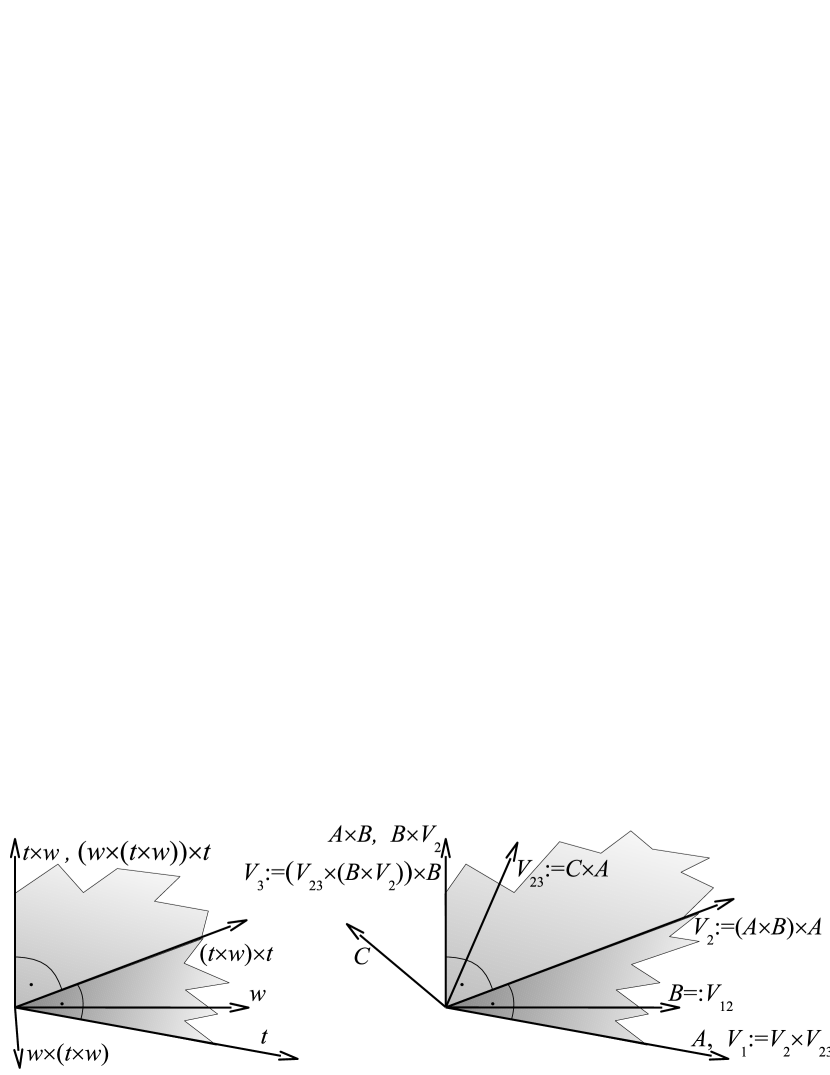
Figure 1: Illustrating the geometry of the terms considered a) in the reduction from $\operatorname{\textup{\sf XSAT}}^{0}_{\mathbb{P}^{2}(\mathbb{R})}$ to $\operatorname{\textup{\sf XSAT}}^{0}_{\mathbb{R}^{3}}$   and   b) in 9c.

Proof of 9c).

By construction, affine lines $A$ and $A\times B$ and $V_{2}$ are pairwise orthogonal; see Fig. 1b). Moreover $A\neq B$ because $A\times B$ a subterm of $V_{2}$ is defined by hypothesis. Since both $V_{2}$ and $V_{23}=C\times A$ are orthogonal to $A$, their projective cross product $V_{1}$ must coincide with $A$ whenever defined and in particular $V_{2}\neq V_{23}$; moreover $V_{2}$ and $V_{23}$ and $A\times B$ lie in a common plane. $B\times V_{2}$ as subterm of $V_{3}$ being defined requires $V_{2}\neq B$; yet these two and $A=V_{1}$ are orthogonal to $A\times B$ and thus lie in a common plane. In particular $B\times V_{2}=A\times B$. Finally, $V_{23}$ and $B\times V_{2}=A\times B$ both being orthogonal to $A$, their defined cross product as subterm of $V_{3}$ requires $V_{23}\neq B\times V_{2}$ and $V_{3}=B\times V_{2}=A\times B$. To summarize: $V_{1},V_{2},V_{3}$ are pairwise orthogonal; and $V_{1},V_{12},V_{2}$ are pairwise distinct yet all orthogonal to $V_{3}$; similarly $V_{2},V_{23},V_{3}$ are pairwise distinct yet all orthogonal to $V_{1}$. Now choose $0\neq\vec{v}_{1}\in V_{1}$ arbitrary and $\vec{v}_{2}\in V_{2}$ such that $V_{12}=\mathbb{F}(\vec{v}_{1}-\vec{v}_{2})$; finally choose $\vec{v}_{3}\in V_{3}$ such that $V_{23}=\mathbb{F}(\vec{v}_{2}-\vec{v}_{3})$. If these pairwise orthogonal vectors $\vec{v}_{1},\vec{v}_{2},\vec{v}_{3}$ happen to form a left-handed system, simply flip all their signs. ∎

4 Conclusion

We have identified a new problem complete (i.e. universal) for nondeterministic polynomial-time BSS machines, namely from exterior algebra: the satisfiability of a single equation built only by iterating cross products. This enriches algebraic complexity theory and emphasizes the importance of the Turing (!) complexity class $\operatorname{\textbf{{BP}}}(\textbf{{NP}}_{\!\mathbb{R}}^{0})$.

Moreover our proof yields a cross product equation $t^{\prime\prime\prime}_{X^{2}-2}(Y,A,B,C)=A$ solvable over $\mathbb{P}^{2}(\mathbb{R})$ but not over $\mathbb{P}^{2}(\mathbb{Q})$, the rational projective plane. In fact the decidability of $\operatorname{\textup{\sf XSAT}}^{0}_{\mathbb{P}^{2}(\mathbb{Q})}$ is equivalent to a long-standing open question [Poon09].

We wonder about the computational complexity of equations over the 7-dimensional cross product.

References

-
[BaMe13]
M. Baartse, K. Meer:
“The PCP Theorem for NP over the reals”,
pp.104–115 in Proc. 30th Symp. on Theoret. Aspects of Computer Science
(STACS’13), Dagstuhl LIPIcs vol.20.
10.4230/LIPIcs.STACS.2013.104
Full version to appear in Contemporary Mathematics, American Mathematical Society. - [BCSS98] L. Blum, F. Cucker, M. Shub, S. Smale: “Complexity and Real Computation”, Springer (1998).
- [BKOS97] M. de Berg, M. van Kreveld, M. Overmars, O. Schwarzkopf: “Computational Geometry, Algorithms and Applications”, Springer (1997).
- [BSS89] L. Blum, M. Shub, S. Smale: “On a Theory of Computation and Complexity over the Real Numbers: NP–completeness, Recursive Functions, and Universal Machines”, pp.1–46 in Bulletin of the American Mathematical Society (AMS Bulletin) vol.21 (1989). 10.1090/S0273-0979-1989-15750-9
- [Bürg00] P. Bürgisser: “Completeness and Reduction in Algebraic Complexity Theory”, Springer (2000)
- [BüSc09] P. Bürgisser, P. Scheiblechner: “On the Complexity of Counting Components of Algebraic Varieties”, pp.1114–1136 in Journal of Symbolic Computation vol.44:9 (2009). 10.1016/j.jsc.2008.02.009
- [Cann88] J. Canny: “Some Algebraic and Geometric Computations in PSPACE”, pp.460–467 in Proc. 20th annual ACM Symposium on Theory of Computing (SToC 1988). 10.1145/62212.62257
- [Cuck93] F. Cucker: “On the Complexity of Quantifier Elimination: the Structural Approach”, pp.400–408 in The Computer Journal vol.36:5 (1993). 10.1093/comjnl/36.5.400
- [CuRo92] F. Cucker, F. Rosselló: “On the Complexity of Some Problems for the Blum, Shub & Smale model”, pp.117–129 in Proc. LATIN’92, Springer LNCS vol.583. 10.1007/BFb0023823
- [GaJo79] M.R. Garey, D.S. Johnson: “Computers and Intractability: A Guide to the Theory of NP–completeness”, Freeman (1979).
- [Gius91] M. Giusti, J. Heintz: “Algorithmes – disons rapides – pour la décomposition d’une variété algébrique en composantes irréductibles et équidimensionnelles”, pp.169–193 in Effective Methods in Algebraic Geometry (Proceedings of MEGA’90), T. Mora and C. Traverso editors, Birkhäuser (1991).
- [Grig88] D.Y. Grigoriev: “Complexity of Deciding Tarski Algebra”, pp.65–108 in Journal of Symbolic Computation vol.5 (1988). 10.1016/S0747-7171(88)80006-3
- [HaSv96] H. Havlicek, K. Svozil: “Density Conditions for Quantum Propositions”, pp.5337–5341 in Journal of Mathematical Physics vol.37 (1996). 10.1063/1.531738
- [HeZi11] C. Herrmann, M. Ziegler: “Computational Complexity of Quantum Satisfiability”, pp.175–184 in Proc. 26th Annual IEEE Symposium on Logic in Computer Science (2011). 10.1109/LICS.2011.8
- [HRS90] J. Heintz, M.-F. Roy, P. Solernó: “Sur la complexité du principe de Tarski–Seidenberg”, pp.101–126 in Bull. Soc. Math. France vol.118 (1990).
- [Koir99] P. Koiran: “The Real Dimension Problem is –complete”, pp.227–238 in J. Complexity vol.15:2 (1999). 10.1006/jcom.1999.0502
- [Lece00] G. Lecerf: “Computing an Equidimensional Decomposition of an Algebraic Variety by means of Geometric Resolutions”, pp.209–216 in Proceedings of the 2000 International Symposium on Symbolic and Algebraic Computation (ISAAC), ACM. 10.1145/345542.345633
- [MeMi97] K. Meer, C. Michaux: “A Survey on Real Structural Complexity Theory”, pp.113–148 in Bulletin of the Belgian Mathematical Society vol.4 (1997).
- [MR95] R. Motvani, P. Raghavan: “Randomized Algorithms”, Cambridge University Press (1995).
- [Poon09] B. Poonen: “Characterizing Integers among Rational Numbers with a Universal-Existential Formula”, in American Journal of Mathematics vol.131:3 (2009).
- [Rene92] J. Renegar: “On the Computational Complexity and Geometry of the First-order Theory of the Reals”, pp.255–352 in Journal of Symbolic Computation vol.13:3 (1992). 10.1016/S0747-7171(10)80003-3 10.1016/S0747-7171(10)80004-5 10.1016/S0747-7171(10)80005-7
- [Rich99] J. Richter-Gebert: “The Universality Theorems for Oriented Matroids and Polytopes”, pp.269–292 in Contemporary Mathematics vol.223 (1999). 10.1090/conm/223/03144
- [Scha10] M. Schaefer: “Complexity of Some Geometric and Topological Problems”, pp.334–344 in Proc. 17th Int. Symp. on Graph Drawing, Springer LNCS vol.5849 (2010). 10.1007/978-3-642-11805-0_32
- [Shor91] P. Shor: “Stretchability of Pseudolines is NP–hard”, pp.531–554 in Applied Geometry and Discrete Mathematics — The Victor Klee Festschrift (P. Gritzmann and B. Sturmfels Edts), DIMACS Series in Discrete Mathematics and Theoretical Computer Science, vol.4 (1991). 10.1007/BF03025291
- [Smal98] S. Smale: “Mathematical Problems for the Next Century”, pp.7–15 in Math. Intelligencer vol.20:2 (1998).
- [Zhan92] X.-D. Zhang: “Complexity of Neural Network Learning in the Real Number Model”, pp.146–149 in Proc. Workshop on Physics and Computation (1992). 10.1109/PHYCMP.1992.615511