The initial mass function of star clusters that form in turbulent molecular clouds

Abstract

We simulate the formation and evolution of young star clusters using the combination of smoothed-particle hydrodynamical (SPH) simulations and direct $N$-body simulations. We start by performing SPH simulations of the giant molecular cloud with a turbulent velocity field, a mass of $4\times 10^{4}$ to $5\times 10^{6}M_{\odot}$, and a density between $\rho\sim 1.7\times 10^{3}$ and $170{\rm cm}^{-3}$. We continue the hydrodynamical simulations for a free-fall time scale ($t_{\rm ff}\simeq 0.83$ Myr and 2.5 Myr), and analyze the resulting structure of the collapsed cloud. We subsequently replace a density-selected subset of SPH particles with stars by adopting a local star-formation efficiency proportional to $\rho^{1/2}$. As a consequence, the local star formation efficiency exceeds 30 per cent, whereas globally only a few per cent of the gas is converted to stars. The stellar distribution by the time gas is converted to stars is very clumpy, with typically a dozen bound conglomerates that consist of 100 to $10^{4}$ stars. We continue to evolve the stars dynamically using the collisional $N$-body method, which accurately treats all pairwise interactions, stellar collisions and stellar evolution. We analyze the results of the $N$-body simulations when the stars have an age of 2 Myr and 10 Myr. During the dynamical simulations, massive clusters grow via hierarchical merging of smaller clusters. The shape of the cluster mass function that originates from an individual molecular cloud is consistent with a Schechter function with a power-law slope of $\beta=-1.73$ at 2 Myr and $\beta=-1.67$ at 10 Myr, which fits to observed cluster mass function of the Carina region. The superposition of mass functions have a power-law slope of $\ {\raise-2.15277pt\hbox{$\buildrel<\over{\sim}$}}\ -2$, which fits the observed mass function of star clusters in the Milky Way, M31 and M83. We further find that the mass of the most massive cluster formed in a single molecular cloud with a mass of $M_{\rm g}$ scales with $6.1M_{\rm g}^{0.51}$ which also agrees with recent observation of the GMC and young clusters in M51.

1 Introduction

Observed star forming regions show filamentary or spumous structure, which appears to be a natural consequence of the star formation process (André et al., 2010). Star forming regions are thought to be the results of the gravitational collapse of giant molecular clouds (McKee & Ostriker, 2007, and references therein). Once the stars have formed they start to develop a wind, and then the first supernovae explosions occur a few million years later. These outflows cause the residual gas to be blown away. The stellar distribution as a consequence will be super-virial after all the gas is lost, but virial equilibrium is quickly re-established, after which the cluster will have lost some stars and the remaining bound stars eventually form a spherical and centrally concentrated distribution. There are numerous observed examples of such young clusters that are about to emerge from their parental molecular cloud (Lada & Lada, 2003, and references therein).

The initial collapse of the molecular cloud is also driven by (magneto)hydrodynamical processes, radiation, and chemical reactions, in contrast to the purely dynamical evolution of gas-deprived clusters. These processes have been studied extensively from an observational point of view (Keto & Wood, 2006; Zinnecker & Yorke, 2007; Zapata et al., 2008) and numerically (Bonnell et al., 2008; Peters et al., 2010; Bate, 2012; Krumholz, 2012; Krumholz et al., 2012b; Krumholz & Thompson, 2012; Federrath & Klessen, 2012). During the transition phase from a gas dominated cluster to a purely stellar cluster, the spectrum of physical processes broadens dramatically and includes hydrodynamics, gravity, nuclear fusion and radiation processes. It is only at the later, gas deprived state, that dynamical process start to dominate the evolution of the stellar system.

Most numerical studies aim at one of these extremes, either the star formation process (e.g., Bonnell et al., 2003, 2008) or the gas-deprived evolution of the star cluster starting from artificial fractal initial conditions (e.g., Parker et al., 2014). In some studies the final conditions of the former are used as initial conditions for the latter (Moeckel & Bate, 2010; Moeckel et al., 2012). In Moeckel & Bate (2010) and Moeckel et al. (2012) the problem is addressed in some discrete steps. They start by performing a hydro-dynamical simulation including sink-particles to follow the growth in mass of two accreting point-masses which represent proto-stellar objects. After about one free-fall time of the molecular cloud they instantaneously remove all the residual gas and continue the simulation using a direct $N$-body code to study the dynamical evolution of the gas-deprived stellar system.

Although removing the gas instantaneously is an extreme measure, their approach appears to work well. The densest parts of their stellar distributions are relatively small 0.1–0.2 pc and already rather deprived of residual gas (Kruijssen et al., 2012; Moeckel et al., 2012). The relatively small and dense stellar clumps therefore survive even under their rather extreme assumption of instantaneous gas expulsion.

We aim to acquire a better understanding of the formation process of star clusters, using a method similar to the one used in Moeckel & Bate (2010). We decide to adopt a lower resolution to avoid using sink particles. As in Moeckel & Bate (2010), we start by performing a hydrodynamical simulation for about a free-fall time, after which we analyze the results and generate stars. The residual gas is removed instantaneously, and we continue the simulation by means of direct $N$-body integration. Instead of using sink-particles, we convolve gas particles to stars adopting a simple star-formation efficiency (SFE) that depends on the local free-fall time. This procedure is considerably easier to implement and requires much less computer time, and therefore we can treat clusters with a mass of $>10^{4}M_{\odot}$, that was not possible in previous simulations. Such a method also allows us to have more control over the star formation process, and it makes the interpretation of the result more transparent.

In our experiments, we are particularly interested in the earliest dynamical evolution of the clusters, as it formed in a collapsed molecular cloud after the gas expulsion. We study this dynamical evolution up to about 2 Myr for clusters with a mass of $\sim 10^{4}\,M_{\odot}$. We refer to these clusters as young massive clusters. Our study is motivated by the recent finding of the accretion of a smaller stellar clump in R136 (Sabbi et al., 2012), but we are also intrigued by the formation processes of Westerlund 1, Westerlund 2 and NGC 3603, because recent studies using $N$-body simulations suggest that they formed via mergers of smaller sub-clusters (Fujii et al., 2012).

2 Numerical methods

In our simulations we combine a smoothed particles hydrodynamics (SPH) code with a direct $N$-body code. The method consists of three steps:

1. Perform an SPH simulation of a turbulent molecular cloud for an initial free-fall time scale.

2. Convert gas particles to stellar particles assuming a star formation efficiency (SFE), which depends on the local gas density, and remove the residual gas (SPH particles).

3. Turn on the direct $N$-body simulation for integrating the equations of motion of the stellar particles.

The initial conditions for SPH simulations are taken from an isothermal homogeneous gas sphere with a turbulent velocity field (Bonnell et al., 2003) with a spectral index of $k=-3$. The size and total mass for our standard model are 10 pc and $4\times 10^{5}M_{\odot}$, respectively. The mean gas density is then $\sim 100M_{\odot}{\rm pc}^{-3}$($\sim 1700\,{\rm cm}^{-3}$ assuming that the mean weight per particle is $2.33m_{\rm H}$) and the free-fall time $t_{\rm ff}=0.83$ Myr.

2.1 The hydrodynamical collapse of the molecular cloud

We initialize the gas cloud by giving it zero total energy (potential plus kinetic). We perform additional simulations with a mean gas density of $\sim 10M_{\odot}{\rm pc}^{-3}$ ($\sim 170\,{\rm cm}^{-3}$) by increasing the overall dimension of the system and adopting a total mass of $4\times 10^{4}$–$2\times 10^{6}M_{\odot}$. With a mean gas density of $\sim 10M_{\odot}{\rm pc}^{-3}$, $t_{\rm ff}=2.5$ Myr. We adopt a gas temperature of 30K. We summarize the initial conditions of the simulations in Table 1. For each initial condition, we perform 1–3 runs with different random seeds for the generation of the turbulence in order to see the run-to-run variation. The number of random seeds are indicated as ’s’ in the table.

For our SPH simulations, we adopt $1M_{\odot}$ per particle. The SPH softening length ($h$) is chosen such that $\rho h^{3}=mN_{\rm nb}$ (Springel & Hernquist, 2002), where $\rho$ is the density, $m$ and the particle mass, and $N$ is the target number of neighbor particles. We adopt $N_{\rm nb}=64$, with which the mass resolution is $\sim 100M_{\odot}$. With this setup, the minimum scale we can resolve the Jeans instability is $h=1.7$ pc. These mass and size are comparable to the typical ($\sim 1$ pc) size of embedded clusters (Lada & Lada, 2003). Our SPH simulations therefore cannot resolve the formation of individual stars. The gravitational softening length is taken to be constant (approximately the smallest softening length encountered in the simulation) $\epsilon_{\rm grav}=0.1$ pc for the gas particles in order to improve energy and momentum conservation. The resolution of our simulations are lower than recent simulations which aim at simulating star formation in turbulent molecular clouds (Bonnell et al., 2011; Bate, 2012). We motivate this relatively low resolution by our aim at reproducing the clumpy structure of star forming regions, rather than the microscopic details of the star formation process. Of course, ideally we would like to resolve also the latter, but this is currently unpractical, at least, and we think that our approach is reasonable and a considerable advance over adopting a simple virialized Plummer sphere (Plummer, 1911) or King model (King, 1966) to generate the initial realization for the gravitational $N$-body simulations.

The generation of the initial conditions and the SPH simulations are performed with the Astronomical Multipurpose Software Environment (AMUSE) (Portegies Zwart et al., 2013; Pelupessy et al., 2013). AMUSE is a follow-up of the earlier MUSE environment Portegies Zwart et al. (2009), which was intended to be a general purpose framework for performing large scale astronomical simulations. In the AMUSE framework we adopted the Python programming language to encapsulate the fundamental physics solvers, which are written in high-performance compiled computer code. The flexibility of AMUSE makes it possible to perform simulations with one implementation of the numerical solver, and then repeat the same calculation with a different solver by changing one line in the AMUSE-python script.

As the engine for performing the hydrodynamical simulation we adopted the SPH code Fi (Hernquist & Katz, 1989; Gerritsen & Icke, 1997; Pelupessy et al., 2004; Pelupessy, 2005). Within Fi the internal time step is controlled internally, but we constrain this timestep from within the framework to 0.025 Myr.

Figure 1: Gas surface density at an age of $0.9t_{\rm ff}$ for model m400k-d100-30K.

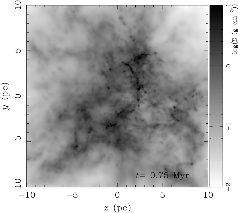
We stop the hydrodynamical simulation at $0.9t_{\rm ff}$. By this time the volume density reaches $10^{7-8}{\rm cm}^{-3}$ ($10^{6-7}M_{\odot}\mathrm{pc}^{-3}$) and the surface density reaches a value of $10\mathrm{g}\,\mathrm{cm}^{-2}$ ($10^{5}M_{\odot}{\rm pc}^{-2}$). In Figure 1 we present an example of the gas density distribution at the moment we stop the hydrodynamical calculations.

Table 1: Models for hydrodynamical simulations (’s’ indicates the random seeds for the turbulence).

Model	Total mass	$N$ of particles	Radius	Density	Thermal Energy	Temperature
	$M_{\rm g}(M_{\odot})$	$N_{\rm g}$	$r_{\rm g}$(pc)	$\rho_{\rm g}({\rm cm}^{-3})$	$E_{\rm t}/E_{\rm k}$	$T$ (K)
m2M-d10-s18-30K	$2\times 10^{6}$	$2\times 10^{6}$	35.9	170	$1.1\times 10^{-3}$	30
m1M-d100-s7-30K	$1\times 10^{6}$	$1\times 10^{6}$	13.4	$1.7\times 10^{3}$	$8.4\times 10^{-4}$	30
m1M-d100-s12-30K	$1\times 10^{6}$	$1\times 10^{6}$	13.4	$1.7\times 10^{3}$	$8.4\times 10^{-4}$	30
m1M-d100-s10-30K	$1\times 10^{6}$	$1\times 10^{6}$	13.4	$1.7\times 10^{3}$	$8.4\times 10^{-4}$	30
m1M-d10-s3-30K	$1\times 10^{6}$	$1\times 10^{6}$	28.5	170	$1.7\times 10^{-3}$	30
m1M-d10-s4-30K	$1\times 10^{6}$	$1\times 10^{6}$	28.5	170	$1.7\times 10^{-3}$	30
m400k-d100-s1-30K	$4\times 10^{5}$	$4\times 10^{5}$	10.0	$1.7\times 10^{3}$	$1.6\times 10^{-3}$	30
m400k-d100-s5-30K	$4\times 10^{5}$	$4\times 10^{5}$	10.0	$1.7\times 10^{3}$	$1.6\times 10^{-3}$	30
m400k-d100-s11-30K	$4\times 10^{5}$	$4\times 10^{5}$	10.0	$1.7\times 10^{3}$	$1.6\times 10^{-3}$	30
m400k-d10-s8-30K	$4\times 10^{5}$	$4\times 10^{5}$	21.0	170	$3.3\times 10^{-3}$	30
m400k-d10-s9-30K	$4\times 10^{5}$	$4\times 10^{5}$	21.0	170	$3.3\times 10^{-3}$	30
m100k-d100-s2-30K	$1\times 10^{5}$	$1\times 10^{5}$	6.2	$1.7\times 10^{3}$	$3.9\times 10^{-3}$	30
m100k-d100-s6-30K	$1\times 10^{5}$	$1\times 10^{5}$	6.2	$1.7\times 10^{3}$	$3.9\times 10^{-3}$	30
m100k-d100-s13-30K	$1\times 10^{5}$	$1\times 10^{5}$	6.2	$1.7\times 10^{3}$	$3.9\times 10^{-3}$	30
m40k-d100-s20-30K	$4.1\times 10^{4}$	$4.1\times 10^{4}$	4.6	$1.7\times 10^{3}$	0.0071	30
m40k-d100-s21-30K	$4.1\times 10^{4}$	$4.1\times 10^{4}$	4.6	$1.7\times 10^{3}$	0.0071	30
m40k-d100-s22-30K	$4.1\times 10^{4}$	$4.1\times 10^{4}$	4.6	$1.7\times 10^{3}$	0.0071	30

2.2 Forming the stars

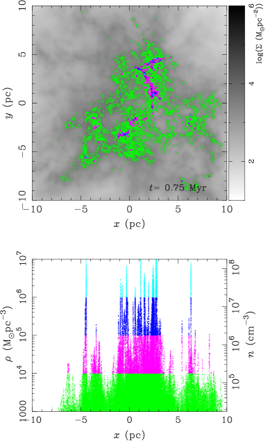
We continue by analyzing the resulting density distribution of the collapsed molecular gas cloud. In Figure 2 we present a projected image of the density distribution of the gas at an age of 0.75 Myr ($\sim 0.9t_{\rm ff}$) after the start of the hydrodynamical simulation. The densest regions reached $\sim 10^{6}M_{\odot}{\rm pc}^{-3}$, which is consistent to the results from earlier SPH simulations that included star formations through sink particles (Moeckel & Bate, 2010).

Figure 2: Gas surface density at $0.9t_{\rm ff}$ for model m400k-d100-30K (top panel in gray scale). Colors indicate dense region; cyan, blue, magenta, green indicates regions with the volume density of $>10^{6}$, $10^{5-6}$, $10^{4-5}$, and $10^{3-4}M_{\odot}$pc^-3, respectively. Gas volume density distribution projected on $x$-axis (bottom). Colors are the same as in top panel.

The conversion of the SPH particles to stars was realized by adopting a local star formation efficiency, $\epsilon_{\rm loc}$, which we calculate using

$$\epsilon_{\rm loc} = \alpha_{\rm sfe}\sqrt{\frac{\rho}{10^{2}(M_{\odot}{\rm pc}^{-3})}}$$ (1)

$$= \alpha_{\rm sfe}\sqrt{\frac{\rho}{1.7\times 10^{3}({\rm cm}^{-3})}}.$$ (2)

Here $\rho$ is the local volume density, which is measured at the location of each individual SPH particle in the simulation. The coefficient, $\alpha_{\rm sfe}$, controls the star formation efficiency and is a free parameter in our simulations. With this prescription, the local SFE correlates with the instantaneous free-fall time of the gas via the square-root of the gas density. This assumption is motivated by recent result that indicate that the star formation rate scales with the free-fall time (Krumholz et al., 2012a). We adopted $\alpha_{\rm sfe}=0.02$ for the models with $\rho_{\rm g}=100M_{\odot}{\rm pc}^{-3}$, which is similar to what was obtained by Krumholz et al. (2012a). We chose a higher value of $\alpha_{\rm sfe}=0.04$ for $\rho_{\rm g}=170{\rm cm}^{-3}$, because in these cases the time for a part of the system to evolve from the moment when it reaches $1700{\rm cm}^{-3}$ to the end of the hydrodynamical simulation is twice as long as the free-fall time of the models with $1700{\rm cm}^{-3}$.

Figure 3: The initial spatial distribution of the stars for the $N$-body simulation.

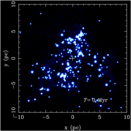
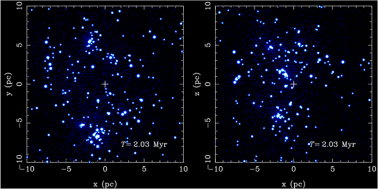
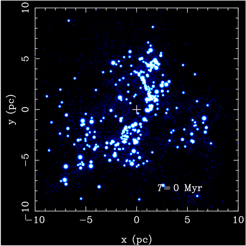
We replace the densest SPH particles with stellar particles by adopting the local star formation efficiency of equation (2). This resulted in the star formation efficiency in the dense regions ($\rho\geq 1.7\times 10^{4}{\rm cm}^{-3}$ i.e., $10^{3}M_{\odot}{\rm pc}^{-3}$), $\epsilon_{\rm d}$, of 20–30% which is consistent with the observed star formation efficiency (Lada & Lada, 2003). The residual gas is assumed to be ejected from the system. In Figure 3 we present the stellar distribution that is obtained from the hydrodynamical simulation after the SPH particles have been converted to stars and the residual gas is removed.

The positions and velocities of the stars are identical to those of the SPH particles from which they formed. The mass of a star was selected randomly from the Salpeter (1955) mass function between a minimum and maximum mass of 0.3 $M_{\odot}$ and 100 $M_{\odot}$. The mean mass of this distribution turns out to be $1M_{\odot}$. As a consequence, this method does not conserve mass locally, but globally mass is conserved. After removing all SPH particles, the residual stellar system was super-virial with a virial ratio $Q_{\rm vir}>1$. We did not generate any primordial binaries in the initial conditions because during our integration time ($\ {\raise-2.15277pt\hbox{$\buildrel<\over{\sim}$}}\ 10$Myr) hard binaries which are tight enough to affect on the dynamical evolution of the host clusters interact only very rarely with the surrounding stars due to their small separations (Fujii & Portegies Zwart, 2011).

The global star formation efficiency, $\epsilon$, for the entire molecular structure turned out to be a few per cent. This fraction is a result of the simulations and the adopted local star formation efficiency. In Table 2 we give the values for $\epsilon$ and $\epsilon_{\rm d}$ obtained from our simulations.

Table 2: Models for $N$-body simulations

Model	Total mass	$N$ of particles	Virial ratio	SFE (Global)	SFE (Dense)
	$M_{\rm s}(M_{\odot})$	$N_{\rm s}$	$Q_{\rm vir}$	$\epsilon$	$\epsilon_{\rm d}$
m2M-d10-s18-30K	$1.0\times 10^{5}$	99546	3.9	0.050	0.39
m1M-d100-s7-30K	$1.1\times 10^{5}$	109952	6.1	0.11	0.26
m1M-d100-s12-30K	$9.4\times 10^{4}$	94464	2.2	0.096	0.23
m1M-d10-s3-30K	$7.8\times 10^{4}$	78201	0.66	0.079	0.54
m1M-d10-s4-30K	$5.7\times 10^{4}$	56681	2.2	0.058	0.41
m400k-d100-s1-30K	$3.0\times 10^{4}$	30487	2.4	0.074	0.21
m400k-d100-s5-30K	$2.4\times 10^{4}$	24211	4.8	0.059	0.16
m400k-d100-s11-30K	$4.0\times 10^{4}$	39933	1.5	0.074	0.26
m400k-d10-s8-30K	$1.9\times 10^{4}$	19236	2.8	0.047	0.39
m400k-d10-s9-30K	$2.0\times 10^{4}$	19672	2.6	0.047	0.36
m100k-d100-s2-30K	$1.3\times 10^{4}$	12833	0.58	0.13	0.34
m100k-d100-s6-30K	$4.6\times 10^{3}$	4572	7.8	0.045	0.14
m100k-d100-s13-30K	$8.0\times 10^{3}$	7987	1.9	0.079	0.22
m40k-d100-s20-30K	$2.9\times 10^{3}$	2866	1.7	0.079	0.21
m40k-d100-s21-30K	$3.2\times 10^{3}$	3175	1.9	0.077	0.21
m40k-d100-s22-30K	$2.1\times 10^{3}$	2073	2.0	0.051	0.16

2.3 The dynamical evolution of the cluster

We now use the stellar masses, positions, and velocities as initial realizations for our $N$-body calculations in which we study the dynamical evolution of the stellar system. For convenience we associate the moment at which we start the $N$-body simulations with $t=0$ Myr. The forces between each pair of stars is calculated directly, and the numerical integration of the equations of motion was performed using the sixth-order Hermite scheme (Nitadori & Makino, 2008). The $N$-body code runs without softening and with a time step parameters $\eta=0.1$–0.3. The energy error was less than 0.1% for all simulations. It is small enough for obtaining a scientifically interpretable result in such $N$-body simulations (Portegies Zwart & Boekholt, 2014).

If two stars approach each other closer than the sum of their radii, we resolve the collision by summing the mass and conserving the angular momentum. The stellar radius was calculated using the description in (Hurley et al., 2000; Toonen et al., 2012) and for stars $>100M_{\odot}$ we extrapolated the results (see Fujii et al., 2009, 2012, for the details). We only adopted very simple stellar evolution prescription in which a star turns into a black hole directly after the main sequence (Hurley et al., 2000). The supernovae were assumed to be symmetric and therefore no natal kick was delivered to the compact remnant. By the end of the simulations (10 Myr), stars with a mass of $\ {\raise-2.15277pt\hbox{$\buildrel>\over{\sim}$}}\ 20M_{\odot}$ reaches the end of their main-sequence life-time and evolve to black holes.

Table 3: The results of simulations at $t=2$Myr. $M_{\rm s,cl}/M_{\rm s}$ is the stellar mass fraction which belongs to clusters. $M_{\rm c,max}$ is the mass of the most massive clusters formed in the simulations. $N_{\rm c}$ is the number of clusters. $\beta_{1}$ is the power of the fitted cluster mass function adopting the value of $M_{\rm c,max}$ obtained from the simulations. $\beta_{2}$ and $A$ are the power and the factor of the fitted cluster mass function (equation (5)) but with $M_{\rm c,max}=0.20M_{\rm g}^{0.76}$. The fitting results exist only for models with $N_{\rm c}>4$. Averaging the results, we obtain $\beta_{1}=-1.71\pm 0.18$, $\beta_{2}=-1.73\pm 0.17$, and $A=0.64\pm 0.29$.

Model	$M_{\rm s,cl}/M_{\rm s}$	$M_{\rm c,max}(M_{\odot})$	$N_{\rm c}$	$\beta_{1}$	$\beta_{2}$	$A$
m2M-d10-s18-30K	0.31	$3.1\times 10^{4}$	61	$-1.68\pm 0.02$	$-1.60\pm 0.08$	$0.93\pm 0.15$
m1M-d100-s7-30K	0.43	$9.5\times 10^{3}$	51	$-1.65\pm 0.02$	$-1.64\pm 0.02$	$1.13\pm 0.10$
m1M-d100-s12-30K	0.40	$8.9\times 10^{3}$	50	$-1.74\pm 0.02$	$-1.73\pm 0.02$	$0.72\pm 0.05$
m1M-d10-s3-30K	0.42	$2.4\times 10^{4}$	30	$-2.16\pm 0.04$	$-2.14\pm 0.04$	$0.09\pm 0.01$
m1M-d10-s4-30K	0.33	$2.5\times 10^{3}$	45	$-1.93\pm 0.04$	$-2.00\pm 0.03$	$0.26\pm 0.03$
m400k-d100-s1-30K	0.33	$3.0\times 10^{3}$	15	$-1.53\pm 0.05$	$-1.55\pm 0.05$	$0.73\pm 0.12$
m400k-d100-s5-30K	0.40	$2.7\times 10^{3}$	16	$-1.59\pm 0.07$	$-1.62\pm 0.07$	$0.82\pm 0.16$
m400k-d100-s11-30K	0.37	$7.4\times 10^{3}$	14	$-1.64\pm 0.04$	$-1.58\pm 0.04$	$0.78\pm 0.11$
m400k-d10-s8-30K	0.38	$1.4\times 10^{3}$	18	$-1.63\pm 0.05$	$-1.71\pm 0.04$	$0.50\pm 0.06$
m400k-d10-s9-30K	0.36	$2.1\times 10^{3}$	17	$-1.71\pm 0.06$	$-1.75\pm 0.06$	$0.46\pm 0.08$
m100k-d100-s2-30K	0.41	$5.0\times 10^{3}$	4	-	-	-
m100k-d100-s6-30K	0.35	$3.9\times 10^{2}$	7	$-1.46\pm 0.20$	$-1.81\pm 0.22$	$0.38\pm 0.17$
m100k-d100-s13-30K	0.45	$8.5\times 10^{2}$	11	$-1.51\pm 0.08$	$-1.60\pm 0.08$	$0.08\pm 0.16$
m40k-d100-s20-30K	0.35	$4.9\times 10^{2}$	4	-	-	-
m40k-d100-s21-30K	0.28	$3.2\times 10^{2}$	2	-	-	-
m40k-d100-s22-30K	0.28	$8.5\times 10^{2}$	2	-	-	-

Table 4: The results of simulations at 10Myr. Averaging the results, we obtain $\beta_{1}=-1.53\pm 0.16$, $\beta_{2}=-1.67\pm 0.30$, and $A=0.63\pm 0.30$. Here, we assume $M_{\rm c,max}=0.20M_{\rm g}^{0.76}$.

Model	$M_{\rm c,max}(M_{\odot})$	$N_{\rm c}$	$\beta_{1}$	$\beta_{2}$	$A$
m400k-d100-s1-30K	$5.3\times 10^{3}$	9	$-1.41\pm 0.05$	$-1.35\pm 0.06$	$0.84\pm 0.16$
m400k-d100-s5-30K	$2.3\times 10^{3}$	14	$-1.60\pm 0.05$	$-1.58\pm 0.04$	$0.83\pm 0.10$
m100k-d100-s2-30K	$5.2\times 10^{3}$	4	-	-	-
m100k-d100-s6-30K	$4.6\times 10^{2}$	5	$-1.75\pm 0.08$	$-2.07\pm 0.08$	$0.20\pm 0.03$

3 Cluster Mass Function

3.1 Cluster Finding

At an age of 2 Myr and at 10 Myr, we interrupt the simulations to study the clumps in the stellar distribution. We identify these clumps as star clusters.

These clusters are detected using the HOP (Eisenstein & Hut, 1998) clump finding algorithm (which is also incorporated in the AMUSE framework). The outer cut-off density (somewhat related to the density of an individual clump) was set to $\rho_{\rm out}=4.5M_{\rm s}/(4\pi r_{\rm h}^{3})$, which is three times the half-mass density of the entire system. Other parameters in HOP are the number of particles to calculate the local density, for which we adopted $N_{\rm dense}=64$, the number of particles for neighbor search ($N_{\rm hop}=64$) and the number of particles of neighbors to determine for two groups to merge ($N_{\rm merge}=4$). Because star clusters have a relatively high density contrasts compared to dark matter halos, to which the method is applied with the default parameters, we adopted $8\rho_{\rm out}$ for the saddle density threshold and $10\rho_{\rm out}$ for the peak density threshold. We do not include clusters with fewer than 64 stars in our analysis, because both the SPH simulations and the clump finding method used for analysis cannot resolve them. Such small clusters hardly ever exceed $100M_{\odot}$, which is consistend with the generally adopted minimum mass for a star cluster, regardless the arbitraryness of this choise. We adopted these parameter because HOP was most successful in detecting all the clusters, but verified that changing the parameters does not influence our results qualitatively. The clumps detected are not necessarily bound, but we detected the members based on geometry. This might not be what a theorist normally would identify as a cluster, but from an observational point of view it is often hard to separate out the unbound stars from the bound stars. With the adopted method we mimic an observational identification criterion.

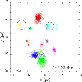
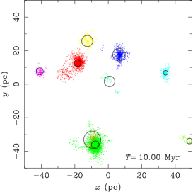
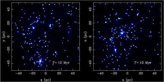
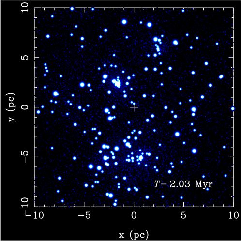
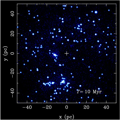
After identifying all clusters, we determine their total mass and half-mass radius. In Figure 4 we present two examples at 2 Myr and at 10 Myr of the clusters identified using this procedure.

Figure 4: Projected snapshots of model m400k-d100-30K at 2 Myr (top) and at 10 Myr (bottom). The results of the clump finding algorithm are presented in the left-most two panels. Each clump is presented in a single color, and the black circles show the respective half-mass radii of the clumps. Overlaying circles are separated in the third dimension. To the right we present two projections ($x$-$y$ in the middle and $y$-$z$ in the right) of all the stars in the simulation.

3.2 The Star-Cluster Mass Function

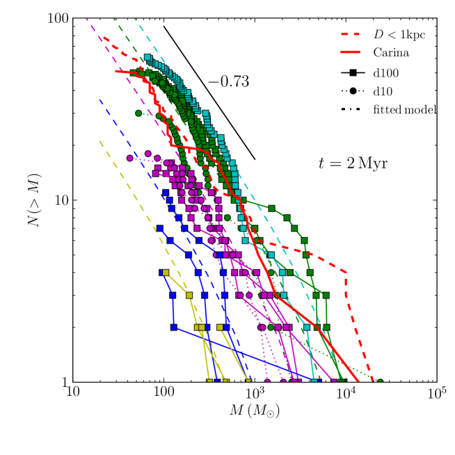
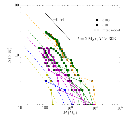
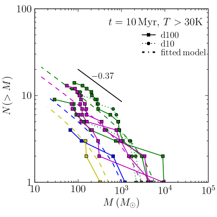
For each simulation we can now construct a mass function (MF) of star clusters. In Figure 5 we present the cumulative mass distribution for star clusters in our simulations. The offset scatter among the models is large, but the power of the MF is similar, irrespective of the model. We compare the obtained MFs with the Schechter function:

$$\phi(M)\equiv\frac{dN}{dM}\propto M^{\beta}\exp\left(-\frac{M}{M_{\rm cut}}\right).$$ (3)

Here $M$ is the mass of clusters and $M_{\rm cut}$ is the cut-off mass. Integration of equation (3) results in the cumulative MF, which has the form

$$N(>M)\propto M^{\beta+1}\exp\left(-\frac{M}{M_{\rm cut}}\right).$$ (4)

We use equation (4) to fit (using least mean squares) the mass distribution of the clusters we obtained in each of our simulations. The average of the best fit parameter for all models together is $\beta=-1.55\pm 0.41$ for the slope of the mass function. The uncertainty in the fitting procedure for detarmining $M_{\rm cut}$ is very large.

Figure 5: Cumulative cluster mass function obtained from the simulations with a temperature of 30K when the stars had an age of 2 Myr. The colors represent different masses of initial molecular clouds: cyan, green, magenta, blue, and yellow indicate $M_{\rm g}$ of $2\times 10^{6},10^{6},4\times 10^{5},10^{5}$ and $4\times 10^{4}M_{\odot}$, respectively. The dashed curves give the fitted MF (see equation (5)). We adopt $A=0.64$, $\beta=-1.73$, and $M_{\rm c,max}=0.20M_{\rm g}^{0.76}$. The red dashed curve is the mass function of the MW young clusters ($<3$ Myr) within 1 kpc from the Sun (indicated by $D<1$kpc). The data is from (Lada & Lada, 2003; Piskunov et al., 2008; Portegies Zwart et al., 2010). We here assumed that all the (embedded) clusters in Lada & Lada (2003) are younger than 3 Myr. Red thick curve is the cluster mass function of the Carina region (Feigelson et al., 2011).

Even though we were unable to determine a reliable value for $M_{\rm cut}$, we can use the mass of the most massive cluster ($M_{\rm c,max}$) as $M_{\rm cut}$. Scaling equation (4) by assuming that $M_{\rm cut}=M_{\rm c,max}$ , the cumulative mass function becomes

$$N(>M)=\frac{AM^{\beta+1}\exp\left(-\frac{M}{M_{\rm c,max}}\right)}{M_{\rm c,max}^{\beta+1}\exp\left(-1\right)}.$$ (5)

Here $A$ is a factor and we scaled in such a way that $N=A$ for $M=M_{\rm c,max}$. Fitting this function to the cluster mass functions results in $\beta=-1.71\pm 0.18$. In Table 3 we give for each model the maximum cluster mass and best fit parameters.

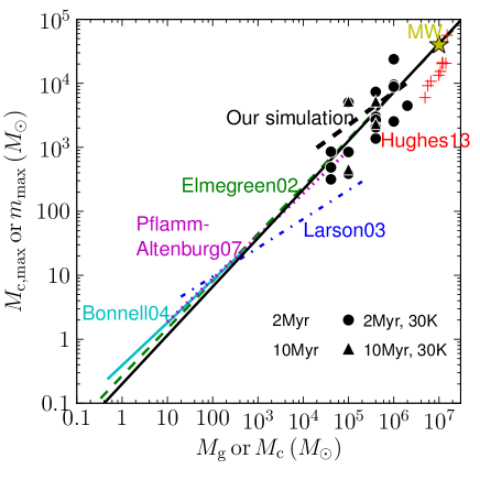
There appears to be a clear relation between the most massive cluster ($M_{\rm c,max}$) and the initial total mass in gas ($M_{\rm g}$), which we fitted using least squares to the form $M_{\rm c,max}=6.3M_{\rm g}^{0.51}$. In Figure 6 we over plot the results of the simulations with the fitted function (black thick dashed line). To compare with observations, we over-plot recent results of the mass of the most massive GMCs and star clusters in different regions in M51 (Hughes et al., 2013). If we consider that the most massive GMC forms the most massive star cluster, this observational result is directly comparable to our results. Interestingly, this relation is also quite consistent with the relation between the mass of the most massive star ($m_{\rm max}$) and its host cluster ($M_{\rm c}$) found in observations (Larson, 2003; Pflamm-Altenburg et al., 2007), simulations (Bonnell et al., 2004), and theoretical models (Elmegreen, 2002). We make the connection between this relation and stellar scales by adopting a minimum stellar mass (brown dwarf) of $0.01M_{\odot}$ which with a 50% SFE must have formed from a gas cloud with a mass of $0.02M_{\odot}$. When we include this point as a boundary condition in the fitting procedure, we obtain $M_{\rm c,max}=0.20M_{\rm g}^{0.76}$ as a best fit to the data (including this artificial point). This result does not strongly depend on the value of the artificial point. If we adopt the stellar mass of $0.5M_{\odot}$ and the parental gas mass of $2.15M_{\odot}$, which is obtained from the relation between the gas mass and the stellar mass in Bonnell et al. (2004), we obtain $M_{\rm c,max}=0.28M_{\rm g}^{0.74}$. Using this empirical relation we estimate the mass of the most massive star cluster in the Milky Way (MW) that formed from the most massive GMC. According to our analysis, the most massive GMC in the Milky Way is about $\sim 10^{7}M_{\odot}$ (Murray, 2011), and it could form a star cluster with a mass of $\sim 3\times 10^{4}M_{\odot}$. This estimate for the most massive star cluster is consistent with that of Westerlund 1 ($3\times 10^{4}M_{\odot}$), RSGC01, 02, 03 (3–$4\times 10^{4}M_{\odot}$), and Arches ($2\times 10^{4}M_{\odot}$ Portegies Zwart et al., 2010). For clarity, we present in Figure 6 the observed MW cluster and GMC.

When we adopt the relation $M_{\rm cut}=M_{\rm max,c}=0.20M_{\rm g}^{0.76}$, equation (5) still fits satisfactorily to the simulations, which then results in $\beta=-1.73\pm 0.17$ and $A=0.64\pm 0.29$. And adopting $M_{\rm cut}=M_{\rm max,c}=6.3M_{\rm g}^{0.51}$ results in $\beta=-1.75\pm 0.17$ and $A=0.56\pm 0.32$. The values of $A$ and $\beta$ for each model are presented in Table 3. We ignore models in with fewer than 5 clumps were detected, because the resulting statistics becomes unreliable. This fit is presented as the dashed lines in Figures 5 (indicated with “fitted model”). This relation is slightly shallower than the observed power-law ($\beta\simeq-2$) mass function for massive clusters in Galactic disk and starburst galaxies (Portegies Zwart et al., 2010, and references therein). We discuss this in section 4. Note that the run-to-run variation in our simulations is relatively large. The mass of the most massive cluster, for example, varies by about an order of magnitude. Model m40k-d100-30K models are an extreme case (see blue squares in Figure 5).

We also compared our simulation results with the observed young-cluster mass-function in the MW (data from Lada & Lada, 2003; Piskunov et al., 2008; Portegies Zwart et al., 2010), and in the Carina region (data from Feigelson et al., 2011), which fits $\beta=-1.66\pm 0.01$. This curve is presented in Figure 5 as the solid red curve. The observed mass function is consistent with our models for $M_{\rm g}\simeq 10^{6}M_{\odot}$.

In our simulations the star formation efficiency and consequently the maximum mass of a star clusters, depends slightly on the initial density of the molecular cloud. The total stellar mass correlates with $\sqrt{\rho_{\rm g}}$, because we assumed the local star formation efficiency to depend on the local gas density. As a consequence the star formation efficiency is highest in the densest regions.

Figure 6: The relation between the mass of the most massive cluster ($M_{\rm c,max}$) and the total mass of the molecular cloud ($M_{\rm g}$) or between the mass of the most massive star ($m_{\rm max}$) and the total mass of its host cluster ($M_{\rm c}$). Black dots and triangles indicate the results of our simulations with 30K for $t=$2 Myr and 10 Myr, respectively. Thick dashed line indicates the fitted function to our result ($M_{\rm c,max}=6.3M_{\rm g}^{0.51}$), and thick full line is also fitted but forced to at $m_{\rm s}=0.01M_{\odot}$ at $M_{\rm g}=0.02M_{\odot}$ ($M_{\rm c,max}=0.20M_{\rm g}^{0.76}$). Red pluses indicate the observed relation between the mass of the most massive GMCs and clusters in different environments in M51 (Hughes et al., 2013). Star indicates the most massive cluster and GMC in the MW. The color thin dashed, dash-dotted, full, and dotted lines give the relation between the mass of the most massive star as a function of its host cluster mass; $m_{\rm s,max}=0.27M_{\rm c}^{0.74}$ (Elmegreen, 2002), $m_{\rm s,max}=1.2M_{\rm c}^{0.45}$ (Larson, 2003), $m_{\rm s,max}=0.3M_{\rm c}^{2/3}$ (Bonnell et al., 2004), and $m_{\rm s,max}=0.4M_{\rm c}^{0.67}$(Pflamm-Altenburg et al., 2007), respectively (see also Weidner et al. (2010)). The length of each line is proportional to the mass range from which the relation is obtained.

3.3 The Secular Evolution of the Cluster Mass Function due to Mergers

In our simulations, clusters form hierarchically; more massive clusters form from repeated mergers. Gravitationally bound small stellar clumps form quickly after the residual gas is removed. Each clump corresponds to one of the density peaks in the parental gas distribution (see Figure 2). In the first few Myr, the clumps grow in mass primarily by accreting smaller structures, but by an age of about 2 Myr, the cluster population has almost established itself. At that moment $\sim$ 30% of the stars belong to a cluster (see $M_{\rm s,cl}/M_{\rm s}$ in table 3), and the number of clusters drops in 10 Myr to $\sim$ 80%.

The most massive clusters tend to accrete some smaller clusters. For example in model m400k-d100-s1-30K, the number of clumps drops from 15 at 2 Myr to 9 at an age of 10 Myr. During this phase the distance between clusters increases because initially the entire system is unbound, and the merger process stops in due time. In addition, the smallest clusters that are still around at 2 Myr have disappeared by an age of 10 Myr due to evaporation by relaxation process.

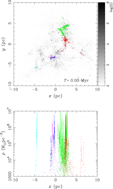
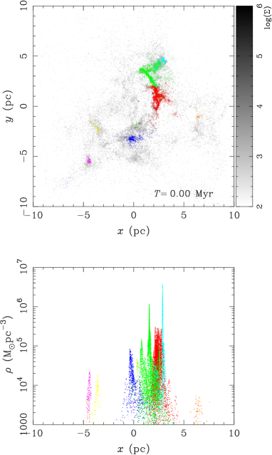
We now investigate the location where the member stars of the clusters formed. In Figure 7 we have colored the initial position of stars that at an age of 10 Myr belong to one cluster. Stars located near each other within a few pc typically merge to one cluster. The density peaks that at 10 Myr still belong to a cluster are presented in the bottom panel of Figure 7. We identify several density peaks, each of which eventually (at an age of 10 Myr) corresponds to one cluster. From the figure we see that a minimum gas density of $\sim 10^{4}M_{\odot}{\rm pc}^{-3}$ is required to form a cluster which survives for 10 Myr. This seems to be related the SFE-law we adopted (see equation (2)). With a gas density of $1.6\times 10^{4}M_{\odot}{\rm pc}^{-3}$, the SFE $\sim 0.5$, and the mass in regions with a density $\ {\raise-2.15277pt\hbox{$\buildrel>\over{\sim}$}}\ 10^{4}M_{\odot}{\rm pc}^{-3}$ are dominated by stars; as a consequence these regions easily survive the gas expulsion.

The relation between the maximum cluster mass and molecular cloud mass does not change appreciable from 2 Myr to 10 Myr. In Figure 6 we plot the results obtained from our simulations and lines for $M_{\rm c,max}=6.3M_{\rm g}^{0.51}$ and $M_{\rm c,max}=0.20M_{\rm g}^{0.76}$.

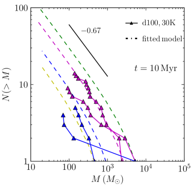
In Fig. 8 we present the mass distribution of star clusters as a function of time. The slope of the cluster mass function becomes shallower between 2 Myr and 10 Myr, even though the smaller number of clusters at later age. At $t=10$ Myr the slope of the cluster MF becomes $\beta=-1.56\pm 0.14$ for the simple fitting to equation (4). If we assume that $M_{\rm c}=M_{\rm c,max}$ obtained from the simulations, we obtain $\beta=-1.53\pm 0.16$. Assuming that $M_{\rm c,max}=0.20M_{\rm g}^{0.76}$, the slope of the cluster MF becomes $\beta=-1.67\pm 0.30$. The best fit parameters for each model are summarized in Table 4. The flatter slope is a natural consequence of the evaporation of the smallest clusters and hierarchical merging, in which lower mass clumps merge to more massive clumps. After 10 Myr clusters stop merging, because the entire system is unbound (see virial ratio of the system in Table 2).

Figure 7: Projected position of stars after the residual gas has been removed. Each color identifies the cluster to which the star belongs at an age of 10 Myr. The data is from model m400k-d100-s1-30K. We used the same colors as in Figure 4. The projected stellar density is presented as a gray scale. In the bottom panel we show the density distribution along one dimension, and gives the same data as is presented in Figure 2, but for SPH particles which are converted to stars. The colors are the same as the top panel. Red, green, blue, cyan, and magenta clusters are relatively massive, and they are 2800, 5300, 690, 360, and 230 $M_{\odot}$, respectively.

Figure 8: Same as Figure 5, but for $t=10$ Myr. We adopt $A=0.63$, $\beta=-1.67$, and $M_{\rm c,max}=0.20M_{\rm g}^{0.76}$ for the fitting MF (see equation (5)).

4 Total Cluster Mass Function in Disk Galaxies

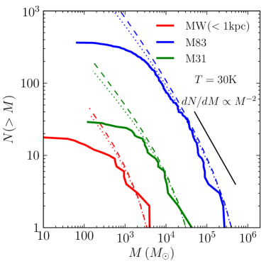
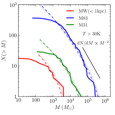
In order to compare our simulations with the observed cluster mass-function in a galactic environment, we assume the GMC mass-function to follow a power-law down to $100M_{\odot}$. We ignore less massive clouds because they are unable to form sufficiently massive clusters to compare with the observations. For the Milky Way we adopt a power of $-1.45$ (Planck Collaboration et al., 2011) and for M31 we adopt $-0.9$ (Kirk et al., 2013). For M82 we also adopt a power of $-1.45$, because there is insufficient data to properly fit the distribution. We assume that each individual GMC forms a conglomerate of clusters that follow equation (5). Here we adopt $\beta=-1.73$ and $A=0.64$ for $t=2$ Myr, $\beta=-1.67$ and $A=0.63$ for $t=10$ Myr, and $M_{\rm c,max}=0.20M_{\rm g}^{0.76}$ for both. As a consequence a distribution of GMCs forms a superposition of multiple cluster mass-functions; one for each GMC in the galaxy. The mass functions for all young clusters in such a galaxy is presented in Figure 9, which we derived using the fitting functions at 2 Myr (dashes) and at 10 Myr (dotted curves). We assume that the total mass of the molecular gas is $2\times 10^{7}M_{\odot}$ and $8\times 10^{8}M_{\odot}$ for M31 and M83, respectively. In this calculation we do not allow any GMC to exceed half the total gas mass in the galaxy. Observationally, the total mass of the molecular gas in each galaxy is $3.6\times 10^{8}M_{\odot}$ for M31 (Nieten et al., 2006) and $2.5\times 10^{9}M_{\odot}$ for M83 (Crosthwaite et al., 2002). For young clusters in the MW and within 1 kpc of the Sun, we derive the total mass in molecular clouds of $10^{6}M_{\odot}$ in order to match the cluster mass function. This indicates that the total mass in molecular clouds within 1 kpc is $\sim 10^{6}M_{\odot}$.

Because of the cut-off in the Schechter mass function, the power-law slope of the superposed mass function is $\ {\raise-2.15277pt\hbox{$\buildrel<\over{\sim}$}}\ -2$. This value is consistent with cluster mass functions observed in nearby galaxies (Portegies Zwart et al., 2010). The solid curves in Figure 9 indicate the observed MF for young clusters in the MW (within a distance of $D=1$kpc from the Sun), M31, and M83. With “young” we here indicate cluster with an age comparable to the typical free-fall time of the GMC in each galaxy. If we consider that GMCs collapse on this timescale and form stars, the free-fall time scale of GMCs would be associated with the star-formation time scale, as was suggested in Krumholz et al. (2012a). The typical free-fall time scale estimated from observations is $\sim 25$ Myr for M31 and $\sim 70$ Myr for M83 (Krumholz et al., 2012a). These values are much longer than the free-fall time scales in our models, but we consider that the final SFE does not change much even if the initial free-fall time scale is longer. For the MW, we adopted a typical value for disk galaxies of 30 Myr. Our model for the total cluster mass function agrees with the observed cluster mass function in the MW, M31, and M83.

We have not considered the evolution of star clusters beyond 10 Myr. At these later ages the cluster-disruption process is expected to continue to change the shape of the cluster mass function (Bastian et al., 2012), in particular by stellar mass loss, internal two-body relaxation and the external influences of the galactic tidal field. Some of the discrepancies between our simulations and the observation are probably caused by our adopted limited time scale of 10 Myr, and by ignoring the global potential of the parent galaxy.

Figure 9: Thick curves indicate the cumulative cluster MF for MW($D<1$kpc, $<30$ Myr), M31($<25$Myr), and M83 ($<70$Myr). Dashed and dotted curves indicate our model given by equation (5) at 2 Myr and at 10 Myr, respectively. Here we adopt $\beta=-1.73$ and $A=0.64$ for $t=2$ Myr, $\beta=-1.67$ and $A=0.63$ for $t=10$ Myr, and $M_{\rm c,max}=0.20M_{\rm g}^{0.76}$ for both. The observational data is from Bastian et al. (2011a, b, 2012) for M83 and Vansevičius et al. (2009) for M31.

5 Discussion

5.1 The Self-Similarity between the Stellar Mass Function and the Cluster Mass Function

The similarity between the cluster mass-function and the stellar mass-function seems to originates from the self-similar structure of GMC, as was also discussed in Elmegreen (2002). From an observational perspective, the relation between the self-similar structure of GMCs and star forming regions has been suggested by (Elmegreen & Falgarone, 1996; Elmegreen & Scalo, 2004; Sánchez et al., 2010). As can be seen in Figure 7, more massive clusters tend to form in densiter regions. If the resolution of our simulation was sufficiently high to resolve the formation of individual stars, we expect to see spikes in the density distribution which correspond to individual stars. We then would expect that more massive stars form in more massive and denser regions. The most massive star will then be born in the most massive cluster in the system. The birth of the most massive star cluster as well as the most massive individual star is then limited by the highest mass and densest GMCs in the MW. A similar argument was discussed in Weidner & Kroupa (2005) and Weidner et al. (2010).

In our simulations we obtain the relation between GMC mass and the maximum cluster mass of $M_{\rm c,max}=6.3M_{\rm g}^{0.51}$ or $M_{\rm c,max}=0.20M_{\rm g}^{0.76}$. If we apply these relations to the Milky Way, in which the most massive GMC is $10^{7}M_{\odot}$ (Murray, 2011), it can form at most a cluster of a few $10^{4}M_{\odot}$, which again forms a single star of at most $\sim 100M_{\odot}$. Note that even if the most massive stars are born in the regions with the highest density, this location is not necessarily associated with the most massive cluster. In this sense, we consider that the $m_{\rm max}$-$M_{\rm c}$ relation is a statistical result, as was suggested earlier by Elmegreen (2006), Bastian et al. (2010), and Bressert et al. (2010).

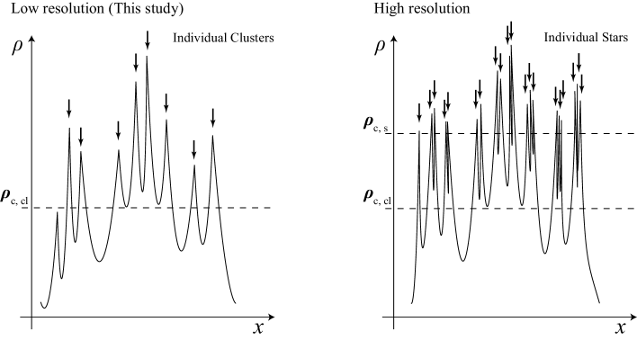
Although we observe a similarity between the largest structures in the system; stellar mass function and cluster mass function, the slopes are somewhat different. In order to follow the formation of individual stars, higher resolution simulations of more massive clusters with the appropriate physics would be required. upon performing such simulations we anticipate that the mass function of individual stars would have a slope consistent with the Salpeter (Salpeter, 1955) slope, as was suggested by (Bonnell et al., 2003; Bate et al., 2003). In Figure 10, we present a schematic picture of the formation of a cluster (left) down to individual stars (right), as we perceive it from our simulations. In a simulations where individual stars remain unresolved clusters can form, but by increasing the resolution more fine-structure in the density distribution of the gas will appear. Those density peaks are associated with individual stars, and groups of peaks are associated with clusters of stars. If the peak density exceeds the critical density for star cluster formation ($\rho_{\rm c,cl}\sim 10^{4}M_{\odot}\mathrm{pc}^{3}$ in our simulation), the cluster survives for at least 10 Myr. Some clusters will merge to a larger and more massive cluster. If we were able to resolve individual star formation, we would resolve the cluster formation peaks to ensembles of peaks that correspond to individual stars.

Figure 10: Schematic representation of the density distribution of the formation process of cluster in relatively low-resolution simulations (left panel) and in an environment where the formation of individual stars is resolved (right).

5.2 Higher Temperature Simulations

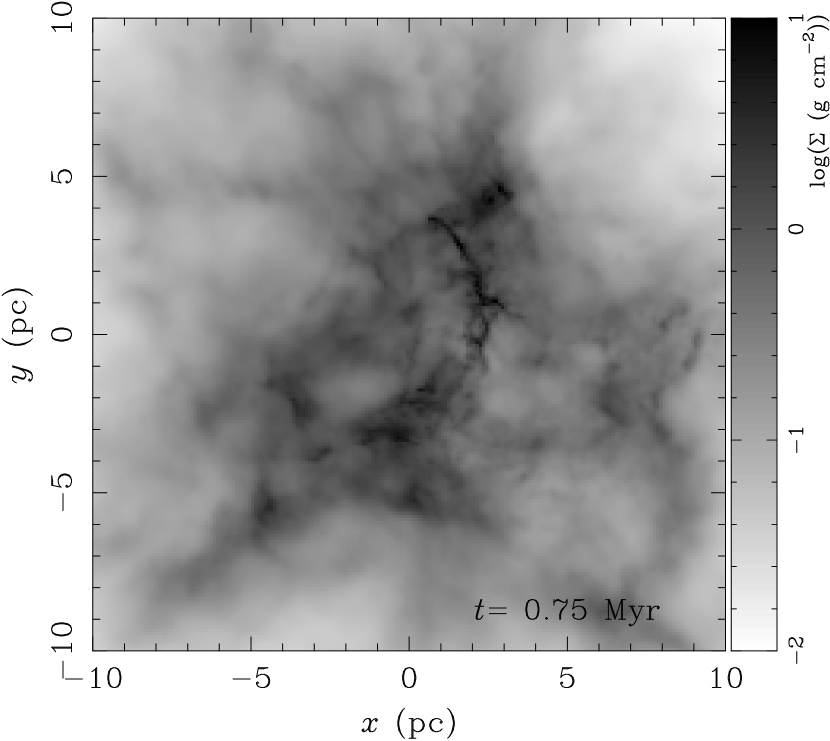
We adopt a temperature of 30K for our standard models, but we also perform a series of simulations with a thermal energy of 1% of the kinetic energy in order to see the effect of the temperature. With this setup, the gas temperature exceed 100 K. The other parameters are the same as models with 30K. The initial conditions of the high temperature models are summarized in Table 5. The structures obtained from the hydro-simulation are considerably smoother because the fragmentation scale is larger at a higher gas temperature. In Figure 11 we present the gas surface density at the end of the hydro-simulation for model m400k-d100-190K, which is almost indistinguishable from m400k-d100-30K, but which has a much higher gas temperature of 190K. The density peaks shown in Figure 12 are less pronounced than in the 30K models (see Figure 2). Although the number of small clumps seen as density peaks in Figure 2 are smaller in the high-temperature simulations, the eventual stellar distributions at 2 or 10 Myr, such as the shape of cluster mass function obtained from the $N$-body simulations was not much affected by the temperature. In Table 6 we summarize the initial conditions for $N$-body simulations.

Table 5: Models for hydrodynamical simulations with higher temperatures (’s’ indicates the random seeds for the turbulence).

Model	Total mass	$N$ of particles	Radius	Density	Thermal Energy	Temperature
	$M_{\rm g}(M_{\odot})$	$N_{\rm g}$	$r_{\rm g}$(pc)	$\rho_{\rm g}({\rm cm}^{-3})$	$E_{\rm t}/E_{\rm k}$	$T$ (K)
m5M-d10-s1-490K	$5\times 10^{6}$	$5\times 10^{6}$	49.0	170	0.01	490
m1M-d100-s1-360K	$1\times 10^{6}$	$1\times 10^{6}$	13.4	$1.7\times 10^{3}$	0.01	360
m1M-d100-s6-360K	$1\times 10^{6}$	$1\times 10^{6}$	13.4	$1.7\times 10^{3}$	0.01	360
m1M-d100-s7-360K	$1\times 10^{6}$	$1\times 10^{6}$	13.4	$1.7\times 10^{3}$	0.01	360
m1M-d10-s1-170K	$1\times 10^{6}$	$1\times 10^{6}$	28.5	170	0.01	170
m1M-d10-s4-170K	$1\times 10^{6}$	$1\times 10^{6}$	28.5	170	0.01	170
m400k-d100-s1-190K	$4\times 10^{5}$	$4\times 10^{5}$	10.0	$1.7\times 10^{3}$	0.01	190
m400k-d100-s2-190K	$4\times 10^{5}$	$4\times 10^{5}$	10.0	$1.7\times 10^{3}$	0.01	190
m400k-d100-s5-190K	$4\times 10^{5}$	$4\times 10^{5}$	10.0	$1.7\times 10^{3}$	0.01	190
m400k-d10-s1-90K	$4\times 10^{5}$	$4\times 10^{5}$	21.0	170	0.01	92
m100k-d100-s1-80K	$1\times 10^{5}$	$1\times 10^{5}$	6.2	$1.7\times 10^{3}$	0.01	78
m40k-d100-s1-40K	$4\times 10^{4}$	$4\times 10^{4}$	4.5	$1.7\times 10^{3}$	0.01	43

Table 6: Models for $N$-body simulations based on higher temperature molecular clouds

Model	Total mass	$N$ of particles	Virial ratio	SFE (Global)	SFE (Dense)
	$M_{\rm s}(M_{\odot})$	$N_{\rm s}$	$Q_{\rm vir}$	$\epsilon$	$\epsilon_{\rm d}$
m5M-d10-s1-490K	$1.6\times 10^{5}$	155972	5.4	0.032	0.25
m1M-d100-s1-360K	$5.8\times 10^{4}$	57642	3.0	0.058	0.20
m1M-d100-s6-360K	$4.1\times 10^{4}$	40510	7.6	0.041	0.13
m1M-d100-s7-360K	$6.9\times 10^{4}$	68901	1.0	0.070	0.19
m1M-d10-s1-170K	$3.1\times 10^{4}$	31023	4.6	0.032	0.18
m1M-d10-s4-170K	$3.6\times 10^{4}$	36224	3.7	0.037	0.30
m400k-d100-s1-190K	$3.2\times 10^{4}$	31868	2.8	0.078	0.26
m400k-d100-s2-190K	$3.0\times 10^{4}$	30496	1.5	0.075	0.22
m400k-d100-s5-190K	$2.5\times 10^{4}$	25419	2.8	0.062	0.19
m400k-d10-s1-90K	$1.5\times 10^{4}$	15124	3.2	0.037	0.35
m100k-d100-s1-80K	$6.4\times 10^{3}$	6474	1.4	0.063	0.20
m40k-d100-s1-40K	$2.5\times 10^{3}$	2498	2.0	0.062	0.19

Figure 11: Gas surface density at an age of $0.9t_{\rm ff}$ for model m400k-d100-190K.

Figure 12: Gas surface density at $0.9t_{\rm ff}$ for model m400k-d100-190K (top panel in gray scale). Colors indicate dense region; cyan, blue, magenta, green indicates regions with the volume density of $>10^{6}$, $10^{5-6}$, $10^{4-5}$, and $10^{3-4}M_{\odot}$pc^-3, respectively. Gas volume density distribution projected on $x$-axis (bottom). Colors are the same as in top panel.

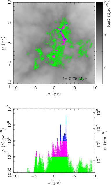
The evolution of the stellar system for model m400k-d100-190K is shown in Figure 13. The position and mass of the clusters formed at 10 Myr in m400k-d100-190K are different that those resulting from model m400k-d100-30K. The stellar composition of the most massive clusters and their initial locations in space is hardly affected by the different temperatures. In Figure 14 we present, for model m400k-d100-190K, the stellar positions that are contained in the five most massive clusters at an age of 10 Myr.

We investigated the cluster MF for these models at $t=2$ and 10 Myr. The resulting cluster MFs are shown in Figures 15 and 16 for $t=2$ and 10 Myr, respectively. We also fit the results to equation (5). The fitted $\beta$ and $A$ for each model are summarized in Tables 7 and 8. When we adopt the actual values of the most massive clusters as $M_{\rm c,max}$ we obtain $\beta=-1.52\pm 0.21$ for the high temperature models, but $\beta=-1.62\pm 0.22$ when we include the 30K models. The mass of the most massive clusters does not much different from those for 30K models. The relation between the initial gas mass and the mass of the most massive cluster is $M_{\rm c,max}=26M_{\rm g}^{0.39}$ at $t=2$ Myr only for high temperature models. By adding artificial points at $M_{\rm c,max}=0.01M_{\odot}$ and $M_{\rm g}=0.02M_{\odot}$, we obtain $M_{\rm c,max}=0.17M_{\rm g}^{0.73}$ at $t=2$ Myr. If we assume $M_{\rm c,max}=0.20M_{\rm g}^{0.76}$ (the same as that obtained in 30K models), we obtain the averaged power-law slope of the fitting function of $\beta=-1.52\pm 0.22$ and $\beta=-1.37\pm 0.20$ at $t=2$ and 10 Myr, respectively. These slopes are slightly shallower than those in the low temperature simulations, but both values are consistent within the uncertainty. We also obtain $A=0.60\pm 0.29$ and $A=0.78\pm 0.34$ at $t=2$ and 10 Myr. With these values, the total cluster MF for galaxies obtained from our model is consistent with the observations (see Figure 17).

Table 7: The results of simulations at $t=2$Myr. For $\beta_{2}$ and $A$, we assume $M_{\rm c,max}=0.20M_{\rm g}^{0.76}$. Averaging the results, we obtain $\beta_{1}=-1.52\pm 0.21$, $\beta_{2}=-1.54\pm 0.16$, and $A=0.60\pm 0.29$ only for high temperature models and $\beta_{1}=-1.62\pm 0.22$, $\beta_{2}=-1.64\pm 0.19$, and $A=0.62\pm 0.28$ for all models including 30K models.

Model	$M_{\rm s,cl}/M_{\rm s}$	$M_{\rm c,max}(M_{\odot})$	$N_{\rm c}$	$\beta_{1}$	$\beta_{2}$	$A$
m5M-d10-s1-490K	0.33	$1.0\times 10^{4}$	27	$-1.61\pm 0.03$	$-1.63\pm 0.03$	$0.37\pm 0.05$
m1M-d100-s1-360K	0.33	$8.4\times 10^{3}$	14	$-1.43\pm 0.06$	$-1.43\pm 0.06$	$0.65\pm 0.15$
m1M-d100-s6-360K	0.34	$4.3\times 10^{3}$	14	$-1.58\pm 0.05$	$-1.62\pm 0.05$	$0.57\pm 0.09$
m1M-d100-s7-360K	0.39	$7.0\times 10^{3}$	29	$-1.52\pm 0.02$	$-1.52\pm 0.02$	$1.24\pm 0.10$
m1M-d10-s1-170K	0.26	$5.2\times 10^{3}$	7	$-1.39\pm 0.06$	$-1.41\pm 0.05$	$0.46\pm 0.09$
m1M-d10-s4-170K	0.21	$2.4\times 10^{3}$	9	$-1.23\pm 0.04$	$-1.40\pm 0.08$	$0.69\pm 0.16$
m400k-d100-s1-190K	0.29	$3.8\times 10^{3}$	14	$-1.59\pm 0.05$	$-1.45\pm 0.05$	$0.76\pm 0.12$
m400k-d100-s2-190K	0.35	$9.1\times 10^{3}$	10	$-1.78\pm 0.15$	$-1.76\pm 0.15$	$0.19\pm 0.09$
m400k-d100-s5-190K	0.37	$1.5\times 10^{3}$	14	$-1.87\pm 0.07$	$-1.85\pm 0.07$	$0.29\pm 0.06$
m400k-d10-s1-90K	0.31	$1.3\times 10^{3}$	7	$-1.16\pm 0.06$	$-1.35\pm 0.08$	$0.81\pm 0.17$
m100k-d100-s1-80K	0.31	$1.3\times 10^{3}$	3	-	-	-
m40k-d100-s1-40K	0.28	$2.1\times 10^{2}$	4	-	-	-

Table 8: The results of simulations at 10Myr. Averaging the results, we obtain $\beta_{1}=-1.36\pm 0.20$, $\beta_{2}=-1.37\pm 0.20$, and $A=0.78\pm 0.34$ for high temperature models and $\beta_{1}=-1.43\pm 0.21$, $\beta_{2}=-1.46\pm 0.27$, and $A=0.73\pm 0.34$ for all models including 30K models. Here, we assume $M_{\rm c,max}=0.20M_{\rm g}^{0.76}$.

Model	$M_{\rm c,max}(M_{\odot})$	$N_{\rm c}$	$\beta_{1}$	$\beta_{2}$	$A$
m1M-d100-s1-360K	$9.4\times 10^{3}$	9	$-1.31\pm 0.07$	$-1.55\pm 0.04$	$0.55\pm 0.08$
m1M-d100-s6-360K	$4.0\times 10^{3}$	14	$-1.43\pm 0.04$	$-1.22\pm 0.07$	$0.79\pm 0.18$
m1M-d10-s1-170K	$2.9\times 10^{3}$	5	$-1.08\pm 0.05$	$-1.37\pm 0.05$	$0.88\pm 0.17$
m1M-d10-s4-170K	$2.2\times 10^{3}$	12	$-1.22\pm 0.03$	$-1.07\pm 0.11$	$1.28\pm 0.49$
m400k-d100s1-190K	$4.1\times 10^{3}$	8	$-1.24\pm 0.08$	$-1.23\pm 0.08$	$1.18\pm 0.30$
m400k-d100-s2-190K	$9.3\times 10^{3}$	8	$-1.70\pm 0.09$	$=1.68\pm 0.17$	$0.20\pm 0.11$
m400k-d100-s5-190K	$4.9\times 10^{3}$	13	$-1.41\pm 0.05$	$=1.49\pm 0.08$	$0.61\pm 0.15$
m100k-d100-s1-80K	$1.2\times 10^{3}$	4	-	-	-
m40k-d100-s1-40K	$3.2\times 10^{2}$	3	-	-	-

The high temperature we assumed here ($>100$K) is not realistic for a model of molecular clouds. The main clusters formed from initial conditions with a high temperature, however, are not much different from those formed from molecular cloud with a realistic temperature. In low-temperature models, there are more clumps in a region which finally merge to a cluster. The clumps merge within a local dynamical time scale irrespective of the gas temperature. The clumpy structure is lost quickly in the merger process, mainly due to violent relaxation. The formation of massive cluster is therefore not affected by the unrealistically high temperature of the gas. This result is practical when applying this same method to a cluster formation simulations on a galactic scale. In evironments where temperature of $\ {\raise-2.15277pt\hbox{$\buildrel>\over{\sim}$}}\ 100$ K are reached, which is a quite typical threshold temperature of star forming regions in galaxy simulations, the temperature is sufficiently low to result in clustered star formation. In those cases we do not necessarily resolve the low-temperature and high density regions.

Figure 13: The snapshots of the $N$-body simulation for model m400k-d100-190K.

Figure 14: Projected position of stars after the residual gas has been removed. Each color identifies the cluster to which the star belongs at an age of 10 Myr. The data is from model m400k-d100-190K. We used the same colors as in Figure 4. The stellar surface density is presented as a gray scale. In the bottom panel we show the density distribution along one dimension, and gives the same data as is presented in Figure 2, but for SPH particles which are converted to stars. The colors are the same as the top panel. Red, green, blue, cyan, and magenta clusters are relatively massive, and they are 4100, 3400, 760, 920, and 123 $M_{\odot}$, respectively.

Figure 15: Same as Figure 5, but for models with $>30$K. The colors represent different masses of initial molecular clouds: orange, green, magenta, blue, and yellow indicate $M_{\rm g}$ of $5\times 10^{6},10^{6},4\times 10^{5},10^{5}$ and $4\times 10^{4}M_{\odot}$, respectively. The dashed curves give the fitted MF (see equation (5)). We adopt $A=0.60$, $\beta=-1.54$, and $M_{\rm c,max}=0.20M_{\rm g}^{0.76}$.

Figure 16: Same as Figure 8, but for models with $>30$K. The dashed curves give the fitted MF (see equation (5)). We adopt $A=0.78$, $\beta=-1.37$, and $M_{\rm c,max}=0.20M_{\rm g}^{0.76}$.

Figure 17: Same as Figure 9 but for high temperature models. Here we adopt $\beta=-1.52$ and $A=0.60$ for $t=2$ Myr (dashed lines) and $\beta=-1.37$ and $A=0.78$ for $t=10$ Myr (dotted lines), respectively, and adopt $M_{\rm c,max}=0.20M_{\rm g}^{0.76}$ for both.

6 Summary

We performed $N$-body simulations of ensembles of young star clusters. The initial conditions of our dynamical simulations are obtained from smoothed particles hydrodynamical simulations of turbulent molecular clouds. Both calculations, the collapsing molecular cloud and the gravitational dynamical simulations, are performed individually and are separated. As a result, our calculations are not self consistent, but there is a natural causality.

In our approach we start with the hydrodynamical simulation, which we continue for about a free-fall time scale. We subsequently analyze the distribution of the gas and assign stellar mass to individual SPH particles. In this procedure, mass is locally not conserved, but globally it is. Only those SPH particles that have a local density in excess of the star formation threshold are assumed to form star. This procedure of adopting a simple density threshold results in a local (core) star-formation efficiency of about 30 per-cent, but only about 1 per cent of the total mass in gas is converted to stars. Individual stars are assigned the positions and velocities of the SPH particles from which they were generated. These mass, positions and velocities are adopted as the initial conditions for the gravitational dynamics simulations.

The distribution of stars resulting from this procedure show a strong hierarchical structure. The distribution of the mass of the stellar clumps are consistent with the Schechter function. In the first 2 Myr, after the stars formed, the mass function of clusters resemblances a power-law with a slope of $\simeq-1.73$. This slope becomes shallower with time because of hierarchical merging, to reach a slope of $\simeq-1.67$ at an age of 10 Myr.

The shape of the cluster mass function in our simulations is consistent with the one observed in active star forming regions in the Milky Way, such as in the Carina region. We find a relation between the mass of the GMC and the most massive cluster: $6.3M_{\rm g}^{0.51}$ (or $0.20M_{\rm g}^{0.76}$ if we assume that this relation continues down to the stellar mass scale). This relation is consistent with the observed cluster distribtion in M51 (Hughes et al., 2013), and it is similar to the observed relation between the most massive star and the total mass of the cluster (Weidner et al., 2010). We therefore conclude that star-forming regions and star cluster-forming regions have a self-similar structure down to the formation of individual stars.

Using our simulations we estimate the global galactic cluster MF in the MW, M31, and M83. We satisfactory fitted the distribution of cluster masses for each of these galaxies. The galactic cluster MFs obtained from our model have a power of $\ {\raise-2.15277pt\hbox{$\buildrel<\over{\sim}$}}\ -2$, which is consistent with observed cluster MF nearby galaxies.

References

- André et al. (2010) André P., Men’shchikov A., Bontemps S., Könyves V., Motte F., Schneider N., Didelon P., Minier V., Saraceno P., Ward-Thompson D., di Francesco J., White G., Molinari S., Testi L., Abergel A., Griffin M., Henning T., Royer P., Merín B., Vavrek R., Attard M., Arzoumanian D., Wilson C. D., Ade P., Aussel H., Baluteau J.-P., Benedettini M., Bernard J.-P., Blommaert J. A. D. L., Cambrésy L., Cox P., di Giorgio A., Hargrave P., Hennemann M., Huang M., Kirk J., Krause O., Launhardt R., Leeks S., Le Pennec J., Li J. Z., Martin P. G., Maury A., Olofsson G., Omont A., Peretto N., Pezzuto S., Prusti T., Roussel H., Russeil D., Sauvage M., Sibthorpe B., Sicilia-Aguilar A., Spinoglio L., Waelkens C., Woodcraft A., Zavagno A., 2010, A&A, 518, L102
- Bastian et al. (2011a) Bastian N., Adamo A., Gieles M., Lamers H. J. G. L. M., Larsen S. S., Silva-Villa E., Smith L. J., Kotulla R., Konstantopoulos I. S., Trancho G., Zackrisson E., 2011a, VizieR Online Data Catalog, 741, 79006
- Bastian et al. (2011b) —, 2011b, MNRAS, 417, L6
- Bastian et al. (2012) Bastian N., Adamo A., Gieles M., Silva-Villa E., Lamers H. J. G. L. M., Larsen S. S., Smith L. J., Konstantopoulos I. S., Zackrisson E., 2012, MNRAS, 419, 2606
- Bastian et al. (2010) Bastian N., Covey K. R., Meyer M. R., 2010, ARA&A, 48, 339
- Bate (2012) Bate M. R., 2012, MNRAS, 419, 3115
- Bate et al. (2003) Bate M. R., Bonnell I. A., Bromm V., 2003, MNRAS, 339, 577
- Bonnell et al. (2003) Bonnell I. A., Bate M. R., Vine S. G., 2003, MNRAS, 343, 413
- Bonnell et al. (2008) Bonnell I. A., Clark P., Bate M. R., 2008, MNRAS, 389, 1556
- Bonnell et al. (2011) Bonnell I. A., Smith R. J., Clark P. C., Bate M. R., 2011, MNRAS, 410, 2339
- Bonnell et al. (2004) Bonnell I. A., Vine S. G., Bate M. R., 2004, MNRAS, 349, 735
- Bressert et al. (2010) Bressert E., Bastian N., Gutermuth R., Megeath S. T., Allen L., Evans II N. J., Rebull L. M., Hatchell J., Johnstone D., Bourke T. L., Cieza L. A., Harvey P. M., Merin B., Ray T. P., Tothill N. F. H., 2010, MNRAS, 409, L54
- Crosthwaite et al. (2002) Crosthwaite L. P., Turner J. L., Buchholz L., Ho P. T. P., Martin R. N., 2002, AJ, 123, 1892
- Eisenstein & Hut (1998) Eisenstein D. J., Hut P., 1998, ApJ, 498, 137
- Elmegreen (2002) Elmegreen B. G., 2002, ApJ, 577, 206
- Elmegreen (2006) —, 2006, ApJ, 648, 572
- Elmegreen & Falgarone (1996) Elmegreen B. G., Falgarone E., 1996, ApJ, 471, 816
- Elmegreen & Scalo (2004) Elmegreen B. G., Scalo J., 2004, ARA&A, 42, 211
- Federrath & Klessen (2012) Federrath C., Klessen R. S., 2012, ApJ, 761, 156
- Feigelson et al. (2011) Feigelson E. D., Getman K. V., Townsley L. K., Broos P. S., Povich M. S., Garmire G. P., King R. R., Montmerle T., Preibisch T., Smith N., Stassun K. G., Wang J., Wolk S., Zinnecker H., 2011, ApJS, 194, 9
- Fujii et al. (2009) Fujii M., Iwasawa M., Funato Y., Makino J., 2009, ApJ, 695, 1421
- Fujii & Portegies Zwart (2011) Fujii M. S., Portegies Zwart S., 2011, Science, 334, 1380
- Fujii et al. (2012) Fujii M. S., Saitoh T. R., Portegies Zwart S. F., 2012, ApJ, 753, 85
- Gerritsen & Icke (1997) Gerritsen J. P. E., Icke V., 1997, A&A, 325, 972
- Hernquist & Katz (1989) Hernquist L., Katz N., 1989, ApJS, 70, 419
- Hughes et al. (2013) Hughes A., Meidt S. E., Schinnerer E., Colombo D., Pety J., Leroy A. K., Dobbs C. L., García-Burillo S., Thompson T. A., Dumas G., Schuster K. F., Kramer C., 2013, ApJ, 779, 44
- Hurley et al. (2000) Hurley J. R., Pols O. R., Tout C. A., 2000, MNRAS, 315, 543
- Keto & Wood (2006) Keto E., Wood K., 2006, ApJ, 637, 850
- King (1966) King I. R., 1966, AJ, 71, 64
- Kirk et al. (2013) Kirk J. M., Gear W. K., Fritz J., Smith M. W. L., Ford G., Baes M., Bendo G. J., De Looze I., Eales S. A., Gentile G., Gomez H. L., Gordon K., O’Halloran B., Madden S. C., Duval J. R., Verstappen J., Viaene S., Boselli A., Cooray A., Lebouteiller V., Spinoglio L., 2013, ArXiv e-prints
- Kruijssen et al. (2012) Kruijssen J. M. D., Maschberger T., Moeckel N., Clarke C. J., Bastian N., Bonnell I. A., 2012, MNRAS, 419, 841
- Krumholz (2012) Krumholz M. R., 2012, ApJ, 759, 9
- Krumholz et al. (2012a) Krumholz M. R., Dekel A., McKee C. F., 2012a, ApJ, 745, 69
- Krumholz et al. (2012b) Krumholz M. R., Klein R. I., McKee C. F., 2012b, ApJ, 754, 71
- Krumholz & Thompson (2012) Krumholz M. R., Thompson T. A., 2012, ApJ, 760, 155
- Lada & Lada (2003) Lada C. J., Lada E. A., 2003, ARA&A, 41, 57
- Larson (2003) Larson R. B., 2003, in Astronomical Society of the Pacific Conference Series, Vol. 287, Galactic Star Formation Across the Stellar Mass Spectrum, De Buizer J. M., van der Bliek N. S., eds., pp. 65–80
- McKee & Ostriker (2007) McKee C. F., Ostriker E. C., 2007, ARA&A, 45, 565
- Moeckel & Bate (2010) Moeckel N., Bate M. R., 2010, MNRAS, 404, 721
- Moeckel et al. (2012) Moeckel N., Holland C., Clarke C. J., Bonnell I. A., 2012, MNRAS, 425, 450
- Murray (2011) Murray N., 2011, ApJ, 729, 133
- Nieten et al. (2006) Nieten C., Neininger N., Guélin M., Ungerechts H., Lucas R., Berkhuijsen E. M., Beck R., Wielebinski R., 2006, A&A, 453, 459
- Nitadori & Makino (2008) Nitadori K., Makino J., 2008, New Astronomy, 13, 498
- Parker et al. (2014) Parker R. J., Wright N. J., Goodwin S. P., Meyer M. R., 2014, MNRAS, 438, 620
- Pelupessy (2005) Pelupessy F. I., 2005, PhD thesis, Leiden Observatory, Leiden University, P.O. Box 9513, 2300 RA Leiden, The Netherlands
- Pelupessy et al. (2004) Pelupessy F. I., van der Werf P. P., Icke V., 2004, A&A, 422, 55
- Pelupessy et al. (2013) Pelupessy F. I., van Elteren A., de Vries N., McMillan S. L. W., Drost N., Portegies Zwart S. F., 2013, A&A, 557, A84
- Peters et al. (2010) Peters T., Banerjee R., Klessen R. S., Mac Low M.-M., Galván-Madrid R., Keto E. R., 2010, ApJ, 711, 1017
- Pflamm-Altenburg et al. (2007) Pflamm-Altenburg J., Weidner C., Kroupa P., 2007, ApJ, 671, 1550
- Piskunov et al. (2008) Piskunov A. E., Kharchenko N. V., Schilbach E., Röser S., Scholz R.-D., Zinnecker H., 2008, A&A, 487, 557
- Planck Collaboration et al. (2011) Planck Collaboration, Ade P. A. R., Aghanim N., Arnaud M., Ashdown M., Aumont J., Baccigalupi C., Balbi A., Banday A. J., Barreiro R. B., et al., 2011, A&A, 536, A23
- Plummer (1911) Plummer H. C., 1911, MNRAS, 71, 460
- Portegies Zwart & Boekholt (2014) Portegies Zwart S., Boekholt T., 2014, ApJ, 785, L3
- Portegies Zwart et al. (2009) Portegies Zwart S., McMillan S., Harfst S., Groen D., Fujii M., Nualláin B. Ó., Glebbeek E., Heggie D., Lombardi J., Hut P., Angelou V., Banerjee S., Belkus H., Fragos T., Fregeau J., Gaburov E., Izzard R., Jurić M., Justham S., Sottoriva A., Teuben P., van Bever J., Yaron O., Zemp M., 2009, New A, 14, 369
- Portegies Zwart et al. (2013) Portegies Zwart S., McMillan S. L. W., van Elteren E., Pelupessy I., de Vries N., 2013, Computer Physics Communications, 183, 456
- Portegies Zwart et al. (2010) Portegies Zwart S. F., McMillan S. L. W., Gieles M., 2010, ARA&A, 48, 431
- Sabbi et al. (2012) Sabbi E., Lennon D. J., Gieles M., de Mink S. E., Walborn N. R., Anderson J., Bellini A., Panagia N., van der Marel R., Maíz Apellániz J., 2012, ApJ, 754, L37
- Salpeter (1955) Salpeter E. E., 1955, ApJ, 121, 161
- Sánchez et al. (2010) Sánchez N., Añez N., Alfaro E. J., Crone Odekon M., 2010, ApJ, 720, 541
- Springel & Hernquist (2002) Springel V., Hernquist L., 2002, MNRAS, 333, 649
- Toonen et al. (2012) Toonen S., Nelemans G., Portegies Zwart S., 2012, A&A, 546, A70
- Vansevičius et al. (2009) Vansevičius V., Kodaira K., Narbutis D., Stonkutė R., Bridžius A., Deveikis V., Semionov D., 2009, ApJ, 703, 1872
- Weidner & Kroupa (2005) Weidner C., Kroupa P., 2005, ApJ, 625, 754
- Weidner et al. (2010) Weidner C., Kroupa P., Bonnell I. A. D., 2010, MNRAS, 401, 275
- Zapata et al. (2008) Zapata L. A., Palau A., Ho P. T. P., Schilke P., Garrod R. T., Rodríguez L. F., Menten K., 2008, A&A, 479, L25
- Zinnecker & Yorke (2007) Zinnecker H., Yorke H. W., 2007, ARA&A, 45, 481