Achieving High Performance with Unified Residual Evaluation

Abstract

We examine residual evaluation, perhaps the most basic operation in numerical simulation. By raising the level of abstraction in this operation, we can eliminate specialized code, enable optimization, and greatly increase the extensibility of existing code.

1 Introduction

With modern partial differential equation (PDE) solver packages, only performance-critical code the application developers must write is the “physics”, that is, the residual form of the PDE they wish to solve. All the mesh management and algebraic solver code can be contained in highly optimized libraries. To obtain high performance on modern computer systems, however, requires minimizing memory motion, full threading, and fully vectorizable code. Missing even one of the three could immediately decrease the speed of the code by an order of magnitude. How can application developers without computer science expertise write residual code that can be achieve high performance?

At one end, with the FEniCS project [5, 4, 8] the scientist writes no code at all, just a symbolic representation of the weak form of the PDE. Internally FEniCS relies on code generation and separate library routines, rather than a single method for element traversal and integration to compute the residual. This approach increases the complexity of the underlying code, however, and has made it too difficult to support mixed-topology meshes and block-decomposed solvers, as well as to implement implicit material models such as plasticity or real gases or to reuse legacy code. Other work such as AceGen [12] has focused on code generation for complex material models across a limited selection of discretizations. At the other end of the spectrum, with lower-level libraries such as libMesh [9] and Deal.II [2], the scientist writes the required traversal over elements, basis functions, and quadrature points; hence a new routine is constructed for each application, and the scientist is required to ensure that it is high performing. This low-level interface is flexible, allowing the user to implement custom stabilization, choose various implementations of boundary conditions (e.g., slip), implement delta functions, under-integrate certain terms, and countless other forms of messiness in finite element methods. The user’s code is formally independent of the element topology, basis, and quadrature, but the naive representation of basis evaluation is baked into the interface. MOOSE [7, 6, 14] takes a framework approach, with the goal of creating extensive libraries of physical systems and material models to be used with different classes of physical problems (phase-field, elasticity, fluids, etc.) that are coupled together at runtime into multiphysics simulations. Most MOOSE users spend their time working on material models and/or coupling various physical systems together, though some create new classes of physical problems. MOOSE’s approach is extremely dynamic, allowing all composition and model configuration to be specified at run-time, but the interface is too fine-grained to vectorize with current compiler technology. Note that there has been a long tradition in specific problem domains, most notably structural analysis (see FEAP [13] and commercial packages such as Abaqus) of incorporating extensibility in FEM software via “elements” containing the discretization and general structure of the PDE, and “materials” providing closures such as the stress-strain relationship. This organization of material models is compatible with MOOSE (indeed, Abaqus UMAT files can be used directly); but generic coupling and implementing new models and discretizations is high-effort or unsupported.

We propose an alternative somewhere between these two extremes: the scientist provides point function evaluations while the library is responsible for iterating over the mesh elements and quadrature points. We call this approach “unified” because we do not need to write different iteration schemes in the library for different mesh entities, dimensions, discretizations, and the like, as is usually done. Our approach offers three benefits.

Flexibility Our unified formulation of residual evaluation greatly increases the flexibility of simulation code. The cell traversal handles arbitrary cell shape (such as simplicial, tensor product, or polygonal) and hybrid meshes. Moreover, the problem can be posed in any spatial dimension with an arbitrary number of physical fields. It also accommodates general discretizations, tabulated with a given quadrature rule.

Extensibility The library developer needs to maintain only a single method, rather than a code generation engine or a vast collection of specialized routines, easing language transitions and other environmental changes. Moreover, extensibility becomes much easier since a new user must master only a small piece of code in order to contribute to the package. For example, a new discretization scheme could be enabled in a single place in the code.

Efficiency A prime motivation for refactoring residual evaluation is to enable stronger, targeted optimization. In this formulation, only a single routine need be optimized. In addition, the user, application scientist, or library builder is no longer responsible for proper vectorization, tiling, and other traversal optimization.

We can also enable performance portability of an entire application by recoding a single routine for new hardware. For example, we have produced OpenCL and CUDA versions of our FEM residual evaluation that achieve excellent performance on a range of many-core architectures [11].

2 Implementation

We will describe in detail the implementation of a generic residual evaluation method for finite element problems. Our basic operation will be integration of a weak form over a chunk of cells. For a CPU, each chunk is executed in serial and corresponds to classic tiling for cache reuse. On an accelerator, a separate block of threads will execute each chunk in parallel. Moreover, in our CUDA and OpenCL implementations, a chunk is further subdivided into batches that are processed in serial. The batches are then subdivided into blocks that are processed concurrently by groups of threads. However, the subdivision of the iteration space and resulting traversals, including those over basis functions and quadrature points, are handled by the library rather than the user, as discussed below.

At the highest level, we first map all global input vectors to local vectors, using the PETSc DMGlobalToLocal() function. The local space contains unknowns constrained by Dirichlet conditions and shared unknowns on process boundaries that are not present in the global vector used by the solver. In addition, the boundary values are set in the local solution input vector. For each cell chunk, we extract the input, such as solution FEM coefficients, cell geometry, and auxiliary field coefficients, then perform the form integration, and insert the result back into the local residual vector. The local residual then is accumulated into the global residual vector using by DMLocalToGlobal().

The first serious complication comes when extracting FEM coefficients for a cell chunk. The PETSc unstructured mesh interface [10, 1] uses a Hasse diagram [15] to represent the mesh and provides a topological interface independent of the spatial dimension or shape of the constituents, using the PETSc DMPlex class. We can ask for a given breadth-first level in the DAG representing the mesh. For example, cells are leaves of the DAG and thus have height zero, whereas vertexes have depth zero. These are similar to the concepts of dimension and codimension, but they arise naturally from the representation. We can prescribe the data layout for any discretization using a simple size-offset map over all the points in the mesh DAG, called a PetscSection. For example, a 3D $P_{2}$ Lagrange element would have one degree of freedom (dof) on each vertex and edge in the mesh. We can then replace continuum geometric notions with their discrete counterparts to enable generic traversals. In our FEM example, the continuum closure is replaced by the transitive closure over the mesh DAG, where we stack up dofs as we encounter each point based on the PetscSection mapping. Below we show how all these ingredients are used to implement generic coefficient extraction.

  DM           dm;  Vec          X;  PetscSection section;  PetscScalar *x, *u;  PetscInt     cStart, cEnd, c, n, i, off = 0;  DMPlexGetHeightStratum(dm, 0, &cStart, &cEnd);  for (c = cStart; c < cEnd; ++c) {    DMPlexVecGetClosure(dm, section, X, c, &n, &x);    for (i = 0; i < n; ++i, ++off) u[off+i] = x[i];    DMPlexVecRestoreClosure(dm, section, X, c, &n, &x);  }A slight complication arises for multiple fields, which the PetscSection can view as separate maps. Originally, all dofs associated with a given mesh point are stored contiguously in the global and local vectors. The DMPlexVecGetClosure() method reorders the dofs returned so that each field is contiguous.

The code above will not change for different spatial dimensions, number of fields, cell shapes, mesh topologies, or discretizations. Thus, we can reuse the same code to extract geometric data just by replacing section by the layout of coordinate dofs. After all integration has been carried out, we can use the complementary function DMPlexVecSetClosure() to place the residual element vectors into the local residual vector.

   for (c = cStart; c < cEnd; ++c) {    off = c*cellDof;    DMPlexVecSetClosure(dm, section, F, c, &elemVec[off], ADD_VALUES);  }

We have now reduced the problem of residual evaluation to the integration of a weak form over a small chunk of cells. We will introduce a simple model of FEM residual evaluation,

$$\mathbf{\phi^{T}F(u)}\sim\int_{\Omega}\phi\cdot f_{0}(u,\nabla u)+\nabla\phi:{\bf f}_{1}(u,\nabla u)=0,$$ (1)

where the pointwise functions $f_{0},{\bf f}_{1}$ capture the problem physics. Discretizing, we have

$$\mathsf{F(u)}\sim\sum_{e}\mathcal{E}^{T}_{e}\left[B^{T}Wf_{0}(u^{q},\nabla u^{q})+\sum_{k}D^{T}_{k}W{\bf f}^{k}_{1}(u^{q},\nabla u^{q})\right]=0,$$ (2)

where $u^{q}$ is the vector of field evaluations at the set $q$ of quadrature points on an element, $W$ is the diagonal matrix of quadrature weights, $B$ and $D$ are basis function matrices that reduce over quadrature points, and $\mathcal{E}_{e}$ is the element restriction operator. This approach can be trivially extended to higher orders by adding terms with more pointwise functions. Using this model, along with automated tabulation of basis functions and derivatives at quadrature points, the user need only specify physics using pointwise functions similar to the strong form problem. In this way, we decouple the problem specification from mesh and dof traversal. The Jacobian of (2) needs only derivatives of the pointwise functions,

$$\mathsf{F^{\prime}(u)}\sim\sum_{e}\mathcal{E}_{e}^{T}\begin{bmatrix}B^{T}&\mathbf{D}^{T}\end{bmatrix}\mathbf{W}\begin{bmatrix}f_{0,0}&f_{0,1}\\ {\bf f}_{1,0}&{\bf f}_{1,1}\end{bmatrix}\begin{bmatrix}B\\ \mathbf{D}\end{bmatrix}\mathcal{E}_{e}, \quad[f_{i,j}]=\begin{bmatrix}\dfrac{\partial f_{0}}{\partial u}&\dfrac{\partial f_{0}}{\partial\nabla u}\\[10.00002pt] \dfrac{\partial{\bf f}_{1}}{\partial u}&\dfrac{\partial{\bf f}_{1}}{\partial\nabla u}\end{bmatrix}(u,\nabla u)$$ (3)

For a chunk of elements we may calculate the element residual vectors according to the following pseudo-code. where we have highlighted opportunities for vectorization:

for chunk in mesh:
	for c in chunk:			vectorize over cells
		$u^{e}$ = closure(c, U)
			$u^{q}$ = $Bu^{e}$	vectorize over quadrature points
			$\nabla u^{q}$ = $Du^{e}$
			$f_{0}(u^{q},\nabla u^{q})$ and $f_{1}(u^{q},\nabla u^{q})$
		$f^{e}=B^{T}Wf_{0}+D^{T}Wf_{1}$		vectorize over basis functions
		closure(c, F) += $f^{e}$

Note that this is the only code that must be ported to new architectures in order to realize all the gains cited above. In recent work [11], the OpenCL implementation of cell chunk integration was used to do residual evaluation on several accelerator architectures, including Nvidia, ATI, and Intel MIC. We employed mixed vectorization over both quadrature points and basis functions. For the Nvidia GTX580 in particular, we achieve almost 300 GF/s for a first-order discretization. In Fig. 1 (see [3]) we see that unassembled operator application greatly reduces memory bandwidth requirements while being competitive in terms of flops for all but lowest order discretizations. Preconditioning will also be required, for which low-order embedded methods are an unintrusive approach. Experiments with the dual order implementation Dohp have shown that a generic variable-order tensor-product implementation can be at least as efficient at all orders as the libMesh and Deal.II implementations, which are based on traditionally-assembled element routines.

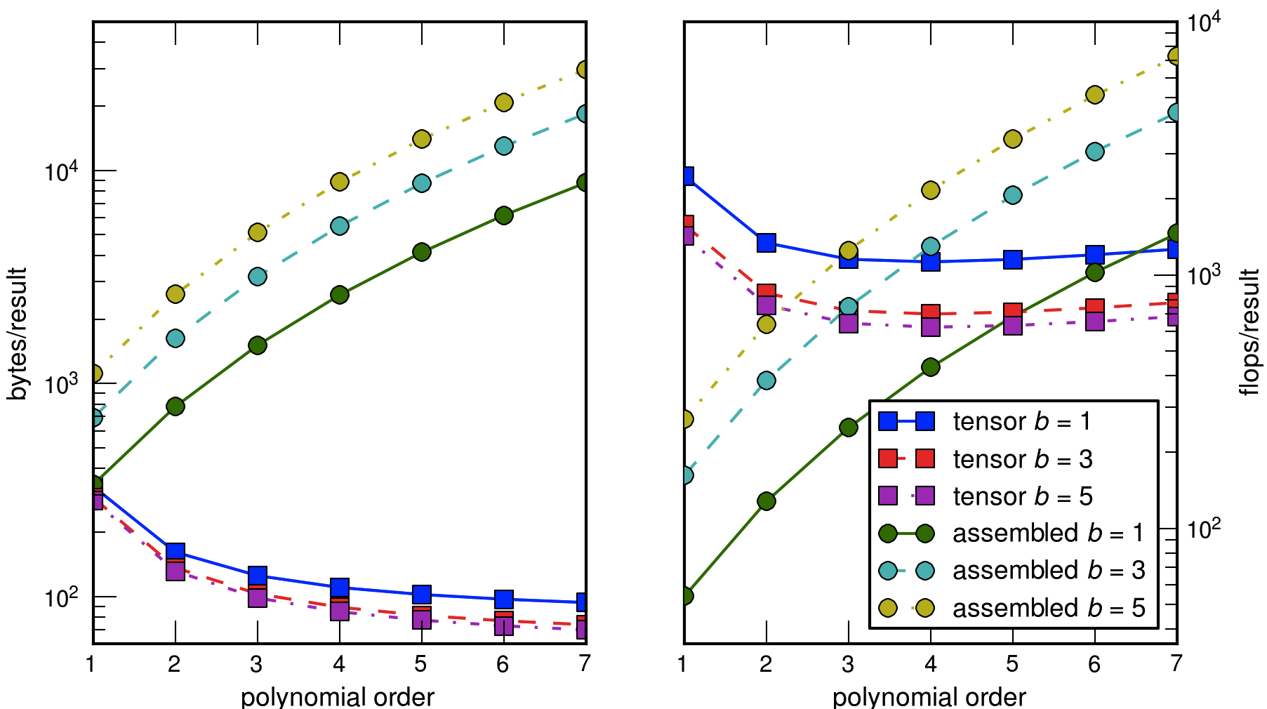
Figure 1: Memory bandwidth and flops per dof to apply a Jacobian from $Q_{k}$ discretization of a $b$-variable PDE system using an assembled matrix versus matrix-free exploiting the tensor product structure in (3).

We are extending this model to pointwise Riemann solvers for hyperbolic conservation laws. The integration would now take place over faces instead of cells, which means we must allow an input cell height for our traversal. Moreover, we update the support of the cell, which is the dual of its closure. The traversal also becomes more complicated when using reconstruction, since this requires a cell traversal as well. However, it seems clear that the model can be generalized to accommodate these changes while maintaining both its simplicity and its efficiency.

Acknowledgments MGK acknowledges partial support from DOE Contract DE-AC02-06CH11357 and NSF Grant OCI-1147680. JB and BFS were support by the U.S. Department of Energy, Office of Science, Advanced Scientific Computing Research, under Contract DE-AC02-06CH11357.

Government License. The submitted manuscript has been created by UChicago Argonne, LLC, Operator of Argonne National Laboratory (“Argonne”). Argonne, a U.S. Department of Energy Office of Science laboratory, is operated under Contract No. DE-AC02-06CH11357. The U.S. Government retains for itself, and others acting on its behalf, a paid-up nonexclusive, irrevocable worldwide license in said article to reproduce, prepare derivative works, distribute copies to the public, and perform publicly and display publicly, by or on behalf of the Government.

References

- [1] B. T. Aagaard, M. G. Knepley, and C. A. Williams. A domain decomposition approach to implementing fault slip in finite-element models of quasi-static and dynamic crustal deformation. Journal of Geophysical Research: Solid Earth, 118(6):3059–3079, 2013. http://dx.doi.org/10.1002/jgrb.50217.
- [2] W. Bangerth, R. Hartmann, and G. Kanschat. deal.II—A general-purpose object-oriented finite element library. ACM Transactions on Mathematical Software (TOMS), 33(4):24–es, 2007.
- [3] Jed Brown. Efficient nonlinear solvers for nodal high-order finite elements in 3D. Journal of Scientific Computing, 45:48–63, 2010.
- [4] T. Dupont, J. Hoffman, J. Jansson, C. Johnson, R. C. Kirby, M. Knepley, M. Larson, A. Logg, and R. Scott. FEniCS Web Page, 2005. http://www.fenicsproject.org.
- [5] T. Dupont, J. Hoffman, C. Johnson, R. C. Kirby, M. G. Larson, A. Logg, and L. R. Scott. The FEniCS project. Technical Report 2003–21, Chalmers Finite Element Center Preprint Series, 2003.
- [6] D. Gaston, G. Hansen, S. Kadioglu, D. Knoll, C. Newman, H. Park, C. Permann, and W. Taitano. Parallel multiphysics algorithms and software for computational nuclear engineering. J. Phys.: Conf. Ser., 180:012012, 2009.
- [7] D. Gaston, C. Newman, G. Hansen, and D. Lebrun-Grandie. MOOSE: A parallel computational framework for coupled systems of nonlinear equations. Nuclear Engineering and Design, 239(10):1768 – 1778, 2009.
- [8] R. C. Kirby, M. G. Knepley, A. Logg, L. R. Scott, and A. R. Terrel. Discrete optimization of finite element matrix evaluation. In Automated solutions of differential equations by the finite element method, volume 84 of Lecture Notes in Computational Science and Engineering, pages 385–397. Springer-Verlag, 2012.
- [9] B. S. Kirk, J. W. Peterson, R. H. Stogner, and G. F. Carey. libMesh: A C++ Library for Parallel Adaptive Mesh Refinement/Coarsening Simulations. Engineering with Computers, 22(3–4):237–254, 2006. http://dx.doi.org/10.1007/s00366-006-0049-3.
- [10] M. G. Knepley and D. A. Karpeev. Mesh algorithms for PDE with Sieve I: Mesh distribution. Scientific Programming, 17(3):215–230, 2009. http://arxiv.org/abs/0908.4427.
- [11] M. G. Knepley, K. Rupp, and A. R. Terrel. Finite element integration with quadrature on accelerators. 2013.
- [12] J. Korelc. Multi-language and multi-environment generation of nonlinear finite element codes. Engineering with Computers, 18(4):312–327, 2002.
- [13] R. L. Taylor. FEAP: A finite element analysis program. Technical report, University of California, Berkeley, 2011.
- [14] M.R. Tonks, D. Gaston, P.C. Millett, D. Andrs, and P. Talbot. An object-oriented finite element framework for multiphysics phase field simulations. Computational Materials Science, 51(1):20–29, 2012.
- [15] Wikipedia. Hasse diagram, 2010. http://en.wikipedia.org/wiki/Hasse_diagram.