Understanding shape entropy through local dense packing

Abstract

Entropy drives the phase behavior of colloids ranging from dense suspensions of hard spheres or rods to dilute suspensions of hard spheres and depletants. Entropic ordering of anisotropic shapes into complex crystals, liquid crystals, and even quasicrystals has been demonstrated recently in computer simulations and experiments. The ordering of shapes appears to arise from the emergence of directional entropic forces (DEFs) that align neighboring particles, but these forces have been neither rigorously defined nor quantified in generic systems. Here, we show quantitatively that shape drives the phase behavior of systems of anisotropic particles upon crowding through DEFs. We define DEFs in generic systems, and compute them for several hard particle systems. We show that they are on the order of a few $k_{\mathrm{B}}T$ at the onset of ordering, placing DEFs on par with traditional depletion, van der Waals, and other intrinsic interactions. In experimental systems with these other interactions, we provide direct quantitative evidence that entropic effects of shape also contribute to self-assembly. We use DEFs to draw a distinction between self-assembly and packing behavior. We show that the mechanism that generates directional entropic forces is the maximization of entropy by optimizing local particle packing. We show that this mechanism occurs in a wide class of systems, and we treat, in a unified way, the entropy-driven phase behavior of arbitrary shapes incorporating the well-known works of Kirkwood, Onsager, and Asakura and Oosawa.

Significance
Many natural systems are structured by the ordering of repeated, distinct shapes. Understanding how this happens is difficult because shape affects structure in two ways. One is how the shape of a cell or nanoparticle, for example, affects its surface, chemical, or other intrinsic properties. The other is an emergent, entropic effect that arises from the geometry of the shape itself, which we term “shape entropy”, and is not well understood. In this paper, we determine how shape entropy affects structure. We quantify the mechanism, and determine when shape entropy competes with intrinsic shape effects. Our results show that in a wide class of systems shape affects bulk structure because crowded particles optimize their local packing.

I Introduction

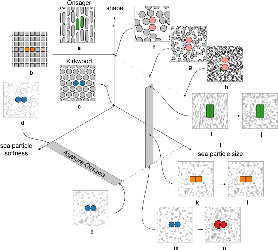
Figure 1: The general nature of entropic interactions treated in this work applies to a broad class of known systems. Here we represent them on three orthogonal axes. One axis represents, schematically, the shape of the constituent particles, with spheres at the origin. The other two axes concern the sea of particles that are being integrated out and provide the effective interaction. On one axis is the inverse of the strength of the interaction between them (where 0 represents hard steric exclusion). On the other axis is the ratio of the characteristic size of the particles of interest to that of the particle being integrated out. Other axes, not shown, represent the shape of the particle being integrated out, mixtures of particle shapes and types, etc. Examples of known experimental and model systems are sketched to illustrate their location on these axes (see references and description in text). Different coloring schemes are used to indicate penetrable sea particles , semi-penetrable sea particles , and impenetrable sea particles .

Nature is replete with shapes. In biological systems, eukaryotic cells often adopt particular shapes, for example, polyhedral erythrocytes in blood clots Cines et al. (2014), and dendritic neurons in the brain Purves et al. (2011). Before the development of genetic techniques prokaryotes were classified by shape, as bacteria of different shapes were implicated in different diseases Madigan et al. (2010). Virus capsids Mannige and Brooks (2010); Vernizzi et al. (2011) and the folded states of proteins Alberts et al. (2002) also take on well-recognized, distinct shapes. In non-living systems, recent advances in synthesis make possible granules, colloids, and nanoparticles in nearly every imaginable shape Glotzer and Solomon (2007); Tao et al. (2008); Stein et al. (2009); Sacanna and Pine (2011); Cademartiri et al. (2012); Xia et al. (2013). Even particles of nontrivial topology are now possible Senyuk et al. (2013).

The systematic study of families of idealized colloidal- and nanoscale systems by computer simulation has produced overwhelming evidence that shape is implicated in the self-assembly of model systems of particles. de Graaf et al. (2011); Damasceno et al. (2012a); Ni et al. (2012); Damasceno et al. (2012b) In these model systems, the only intrinsic forces between particles are steric, and the entropic effects of shape (which we term “shape entropy”), can be isolated. Those works show that shape entropy begins to be important when systems are at moderate density. Kamien (2007)

In laboratory systems, however, it is not possible to isolate shape entropy effects with as much control, and so the role of shape entropy in experiment is less clear. However, intuition suggests that shape entropy becomes important when packing starts to dominate intrinsic interactions, and therefore should be manifest in crowded systems in the laboratory.

Unlike other interactions, shape entropy is an emergent quantity that is expected to become important as systems become crowded. Although entropy driven phase behavior, from the crystallization of hard spheres Kirkwood (1939); Kirkwood and Monroe (1941); Kirkwood and Boggs (1942); Kirkwood et al. (1950); Alder and Wainwright (1957); Wood and Jacobson (1957), to the nematic transition in hard rods Onsager (1949), to colloid-polymer depletion interactions Asakura and Oosawa (1958), has been studied for decades, linking microscopic mechanisms with macroscopic emergent behavior is difficult in principle Anderson (1972). Hence, even for idealized systems, despite the overwhelming evidence that shape entropy is implicated in phase behavior, understanding how shape entropy is implicated is only now starting to be distilled. Frenkel (1987); Stroobants et al. (1987); Schilling et al. (2005); John et al. (2008); Triplett and Fichthorn (2008); Haji-Akbari et al. (2009, 2011a); Evers et al. (2010); Agarwal and Escobedo (2011); Zhao et al. (2011); Haji-Akbari et al. (2011b); Rossi et al. (2011); Damasceno et al. (2012a, b); Avendano and Escobedo (2012); Henzie et al. (2012); Ni et al. (2012); Zhang et al. (2012); Agarwal and Escobedo (2012); Smallenburg et al. (2012); Marechal et al. (2012, 2010); Marechal and Dijkstra (2010); de Graaf et al. (2011); Marechal and Löwen (2013); Gantapara et al. (2013); Haji-Akbari et al. (2013); Young et al. (2013, 2012); Ye et al. (2013); van Anders et al. (2014); Millan et al. (2014); Boles and Talapin (2014). For example, the phase behavior of binary hard sphere mixtures Sanders (1980); Murray and Sanders (1980); Bartlett et al. (1992); Eldridge et al. (1993); Trizac et al. (1997) or polygons Jiao et al. (2008); Zhao et al. (2011); Avendano and Escobedo (2012) can be deduced from global packing arguments, but for many other shapes,Damasceno et al. (2012b) including “simple” platonic solids like the tetrahedron Haji-Akbari et al. (2009) and its modifications,Damasceno et al. (2012a) this is not the case.

One suggestion of how shape entropy is implicated in the phase behavior of systems of anisotropic particles is through the idea of directional entropic forces (DEFs).Damasceno et al. (2012a) Damasceno et al. inferred the existence of these forces by observing that in many idealized systems of convex polyhedral shapes, one tends to observe a high degree of face-to-face alignment between particles in crystals. However, the origin and strength of these forces are unclear.

Here we use computer simulations to address how these forces arise, and construct a rigorous theoretical framework that enables this investigation. Our key results are: (i) We quantify pairwise DEFs in arbitrary systems, compute them directly in several example systems, and show they are on the order of a few $k_{\mathrm{B}}T$ just before the onset of crystallization. (ii) We show that the microscopic mechanism underlying the emergence of DEFs is the need for particles to optimize their local packing in order for the system to maximize shape entropy. (iii) By computing quantities for DEFs that can be compared to intrinsic forces between particles, we determine when shape entropy is important in laboratory systems, and suggest how to measure DEFs in the lab. (iv) We explain two notable features of the hard particle literature: the observed frequent discordance between self-assembled and densest packing structures, Haji-Akbari et al. (2011b); Damasceno et al. (2012a); Henzie et al. (2012); Damasceno et al. (2012b); Agarwal and Escobedo (2011); Haji-Akbari et al. (2013) and the high degree of correlation between particle coordination in dense fluids and crystals.Damasceno et al. (2012b) (v) As we illustrate in Fig. 1, we show that the same local dense packing mechanism that was known to drive the phase behavior of colloid-depletant systems also drives the behavior of monodisperse hard particle systems, thereby allowing us to view – within a single framework – the entropic ordering considered here and in previous works Kirkwood (1939); Kirkwood and Monroe (1941); Kirkwood and Boggs (1942); Kirkwood et al. (1950); Alder and Wainwright (1957); Wood and Jacobson (1957); Onsager (1949); Asakura and Oosawa (1958); Lekkerkerker and Tuinier (2011); Kamien (2007); Frenkel (1987); Stroobants et al. (1987); Schilling et al. (2005); John et al. (2008); Triplett and Fichthorn (2008); Haji-Akbari et al. (2009, 2011a); Evers et al. (2010); Agarwal and Escobedo (2011); Zhao et al. (2011); Haji-Akbari et al. (2011b); Rossi et al. (2011); Damasceno et al. (2012a, b); Henzie et al. (2012); Ni et al. (2012); Zhang et al. (2012); Agarwal and Escobedo (2012); Smallenburg et al. (2012); Marechal et al. (2012, 2010); Marechal and Dijkstra (2010); de Graaf et al. (2011); Marechal and Löwen (2013); Gantapara et al. (2013); Haji-Akbari et al. (2013); Young et al. (2013, 2012); Ye et al. (2013); van Anders et al. (2014); Millan et al. (2014); Boles and Talapin (2014); Mason (2002); Zhao and Mason (2007, 2008); Badaire et al. (2007, 2008); Yake et al. (2007); Snyder et al. (2009); Kraft et al. (2012); Roth et al. (2002); Odriozola et al. (2008); König et al. (2008); Sacanna et al. (2010); Odriozola and Lozada-Cassou (2013); Triplett and Fichthorn (2010); Barry and Dogic (2010).

II Methods

To compute statistical integrals we used Monte Carlo (MC) methods. For purely hard particle systems, we employed single particle move Monte Carlo (MC) simulations for both translations and rotations for systems of $1000$ particles at fixed volume. Polyhedra overlaps were checked using the GJK algorithmGilbert et al. (1988) as implemented in Damasceno et al. (2012b). For penetrable hard sphere depletant systems we computed the free volume available to the depletants using MC integration.

We quantified DEFs between anisotropic particles at arbitrary density using the potential of mean force and torque (PMFT). Such a treatment of isotropic entropic forces was first given by De Boer de Boer (1949) using the canonical potential of mean force Onsager (1933); for aspherical particles, first steps were taken in this direction in Cole (1960); Croxton and Osborn (1975).

Consider a set of arbitrary particles, not necessarily identical. Take the positions of the particles to be given by $q_{i}$, and the orientations of the particles to be given by $Q_{i}$. The partition function in the canonical ensemble, up to an overall constant, is given by

$$Z=\int[dq][dQ]e^{-\beta U(\{q\},\{Q\})}\;.$$ (1)

where $U$ is the potential energy for the interaction among the particles. Suppose that we are only interested in a single pair of particles, which we label with indices $1$ and $2$, and denote all of the other (sea) particles with a tilde. The partition function is formally an integral over all of the microstates of the system, weighted by their energies. Because we are interested in a pair of particles, we do not want to perform the whole integral to compute the partition function. Instead we break up the domain of integration into slices in which the relative position and orientation of the pair of particles is fixed; we denote this by $\Delta\xi_{12}$.

We choose to work with coordinates $\Delta\xi_{12}$ that are invariant under translating and rotating the pair of particles. In two dimensions, a pair of particles has three scalar degrees of freedom. In three dimensions, for generic particles without any continuous symmetries, a pair of particles has six scalar degrees of freedom. In the appendix A.1 we give an explicit form for these coordinates that is invariant under translations and rotations of the particle pair, and the interchange of their labels. Note that particles with continuous symmetry (i.e. spherical or axial) have fewer degrees of freedom. Separating out the integration over the sea particles gives the partition function as

$$\begin{split}Z=&\int d\Delta\xi_{12}J(\Delta\xi_{12})e^{-\beta U(\Delta\xi_{12})}\\ &\int[d\tilde{q}][d\tilde{Q}]e^{-\beta U(\{\tilde{q}\},\{\tilde{Q}\},\Delta\xi_{12})}\;.\end{split}$$ (2)

We formally integrate over the degrees of freedom of the sea particles to write

$$Z=\int d\Delta\xi_{12}J(\Delta\xi_{12})e^{-\beta U(\Delta\xi_{12})}e^{-\beta\tilde{F}_{12}(\Delta\xi_{12})}\;,$$ (3)

where $\tilde{F}_{12}$ encodes the free energy of the sea particles with the pair of interest fixed, and $J$ is the Jacobian for transforming from the absolute positions and orientations of the particles in the pair to their relative position and orientation. We define the PMFT for the particle pair $F_{12}$ implicitly through the expression

$$Z\equiv\int d\Delta\xi_{12}e^{-\beta F_{12}(\Delta\xi_{12})}\;.$$ (4)

Equating the logarithms of the integrands on the right-hand sides of Eqs. (3) and (4) gives an expression for the PMFT ($F_{12}$)

$$\begin{split}\beta F_{12}(\Delta\xi_{12})=&\beta U(\Delta\xi_{12})-\log J(\Delta\xi_{12})\\ &+\beta\tilde{F}_{12}(\Delta\xi_{12})\;.\end{split}$$ (5)

In the A.1 we outline how to extract the forces and torques from Eq. (5), and give example calculations that determine the thermally averaged equations of motion for pairs of particles.

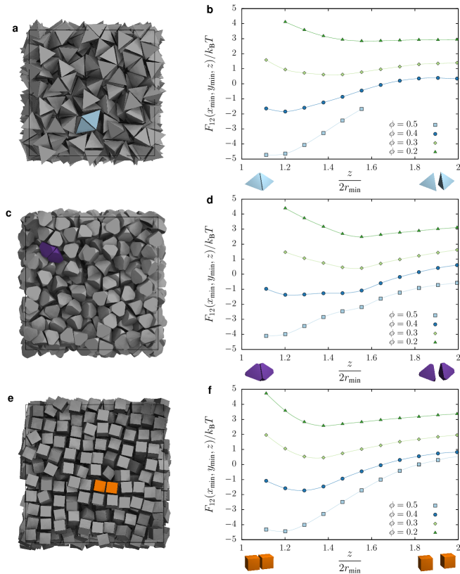
Figure 2: In monodisperse systems, we compute the PMFT by considering pairs of particles (panels a, c, and e). Density dependence of the PMFT along an axis perpendicular to the polyhedral face for a hard tetrahedra fluid (b), a fluid of tetrahedrally faceted hard spheres (d), and a hard cube fluid (f). Data are computed from the frequency histogram of the relative Cartesian coordinates of pairs of particles in MC simulations of monodisperse hard particles, and correspond to the integration of the PMFT over relative orientation. We plot along the axis that contains the global minimum of the potential, and only plot data that are within $4\;k_{\text{B}}T$ of the global minimum at each respective density, as we are able to sample such points reliably. The perpendicular distance $z$ is given in units of the minimum separation between particles, which is twice the radius of the inscribing sphere of the given polyhedron. Error bars are smaller than the markers indicating data points, and a smooth curve through the data points in each series is used to guide the eye.

In cases in which the particle pair of interest has only excluded volume interactions, as in the remainder of this paper, it is convenient to combine the first two terms to cast expression Eq. (5) as

$$\begin{split}F_{12}(\Delta\xi_{12})=&-k_{\text{B}}T\log\left(H\left(d(\Delta\xi_{12})\right)J(\Delta\xi_{12})\right)\\ &+\tilde{F}_{12}(\Delta\xi_{12})\end{split}$$ (6)

where $H$ is the Heaviside step function that we use as a bookkeeping device to ensure that the effective potential is infinite for configurations that are sterically excluded, and $d(\Delta\xi_{12})$ is the minimum separation distance of the particle pair in their relative position and orientation, which is negative when the particles overlap, and positive when they do not.

When the sea particles are penetrable hard sphere depletants, i.e. the sea particles are an ideal gas with respect to each other but hard with respect to the pair, the contribution of the sea particles to Eq. (5) can be evaluated directly. If we have $N$ penetrable hard sphere depletants, we evaluate the sea contribution $\tilde{F}_{12}(\Delta\xi_{12})$ in Eq. (5) to be

$$e^{-\beta\tilde{F}_{12}(\Delta\xi_{12})}\propto V_{\text{F}}(\Delta\xi_{12})^{N}\;,$$ (7)

where $V_{\text{F}}$ is the free volume available to the sea particles. If we consider two nearby configurations, we have that

$$\begin{split}\beta(F_{12}^{\prime}-F_{12})=&\beta(U^{\prime}-U)-N\log\left(\frac{V_{\text{F}}^{\prime}}{V_{\text{F}}}\right)\\ &-\log J^{\prime}+\log J\\ \approx&\beta(U^{\prime}-U)-\beta P(V_{\text{F}}^{\prime}-V_{\text{F}})\\ &-\log J^{\prime}+\log J\;,\end{split}$$ (8)

where we have used the ideal gas equation of state for the depletant particles. Thus, up to an irrelevant additive constant,

$$\begin{split}\beta F_{12}(\Delta\xi_{12})=&\beta U(\Delta\xi_{12})-\beta PV_{\text{F}}(\Delta\xi_{12})\\ &-\log J(\Delta\xi_{12})\;.\end{split}$$ (9)

The treatment of mixed colloid-polymer depletion systems as mutually hard colloids in the presence of non-interacting polymers is known in the literature as the penetrable hard sphere limit Lekkerkerker and Tuinier (2011). Hence Eq. (9) is the generalization of the Asakura-Oosawa Asakura and Oosawa (1958) result for depletion interactions between spherical particles to particles of arbitrary shape.

III Results

III.1 Entropic Forces in Monodisperse Hard Systems

As argued in Damasceno et al. (2012a, b) we expect that for a pair of polyhedra the DEFs favor face-to-face arrangements. In terms of the PMFT, we therefore expect face-to-face configurations to have the deepest well of effective attraction.

We compute the force components of the PMFT in Cartesian coordinates for polyhedra or polyhedrally faceted spheres and integrate over the angular directions, as described in the appendix A.2. Also, appendix B gives explicit results for torque components in an example monodisperse hard system. We then use a set of orthogonal coordinate systems for each face of the polyhedron (see Fig. 8 for a schematic diagram of this for a tetrahedron) and linearly interpolate the PMFT to the coordinate frame of each facet.

In Fig. 2 we plot the PMFT in the direction perpendicular to the face for the three systems of: (a) hard tetrahedra (b) hard tetrahedrally faceted spheres and (c) hard cubes at various densities shown in the legend. We have chosen an axis that passes through the global minimum of the potential. Several independent runs were averaged to obtain these results. Because we are free to shift the PMFT by an additive constant, we have shifted the curves for each density for clarity. We only show points that lie within $4\;k_{B}T$ of the global minimum because we can sample accurately at these points. As the density increases, the first minimum of the potential decreases, and gets closer to contact. This indicates that the particles exhibit greater alignment at higher densities as expected. Note that this is not merely an artifact of the decrease in average particle separation at higher densities because, as we show below and in appendix B, the alignment effect is concentrated near the center of the facet.

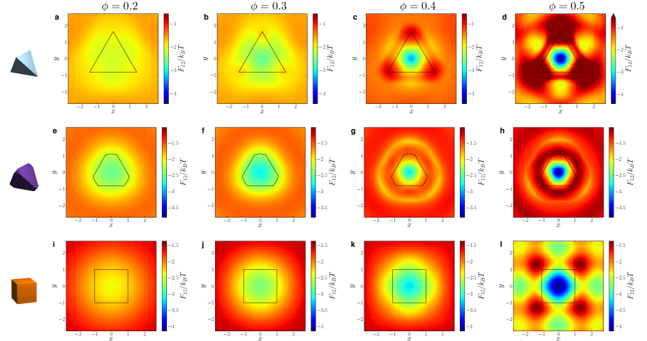
Figure 3: Directional entropic forces are emergent in systems of particles and, as such, cannot be directly imaged through microscopy. Here we show the location of potential wells by taking slices of the PMFT (computed from the frequency histogram of the relative Cartesian coordinates of pairs of particles in MC simulations of monodisperse hard particles) parallel to the faces of a tetrahedron (a-d), a tetrahedrally faceted sphere (e-h), and a cube (i-l) at various packing fractions $\phi=0.2,\,0.3,\,0.4,\,0.5$, indicated at the head of the column. As the packing fraction increases from left to right, the potential well becomes stronger, and its shape becomes more well-defined.

To understand what the PMFT is surrounding each shape we do the following. In Fig. 3 we plot the PMFT in the plane parallel to the face that passes through the global minimum of the potential (which can be identified by the minimum of the respective curve in Fig. 2). The outline of one of the faces of one particle of the pair is indicated by the solid line. The second reference particle is allowed to have its center of mass anywhere on this plane. The orientation of the second particle can vary and we integrate over all the angles. Because the particles cannot overlap, in practice not all orientations are allowed at close distances (we plot this effect for cubes in Fig. 4). Each row shows (from left to right) increasingly dense systems of tetrahedra (top row), tetrahedrally faceted spheres (middle row), and cubes (bottom row), respectively.

Directional entropic forces originate from entropic patch sites van Anders et al. (2014) – geometric features that facilitate local dense packing – but, as emergent notions, these patch sites cannot be imaged as, say, sticky patches created through gold deposition on the surface of a nanoparticle can through electron microscopy. Instead, in Fig. 3 we plot the location and strength of entropic patches at different densities. These plots show that the entropic patches lie at the centers of the facets. The effect of the pressure of the sea particles can be seen by comparing the density dependent PMFT from Eq. (6), plotted for cubes in Fig. 3i-l, to the density independent pair contribution for cubes in Fig. 4. The pair contribution clearly drives pairs of cubes away from direct face-to-face contact, and it is the other, contribution from the sea particles that is responsible for driving them together. For the polyhedral shapes, the coordination of the patches corresponds to the locations of the vertices of the dual polyhedron, and the shapes of the patches themselves at high densities appear to reflect the symmetry of the dual. In van Anders et al. (2014), we show that systematic modification of the particle shape induces DEFs between particles that lead to the self-assembly of target crystal structures.

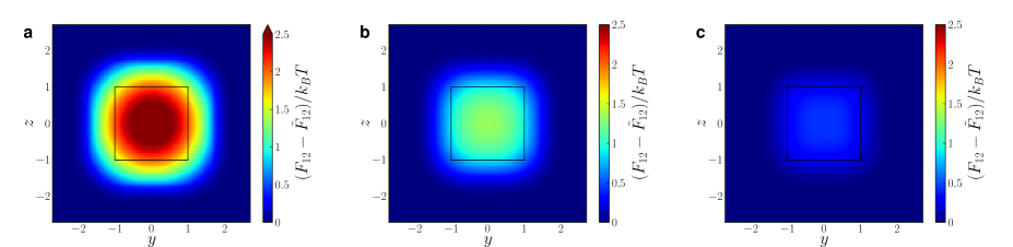
Figure 4: The density independent contribution to the PMFT for cubes at distances of $z/2r_{0}\approx 1.1$ (a), $1.2$ (b), and $1.3$ (c), which arises intrinsically from the pair of colloids under consideration, and contributes the first term factor on the right hand side in Eq. (6). This contribution provides an effective repulsion between free particles, which is stronger at small separations (a) than larger ones (b) and (c). The pattern of the repulsion is opposite that of the overall PMFT between cubes seen in Fig. 3, where both factors in Eq. (6) have been taken together.

Note that though the tetrahedron and the tetrahedrally faceted sphere share the same point group symmetry, and the geometrical coordination of basins of attraction is the same in both cases, the shape of the effective potential and its strength are different. For example, contrasting the two shapes at $\phi=0.4$ (see Fig. 3) we see that the potential difference between the center of the facet of the tetrahedrally faceted sphere and the truncated vertex is more than a $k_{\text{B}}T$ different than in the case of the actual tetrahedron. This indicates that small changes in particle shape can have dramatic effects on the structural coordination of the dense fluid.

The existence of the directionality in the PMFT in the dense fluid is strongly suggestive that DEFs provide the mechanism for crystallization. In Fig. 5 we show that DEFs persist, and increase, in the crystal. For concreteness we study systems of cubically faceted spheres that are very close to perfect cubes at a packing fraction of $\phi=0.5$ (fluid) and $\phi=0.6$ (crystal). As we show in van Anders et al. (2014), at sufficiently high packing fractions, these particles self-assemble a simple cubic lattice. Upon increasing the packing density from the fluid to the crystal, the PMFT develops stronger anisotropy. For example, by comparing the PMFT at the center of the facet to the location of the vertex of the faceting cube, we note the difference between identical points can increase by more than $1.5\;k_{\text{B}}T$.

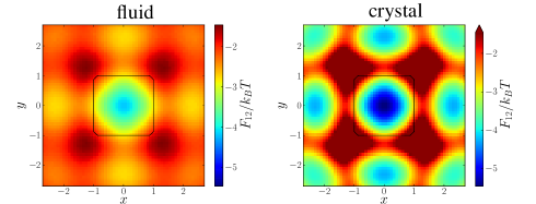
Figure 5: Directional entropic forces emerge in the fluid phase (left) and persist into the crystal (right). Here we plot the PMFT for cubically faceted spheres (from the family of shapes studied in van Anders et al. (2014)), that are nearly perfect cubes. In the dense fluid at $\phi=0.5$ (left panel) and the crystal $\phi=0.6$ (right panel) the PMFT has a similar form, but the strength of the interaction is at least $1.5\;k_{\text{B}}T$ stronger in the crystal.

III.2 Entropic Forces with Penetrable Hard Sphere Depletants

We study DEFs as a function of colloid shape in systems with traditional weakly interacting, small depletants. One system consists of a pair of spherical particles that are continuously varying faceting with a single facet, in order to promote locally dense packing. The other is a system of spherocylinders of constant radius that are continuously elongated. In each case the alteration creates a region on the surface of the particle with reduced spatial curvature.

Figure 6: The probability of specific binding, $Z_{s}$ for (a) particles with a single facet, and (b) capsules, in a bath of depletants as a function of depletant pressure. Panels (c) and (d) depict configurations that correspond to specific, semi-specific, and non-specific binding according to whether the binding occurs at sites of low curvature. Panels (e) and (f) show singly faceted spheres and spherocylinders with various facet and cylinder sizes, respectively. Curves in (a) and (b) show the probability of specific binding at various faceting amounts; with increasing patch size (more faceting) the color goes from blue to red.

As the amount of alteration to particle shape increases, it leads to stronger attraction between the sites of the reduced curvature, as encoded in the probability of observing particles with these entropic patches van Anders et al. (2014) adjacent. In the case of the faceted particle, we vary the depth of the facet linearly between zero (a sphere) and unity (a hemisphere), with the radius of the sphere fixed to $10$ (see Fig. 6e). In the case of spherocylinders, we studied cap radii fixed to $5$ and cap centers interpolating linearly between $1$ (nearly spherical) and $4$ (an elongated spherocylinder), where all lengths are in units of the depletant radius (see Fig. 6f). See appendix A.2 for computational details. In Fig. 6 a and b we show the probability that if a pair of particles is bound, then they are bound patch-to-patch entropically (specific binding) as a function of depletant pressure. Specific binding is depicted in the inset images and the left hand particle pairs in panels c and d, and is contrasted with patch-to-non-patch (semi-specific binding), and non-patch-to-non-patch (non-specific binding) in the center and right hand particle images in panels c and d. Panels a and b show that we can tune binding specificity by adjusting the patch size and the depletant pressure. Different curves correspond to increasing patch size (more faceting) as the color goes from blue to red.

For spherocylinders, it is straightforward to show the effect of the entropic patches in generating torques that cause the particles to align. To isolate the part of the torque that comes from the patch itself, we rearrange Eq. (9) for non-overlapping spherocylinders to get

$$\frac{F_{12}+k_{\text{B}}T\log J}{P\sigma^{3}}=-\frac{V_{F}}{\sigma^{3}}$$ (10)

Note that, conveniently, for ideal depletants, the expression on the right-hand side is independent of the depletant pressure. For clarity, we fix the separation distance $R$ between the spherocylinders centers of mass to be $1\%$ larger than the spherocylinder diameter (which is the minimum separation distance), and fix the orientation of each spherocylinder to be normal to the separation vector between them ($\phi_{1}=\phi_{2}=0$ in the coordinates in appendix A.1). Because it is always possible to shift the PMFT by a constant, for normalization purposes we define

$$\Omega(\chi)\equiv-\frac{V_{F}(R,\chi)}{\sigma^{3}}$$ (11)

where $\chi$ describes the angle between the spherocylinder symmetry axes. In Fig. 7 we plot $\Delta\Omega\equiv\Omega(\chi)-\Omega(0)$ for spherocylinders of different aspect ratios. For small side lengths of the spherocylinder, there is very weak dependence of the PMFT on $\chi$. As the length of the cylinder increases (and therefore as the entropic patch gets larger) the $\chi$ dependence of the PMFT becomes more pronounced. This means that not only do the particles coordinate at their entropic patch sites, but there also exists a torque Roth et al. (2002) that aligns the patches.

IV Discussion

IV.1 PMFT as an Effective Potential at Finite Density

Extracting physical mechanisms from systems that are mainly governed by entropy is, in principle, a difficult task. This difficulty arises because entropic systems have many degrees of freedom that exist at the same energy or length scale. Typically, disparities in scale are used by physicists to construct “effective” descriptions of physical systems, in which many degrees of freedom are integrated out and only the degrees of freedom key to physical mechanisms are retained. Determining which degrees of freedom are key in entropic systems is difficult because of the lack of natural hierarchies, but to extract physical mechanisms it is still necessary.

To extract the essential physics of shape for anisotropic colloidal particles, we computed the PMFT. In so doing, we described the PMFT as an effective potential, but we emphasize here that it is an effective potential in a restricted sense of the term. The restriction comes about because when we separate a system into a pair of reference colloids plus some sea particles, the sea particles can be identical to the reference colloids. Only the pair of reference colloids is described by the effective potential, which means it describes the behavior of a system of only two particles with the rest implicit. Indeed, the rest of the colloids in the system are treated as an “implicit solvent” for the pair under consideration. Because of this fact, the PMFT for monodisperse colloids is not synonymous with the bare interaction potential for the whole system. Note that in systems of multiple species, there is some possibility of a broader interpretation of the PMFT for a single species having integrated out another species Dijkstra et al. (1999), but even in that case, difficulties arise.Louis (2002) E.g., Onsager treated the nematic transition in hard rods by considering rods of different orientations as different “species” Onsager (1949), but an effective potential between rods of the same “species” or orientation does not capture the physics of the system in the same way that an effective potential between rods induced by polymer depletants would.Kamien (2007)

Interpreting the PMFT from Eq. (5) in the restricted sense, we see that it naturally exhibits three contributions. (i) The first term on the right hand side is the bare interaction between the pair of particles, which originates from van der Waals, electrostatic, or other interactions of the system of interest. It encodes the preference for a pair of particles to be in a particular relative position and orientation. Here, we are mostly concerned with hard particles, so this term encodes the excluded volume interaction. (ii) The second term on the right hand side is the logarithmic contribution from the Jacobian; it counts the relative number of ways that the pair of particles can exist in a relative position and orientation. For a more technical discussion of this term, see appendix C. (iii) The third term is the free energy of the sea particles that are integrated out, keeping the relative position and orientation of the pair fixed. In purely hard systems this last term is sea particle entropy, which is just the logarithm of the number of microstates available to the sea particles for that configuration of the pair.

The free energy minimizing configuration of the pair of particles is determined by a competition between the three terms in Eq. (5). Consider the contribution from the third term. For any non-attractive bare interactions between sea particles, if the pair of particles is separated by a distance that is less than the effective diameter of the sea particlesMalescio and Pellicane (2003), and adopts a configuration that packs more densely, the free energy of the sea particles will never increase. This is the case for bare interactions that are repulsive due to excluded volume (in which case the system is dominated by entropy) and for sea particles that are soft and interpenetrable.

In the absence of the first two terms in Eq. (5), the third term will drive the pair of particles into denser local packing configurations. The driving force for local dense packing becomes stronger as the system density increases. To understand why this occurs, we note that DEFs arise by the pair of particles balancing the pressure of the sea particles. Rather than considering the effects of the sea on the pair, we will momentarily consider the effects of the pair on the sea. The pair of interest forms part of the ‘box’ for the sea particles. Density dependence arises because changes in the relative position and orientation are related to the local stress tensor. This contribution is on the order of $P\sigma^{3}/k_{\mathrm{B}}T$, where $P$ is the characteristic scale of the local stress tensor, which we expect to be related to the pressure, and $\sigma$ is a characteristic length scale. Since this contribution is density dependent the effective forces between particles are emergent. These emergent forces are directional, because some local packing configurations are preferred over others. For example, dense local packing configurations involve face-to-face contact for many particles, which is why face-to-face contact is observed in so many hard-particle crystals, and is borne out in Fig. 3. This is also, of course, akin hard rods aligning axes in nematic liquid crystalsOnsager (1949). Indeed, in repulsive systems, only at sufficiently high densities is the system able to overcome any repulsion from the first two terms in Eq. (5), plotted in Fig. 4 for cubes, which drive the system away from locally dense packings. It is this competition between the drive towards local dense packing supplied by the sea particles’ entropy, and the preferred local relative positions and orientations of the pair, which is induced by the maximization of shape entropy, that determines the self-assembly of entropic systems of repulsive (hard) shapes.

Two general lessons from the literature of hard particle self-assembly are intuitive in light of the mechanism we have described.

First, in a previous systematic study of shape and self-assembly using a family of highly symmetric convex polyhedra,Damasceno et al. (2012b) it was shown that there is a remarkable correlation between the number of nearest neighbors in the crystal structure of a given polyhedron, and the number of nearest neighbors in the dense fluid. Since systems at finite density exhibit a drive towards local dense packing, we would expect that the organization of neighbor shells to be determined by the same local packing considerations in both the dense fluid and the crystal. Indeed, we might expect to predict crystal structure based on local packing considerations alone. In recent work we designed particle shape to favor certain local dense packing arrangements to self-assemble targeted crystal structures.van Anders et al. (2014) We viewed the induced anisotropy of the effective interactions between particles as the entropic analogue of the intrinsic anisotropic interactions between enthalpically patchy particlesZhang and Glotzer (2004); Glotzer and Solomon (2007). Attractive entropic patches are features in particle shape that facilitate local dense packing.

Second, hard particle systems often assemble into their densest packing structure, however some do not Haji-Akbari et al. (2011b); Damasceno et al. (2012a); Henzie et al. (2012); Damasceno et al. (2012b); Agarwal and Escobedo (2011); Haji-Akbari et al. (2013). The present work helps to highlight two key differences between self-assembly and packing. (i) Systems self-assemble because the second law of thermodynamics drives them free energy minima, so like packing, self-assembly has a mathematical optimization problem at its root. In assembling systems, all three terms in Eq. (5) contribute, but in the infinite pressure limit relevant for packing, the entropy of the pair of particles does not contribute. This is because the first term provides the steric hindrance between particles, and the third term should scale with pressure, whereas the second term encodes the entropy of a set of relative positions and orientations of the pair, and this factor becomes irrelevant in the infinite pressure limit. (ii) Assembly is related to local dense packing, that we have characterized here with two-body potentials, whereas global dense packing is ostensibly an “all-body problem.” Given these two differences it might be more surprising that densest packing solutions ever coincide with assembled structures, than the fact that they frequently do not. However, the pair entropy term often only separates particles, while preserving their alignment, e.g. we showed particles are more frequently observed with face-to-face alignment at small separations, than in direct face-to-face contact. Moreover, in practice (e.g. Chen et al. (2014)), the solution to the all-body packing problem is often given by the solution to a few-body problem.

Figure 7: The angular ($\chi$) dependence of the portion of the PMFT directly attributable to modification of particle shape ($\Omega$, see Eq. (11), normalized to $0$ at $\chi=0$) for spherocylinders in the presence of penetrable hard sphere depletants for different cylinder side lengths. For short side length ($\ell=1$, light blue squares) there is very little angular variation indicating very little entropic torque. As the side length, $\ell$, increases from to $5$ (in units of the depletant radius, pink triangles), the strength of the dependence on $\chi$ increases, indicating greater torques, as expected.

IV.2 Unification

We have seen above that directional entropic forces, as captured by the PMFT, arise when particles maximize shape entropy through local dense packing. We verified this drive to local dense packing with direct calculations for monodisperse hard shapes, and for hard shapes in a sea of penetrable hard sphere depletants. Monodisperse hard-particle systems and colloid-depletant systems would, at first glance, seem to be different.

However, depletion systemsAsakura and Oosawa (1958) and monodisperse systems of hard anisotropic shapes are both entropy-driven, as is the crystallization of hard spheres,Kirkwood (1939); Kirkwood and Monroe (1941); Kirkwood and Boggs (1942); Kirkwood et al. (1950); Alder and Wainwright (1957); Wood and Jacobson (1957) and the nematic liquid crystal transition in hard rods Onsager (1949). Indeed, since original work by Asakura and Oosawa Asakura and Oosawa (1958) on depletion interactions, it has been well known that the depletion-induced aggregation of colloids arises from an osmotic effect in which depletants liberate free volume for themselves by driving the colloids into dense packing configurations. However, earlier work of de Boer de Boer (1949) suggested that considerations of the potential of mean force in systems of isotropic particles leads to pairs of particles having certain preferred distances because they balance their own repulsive forces with the sea particles’ preference for them to pack more densely.

In traditional depletion systems, the depletants are small compared with the colloids, spherical, and interpenetrable. In such systems, there is a substantial literature on the anisotropic binding of colloids by depletants starting with Mason (2002), and followed by work on rough colloids Zhao and Mason (2007, 2008); Badaire et al. (2007, 2008); Yake et al. (2007); Snyder et al. (2009); Kraft et al. (2012), as well as more anisotropic shapes Roth et al. (2002); Triplett and Fichthorn (2010); Rossi et al. (2011); Young et al. (2012); Barry and Dogic (2010), and lock-and-key systems Odriozola et al. (2008); König et al. (2008); Sacanna et al. (2010); Odriozola and Lozada-Cassou (2013). In all of these systems, the anisotropic binding can be seen as resulting from a sea of depletants forcing colloids to adopt local dense packing configurations.

However, one might ask how large, or hard, or aspherical can the depletants be, before they cease to act as depletants? In the original work of Asakura and Oosawa Asakura and Oosawa (1958), depletants were not restricted to be small; large depletants are the so-called “protein limit”Lekkerkerker and Tuinier (2011). In experimental systems, and accurate models, depletants are not freely interpenetrable. Baumgartl et al. (2007); Dijkstra et al. (1999); Lekkerkerker and Tuinier (2011) In the original work of Asakura and Oosawa Asakura and Oosawa (1958), depletants were imagined to be polymers, which are certainly not spherical, but were modelled as spheres.

The fact that depletants can be aspherical, or hard, or large, is of course well-known; in all cases depletants exert an osmotic pressure that causes colloids to aggregate, as the colloids adopt dense packing configurations. However, we argued above that consideration of the three contributions to the PMFT in Eq. (5) leads to a drive towards local dense packing in generic systems in which the sea particles can be simultaneously arbitrarily aspherical, hard, and large. Indeed the sea particles can be the same species as the colloids, and still behave as “depletants”. Hence the classic works on the entropic behavior of systems as diverse as hard shapes from spheresKirkwood (1939); Kirkwood and Monroe (1941); Kirkwood and Boggs (1942); Kirkwood et al. (1950); Alder and Wainwright (1957); Wood and Jacobson (1957), to rodsOnsager (1949), to tetrahedraHaji-Akbari et al. (2009), and colloid-depletant systemsAsakura and Oosawa (1958); Lekkerkerker and Tuinier (2011) are not similar only because their phase behavior is driven by entropy. In addition, they are similar because entropy controls their phase behavior through a preference for local dense packing.

In Fig. 1 we showed a schematic representation of the family of systems whose phase behavior is governed by the shape-entropy driven mechanism. We represent the family of systems on a set of three axes. One axis represents the shape of the colloidal pair of interest, in which we think of spheres as occupying the “zero” limit and rods infinity. A second axis is the softness of the sea particles; one limit represents hard-core particles (vanishing softness) and the other an interpenetrable ideal gas (for spherical sea particles, in the case that the sea particles can be considered as depletants, this is the so-called penetrable hard sphere limit Lekkerkerker and Tuinier (2011)). A third axis is the inverse size of the sea particles, where a monodisperse system is at the origin, and the other limit has sea particles being very small compared to the “colloids”. One could also include other axes, such as the shape of the sea particles, or the density of the system, but we omit them for simplicity.

As a guide we have indicated the location of some well-studied model and experimental systems on these axes. Hard spheres sit at the origin (c),Kirkwood (1939); Kirkwood and Monroe (1941); Kirkwood and Boggs (1942); Kirkwood et al. (1950); Alder and Wainwright (1957); Wood and Jacobson (1957) hard rodsOnsager (1949) lie at the extreme of the shape axis (a), and Asakura and Oosawa’s model of depletantsAsakura and Oosawa (1958) lies in the plane of zero shape (between d and e). Some depletion systems are indicated (i,k,m); however in experiments, particles are not all of the same shape, and are sometimes actually binary (j,l) or ternary (n) mixtures. Monodisperse hard particle systems lie along the shape axis (b,f), but are simply a limit of binary hard systems (g,h).

IV.3 DEFs in Experimental Systems

We have shown that DEFs arise from a mechanism that occurs in a wide variety of idealized systems. Do DEFs and shape entropy matter for experimental systems? Using systems in which shape entropy is the only factor that determines behavior, we have shown that in several example systems DEFs are on the order of a few $k_{\mathrm{B}}T$ around the onset of crystallization. This puts DEFs directly in the relevant range for experimental systems. If in experiment there is sufficient control over the intrinsic forces between colloids that puts them at much less than the $k_{\mathrm{B}}T$ scale, systems will be shape entropy dominated. If the intrinsic forces are on the order of a $k_{\mathrm{B}}T$, then there will be a competition between directional entropic forces and intrinsic forces. If the scale of the intrinsic forces are much more than a few $k_{\mathrm{B}}T$, intrinsic forces will dominate shape entropy effects.

Can these forces be measured in the laboratory? In colloidal experiments, effective interaction potentials can be inferred from the trajectories of the colloids in situ, e.g. by confocal microscopy Iacovella et al. (2010). Recently, it has become possible to image anisotropic colloids in confocal microscopes and extract particle positions and orientations.Mohraz and Solomon (2005); Shah et al. (2013) The determination of both particle positions and orientations makes it possible to directly extract the PMFTs computed here from experimental data. For isotropic potentials of mean force, this investigation has already been carried out by analyzing the pair correlation function $g(r)$.Iacovella et al. (2010) As in Iacovella et al. (2010), we can interpret this potential measurement as describing the thermally averaged time evolution of the relative position and orientation of pairs of particles. Furthermore, we have shown that pairs of particles are described by the PMFT regardless of the properties of the sea particles, so the PMFT describes the average time evolution of pairs of particles in monodisperse systems, as well as colloid-depletant systems.

V Conclusions

In this paper we showed that shape entropy drives the phase behavior of systems of anisotropic shapes through directional entropic forces. We defined DEFs in arbitrary systems and showed that they are emergent, and on the order of a few $k_{\mathrm{B}}T$ just below the onset of crystallization in example hard particle systems. By quantifying DEFs we put the effective forces arising from shape entropy on the same footing as intrinsic forces between particles that are important for self-assembly. In nano- and colloidal systems our results show that shape entropy plays a role in phase behavior when intrinsic forces between particles are on the order of a few $k_{\mathrm{B}}T$ or less. This figure guides the degree of control of intrinsic forces in particle synthesis required for controlling shape entropy effects in experiment. In microbiological systems it facilitates the comparison of the effects of rigid shape in crowded environments with the elasticity of the constituents. We suggested how existing experimental techniques could be used to measure these forces directly in the laboratory. We showed that the mechanism that generates DEFs is that maximizing shape entropy drives particles to adopt local dense packing configurations.

Finally, we demonstrated that shape entropy drives the emergence of DEFs, as particles adopt local dense packing configurations, in a wide class of soft matter systems. This shows that in a wide class of systems with entropy driven phase behavior, entropy drives the phase behavior through the same mechanism Kirkwood (1939); Kirkwood and Monroe (1941); Kirkwood and Boggs (1942); Kirkwood et al. (1950); Alder and Wainwright (1957); Wood and Jacobson (1957); Onsager (1949); Asakura and Oosawa (1958).

Appendix A Supplementary Methods

A.1 Further Analytical Considerations

A.1.1 Jacobian Factor

We have included the Jacobian factor in our definition of the PMFT. The motivation for doing this is that by explicitly including this term we do not want to either ignore or introduce any artifacts that might stem from a poor choice of coordinates for a given problem. Note that for general particles in three dimensions, the PMFT is defined on the space $\mathbb{R}^{3}\times\mathbb{RP}^{3}$. This means that even if the pair interaction is purely hard, whenever there is non-trivial shape, some relative pair configurations are preferred over others. In standard treatments of the isotropic potential of mean force, it is not conventional to include the Jacobian factor. The choice not to include it in that case is well-motivated by the existence of a single “natural” coordinate system in that case that prevents any ambiguity there. In either case, one must take account of the inclusion or not of this factor in writing down the effective equations of motion for the pair.

A.1.2 Axisymmetric Coordinate System for PMFT

We present an explicit computation of the Jacobian of the change of variables between the natural coordinates of a pair of particles, and the scalar invariant quantities that describe any such pair. We do so in the simpler case of axisymmetric particles. The general case can be computed straightforwardly in the same manner, but the expressions are cumbersome.

We take the first particle to be at the origin, with its symmetry axis oriented in the positive $z$ direction. Using the azimuthal symmetry with this placement, we fix the second particle’s position in the $xy$-plane, without loss of generality to be along the $x$ axis. This gives the orientation of the second particle as

$$\hat{n}_{2}=\sin\theta\cos\varphi\hat{x}+\sin\theta\sin\varphi\hat{y}+\cos\theta\hat{z}$$ (12)

where $\theta$ and $\varphi$ are spherical coordinates in the coordinate system of the second particle, and its position as

$$r_{2}-r_{1}=\rho\hat{x}+z\hat{z}$$ (13)

where $\rho$ and $z$ are cylindrical coordinates in the first particle’s coordinate system. The volume form that appears in the integral that computes the partition function is

$$dV=\rho\sin\theta d\rho dzd\theta d\varphi$$ (14)

Now we make the change of variables to the scalar invariant quantities by taking

$$\begin{split}R&=\sqrt{z^{2}+\rho^{2}}\\ \phi_{1}&=\frac{z}{\sqrt{z^{2}+\rho^{2}}}\\ \phi_{2}&=-\frac{\rho\sin\theta\cos\varphi+z\cos\theta}{\sqrt{z^{2}+\rho^{2}}}\\ \chi&=-\cos\theta\end{split}$$ (15)

Inverting the relationship between the two coordinate systems gives

$$\begin{split}\rho&=R\sqrt{1-\phi_{1}^{2}}\\ z&=R\phi_{1}\\ \theta&=-\cos^{-1}\chi\\ \varphi&=\cos^{-1}\left(\frac{-\phi_{1}\chi-\phi_{2}}{\sqrt{(1-\chi^{2})(1-\phi_{1}^{2})}}\right)\end{split}$$ (16)

The computation of the determinant is simplified by noting the dependence of $\rho$ and $z$ on only $R$ and $\phi_{1}$, and $\theta$ on only $\chi$. This means that we only need to consider the dependence of $\varphi$ on $\phi_{2}$. Taking the determinant of this leads to the new volume form

$$dV=\frac{R^{2}dRd\phi_{1}d\phi_{2}d\chi}{\sqrt{1-\chi^{2}-\phi_{1}^{2}-\phi_{2}^{2}-2\phi_{1}\phi_{2}\chi}}$$ (17)

In the absence of the excluded volume (or other) interaction between the particles, this expression measures the volume of configuration space available to a pair of free particles in a particular translationally and rotationally invariant configuration.

To verify that our expression correctly encodes the density of states for two free axisymmetric particles, we consider the following scenario. Suppose we had a pair of axisymmetric particles each undergoing Brownian motion with the constraint that their centers of mass could never be separated by a distance greater than $R_{\text{max}}$, but that they were otherwise free to move, including to interpenetrate. If we were to make some $N_{\text{obs}}$ uncorrelated observations of the particles for each of which we determine the values of $R$, $\phi_{1}$, $\phi_{2}$, and $\chi$, we would find that their frequency distribution would converge to something proportional to the Jacobian of our coordinate transformation in the limit that $N_{\text{obs}}\to\infty$. We therefore verified our expression by performing precisely this calculation.

A.1.3 General Coordinate System for PMFT

For the general case in three dimensions, a pair of particle has six degrees of freedom that are invariant under global translations and rotations. Let us take the particles to be situated at $\vec{x}_{1,2}$, and have orientations $\mathbf{q}_{1,2}$. Starting with the positions, the separation of the particles in position space is simply given by the vector $\vec{r}_{12}=\vec{x}_{2}-\vec{x}_{1}$. This gives a set of coordinates that are invariant under translations, but not under rotations. We therefore seek to form six scalars by taking combinations of this vector with the particle orientations.

To treat the particle orientations on a similar footing to the positions, we need to determine the separation in orientation of the particles. We note that that each of the particle orientations is given by an element of $SO(3)$, the rotation group in three dimensions. While it is possible to work with this group directly, the calculations that follow can be simplified greatly by noting that $SU(2)$ is the double cover of $SO(3)$, and working with $SU(2)$ instead. For concreteness, we will use the conventions common in quantum mechanics and write our particle orientations as rotation operators according to

$$\mathbf{q}_{i}=e^{i\frac{\theta_{i}}{2}\hat{n}\cdot\vec{\sigma}}\;,$$ (18)

where $\theta_{i}$ is the angle of rotation $\hat{n}_{i}$ is the normal to the plane of the rotation and $\vec{\sigma}$ are the Pauli matrices. From this form it is clear that under a global rotation, the particle orientations transform in the reducible representation expressed in Young tableaux as

$$\yng(1)\otimes\yng(1)=\yng(1,1)\oplus\yng(2)\;.$$ (19)

This can be understood intuitively in the following way: if you rotate a particle by some amount in some plane, two different observers will agree on the amount of the rotation, but will give the normal to the plane in their own coordinates. The amount of the rotation is the scalar $\yng(1,1)$, and the normal to the plane is the vector $\yng(2)$. In a similar fashion to the way in which we combined particle positions to yield a relative position, we will combine particle orientations. A Clebsh-Gordan decomposition of the particle orientations gives

$$\begin{split}\left(\yng(1)\otimes\yng(1)\right)\otimes\left(\yng(1)\otimes\yng(1)\right)=\;&\yng(2,2)\oplus\yng(2,2)\\ &\oplus\yng(3,1)\oplus\yng(3,1)\oplus\yng(3,1)\\ &\oplus\yng(4)\;,\end{split}$$ (20)

which means that the combination of the two orientations yields two scalars (spin 0), three vectors (spin 1), and a tensor (spin 2).

For convenience, we note that the spin 1 representation of $SU(2)$ $\yng(2)$ is also the adjoint representation of $SU(2)$. This means that we can write vectors in ordinary space by using the Pauli matrices as Cartesian unit vectors according to

$$\vec{v}=\sum_{i}\vec{v}\cdot\hat{e}_{i}\sigma_{i}\;.$$ (21)

In this representation, if we combine orientations expressed in terms of Pauli matrices as in (18), products of orientations that are proportional to the identity matrix are scalar quantities, and products that are not are vectors. We will use this fact momentarily.

For the purposes of creating scalar invariants by combining them among themselves, and with the particle separation in position, the scalars and vectors that arise from combining orientations are of interest. We determine these scalars and vectors explicitly by taking symmetrized Hermitian products of the particle orientations. We find the scalars can be expressed as

$$\begin{split}S_{12}=&\frac{1}{2}(\mathbf{q}_{1}\mathbf{q}_{2}^{\dagger}+\mathbf{q}_{2}\mathbf{q}_{1}^{\dagger})\\ U_{12}=&\frac{1}{4}(\mathbf{q}_{1}\mathbf{q}_{2}+\mathbf{q}_{2}\mathbf{q}_{1}+\mathbf{q}_{1}^{\dagger}\mathbf{q}_{2}^{\dagger}+\mathbf{q}_{2}^{\dagger}\mathbf{q}_{1}^{\dagger})\end{split}$$ (22)

and the vectors as

$$\begin{split}V_{12}=&\frac{i}{4}(\mathbf{q}_{1}\mathbf{q}_{2}-\mathbf{q}_{2}\mathbf{q}_{1}+\mathbf{q}_{1}^{\dagger}\mathbf{q}_{2}^{\dagger}-\mathbf{q}_{2}^{\dagger}\mathbf{q}_{1}^{\dagger})\\ W_{12}=&-\frac{i}{4}(\mathbf{q}_{1}\mathbf{q}_{2}+\mathbf{q}_{2}\mathbf{q}_{1}-\mathbf{q}_{1}^{\dagger}\mathbf{q}_{2}^{\dagger}-\mathbf{q}_{2}^{\dagger}\mathbf{q}_{1}^{\dagger})\\ T_{12}=&-\frac{i}{2}(\mathbf{q}_{1}\mathbf{q}_{2}^{\dagger}-\mathbf{q}_{2}\mathbf{q}_{1}^{\dagger})-V_{12}\\ \end{split}$$ (23)

which we have identified according to their matrix form. Using our convention for representing the particle orientations we find

$$\begin{split}S_{12}=&\cos\left(\frac{\theta_{1}-\theta_{2}}{2}\right)\\ U_{12}=&\cos\left(\frac{\theta_{1}+\theta_{2}}{2}\right)\\ V_{12}=&\frac{1}{2}(\hat{n}_{1}\times\hat{n}_{2})(S_{12}-U_{12})\\ W_{12}=&\sin\left(\frac{\theta_{1}+\theta_{2}}{2}\right)\frac{\hat{n}_{1}+\hat{n}_{2}}{2}+\sin\left(\frac{\theta_{1}-\theta_{2}}{2}\right)\frac{\hat{n}_{1}-\hat{n}_{2}}{2}\\ T_{12}=&\sin\left(\frac{\theta_{1}+\theta_{2}}{2}\right)\frac{\hat{n}_{1}+\hat{n}_{2}}{2}-\sin\left(\frac{\theta_{1}-\theta_{2}}{2}\right)\frac{\hat{n}_{1}-\hat{n}_{2}}{2}\end{split}$$ (24)

By combining these quantities with $\vec{r}_{12}$ we can form the six scalar invariants

$$\{|\vec{r}_{12}|,\;S_{12},\;U_{12},\;\hat{r}_{12}\cdot W_{12},\;\hat{r}_{12}\cdot V_{12},\;W_{12}\cdot T_{12}\}$$ (25)

For the purposes of showing the coordination of particles in space at the location of faces or facets, it is convenient to integrate over some of the angular degrees of freedom, and to work in Cartesian coordinates. In particular, it is very convenient to work in Cartesian coordinates adapted to the particle facets as shown in Fig. 8 for tetrahedral facets.

A.1.4 Forces and Torques

For concreteness, we give an example for how to compute the forces and torques from the PMFT. As usual, forces and torques arise from taking the negative gradient of the potential. For force components this is straightfoward. For torques, we give an explicit expression for the case of axisymmetric particles.

To compute the torques, we continue to work in terms of rotation matrices in the spin $\frac{1}{2}$ representation of $SU(2)$. If $\mathbf{q}$ is the rotation, then to determine the torque, we must differentiate the PMFT with respect to it. If we represent the rotations in the canonical fashion, and use Pauli matrices as the basis vectors of the Cartesian space coordinates, then we have scalar products of the form

$$\vec{a}\cdot\vec{b}=\frac{1}{2}\operatorname{Tr}(a^{\dagger}b)$$ (26)

and cross products of the form

$$\vec{a}\times\vec{b}=\frac{1}{2i}[a,b]$$ (27)

Our potential depends on scalar products alone. That means to determine the torque we are required to know, e.g., that if

$$\phi_{1}=\frac{1}{2}\operatorname{Tr}(\mathbf{q}^{\dagger}\hat{z}\mathbf{q}\hat{r}_{12})$$ (28)

then

$$\frac{\partial\phi_{1}}{\partial\mathbf{q}}=\frac{1}{2}\mathbf{q}^{\dagger}\left[\mathbf{q}\hat{r}_{12}\mathbf{q}^{\dagger},\hat{z}\right]$$ (29)

which we recognize as a cross product. We have taken, without loss of generality, the reference vector to be $\hat{z}$ in the coordinate frame of the particle. We then use the chain rule to differentiate $F_{12}$ with respect to $\mathbf{q}$, and convert back to Cartesian coordinates to find a contribution to the torque of the form

$$\vec{T}_{\phi_{1}}=-\hat{r}_{12}\times\hat{n}_{1}\frac{\partial F_{12}}{\partial\phi_{1}}$$ (30)

Similar manipulations yield the other contributions.

A.2 Numerical Methods

A.2.1 Monodisperse Systems

For hard particle systems, the various contributions in Eq. (5) (main text) can be computed using different means. The pair interaction term ($\beta U$) is given by the pair overlap function, which is known, at least in principle. The pair Jacobian term ($-\log J$) can be computed analytically, as we describe below. The third contribution ($\beta\tilde{F}_{12}$) could be computed by determining the free energy of the rest of the system for a series of fixed configurations of the pair. In practice, we are not interested in the contributions of each of the individual terms per se, so instead we compute their sum directly. We obtain the PMFT on the left hand side of Eq. (5) (main text) by computing the frequency histogram of the relative pair coordinates and orientations, and taking its logarithm, as suggested by the form of Eq. (4) (main text). This gives the PMFT up to an overall irrelevant additive constant.

Since the PMFT is a generalization of the potential of mean force, the method for computing the PMFT is a straightforward generalization of the method used to extract the potential of mean force from the radial distribution function $g(r)$. In detail, over the course of a MC simulation trajectory, we measure all of the relative positions of each pair of particles that fall within a given cutoff distance (for the results we present in the main text we integrate over the relative orientations). We impose a discrete grid over the set of allowed relative positions, and record the number of pairs that fall within each grid cell. This tabulation of the relative frequency of the various configurations, gives us a measurement of the $g(x,y,z)$ analogue of $g(r)$, and so simply taking the logarithm gives us $F_{12}$ from Eq. (5) (main text).

Computing the PMFT in this manner introduces two forms of systematic discretization error. To illustrate the sources of this error we will give a more detailed description of the calculation we performed. We wish to compute the PMFT at some given relative position and orientation. For concreteness, and to keep formulae simple, let us consider just computing the force component. In principle, one can compute the PMFT by performing thermodynamic integration or umbrella sampling over various fixed relative particle positions if one wants the exact potential difference between particular relative pair positions and orientations. However, in our case we are interested in the general geometric features of the potential, for which it is sufficient to perform simulations in a standard ensemble, and record the relative frequency of various events. Thus we compute an approximate value, $F^{\prime}_{12}$, of the true PMFT, $F_{12}$, at some point $(x_{i},y_{i},z_{i})$ by averaging over a bin of size $(\Delta x,\Delta y,\Delta z)$ centered at that point according to

$$\Delta x\Delta y\Delta ze^{-\beta F^{\prime}_{12}(x_{i},y_{i},z_{i})}\equiv\int_{\text{bin}_{i}}dxdydze^{-\beta F_{12}(x,y,z)}\;.$$ (31)

If the true potential of mean force and torque is slowly varying over the bin, in the sense that

$$\begin{split}\left|\int_{\text{bin}_{i}}dxdydz(\vec{x}-\vec{x}_{i})\cdot\nabla\left.e^{-\beta F_{12}(x,y,z)}\right|_{\vec{x}=\vec{x}_{i}}\right|\\ \ll\Delta x\Delta y\Delta ze^{-\beta F_{12}(x_{i},y_{i},z_{i})}\;,\end{split}$$ (32)

then we can Taylor expand the integrand about $(x_{i},y_{i},z_{i})$, and, assuming that the whole bin is allowed, we find that

$$\Delta x\Delta y\Delta ze^{-\beta F^{\prime}_{12}(x_{i},y_{i},z_{i})}\approx\Delta x\Delta y\Delta ze^{-\beta F_{12}(x_{i},y_{i},z_{i})}\;.$$ (33)

This gives $F^{\prime}_{12}(x_{i},y_{i},z_{i})\approx F_{12}(x_{i},y_{i},z_{i})$. This approximation breaks down if $F_{12}$ is not sufficiently slowly varying, in the above sense. It also breaks down if the bin is partially forbidden, i.e. if the integrating volume is not $\Delta x\Delta y\Delta z$. We expect the PMFT to vary quickly at the boundaries of regions that are forbidden due to overlap, i.e. we expect the effective potential to be relatively “hard”. This means that at the edges of these regions, where we would have difficulty sampling events, we would also expect to have to resolve minute differences to obtain meaningful results. This makes such a technique prohibitively difficult for such boundary cases where one would have to resort to umbrella sampling. As a result (in particular in Figs. 2, 3, and 5, main text) we only show the PMFT for points that are within $4\;k_{\text{B}}T$ of the global minimum, because it is at these points that we can sample the potential reliably in the sense described above, using our method.

A.2.2 Penetrable Hard Sphere Systems

Here we explain how we calculate the PMFT for a pair of hard, arbitrarily shaped colloidal particles in a sea of smaller penetrable hard sphere depletants.

As we showed in Eq. (9) (main text), the PMFT takes on a simplified form in the case of penetrable hard sphere depletants and thus the contribution from integrating out the depletants $\tilde{F}_{12}$ can be computed more easily. The contribution from the colloid pair potential is, in principle, known, as before, and the Jacobian can be computed as described below. The problem is therefore reduced to computing the contribution that comes from the free volume available to the depletants for a fixed configuration of the colloidal pair.

We computed the free volume in the penetrable hard sphere model of depletants by MC integration. The same results could also be obtained by direct MC simulations with explicit ideal depletants, as discussed below, or by some other numerical integration method. To accelerate this computation, we make note of the following. The change in free volume between a given configuration and widely separated particles falls entirely within the intersection of two spheres, each enclosing a particle. The volume of this region of intersection is smallest (and, therefore, computation is most efficient) if the radii of the spheres in question are as small as possible. This is given by having a sphere enclosing each particle with a radius given by the sum of the radius of a sphere that circumscribes the particle and the radius of a sphere that circumscribes the depletant.

For a given relative position and orientation of the colloids, we computed the intersection of spheres that determined this region and computed the change in free volume by throwing random depletants uniformly over the region and computing the fraction that intersected both colloids. We performed five independent runs for each system. We used 500 MC integration points per unit volume of the region of intersection, and 1000 total throws if the volume of intersection was less than one unit. This fraction of the total volume gives the change in free volume available to the depletants. In the case of faceted spheres, overlap checks between particles were performed by casting the overlap as an optimization problem that we solved using the Karush-Kuhn-Tucker method Ruszczyński, Andrzej (2006). In the case of spherocylinders, the Bullet physics library Coumans (2012) was used to check overlaps.

As noted above, the Jacobian of the transformation to invariant coordinates can be computed analytically, which we did. We checked our analytical calculation numerically by performing a MC simulation of a pair of free axisymmetric particles. The frequency histogram of the occurrence of the invariant coordinates was checked against the analytic form and found to match.

To examine these systems in detail it is convenient to use the language of entropic patches from van Anders et al. (2014). We define the probability of specific binding at a pair of entropic patch sites as the probability of finding a pair of particles at the set of configurations that are in the basin of attraction of perfect alignment. We obtain this by integrating the Boltzmann weight over the set of configurations.

For concreteness, consider a pair of hemispherical particles in a bath of depletants. The probability of specific binding can be cast formally as the integral

$$\begin{split}Z_{s}\propto&\int_{0}^{1}d\phi_{1}\int_{0}^{1}d\phi_{2}\int dRd\chi e^{-\beta F_{12}(R,\phi_{1},\phi_{2},\chi)}H(-\beta P\Delta V_{\text{F}})\;.\end{split}$$ (34)

The upper bounds on the $\phi$ integrals correspond to coincident faces. The step $H$ function ensures that we are only integrating over configurations in which there is entropic binding. Similar integrals can be defined for semi-specific binding (patch to non-patch) and non-specific binding (non-patch to non-patch).

Figure 8: An illustration of the choice of four sets of orthogonal coordinates for each of the faces of a tetrahedron, which we use for subsequent computations in Figs. 2 and 3 (main text). The face normals, which we take to be the $z$ coordinates in the frame of the face are shown in blue. Similarly, the $x$ and $y$ coordinates in the frame of the face are shown in green and red respectively.

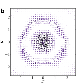
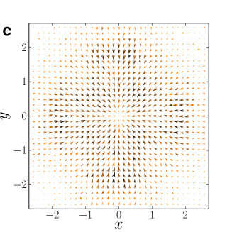
Figure 9: DEFs in Cartesian coordinates for monodisperse hard particle systems at a packing fraction of $\eta=0.4$ for tetrahedra (a), tetrahedrally facetted spheres (b), and cubes (c). DEFs are computed by approximating the negative gradient of the PMFT with finite differences. All cases show preference for face-to-face alignment, but as in Fig. 3 (main text) the strength of preference, and the shape of the forces, depends on particle shape.

A.2.3 Comparison of Methods for Penetrable Hard Sphere Depletants

The results we obtained via free volume calculations with ideal depletants can also be obtained via simulations with explicit depletants. To see why the two forms of computation are equivalent, we consider the following situation. Again, for the sake of simplicity, we will work in the penetrable hard sphere limit. The probability of accepting a trial Monte Carlo move of our colloidal particle is given by

$$p_{a}=(1-p)^{N}$$ (35)

where $N$ is the number of depletants, and $p$ is the probability that a depletant will be in the region swept out by the particle during its move. In the limit in which we are working, this is given by

$$p=\frac{\Delta V_{\text{sweep}}-\Delta V_{\text{overlap}}}{V_{\text{F}}}$$ (36)

where $V_{\text{F}}$ is the free volume available to the depletants, $\Delta V_{\text{sweep}}$ is the volume swept out by the colloid during move, and $\Delta V_{\text{overlap}}$ accounts for any increase in the depletant overlap volume.

In the limit that the move is small, i.e. $Np\ll 1$, the probability of accepting the move is

$$p_{a}\approx 1-\frac{N(\Delta V_{\text{sweep}}-\Delta V_{\text{overlap}})}{V_{\text{F}}}$$ (37)

which gives the probability of rejecting such a move as

$$p_{r}\approx\frac{N(\Delta V_{\text{sweep}}-\Delta V_{\text{overlap}})}{V_{\text{F}}}$$ (38)

We can, similarly, find the probability of rejecting a reverse move. That is given by

$$p_{r}^{\prime}\approx\frac{N(\Delta V_{\text{sweep}})}{V_{\text{F}}+\Delta V_{\text{overlap}}}\approx\frac{N\Delta V_{\text{sweep}}}{V_{\text{F}}}\left(1-\frac{\Delta V_{\text{overlap}}}{V_{\text{F}}}\right)$$ (39)

where we have assumed that, without loss of generality, the “forward” move causes an increase in the depletant overlap volume, and the reverse move causes it to decrease. We have again also used the fact that the size of the move is small.

We compute the difference in probability for the two moves

$$\Delta p\equiv p_{r}^{\prime}-p_{r}\approx\frac{N\Delta V_{\text{overlap}}}{V_{\text{F}}}\left(1-\frac{\Delta V_{\text{sweep}}}{V_{\text{F}}}\right)\approx\frac{N\Delta V_{\text{overlap}}}{V_{\text{F}}}\;.$$ (40)

We can now consider another pair of moves in which the initial configuration of the forward move is identical to the situation just described, but the final configuration is different. If in that case the change in overlap volume is $\Delta V_{\text{overlap}}^{\prime}$, then the probability difference is

$$\Delta p^{\prime}\approx\frac{N\Delta V_{\text{overlap}}^{\prime}}{V_{\text{F}}}$$ (41)

From these quantities we can compute the ratio $\Delta p/\Delta p^{\prime}$, which is dependent only on the free volume, which, in turn, is encoded in our potential of mean force and torque. We get that

$$\frac{\Delta p}{\Delta p^{\prime}}=\frac{\Delta V_{\text{overlap}}}{\Delta V_{\text{overlap}}^{\prime}}$$ (42)

which means we can write

$$\frac{\Delta p}{\Delta p^{\prime}}=\frac{F_{12}^{\text{post}}-F_{12}^{\text{pre}}}{{F_{12}^{\text{post}}}^{\prime}-F_{12}^{\text{pre}}}$$ (43)

in the limit that $T\to 0$. From this expression we see that the PMFT we deduced from the free volume calculation is precisely the quantity that controls the average acceptance rate of MC moves of the colloids in a simulation with explicit depletants. Hence results obtained from the free volume methods used above will precisely match those obtained using much more expensive MC simulations with explicit ideal depletants.

Appendix B Supplementary Results

B.1 Entropic Forces In Monodisperse Hard Systems

To capture DEFs, in the manuscript we computed the PMFT. Because the PMFT is a potential, forces are the negative gradient of it. For completeness in Fig. 9, we give explicit calculations of the DEFs for monodisperse hard systems in Cartesian coordinates in three example systems at a packing fraction of $\eta=0.4$: tetrahedra (a), tetrahedrally facetted spheres (b), and cubes (c). The forces are computed using from the PMFT by approximating the gradient using finite differences. We show the force components in the plane of the facet. To produce the plots we have chosen to represent energies in units of length so that arrows are visible on the plots. From Fig. 3 (main text) it can immediately be seen that overall scale of forces is on the order of $k_{\mathrm{B}}T/\sigma$ where $\sigma$ is the relevant length scale for the particle. Panel (a) corresponds to Fig. 3c (main text), and shows that at $\eta=0.4$, the vertices of the tetrahedra are repulsive, whereas the center of the face is attractive. In contrast, panel (b) corresponds to Fig. 3g (main text), and shows that removing the vertices of the tetrahedron has removed the repulsion, but the center of the face is still attractive. Panel (c) corresponds to Fig. 3k (main text) and shows (as does Fig. 3k) that the forces are less strong for cubes than the other two particles at this density. Moreover, it also shows that the cubic vertices are not acting repulsively at this density.

B.2 Entropic Torque In Monodisperse Hard Systems

In the main text we showed directional entropic forces between particles. Here we give an explicit calculation of the torque that aligns particles. As a simple example, consider a particle obtained from a sphere of radius $r$ by cutting away the part of the sphere that intersects the half space $\mathbb{R}^{3}$ for which $z/r>\alpha$ to We performed MC simulations of systems of $1000$ such particles with $\alpha=0.01$ (nearly hemispherical) at fixed volume. Since the particles have axial symmetry, we their relative position and orientation can be characterized by four scalar quantities. If we take the separation between the particles to be $\vec{q}_{12}$, and their symmetry axes to be given by $\hat{n}_{1}$ and $\hat{n}_{2}$, then we are free to use

$$\begin{split}\Delta\xi_{12}=\{&R\equiv|\vec{q}_{12}|,\phi_{1}\equiv\hat{n}_{1}\cdot\hat{q}_{12},\phi_{2}\equiv-\hat{n}_{2}\cdot\hat{q}_{12},\\ &\chi\equiv-\hat{n}_{1}\cdot\hat{n}_{2}\}\end{split}$$ (44)

In Table S1 we show the role of the PMFT in generating entropic torques that align particle facets in this system at a density of $50\%$. We find the potential difference between different particle orientations at fixed separation distance is of the order of a few $k_{\text{B}}T$, giving rise to entropic torques strongly favouring alignment. Figures are height of the potential above the global minimum for slice of the potential with $\psi\equiv\phi_{1}=\phi_{2}=\chi$ fixed. Although the angular differences are small (perfect alignment is $\psi=1$), the effective interaction varies by more than $2\;k_{B}T$ over this angular range at small separations, indicating that the penalty for small misalignment is significant. Inset particle images illustrate the relative orientations shown.

Table S1. Angular dependence of PMFT for Hard Hemispheres
	$\psi\approx 0.95$	$\psi\approx 0.98$
$F_{12}(R=0.3)/k_{\mathrm{B}}T$	$3.48\pm 0.05$	$1.16\pm 0.01$
$F_{12}(R=0.4)/k_{\mathrm{B}}T$	$3.64\pm 0.06$	$2.39\pm 0.03$

B.3 Density Dependence

In Fig. 2 (main text) we showed that there was an effective attraction in the direction perpendicular to the particle face that increased as the density increased. We note here that this is not an effect of the increase in density alone. For example, in Fig. 10 we make a similar plot for cubes that, rather than passing through the potential minimum, passes through the vertex of one of the cubes. Comparing Fig. 10 with Fig. 2c (main text), we see that the effect of the particle shape leads to enhancement of face-to-face contact over and above what we would expect to observe based solely on the increase in density alone. This point is also underscored in Fig. 3 (main text) above.

Figure 10: Density dependence of the PMFT along an axis perpendicular to the polyhedral face for a hard cube fluid that passes through the cube vertex. Note that the expected increase in effective attraction that occurs as system density increases is less pronounced than the corresponding plot in Fig. 2c (main text) for an axis that passes through the center of the face.

Appendix C Supplementary Discussion

C.1 Entropy

In this context, we should also comment further on the entropy that we are computing when we compute the PMFT. We have used the fact that, at least in principle, we can do statistical mechanics in any ensemble we find convenient. As usual, the entropy of the system is computed by counting all the microstates of the $N$ particles in the system, and this can be obtained by performing (in the general case) the $6N$ dimensional integration over all of the positions and orientations of all particles. Here, for the purposes of isolating the effects of the particle shape, we have chosen to cast this integral as a series of $6(N-1)$ dimensional integrals, each of which describes the number of microstates available to the system when a particle pair is fixed to a certain relative position and orientation . It is in the comparison of the relative entropic contributions from each of the integrals for pair configurations that we are able to identify the “microscopic” entropic origin of the “macroscopic” entropic ordering of the whole system seen in van Anders et al. (2014), and elsewhere in the literature. What is perhaps not intuitive about this process in the hard particle limit, which is like a microcanonical system in that all states have zero potential energy, is that this process entails splitting up the ensemble into configurations of fixed particle pair positions and orientations. We are, in effect, subdividing the microcanonical ensemble into yet smaller isobaric ensembles of states. Computations of this sort have appeared previously in the literature, see, e.g., Shieh et al. (2007); Balasubramanian et al. (2007).

C.2 Penetrable Hard Sphere Limit

Because the sea particles have repulsive interactions with the pair of interest, the pair behaves like part of the ‘box’ that constrains the sea. By moving the pair of interest we are changing the shape of the box from the point of view of the sea particles. The force exerted by the sea particles on the pair, then, is given by the stress tensor of the particles that are being integrated out on the boundary defined by steric hindrance with the pair of interest. We note, therefore, that the scale of this osmotic force is given by the scale of the stress tensor in the system; if the stress tensor is isotropic then this is just the pressure $P$, and so the scale of this force is given by $P\sigma^{3}/k_{\text{B}}T$, where $\sigma$ is a characteristic length scale.

In fact, the DEFs in monodisperse systems, defined above, are further strengthened by the addition of smaller soft depletants, as realized experimentally in Young et al. (2012, 2013). Typical colloidal experimental realizations of such systems require the depletants to induce interactions with strength between $\sim 4\;k_{\text{B}}T$ (e.g. Mason (2002)) and $\sim 8\;k_{\text{B}}T$ (e.g. Sacanna et al. (2010)) to instigate binding. At very high depletant concentrations, estimates of the effective interaction strength can reach hundreds of $k_{\text{B}}T$ (e.g. Mason (2002)). See Lekkerkerker and Tuinier (2011) and references therein for more details on the experimental measurement of depletion forces.

C.3 Sea Particle Properties

We have shown in general that hard systems have an entropic preference for more densely packed pair configurations, because particle pairs are packed by the thermal motion of sea particles. The existence of correlations among the sea particles implies that the entropically preferred local dense packing for the pair is not generally the same as the global densest packing for the pair. However, if there are no correlations among the sea particles, their entropy depends only on the packing volume of the pair.

Intuitively, one can think of this as if the pair of interest is confined within some membrane under external pressure, provided by the boundary of the sea particles. If there is no correlation among the sea particles, the membrane will behave as if it has no internal stiffness, and will deform to squeeze the pair in any way they can be squeezed. However, if there are correlations among the sea particles, the membrane will act as if it has some inherent structure that prevents it from being deformed in any possible manner, and therefore the sea particles may not be able to pack the pair into any possible configuration.

Also, if one considers an initially monodisperse hard system, and takes the traditional (small) depletion limit at fixed system density, the number of sea particles will increase dramatically. To leading order the contribution from the sea particles scales like $-\beta N\log V$, which means that to preserve the packing density of the system, as we scale the characteristic size of the depletant $\sigma$, the sea particle contribution has scales (naively) as $\sigma^{-3}$. This means that systems of colloids and traditional, small, weakly interacting depletants, the osmotic pressure of the depletants can easily be much greater than the osmotic pressure of the other colloids, in determining the pair configuration. However, if the depletants are sufficiently large to be completely excluded from the region within a colloidal aggregate, then the shape entropy of the colloids within the aggregates then becomes important, as shown in an experiment by Rossi et al.Rossi et al. (2011).

C.4 Many-Body Interactions

The observation of face-to-face contacts in self-assembled systems, as noted in Damasceno et al. (2012a, b), suggests that the effects of shape can be captured by an effective pair potential, such as the PMFT. Indeed we have shown in this paper a preference for polyhedra to align face-to-face, see Fig. 3 (main text). However, there are reported systems where coincident face-to-face alignment is not preferred, such as in octahedra (e.g. Damasceno et al. (2012a)). We regard these as many-body effects, which become more important at higher packing fractions, and which would be captured only by a many-body PMFT.

Formally, the $n$-body extension of the present techniques is straightforward; the only obstacle is to enumerate scalar invariant quantities for the $n$ bodies, and compute their Jacobian. In practice, however, as $n$ increases, so does the difficulty of obtaining sufficiently many measurements to compute the potential with accuracy.

C.5 Interaction Range

The range of DEFs is determined by the properties of the sea particles: their intrinsic interactions, size, shape, etc. Typically, we would expect that the sea particles generate an effective interaction between the colloids that is roughly of the order of the sea particle size. Given this intrinsic limitation, one might ask whether we can design shape features on the colloidal particles in order to control the assembly? This is developed in detail in van Anders et al. (2014); we briefly comment on it here, too.

If the sea particles are small, noninteracting depletants, the range is sufficiently short that only shape features (on the colloidal pair) that are adjacent in closely packed configurations contribute to the interaction, e.g. flat faces in polyhedra, dimples and complementary spheres in lock-and-key experiments.König et al. (2008); Odriozola et al. (2008); Sacanna et al. (2010); Odriozola and Lozada-Cassou (2013) Following van Anders et al. (2014), we identify these features as “entropic patches”. Note that if the patches are sufficiently well-separated, the interactions are pair-wise additive, and so the effective potential energy of the colloids is given by the sum of the pair interaction energies.

If the sea particles are not small, or are interacting, then we would expect the interaction range to be longer, and the approximation that individual particle features can be considered separately as entropic patches may not always be valid, though we have preliminary results in several cases suggesting it still is.Ahmed et al. (2014)

References

- Cines et al. (2014) D. B. Cines, T. Lebedeva, C. Nagaswami, V. Hayes, W. Massefski, R. I. Litvinov, L. Rauova, T. J. Lowery, and J. W. Weisel, Blood 123, 1596 (2014).
- Purves et al. (2011) D. Purves, G. J. Augustine, D. Fitzpatrick, W. C. Hall, A.-S. LaMantia, and L. E. White, Neuroscience, 5th ed. (Sinauer Associates, 2011).
- Madigan et al. (2010) M. T. Madigan, J. M. Martinko, D. Stahl, and D. P. Clark, Brock Biology of Microorganisms, 13th ed. (Benjamin Cummings, 2010).
- Mannige and Brooks (2010) R. V. Mannige and C. L. Brooks, III, PLoS ONE 5, e9423 (2010).
- Vernizzi et al. (2011) G. Vernizzi, R. Sknepnek, and M. Olvera de la Cruz, Proc. Natl. Acad. Sci. U.S.A. , 4292 (2011).
- Alberts et al. (2002) B. Alberts, A. Johnson, J. Lewis, M. Raff, K. Roberts, and P. Walter, Molecular Biology of the Cell, 4th ed. (Garland Science, 2002).
- Glotzer and Solomon (2007) S. C. Glotzer and M. J. Solomon, Nat. Mater. 6, 557 (2007).
- Tao et al. (2008) A. R. Tao, S. Habas, and P. Yang, Small 4, 310 (2008).
- Stein et al. (2009) A. Stein, F. Li, and Z. Wang, J. Mater. Chem. 19, 2102 (2009).
- Sacanna and Pine (2011) S. Sacanna and D. J. Pine, Curr. Opin. Colloid Interface Sci. 16, 96 (2011).
- Cademartiri et al. (2012) L. Cademartiri, K. J. M. Bishop, P. W. Snyder, and G. A. Ozin, Philos. Trans. R. Soc., A 370, 2824 (2012).
- Xia et al. (2013) Y. Xia, X. Xia, Y. Wang, and S. Xie, MRS Bulletin 38, 335 (2013).
- Senyuk et al. (2013) B. Senyuk, Q. Liu, S. He, R. D. Kamien, R. B. Kusner, T. C. Lubensky, and I. I. Smalyukh, Nature 493, 200 (2013).
- Note (1) We use self-assembly to apply to (thermodynamically) stable or metastable phases that arise from systems maximizing their entropy in the presence of energetic and volumetric constraints (temperature and pressure, i.e. spontaneous self-assembly) or other constraints (e.g. electromagnetic fields, i.e. directed self-assembly).
- de Graaf et al. (2011) J. de Graaf, R. van Roij, and M. Dijkstra, Phys. Rev. Lett. 107, 155501 (2011), arXiv:1107.0603 [cond-mat.soft] .
- Damasceno et al. (2012a) P. F. Damasceno, M. Engel, and S. C. Glotzer, ACS Nano 6, 609 (2012a), arXiv:1109.1323 [cond-mat.soft] .
- Ni et al. (2012) R. Ni, A. P. Gantapara, J. de Graaf, R. van Roij, and M. Dijkstra, Soft Matter 8, 8826 (2012), arXiv:1111.4357 [cond-mat.soft] .
- Damasceno et al. (2012b) P. F. Damasceno, M. Engel, and S. C. Glotzer, Science 337, 453 (2012b), arXiv:1202.2177 [cond-mat.soft] .
- Note (2) The term shape entropy has been used previously in unrelated contexts in LeRoux (1996); Ghochani et al. (2010); Pineda-Urbina et al. (2013).
- Kamien (2007) R. D. Kamien, in Soft Matter, Volume 3, Colloidal Order: Entropic and Surface Forces, edited by G. Gompper and M. Schick (Wiley-VCH, Weinheim, 2007) Chap. 1, pp. 1–40.
- Note (3) We use “emergent” to denote observed macroscopic behaviors that are not seen in isolated systems of a few constituents. At low pressures hard particles behave like an ideal gas. Ordered phases only arise at reduced pressures of order one.
- Kirkwood (1939) J. G. Kirkwood, J. Chem. Phys. 7, 919 (1939).
- Kirkwood and Monroe (1941) J. G. Kirkwood and E. Monroe, J. Chem. Phys. 9, 514 (1941).
- Kirkwood and Boggs (1942) J. G. Kirkwood and E. M. Boggs, J. Chem. Phys. 10, 394 (1942).
- Kirkwood et al. (1950) J. G. Kirkwood, E. K. Maun, and B. J. Alder, J. Chem. Phys. 18, 1040 (1950).
- Alder and Wainwright (1957) B. J. Alder and T. E. Wainwright, J. Chem. Phys. 27, 1208 (1957).
- Wood and Jacobson (1957) W. W. Wood and J. D. Jacobson, J. Chem. Phys. 27, 1207 (1957).
- Onsager (1949) L. Onsager, Annals of the New York Academy of Sciences 51, 627 (1949).
- Asakura and Oosawa (1958) S. Asakura and F. Oosawa, J. Polymer Sci. 33, 183 (1958).
- Anderson (1972) P. Anderson, Science 177, 393 (1972).
- Frenkel (1987) D. Frenkel, J. Phys. Chem. 91, 4912 (1987).
- Stroobants et al. (1987) A. Stroobants, H. N. W. Lekkerkerker, and D. Frenkel, Phys. Rev. A 36, 2929 (1987).
- Schilling et al. (2005) T. Schilling, S. Pronk, B. Mulder, and D. Frenkel, Phys. Rev. E 71, 036138 (2005).
- John et al. (2008) B. S. John, C. Juhlin, and F. A. Escobedo, J. Chem. Phys. 128, 044909 (2008).
- Triplett and Fichthorn (2008) D. A. Triplett and K. A. Fichthorn, Phys. Rev. E 77, 011707 (2008).
- Haji-Akbari et al. (2009) A. Haji-Akbari, M. Engel, A. S. Keys, X. Zheng, R. G. Petschek, P. Palffy-Muhoray, and S. C. Glotzer, Nature 462, 773 (2009), arXiv:1012.5138 [cond-mat.soft] .
- Haji-Akbari et al. (2011a) A. Haji-Akbari, M. Engel, and S. C. Glotzer, J. Chem. Phys. 135, 194101 (2011a), arXiv:1106.4765 [cond-mat.soft] .
- Evers et al. (2010) W. H. Evers, B. D. Nijs, L. Filion, S. Castillo, M. Dijkstra, and D. Vanmaekelbergh, Nano Lett. 10, 4235 (2010).
- Agarwal and Escobedo (2011) U. Agarwal and F. A. Escobedo, Nat. Mater. 10, 230 (2011).
- Zhao et al. (2011) K. Zhao, R. Bruinsma, and T. G. Mason, Proc. Natl. Acad. Sci. U.S.A. 108, 2684 (2011).
- Haji-Akbari et al. (2011b) A. Haji-Akbari, M. Engel, and S. C. Glotzer, Phys. Rev. Lett. 107, 215702 (2011b), arXiv:1106.5561 [cond-mat.stat-mech] .
- Rossi et al. (2011) L. Rossi, S. Sacanna, W. T. M. Irvine, P. M. Chaikin, D. J. Pine, and A. P. Philipse, Soft Matter 7, 4139 (2011).
- Avendano and Escobedo (2012) C. Avendano and F. A. Escobedo, Soft Matter 8, 4675 (2012).
- Henzie et al. (2012) J. Henzie, M. Grünwald, A. Widmer-Cooper, P. L. Geissler, and P. Yang, Nat. Mater. 11, 131 (2012).
- Zhang et al. (2012) J. Zhang, Z. Luo, B. Martens, Z. Quan, A. Kumbhar, N. Porter, Y. Wang, D.-M. Smilgies, and J. Fang, J. Am. Chem. Soc. 134, 14043 (2012).
- Agarwal and Escobedo (2012) U. Agarwal and F. A. Escobedo, J. Chem. Phys. 137, 024905 (2012).
- Smallenburg et al. (2012) F. Smallenburg, L. Filion, M. Marechal, and M. Dijkstra, Proc. Natl. Acad. Sci. U.S.A. 109, 17886 (2012), arXiv:1111.3466 [cond-mat.soft] .
- Marechal et al. (2012) M. Marechal, A. Patti, M. Dennison, and M. Dijkstra, Phys. Rev. Lett. 108, 206101 (2012), arXiv:1112.1209 [cond-mat.soft] .
- Marechal et al. (2010) M. Marechal, R. J. Kortschot, A. F. Demirörs, A. Imhof, and M. Dijkstra, Nano Lett. 10, 1907 (2010), arXiv:1112.1209 [cond-mat.soft] .
- Marechal and Dijkstra (2010) M. Marechal and M. Dijkstra, Phys. Rev. E 82, 031405 (2010), arXiv:1007.0197 [cond-mat.soft] .
- Marechal and Löwen (2013) M. Marechal and H. Löwen, Phys. Rev. Lett. 110, 137801 (2013).
- Gantapara et al. (2013) A. P. Gantapara, J. de Graaf, R. van Roij, and M. Dijkstra, Phys. Rev. Lett. 111, 015501 (2013).
- Haji-Akbari et al. (2013) A. Haji-Akbari, E. R. Chen, M. Engel, and S. C. Glotzer, Phys. Rev. E 88, 012127 (2013), arXiv:1304.3147 [cond-mat.stat-mech] .
- Young et al. (2013) K. L. Young, M. L. Personick, M. Engel, P. F. Damasceno, S. N. Barnaby, R. Bleher, T. Li, S. C. Glotzer, B. Lee, and C. A. Mirkin, Angew. Chem., Int. Ed. 52, 13980 (2013).
- Young et al. (2012) K. L. Young, M. R. Jones, J. Zhang, R. J. Macfarlane, R. Esquivel-Sirvent, R. J. Nap, J. Wu, G. C. Schatz, B. Lee, and C. A. Mirkin, Proc. Natl. Acad. Sci. U.S.A. 109, 2240 (2012).
- Ye et al. (2013) X. Ye, C. Jun, M. Engel, J. A. Millan, W. Li, L. Qi, G. Xing, J. E. Collins, C. R. Kagan, J. Li, S. C. Glotzer, and C. B. Murray, Nat. Chem. 5, 466 (2013).
- van Anders et al. (2014) G. van Anders, N. K. Ahmed, R. Smith, M. Engel, and S. C. Glotzer, ACS Nano 8, 931 (2014), arXiv:1304.7545 [cond-mat.soft] .
- Millan et al. (2014) J. A. Millan, D. Ortiz, G. van Anders, and S. C. Glotzer, ACS Nano 8, 2918 (2014).
- Boles and Talapin (2014) M. A. Boles and D. V. Talapin, J. Am. Chem. Soc. 136, 5868 (2014).
- Sanders (1980) J. V. Sanders, Philosophical Magazine A 42, 705 (1980).
- Murray and Sanders (1980) M. J. Murray and J. V. Sanders, Philosophical Magazine A 42, 721 (1980).
- Bartlett et al. (1992) P. Bartlett, R. H. Ottewill, and P. N. Pusey, Phys. Rev. Lett. 68, 3801 (1992).
- Eldridge et al. (1993) M. D. Eldridge, P. A. Madden, and D. Frenkel, Nature 365, 35 (1993).
- Trizac et al. (1997) E. Trizac, M. D. Eldridge, and P. A. Madden, Molecular Physics 90, 675 (1997).
- Jiao et al. (2008) Y. Jiao, F. H. Stillinger, and S. Torquato, Phys. Rev. Lett. 100, 245504 (2008).
- Lekkerkerker and Tuinier (2011) H. N. W. Lekkerkerker and R. Tuinier, Colloids and the Depletion Interaction (Springer, Dordrecht, 2011).
- Mason (2002) T. G. Mason, Phys. Rev. E 66, 060402 (2002).
- Zhao and Mason (2007) K. Zhao and T. G. Mason, Phys. Rev. Lett. 99, 268301 (2007).
- Zhao and Mason (2008) K. Zhao and T. G. Mason, Phys. Rev. Lett. 101, 148301 (2008).
- Badaire et al. (2007) S. Badaire, C. Cottin-Bizonne, J. W. Woody, A. Yang, and A. D. Stroock, J. Am. Chem. Soc. 129, 40 (2007).
- Badaire et al. (2008) S. Badaire, C. Cottin-Bizonne, and A. D. Stroock, Langmuir 24, 11451 (2008).
- Yake et al. (2007) A. M. Yake, C. E. Snyder, and D. Velegol, Langmuir 23, 9069 (2007).
- Snyder et al. (2009) C. E. Snyder, M. Ong, and D. Velegol, Soft Matter 5, 1263 (2009).
- Kraft et al. (2012) D. J. Kraft, R. Ni, F. Smallenburg, M. Hermes, K. Yoon, D. A. Weitz, A. van Blaaderen, J. Groenewold, M. Dijkstra, and W. K. Kegel, Proc. Natl. Acad. Sci. U.S.A. 109, 10787 (2012).
- Roth et al. (2002) R. Roth, R. van Roij, D. Andrienko, K. R. Mecke, and S. Dietrich, Phys. Rev. Lett. 89, 088301 (2002), cond-mat/0202443 .
- Odriozola et al. (2008) G. Odriozola, F. Jimenez-Angeles, and M. Lozada-Cassou, J. Chem. Phys. 129, 111101 (2008), arXiv:1010.3000 [cond-mat.mes-hall] .
- König et al. (2008) P.-M. König, R. Roth, and S. Dietrich, Europhys. Lett. 84, 68006 (2008).
- Sacanna et al. (2010) S. Sacanna, W. T. M. Irvine, P. M. Chaikin, and D. Pine, Nature 464, 575 (2010).
- Odriozola and Lozada-Cassou (2013) G. Odriozola and M. Lozada-Cassou, Phys. Rev. Lett. 110, 105701 (2013).
- Triplett and Fichthorn (2010) D. A. Triplett and K. A. Fichthorn, J. Chem. Phys. 133, 144910 (2010).
- Barry and Dogic (2010) E. Barry and Z. Dogic, Proc. Natl. Acad. Sci. U.S.A. 107, 10348 (2010).
- Gilbert et al. (1988) E. Gilbert, D. Johnson, and S. Keerthi, IEEE J. Robotics and Automation 4, 193 (1988).
- de Boer (1949) J. de Boer, Reports on Progress in Physics 12, 305 (1949).
- Onsager (1933) L. Onsager, Chemical Reviews 13, 73 (1933).
- Cole (1960) G. H. A. Cole, Proceedings of the Physical Society 75, 77 (1960).
- Croxton and Osborn (1975) C. Croxton and T. Osborn, Phys. Lett. A 55, 415 (1975).
- Dijkstra et al. (1999) M. Dijkstra, R. van Roij, and R. Evans, Phys. Rev. E 59, 5744 (1999).
- Louis (2002) A. A. Louis, J. Phys.: Condensed Matter 14, 9187 (2002).
- Malescio and Pellicane (2003) G. Malescio and G. Pellicane, Nat Mater 2, 97 (2003).
- Zhang and Glotzer (2004) Z. Zhang and S. C. Glotzer, Nano Lett. 4, 1407 (2004).
- Chen et al. (2014) E. R. Chen, D. Klotsa, M. Engel, P. F. Damasceno, and S. C. Glotzer, Phys. Rev. X 4, 011024 (2014), arXiv:1309.2662 [cond-mat.soft] .
- Baumgartl et al. (2007) J. Baumgartl, R. P. A. Dullens, M. Dijkstra, R. Roth, and C. Bechinger, Phys. Rev. Lett. 98, 198303 (2007), arXiv:0704.0343 [cond-mat.soft] .
- Iacovella et al. (2010) C. R. Iacovella, R. E. Rogers, S. C. Glotzer, and M. J. Solomon, J. Chem. Phys. 133, 164903 (2010), arXiv:1005.2628 [cond-mat.soft] .
- Mohraz and Solomon (2005) A. Mohraz and M. J. Solomon, Langmuir 21, 5298 (2005).
- Shah et al. (2013) A. A. Shah, B. Schultz, K. L. Kohlstedt, S. C. Glotzer, and M. J. Solomon, Langmuir 29, 4688 (2013).
- Note (4) Because the PMFT is a potential, only differences in the PMFT between points are meaningful; it’s value is not. Potential differences are not affected by shifting the potential by a constant everywhere, so one can only ever compute the potential up to a constant shift.
- Ruszczyński, Andrzej (2006) Ruszczyński, Andrzej, Nonlinear Optimization (Princeton University Press, Princeton NJ, 2006).
- Coumans (2012) E. Coumans, “Bullet physics library,” http://bulletphysics.org/ (2012), http://bulletphysics.org/.
- Note (5) In practice, as described below we approximate each of these contributions by a dimensional integral where six of the dimensions have a near-infinitesimal domain of integration.
- Shieh et al. (2007) H.-H. Shieh, G. van Anders, and M. Van Raamsdonk, JHEP 0709, 059 (2007), arXiv:0705.4308 [hep-th] .
- Balasubramanian et al. (2007) V. Balasubramanian, B. Czech, K. Larjo, D. Marolf, and J. Simon, JHEP 0712, 067 (2007), arXiv:0705.4431 [hep-th] .
- Ahmed et al. (2014) N. K. Ahmed, G. van Anders, E. R. Chen, and S. C. Glotzer, Submitted (2014).
- LeRoux (1996) J. LeRoux, Sedimentary Geology 101, 15 (1996).
- Ghochani et al. (2010) M. Ghochani, J. D. Nulton, P. Salamon, T. G. Frey, A. Rabinovitch, and A. R. C. Baljon, Biophys. J. 99, 3244 (2010).
- Pineda-Urbina et al. (2013) K. Pineda-Urbina, R. D. Guerrero, Z. Gomez-Sandoval, and R. Flores-Moreno, Journal of Molecular Modeling 19, 1677 (2013).