Extension of coupled-cluster theory with a non-iterative treatment of connected triply excited clusters to three-body Hamiltonians

Abstract

We generalize the coupled-cluster (CC) approach with singles, doubles, and the non-iterative treatment of triples termed $\Lambda$CCSD(T) to Hamiltonians containing three-body interactions. The resulting method and the underlying CC approach with singles and doubles only (CCSD) are applied to the medium-mass closed-shell nuclei ${}^{16}\text{O}$, ${}^{24}\text{O}$, and ${}^{40}\text{Ca}$. By comparing the results of CCSD and $\Lambda$CCSD(T) calculations with explicit treatment of three-nucleon interactions to those obtained using an approximate treatment in which they are included effectively via the zero-, one-, and two-body components of the Hamiltonian in normal-ordered form, we quantify the contributions of the residual three-body interactions neglected in the approximate treatment. We find these residual normal-ordered three-body contributions negligible for the $\Lambda$CCSD(T) method, although they can become significant in the lower-level CCSD approach, particularly when the nucleon-nucleon interactions are soft.

I Introduction

Chiral effective field theory (EFT) provides a systematic link between low-energy quantum chromodynamics (QCD) and nuclear-structure physics Weinberg (1979); Gasser and Leutwyler (1984); Weinberg (1990, 1991); van Kolck (1999); Epelbaum et al. (2009); Machleidt and Entem (2011). In order to make accurate QCD-based predictions using ab initio many-body methods employing Hamiltonians constructed within chiral EFT, the inclusion of three-nucleon (3$N$) forces is inevitable Machleidt and Entem (2011); Epelbaum et al. (2009), affecting various important nuclear properties, such as binding and excitation energies Navrátil et al. (2007); Nogga et al. (2006); Roth et al. (2011, 2012); Maris et al. (2013); Hergert et al. (2013a, b). While some many-body approaches, such as the no-core shell model (NCSM) Navrátil et al. (2000a, b); Navrátil and Ormand (2002); Roth and Navrátil (2007); Caurier et al. (2005); Navrátil et al. (2009) and its importance-truncated (IT) extension Roth (2009); Roth and Navrátil (2007); Roth et al. (2009a) or coupled-cluster (CC) theory Coester (1958); Coester and Kümmel (1960); Kümmel et al. (1978); Čížek (1966, 1969); Čížek and Paldus (1971); Paldus et al. (1972); Bishop (1998) truncated at the singly and doubly excited clusters (CCSD) Purvis and Bartlett (1982); Cullen and Zerner (1982); Kowalski et al. (2004); Dean and Hjorth-Jensen (2004); Włoch et al. (2005a, b, c); Horoi et al. (2007); Hagen et al. (2008, 2009a); Roth et al. (2009a, b); Hagen et al. (2012) have already been extended to the explicit treatment of 3$N$ interactions and were successfully applied to light and medium-mass nuclei Hagen et al. (2007); Roth et al. (2011, 2012); Hergert et al. (2013b); Binder et al. (2013), other approaches remain to be generalized to the explicit 3$N$ case. Among these are the more quantitative CC approaches, including those based on a non-iterative treatment of the connected triply excited clusters on top of CCSD, such as CCSD(T) Raghavachari et al. (1989); Hagen et al. (2007), CR-CCSD(T) Kowalski et al. (2004); Dean et al. (2005); Włoch et al. (2005a, b, c); Piecuch and Kowalski (2000); Kowalski and Piecuch (2000a, b); Piecuch et al. (2002, 2004), CCSD(2)_T Gwaltney and Head-Gordon (2000, 2001); Hirata et al. (2001, 2004), $\Lambda$CCSD(T) Kucharski and Bartlett (1998); Taube and Bartlett (2008a, b); Hagen et al. (2009a, 2010); Hergert et al. (2013b); Binder et al. (2013), and CR-CC(2,3) Piecuch and Włoch (2005); Piecuch et al. (2006a); Włoch et al. (2007); Piecuch et al. (2009); Horoi et al. (2007); Roth et al. (2009a, b), or the in-medium similarity renormalization group Tsukiyama et al. (2011); Hergert et al. (2013a).

Considering the substantial cost of ab initio many-body computations with 3$N$ interactions, it is important to examine how much information about the 3$N$ forces has to be included in such calculations explicitly. A common practice in nuclear-structure theory is to incorporate 3$N$ forces into the many-body considerations with the help of effective interactions that can provide information about these forces via suitably re-defined lower-particle terms in the Hamiltonian. In particular, the normal-ordering two-body approximation (NO2B), where normal ordering of the Hamiltonian becomes a formal tool to demote information about the 3$N$ interactions to lower-particle normal-ordered terms and the residual normal-ordered 3$N$ term is subsequently discarded, has led to promising results in NCSM and CCSD calculations for light and medium-mass nuclei Hagen et al. (2007); Roth et al. (2011, 2012); Hergert et al. (2013b); Binder et al. (2013). In the case of the IT-NCSM and CCSD approach, contributions from the residual 3$N$ interactions have been shown to be small Hagen et al. (2007); Roth et al. (2012); Binder et al. (2013), although not always negligible Roth et al. (2012); Binder et al. (2013). In many cases one needs to go beyond the CCSD level within the CC framework to obtain a highly accurate quantitative description of several nuclear properties, including binding and excitation energies Kowalski et al. (2004); Dean et al. (2005); Włoch et al. (2005a, b, c); Papenbrock et al. (2006); Horoi et al. (2007); Roth et al. (2009a, b); Hagen et al. (2009a, 2010). Thus, a more precise assessment of the significance of the residual 3$N$ contribution in the normal-ordered Hamiltonian at the CC theory levels that incorporate the connected triply excited clusters in an accurate and computationally manageable manner, such as CCSD(T), $\Lambda$CCSD(T) and CR-CC(2,3), is an important and timely objective. It is nowadays well established that once the connected triply excited clusters are included in the CC calculations, the resulting energies can compete with the converged NCSM, high-level configuration interaction (CI), or other nearly exact numerical data, which is a consequence of the use of the exponential wave function ansatz in the CC considerations, where various higher-order many-particle correlation effects are described via products of low-rank excitation operators (for the examples of the more recent nuclear-structure calculations illustrating this statement, see Refs. Kowalski et al. (2004); Dean et al. (2005); Włoch et al. (2005a, b, c); Papenbrock et al. (2006); Horoi et al. (2007); Hagen et al. (2009a); Roth et al. (2009a, b); Hagen et al. (2012, 2007, 2010); Hergert et al. (2013b); Binder et al. (2013); cf., also, Ref. Heisenberg and Mihaila (1999)). This makes the examination of the CC models that account for the connected triply excited clusters, in addition to the singly and doubly excited clusters and their products captured by CCSD, and their extensions to 3$N$ interactions even more important.

In our earlier work on CC methods with non-iterative treatment of the connected triply excited clusters (called triples) using two-nucleon ($NN$) interactions in the Hamiltonian, the highest theory level considered thus far was CR-CC(2,3) Roth et al. (2009a, b). The experience of quantum chemistry, where several CC approximations of this type have been developed, indicates that CR-CC(2,3) represents the most complete and most robust form of the non-iterative triples correction to CCSD (cf., e.g., Refs. Piecuch and Włoch (2005); Piecuch et al. (2006a); Włoch et al. (2007); Ge et al. (2007, 2008); Taube (2010); Shen and Piecuch (2012)), producing results that in benchmark computations are often very close to those obtained with a full treatment of the singly, doubly, and triply excited clusters via the iterative CCSDT approach Noga and Bartlett (1987); Scuseria and Schaefer (1988), at a small fraction of the computing cost Piecuch and Włoch (2005); Piecuch et al. (2006a); Shen and Piecuch (2012). However, there also exist other methods in this category, such as the $\Lambda$CCSD(T) approach that has been examined in the nuclear context as well Hagen et al. (2010); Hergert et al. (2013b); Binder et al. (2013), which represent approximations to CR-CC(2,3) Piecuch and Włoch (2005); Piecuch et al. (2006a); Włoch et al. (2007); Shen and Piecuch (2012) and are almost as effective in capturing the connected triply excited clusters in closed-shell systems, while simplifying programming effort, particularly when 3$N$ interactions need to be examined and when efficient angular-momentum-coupled codes have to be developed. Thus, although we would eventually also like to work on an angular-momentum-coupled formulation of the CR-CC(2,3) method for Hamiltonians including 3$N$ forces, in this first work on the examination of the role of 3$N$ interactions in the CC theory levels beyond CCSD, we focus on the simpler $\Lambda$CCSD(T) approach. Following the considerations presented in Ref. Taube and Bartlett (2008a) for the case of two-body Hamiltonians and those presented in Refs. Piecuch and Włoch (2005); Piecuch et al. (2006a); Piecuch et al. (2009) in the more general CR-CC(2,3) context, which help us to identify additional terms in the equations due to the 3$N$ forces, we derive the $\Lambda$CCSD(T)-style triples energy correction for three-body Hamiltonians which we subsequently apply to the medium-mass closed-shell nuclei ${}^{16}\text{O}$, ${}^{24}\text{O}$, and ${}^{40}\text{Ca}$. By comparing the CCSD and $\Lambda$CCSD(T) binding energies obtained with the explicit treatment of 3$N$ interactions with their counterparts obtained within the NO2B approximation, we quantify the contributions of the residual 3$N$ interactions that are neglected in the NO2B approximation at two different CC-theory levels, with and without the connected triply excited clusters.

II Theory

II.1 Brief synopsis of coupled-cluster theory

The CCSD and $\Lambda$CCSD(T) approaches examined in this study, and the CR-CC(2,3) counterpart of $\Lambda$CCSD(T) used in our considerations as well, are examples of approximations based on the exponential ansatz of single-reference CC theory, in which the ground state $|\Psi\rangle$ of an $A$-particle system is represented as Coester (1958); Coester and Kümmel (1960); Kümmel et al. (1978); Čížek (1966, 1969); Čížek and Paldus (1971); Paldus et al. (1972); Bishop (1998)

$$|\Psi\rangle=e^{T}|\Phi\rangle,$$ (1)

where $|\Phi\rangle$ is the reference determinant (in the computations reported in this paper, the Hartree-Fock state) and

$$T=\sum_{n=1}^{A}T_{n}$$ (2)

is a particle-hole excitation operator, defined relative to the Fermi vacuum $|\Phi\rangle$ and referred to as the cluster operator, whose many-body components

$$T_{n}=\left(\frac{1}{n!}\right)^{2}\sum_{i_{1},\ldots,i_{n}\atop a_{1},\ldots,a_{n}}t_{i_{1}\ldots i_{n}}^{a_{1}\ldots a_{n}}\,a_{a_{1}}^{\dagger}\cdots a_{a_{n}}^{\dagger}a_{i_{n}}\cdots a_{i_{1}}$$ (3)

generate the connected wave-function diagrams of $|\Psi\rangle$. The remaining linked, but disconnected contributions to $|\Psi\rangle$ are produced through the various product terms of the $T_{n}$ operators resulting from the use of Eqs. (1)–(3). Here and elsewhere in this article, we use the traditional notation in which $i_{1},\>i_{2},\ldots$ or $i,\>j,\ldots$ denote the single-particle states (orbitals) occupied in $|\Phi\rangle$, $a_{1},\>a_{2},\ldots$ or $a,\>b,\ldots$ denote the single-particle states unoccupied in $|\Phi\rangle$, and $p,q,\ldots\>$, $p_{1},\>p_{2},\ldots\>$, or $q_{1},\>q_{2},\ldots$ represent generic single-particle states.

Typically, the explicit equations for the ground-state energy $E$, which can be written as

$$E=E_{\text{ref}}+\Delta E,$$ (4)

where

$$E_{\text{ref}}=\langle\Phi|H|\Phi\rangle$$ (5)

is the independent-particle-model reference energy and $\Delta E$ its correlation counterpart, and the cluster amplitudes $t_{i_{1}\ldots i_{n}}^{a_{1}\ldots a_{n}}$ defining the many-body components $T_{n}$ of $T$, are obtained by first inserting the ansatz for the wave function $|\Psi\rangle$, Eq. (1), into the Schrödinger equation, $H_{N}|\Psi\rangle=\Delta E|\Psi\rangle$, where

$$H_{N}=H-E_{\text{ref}}$$ (6)

is the Hamiltonian in normal-ordered form relative to $|\Phi\rangle$. Then, premultiplying both sides of the resulting equation on the left by $e^{-T}$ yields the connected cluster form of the Schrödinger equation Čížek (1966, 1969),

$$\overline{H_{N}}|\Phi\rangle=\Delta E|\Phi\rangle,$$ (7)

where

$$\overline{H_{N}}=e^{-T}\,H_{N}\,e^{T}=(H_{N}\,e^{T})_{C}$$ (8)

is the similarity-transformed Hamiltonian or, equivalently, the connected product of $H_{N}$ and $e^{T}$ (designated by the subscript $C$). Finally, both sides of Eq. (7) are projected on the reference determinant $|\Phi\rangle$ and the excited determinants

$$|\Phi_{i_{1}\ldots i_{k}}^{a_{1}\ldots a_{k}}\rangle=a_{a_{1}}^{\dagger}\cdots a_{a_{k}}^{\dagger}a_{i_{k}}\cdots a_{i_{1}}|\Phi\rangle$$ (9)

that correspond to the particle-hole excitations included in $T$. The latter projections result in a nonlinear system of explicitly connected and energy-independent equations for the cluster amplitudes $t_{i_{1}\ldots i_{k}}^{a_{1}\ldots a_{k}}$ Čížek (1966, 1969); Čížek and Paldus (1971); Paldus et al. (1972) (cf., e.g., Refs. Kümmel et al. (1978); Bishop (1998); Gauss (1998); Paldus and Li (1999); Piecuch et al. (2004); Piecuch et al. (2006b); Bartlett and Musiał (2007); Piecuch et al. (2005); Roth et al. (2009a); Shen and Piecuch (2012) for review information),

$$\langle\Phi_{i_{1}\ldots i_{n}}^{a_{1}\ldots a_{n}}|\overline{H_{N}}|\Phi\rangle=0,\;\;i_{1}<\cdots<i_{n},\;a_{1}<\cdots<a_{n},$$ (10)

where $\overline{H_{N}}$ is defined by Eq. (8) and $n=1,\ldots,A$, whereas the projection of Eq. (7) on $|\Phi\rangle$ results in the CC correlation energy formula,

$$\Delta E=\langle\Phi|\overline{H_{N}}|\Phi\rangle.$$ (11)

If one is further interested in properties other than energy, which require the knowledge of the ket state $|\Psi\rangle$ and its bra counterpart

$$\langle\tilde{\Psi}|=\langle\Phi|(1+\Lambda)e^{-T},$$ (12)

which satisfies the biorthonormality condition $\langle\tilde{\Psi}|\Psi\rangle=1$, and where

$$\Lambda=\sum_{n=1}^{A}\Lambda_{n},$$ (13)

with

$$\Lambda_{n}=\left(\frac{1}{n!}\right)^{2}\sum_{i_{1},\ldots,i_{n}\atop a_{1},\ldots,a_{n}}\lambda_{a_{1}\ldots a_{n}}^{i_{1}\ldots i_{n}}\,a_{i_{1}}^{\dagger}\cdots a_{i_{n}}^{\dagger}a_{a_{n}}\cdots a_{a_{1}},$$ (14)

is the hole-particle deexcitation operator generating $\langle\tilde{\Psi}|$, we also have to solve the linear system of the so-called $\Lambda$ equations Salter et al. (1989); Gauss et al. (1991); Stanton and Bartlett (1993); Piecuch and Bartlett (1999); Gauss (1998); Piecuch et al. (2006b); Bartlett and Musiał (2007); Piecuch et al. (2005); Roth et al. (2009a); Shen and Piecuch (2012),

$$\langle\Phi|(1+\Lambda)\>\overline{H_{N}}|\Phi_{i_{1}\ldots i_{n}}^{a_{1}\ldots a_{n}}\rangle = \Delta E\>\lambda_{a_{1}\ldots a_{n}}^{i_{1}\ldots i_{n}},$$ (15)

$$\!\!\!\!\!\!\!\!\!\!\!\!\!\!\!i_{1}<\cdots<i_{n},\;a_{1}<\cdots<a_{n},$$

obtained by substituting Eq. (12) into the adjoint form of the Schrödinger equation, $\langle\tilde{\Psi}|H_{N}=\Delta E\langle\tilde{\Psi}|$. System (15) can be further simplified into the energy-independent form

$$\langle\Phi|(1+\Lambda)\>(\overline{H_{N}})_{\rm open}|\Phi_{i_{1}\ldots i_{n}}^{a_{1}\ldots a_{n}}\rangle = 0,$$ (16)

$$\!\!\!\!\!\!\!\!\!\!\!\!\!\!\!\!\!\!\!\!\!\!\!\!\!i_{1}<\cdots<i_{n},\;a_{1}<\cdots<a_{n},$$

where

$$(\overline{H_{N}})_{\rm open}=\overline{H_{N}}-(\overline{H_{N}})_{\rm closed}=\overline{H_{N}}-\Delta E$$ (17)

is the open part of $\overline{H_{N}}$, defined by the diagrams of $\overline{H_{N}}$ that have external Fermion lines. Clearly, the only diagrams of $\overline{H_{N}}$ that enter the CC system given by Eq. (10) are the diagrams of $(\overline{H_{N}})_{\rm open}$, whereas the only diagrams that contribute to $\Delta E$, Eq. (11), are the vacuum (or closed) diagrams that have no external lines. We discuss the $\Lambda$ or left-eigenstate CC equations, Eq. (15) or (16), for the deexcitation amplitudes $\lambda_{a_{1}\ldots a_{n}}^{i_{1}\ldots i_{n}}$ here, since they are one of the key ingredients of $\Lambda$CCSD(T) and the related CR-CC(2,3) considerations below. It is worth pointing out, though, that by examining these equations in the context of the $\Lambda$CCSD(T)/CR-CC(2,3) considerations for three-body Hamiltonians, we are at the same time helping future developments in the area of CC computations of nuclear properties other than binding energy, extending the relevant formal considerations to the case of 3$N$ interactions. For example, the $\Lambda$ operator obtained by solving Eq. (16) can be used to determine the CC one-body reduced density matrices,

$$\gamma_{p}^{q}\equiv\langle\tilde{\Psi}|(a_{p}^{\dagger}a_{q})|\Psi\rangle=\langle\Phi|(1+\Lambda)\overline{(a_{p}^{\dagger}a_{q})}|\Phi\rangle,$$ (18)

where we define $\overline{(a_{p}^{\dagger}a_{q})}$ as

$$\overline{(a_{p}^{\dagger}a_{q})}=e^{-T}\,(a_{p}^{\dagger}a_{q})\,e^{T}=[(a_{p}^{\dagger}a_{q})\,e^{T}]_{C},$$ (19)

and determine expectation values of one-body operators in the usual manner as

$$\langle\tilde{\Psi}|\Theta|\Psi\rangle=\sum_{p,q}\theta_{q}^{p}\,\gamma_{p}^{q}\equiv\theta_{q}^{p}\,\gamma_{p}^{q},$$ (20)

where $\Theta=\sum_{p,q}\theta_{q}^{p}a_{p}^{\dagger}a_{q}$ is a one-body property operator of interest. In writing Eq. (20), the Einstein summation convention over repeated upper and lower indices in product expressions of matrix elements has been assumed. We will exploit this convention throughout the rest of this article.

The above is the exact CC theory, which is equivalent to the exact diagonalization of the Hamiltonian within the full CI approach and is, for practical reasons, limited to small many-body problems. Thus, in all practical applications of CC theory, one truncates the many-body expansion for $T$, Eq. (2), at some, preferably low, $m$-particle–$m$-hole excitation level $T_{m}$. In this study, we focus on the CCSD approach in which $T$ is truncated at the doubly excited clusters $T_{2}$, and the $\Lambda$CCSD(T) and CR-CC(2,3) methods, which allow one to correct the CCSD energy for the dominant effects due to the triply excited clusters $T_{3}$ in a computationally feasible manner, avoiding the prohibitively expensive steps of full CCSDT, in which one has to solve for $T_{1}$, $T_{2}$ and $T_{3}$ in an iterative fashion. The final form of the CC amplitude and energy equations also depends on the Hamiltonian used in the calculations, since the length of the many-body expansion of the resulting similarity-transformed Hamiltonian $\overline{H_{N}}$, Eq. (8), which can also be written as

$$\overline{H_{N}} = H_{N}+\sum_{n=1}^{2k_{\rm max}}\ \frac{1}{n!}\ \underbrace{\Big{[}\dots\Big{[}}_{n\ \text{times}}H_{N},\underbrace{T\Big{]},\dots,T\Big{]}}_{n\ \text{times}}$$ (21)

$$= \sum_{n=0}^{2k_{\rm max}}\ \frac{1}{n!}(H_{N}T^{n})_{C},$$

depends on $k_{\rm max}$, where $k_{\rm max}$ is the highest many-body rank of the interactions in $H_{N}$ or $H$ ($k_{\rm max}=2$ for $2N$ interactions, $k_{\rm max}=3$ for $3N$ interaction terms, etc.). In this article we focus on the $k_{\rm max}=3$ case, emphasizing the differences between the more familiar CCSD and $\Lambda$CCSD(T) equations for two-body Hamiltonians, which can be found, in the most compact, factorized form using recursively generated intermediates, in Refs. Purvis and Bartlett (1982); Gour et al. (2006); Dean and Hjorth-Jensen (2004); Gauss et al. (1991) for CCSD and Taube and Bartlett (2008a) for $\Lambda$CCSD(T), and their extensions to the three-body case. The key ingredients of the CCSD and $\Lambda$CCSD(T)-type approaches for 3$N$ interactions in the Hamiltonian are discussed in the next two subsections. We begin with the Hamiltonian.

II.2 Normal-ordered form of the Hamiltonian with three-body interactions and the NO2B approximation

As shown in the previous subsection, the single-reference CC equations for the cluster amplitudes $t_{i_{1}\ldots i_{n}}^{a_{1}\ldots a_{n}}$ defining $T$, their deexcitation counterparts $\lambda_{a_{1}\ldots a_{n}}^{i_{1}\ldots i_{n}}$ defining $\Lambda$, and the correlation energy $\Delta E$ can be conveniently expressed in terms of the Hamiltonian in normal-ordered form relative to the Fermi vacuum $|\Phi\rangle$, transformed with $e^{T}$, as in Eqs. (8) and (21). For Hamiltonians with up to three-body interactions,

$$H=H_{1}+H_{2}+H_{3},$$ (22)

where

$$H_{n}=\left(\frac{1}{n!}\right)^{2}\sum_{p_{1},\ldots,p_{n}\atop q_{1},\ldots,q_{n}}h_{q_{1}\ldots q_{n}}^{p_{1}\ldots p_{n}}\,a_{p_{1}}^{\dagger}\cdots a_{p_{n}}^{\dagger}a_{q_{n}}\cdots a_{q_{1}}$$ (23)

is the $n$-body contribution to $H$, and the normal-ordered Hamiltonian $H_{N}$, Eq. (6), which provides information about the many-particle correlation effects beyond the mean-field level represented by $|\Phi\rangle$, can be represented in the form

$$H_{N}=F_{N}+V_{N}+W_{N}.$$ (24)

The one-, two-, and three-body components $F_{N}$, $V_{N}$ and $W_{N}$ in Eq. (24) are defined as

$$F_{N} = \sum_{p,q}f_{q}^{p}\,N[a_{p}^{\dagger}a_{q}],$$ (25)

$$V_{N} = \mbox{$\frac{1}{4}$}\sum_{p,q,r,s}v_{rs}^{pq}\,N[a_{p}^{\dagger}a_{q}^{\dagger}a_{s}a_{r}],$$ (26)

and

$$W_{N} = \mbox{$\frac{1}{36}$}\sum_{p,q,r,s,t,u}w_{stu}^{pqr}\,N[a_{p}^{\dagger}a_{q}^{\dagger}a_{r}^{\dagger}a_{u}a_{t}a_{s}],$$ (27)

where $N[\ldots]$ designates normal ordering relative to $|\Phi\rangle$ and the matrix elements $f_{q}^{p}$, $v_{rs}^{pq}$ and $w_{stu}^{pqr}$ are given by

$$f_{q}^{p} = h_{q}^{p}+\sum_{i}h_{qi}^{pi}+\mbox{$\frac{1}{2}$}\sum_{i,j}h_{qij}^{pij},$$ (28)

$$v_{rs}^{pq} = h_{rs}^{pq}+\mbox{$\frac{1}{4}$}\sum_{i}h_{rsi}^{pqi},$$ (29)

and

$$w_{stu}^{pqr} = h_{stu}^{pqr},$$ (30)

respectively. The corresponding reference energy $E_{\text{ref}}$, Eq. (5), which one needs to add to the correlation energy $\Delta E$ to obtain the total ground-state energy $E$, is calculated via

$$E_{\text{ref}}=\sum_{i}h_{i}^{i}+\mbox{$\frac{1}{2}$}\sum_{i,j}h_{ij}^{ij}+\mbox{$\frac{1}{6}$}\sum_{i,j,k}h_{ijk}^{ijk}.$$ (31)

When the Hamiltonian is used in the normal-ordered form, information about the three-body interaction in $H$ enters in two fundamentally different ways: effectively, via the reference energy $E_{\text{ref}}$, Eq. (31), and the normal-ordered one- and two-body matrix elements $f_{q}^{p}$ and $v_{rs}^{pq}$, Eqs. (28) and (29), which define the $F_{N}$ and $V_{N}$ components of $H_{N}$, and explicitly, via the genuinely three-body residual term $W_{N}$, Eq. (27), which captures those 3$N$ contributions to the Hamiltonian that cannot be demoted to the lower-rank $F_{N}$ and $V_{N}$ operators or the reference energy $E_{\text{ref}}$. Considering the fact that the $F_{N}$ and $V_{N}$ components of $H_{N}$ combined with the reference energy $E_{\text{ref}}$ contain the complete information about pairwise interactions and much of the information about the 3$N$ forces, it is reasonable to consider the NO2B approximation, discussed in Refs. Hagen et al. (2007); Roth et al. (2012); Hergert et al. (2013b); Binder et al. (2013), in which the three-body residual term $W_{N}$ is neglected in $H_{N}$. The main goal of this study is to compare the CCSD and $\Lambda$CCSD(T)-type results obtained with a full representation of the normal-ordered Hamiltonian $H_{N}$ in which the residual three-body term $W_{N}$ is retained in the calculations, with their counterparts obtained using the truncated form of $H_{N}$ that defines the NO2B approximation, in which Eq. (24) is replaced by the simplified expression

$$H_{N,{\rm 2B}}=F_{N}+V_{N}$$ (32)

containing only the one- and two-body components of $H_{N}$ defined by Eqs. (25)–(26) and (28)–(29).

The NO2B approximation offers several advantages over the full treatment of 3$N$ forces. First of all, it allows to reuse the conventional CC equations derived for two-body Hamiltonians, which one can find for CCSD in Refs. Purvis and Bartlett (1982); Gour et al. (2006); Dean and Hjorth-Jensen (2004); Gauss et al. (1991) and for $\Lambda$CCSD(T) in Ref. Taube and Bartlett (2008a), by replacing the $f_{q}^{p}$ and $v_{rs}^{pq}$ matrix elements in these equations with their values determined using Eqs. (28) and (29). Clearly, the three-body interactions are not ignored when the NO2B approximation is invoked, since the reference energy $E_{\text{ref}}$, Eq. (31), the one-body operator $F_{N}$, defined by Eqs. (25) and (28), and the two-body operator $V_{N}$, defined by Eqs. (26) and (29), contain information about the 3$N$ forces in the form of the integrated $\tfrac{1}{6}\sum_{i,j,k}h^{ijk}_{ijk}$, $\mbox{$\frac{1}{2}$}\sum_{i,j}h_{qij}^{pij}$ and $\mbox{$\frac{1}{4}$}\sum_{i}h_{rsi}^{pqi}$ contributions to $E_{\text{ref}}$, $f_{q}^{p}$ and $v_{rs}^{pq}$. Secondly, the NO2B approximation leads to major savings in the computational effort, since the most expensive terms in the CC equations that are generated by the three-body residual interaction $W_{N}$ are disregarded when one uses Eq. (32) instead of Eq. (24). Our objective is to examine if neglecting these residual terms, particularly at the more quantitative $\Lambda$CCSD(T) level, does not result in a substantial loss of accuracy in the description of the 3$N$ contributions to the resulting binding energies.

The above discussion implies that in order to compare the CCSD and $\Lambda$CCSD(T) energies corresponding to the full treatment of 3$N$ forces with their counterparts obtained using the NO2B approximation, as defined by Eq. (32), one has to augment the existing CCSD and $\Lambda$CCSD(T) equations derived for Hamiltonians with up to two-body components in $H_{N}$, reported, for example, in Refs. Purvis and Bartlett (1982); Gour et al. (2006); Dean and Hjorth-Jensen (2004); Gauss et al. (1991); Taube and Bartlett (2008a), by terms generated by the residual $W_{N}$ interaction, while adjusting matrix elements of the $F_{N}$ and $V_{N}$ operators in the resulting equations through the use of Eqs. (28) and (29). This has been done for the CCSD case in Ref. Hagen et al. (2007), but none of the earlier nuclear CC works have dealt with the explicit and complete incorporation of 3$N$ interactions in modern post-CCSD considerations. The present study addresses this concern by extending the considerations reported in Ref. Hagen et al. (2007) to the triples energy correction of $\Lambda$CCSD(T) and, also, the $\Lambda$CCSD equations, which one has to solve prior to the determination of $\Lambda$CCSD(T)- or CR-CC-type corrections. Since, as discussed in Sec. II.1, the CC amplitude and energy equations and their left-eigenstate $\Lambda$ counterparts rely on the similarity-transformed form of $H_{N}$, designated by $\overline{H_{N}}$, Eq. (8), the most convenient way to incorporate the additional terms due to the presence of $W_{N}$ into the CC considerations is by partitioning $\overline{H_{N}}$ as

$$\overline{H_{N}}=e^{-T}(H_{N,{\rm 2B}}+W_{N})\,e^{T}=\overline{H_{N,{\rm 2B}}}+\overline{W_{N}},$$ (33)

where

$$\overline{H_{N,{\rm 2B}}}=e^{-T}H_{N,{\rm 2B}}\,e^{T}=(H_{N,{\rm 2B}}\,e^{T})_{C}$$ (34)

is the similarity-transformed form of $H_{N,{\rm 2B}}$ and

$$\overline{W_{N}}=e^{-T}W_{N}\,e^{T}=(W_{N}\,e^{T})_{C}$$ (35)

is the similarity-transformed form of $W_{N}$. In this way, we can split the CC equations Eqs. (10), (11) and (16) into the NO2B contributions expressed in terms of $\overline{H_{N,{\rm 2B}}}$, which, with the exception of the $f_{q}^{p}$ and $v_{rs}^{pq}$ matrix elements that define $F_{N}$ and $V_{N}$, have the same algebraic structure as the standard CC equations derived for two-body Hamiltonians, and the $W_{N}$-containing terms that provide the rest of the information about 3$N$ contributions neglected by the NO2B approximation.

The partitioning of $\overline{H_{N}}$ represented by Eqs. (33)–(35) reflects the obvious fact that the normal-ordered form of the Hamiltonian including three-body interactions, Eq. (24), is a sum of the NO2B component $H_{N,{\rm 2B}}$, Eq. (32), and the three-body residual $W_{N}$ term.

As implied by Eq. (21), $\overline{H_{N,{\rm 2B}}}$ terminates at the quadruply nested commutators or terms that contain the fourth power of $T$, since one can connect up to four vertices representing $T$ operators to the diagrams of $H_{N,{\rm 2B}}$. Similarly, $\overline{W_{N}}$ terminates at the $T^{6}$ terms, since the diagram representing $W_{N}$ has six external lines. As a result, the complete many-body expansions of $\overline{H_{N,{\rm 2B}}}$ and $\overline{W_{N}}$, i.e.,

$$\overline{H_{N,{\rm 2B}}}=\sum_{n}\overline{H}_{n,{\rm 2B}},$$ (36)

where

$$\overline{H}_{n,{\rm 2B}} = \left(\frac{1}{n!}\right)^{2}\sum_{p_{1},\ldots,p_{n}\atop q_{1},\ldots,q_{n}}\overline{h}{}^{p_{1}\ldots p_{n}}_{q_{1}\ldots q_{n}}({\rm 2B})$$ (37)

$$\times\>a_{p_{1}}^{\dagger}\cdots a_{p_{n}}^{\dagger}a_{q_{n}}\cdots a_{q_{1}},$$

and

$$\overline{W_{N}}=\sum_{n}\overline{W}_{n},$$ (38)

where

$$\overline{W}_{n}=\left(\frac{1}{n!}\right)^{2}\sum_{p_{1},\ldots,p_{n}\atop q_{1},\ldots,q_{n}}\overline{w}{}^{p_{1}\ldots p_{n}}_{q_{1}\ldots q_{n}}\,a_{p_{1}}^{\dagger}\cdots a_{p_{n}}^{\dagger}a_{q_{n}}\cdots a_{q_{1}},$$ (39)

respectively, are quite complex, even at the lower levels of CC theory, such as CCSD, where $T$ is truncated at $T_{2}$. Indeed, it is easy to demonstrate that when the cluster operator $T$ is truncated at the doubly excited $T_{2}$ component, the resulting $\overline{H_{N,{\rm 2B}}}$ operator contains up to six-body terms. The corresponding operator $\overline{W_{N}}$ is even more complex, containing up to nine-body terms. Fortunately, as shown in the next subsection, by the virtue of the projections on the subsets of determinants that enter the CCSD and $\Lambda$CCSD(T) considerations, the final amplitude and energy equations used in the CCSD and $\Lambda$CCSD(T) calculations do not utilize all of the many-body components of $\overline{H_{N,{\rm 2B}}}$ and $\overline{W_{N}}$. For example, the highest many-body components of $\overline{H_{N,{\rm 2B}}}$ and $\overline{W_{N}}$ that have to be considered in CCSD and $\Lambda$CCSD(T) calculations are selected types of three-body ($\overline{H_{N,{\rm 2B}}}$) or four-body ($\overline{W_{N}}$) terms, which greatly simplifies these calculations. The CCSD and $\Lambda$CCSD(T) equations, with emphasis on the additional terms beyond the NO2B approximation, are discussed next.

II.3 The CCSD and $\Lambda$CCSD(T) approaches for Hamiltonians with three-body interactions

As mentioned in the introduction, the residual 3$N$ interaction, represented by the $W_{N}$ component of the normal-ordered Hamiltonian $H_{N}$, although generally small Hagen et al. (2007); Roth et al. (2012); Binder et al. (2013), may not always be negligible, particularly when the basic CC theory level represented by the CCSD approach is considered Roth et al. (2012); Binder et al. (2013). Considering the fact that one has to go beyond the CCSD level within the CC framework to obtain a more quantitative description of nuclear properties Kowalski et al. (2004); Dean et al. (2005); Włoch et al. (2005a, b, c); Papenbrock et al. (2006); Horoi et al. (2007); Roth et al. (2009a, b); Hagen et al. (2009a, 2010); Roth et al. (2012); Hergert et al. (2013b); Binder et al. (2013), it is imperative to investigate how significant the incorporation of the residual three-body interactions in the Hamiltonian is when the connected triply excited ($T_{3}$) clusters are included in the calculations, in addition to the singly and doubly excited clusters, $T_{1}$ and $T_{2}$, included in CCSD. Ideally, one would prefer to examine this issue using the full CCSDT approach, in which one solves the system (10) of coupled nonlinear equations for the $T_{1}$, $T_{2}$, and $T_{3}$ cluster components in an iterative manner. Unfortunately, the full CCSDT treatment is prohibitively expensive and thus limited to small many-body problems, even at the level of pairwise interactions. When the residual 3$N$ interactions are included in the CC considerations, the situation becomes even worse. For this reason we resort to the approximate treatment of the $T_{3}$ clusters via the non-iterative energy correction added to the CCSD energy defining the $\Lambda$CCSD(T) approach, which is capable of capturing the leading $T_{3}$ effects at the small fraction of the cost of the full CCSDT computations. A few remarks about the closely related CR-CC(2,3) method, which contains $\Lambda$CCSD(T) as the leading approximation and which also captures the $T_{3}$ effects, will be given as well, since the CR-CC(2,3) expressions provide a transparent and pedagogical mechanism for identifying terms in the $\Lambda$CCSD(T) equations that result from adding the 3$N$ interactions to the Hamiltonian. Considering the relatively low computational cost of the $\Lambda$CCSD(T) approach while providing information about the $T_{3}$ clusters, we can for medium-mass nuclei compare the results of the CC calculations describing the $T_{1}$, $T_{2}$, and $T_{3}$ effects using the complete representation of the three-body Hamiltonian including the residual $W_{N}$ term with their counterparts relying on the NO2B truncation of $H_{N}$.

The determination of the $\Lambda$CCSD(T) (or CR-CC(2,3)) energy, which has the general form

$$E=E^{\rm(CCSD)}+\delta E^{\rm(T)},$$ (40)

where

$$E^{\rm(CCSD)}=E_{\text{ref}}+\Delta E^{\rm(CCSD)}$$ (41)

is the total CCSD energy and $\delta E^{\rm(T)}$ the energy correction due to the connected $T_{3}$ clusters, consists of four steps: first, as in all many-body computations, we generate the appropriate single-particle basis, which in our case will be obtained from Hartree-Fock calculations. In the next two steps, which we discuss in Sec. II.3.1, we solve the CCSD equations and their left-eigenstate $\Lambda$ counterparts, and determine the CCSD correlation energy $\Delta E^{\rm(CCSD)}$. The $\delta E^{\rm(T)}$ correction, discussed in Sec. II.3.2, is calculated in the fourth step using the information resulting from the CCSD and $\Lambda$CCSD calculations.

II.3.1 The CCSD and left-eigenstate CCSD equations for three-body Hamiltonians

We begin our considerations with the key elements of the CCSD approach, where the cluster operator $T$ defining the ground-state wave function $|\Psi\rangle$ using Eq. (1) is truncated at the doubly excited clusters, so that (cf. Eqs. (2) and (3))

$$T\approx T^{\rm(CCSD)}=T_{1}+T_{2},$$ (42)

with

$$T_{1}=\sum_{i,a}t_{i}^{a}\,a_{a}^{\dagger}a_{i}=\sum_{i,a}t_{i}^{a}\,N[a_{a}^{\dagger}a_{i}]$$ (43)

and

$$T_{2}=\mbox{$\frac{1}{4}$}\sum_{i,j,a,b}t_{ij}^{ab}\,a_{a}^{\dagger}a_{b}^{\dagger}a_{j}a_{i}=\mbox{$\frac{1}{4}$}\sum_{i,j,a,b}t_{ij}^{ab}\,N[a_{a}^{\dagger}a_{i}a_{b}^{\dagger}a_{j}],$$ (44)

and the left-eigenstate counterpart of CCSD, where the deexcitation operator $\Lambda$ defining the bra ground state $\langle\tilde{\Psi}|$, Eq. (12), is approximated using the expression (cf. Eqs. (13) and (14))

$$\Lambda\approx\Lambda^{\rm(CCSD)}=\Lambda_{1}+\Lambda_{2},$$ (45)

with

$$\Lambda_{1}=\sum_{i,a}\lambda_{a}^{i}\,a_{i}^{\dagger}a_{a}=\sum_{i,a}\lambda_{a}^{i}\,N[a_{i}^{\dagger}a_{a}]$$ (46)

and

$$\Lambda_{2}=\mbox{$\frac{1}{4}$}\sum_{i,j,a,b}\lambda_{ab}^{ij}\,a_{i}^{\dagger}a_{j}^{\dagger}a_{b}a_{a}=\mbox{$\frac{1}{4}$}\sum_{i,j,a,b}\lambda_{ab}^{ij}\,N[a_{i}^{\dagger}a_{a}a_{j}^{\dagger}a_{b}].$$ (47)

In addition to being useful in their own right, the CCSD and left-eigenstate CCSD calculations provide the singly and doubly excited cluster amplitudes, $t_{i}^{a}$ and $t_{ij}^{ab}$, and their deexcitation $\lambda_{a}^{i}$ and $\lambda_{ab}^{ij}$ analogs, which are needed to construct the non-iterative corrections to the CCSD energy via the $\Lambda$CCSD(T), CR-CC(2,3), and similar techniques. The CCSD equations for three-body Hamiltonians have been discussed in Ref. Hagen et al. (2007), but their left-eigenstate $\Lambda$CCSD analogs have not been examined so far. Since the regular CCSD and $\Lambda$CCSD considerations cannot be separated out, we first summarize the CCSD amplitude and energy equations for the case of 3$N$ interactions.

The CCSD equations are obtained by replacing $T$ in Eqs. (10) and (11) by $T^{\rm(CCSD)}$, and by limiting the projections on the excited determinants $|\Phi_{i_{1}\ldots i_{n}}^{a_{1}\ldots a_{n}}\rangle$ in Eq. (10) to those that correspond to the singly and doubly excited cluster amplitudes $t_{i}^{a}$ and $t_{ij}^{ab}$ we want to determine, so that the number of equations matches the number of unknowns Purvis and Bartlett (1982); Cullen and Zerner (1982); Scuseria et al. (1987); Piecuch and Paldus (1989); Kowalski et al. (2004); Dean and Hjorth-Jensen (2004); Dean et al. (2005); Włoch et al. (2005a, b, c); Papenbrock et al. (2006); Horoi et al. (2007); Hagen et al. (2008, 2009a); Roth et al. (2009a, b); Hagen et al. (2012). Assuming that the Hamiltonian of interest contains three-body interactions, we obtain the system of equations for $t_{i}^{a}$ and $t_{ij}^{ab}$ Hagen et al. (2007)

$$\langle\Phi_{i}^{a}|{\overline{H_{N}}}^{\rm(CCSD)}|\Phi\rangle=\Theta_{i}^{a}({\rm 2B})+\Theta_{i}^{a}(W_{N})=0,$$ (48)

$$\langle\Phi_{ij}^{ab}|\overline{H_{N}}^{\rm(CCSD)}|\Phi\rangle=\Theta_{ij}^{ab}({\rm 2B})+\Theta_{ij}^{ab}(W_{N})=0,$$ (49)

where

$$\overline{H_{N}}^{\rm(CCSD)}=e^{-T_{1}-T_{2}}\,H_{N}\,e^{T_{1}+T_{2}}=(H_{N}\,e^{T_{1}+T_{2}})_{C}$$ (50)

is the similarity-transformed Hamiltonian of CCSD and $|\Phi_{i}^{a}\rangle$ and $|\Phi_{ij}^{ab}\rangle$ are the singly and doubly excited determinants relative to $|\Phi\rangle$. The $\Theta_{i}^{a}({\rm 2B})$, $\Theta_{i}^{a}(W_{N})$, $\Theta_{ij}^{ab}({\rm 2B})$, and $\Theta_{ij}^{ab}(W_{N})$ terms entering Eqs. (48) and (49) are defined as

$$\Theta_{i}^{a}({\rm 2B})=\langle\Phi_{i}^{a}|\overline{H_{N,{\rm 2B}}}^{\rm(CCSD)}|\Phi\rangle,$$ (51)

$$\Theta_{i}^{a}(W_{N})=\langle\Phi_{i}^{a}|\overline{W_{N}}^{\rm(CCSD)}|\Phi\rangle,$$ (52)

$$\Theta_{ij}^{ab}({\rm 2B})=\langle\Phi_{ij}^{ab}|\overline{H_{N,{\rm 2B}}}^{\rm(CCSD)}|\Phi\rangle,$$ (53)

and

$$\Theta_{ij}^{ab}(W_{N})=\langle\Phi_{ij}^{ab}|\overline{W_{N}}^{\rm(CCSD)}|\Phi\rangle.$$ (54)

The operators $\overline{H_{N,{\rm 2B}}}^{\rm(CCSD)}$ and $\overline{W_{N}}^{\rm(CCSD)}$ appearing in Eqs. (51)–(54) are defined as

$$\overline{H_{N,{\rm 2B}}}^{\rm(CCSD)}=e^{-T_{1}-T_{2}}\,H_{N,{\rm 2B}}\,e^{T_{1}+T_{2}}=(H_{N,{\rm 2B}}\,e^{T_{1}+T_{2}})_{C}$$ (55)

and

$$\overline{W_{N}}^{\rm(CCSD)}=e^{-T_{1}-T_{2}}\,W_{N}\,e^{T_{1}+T_{2}}=(W_{N}\,e^{T_{1}+T_{2}})_{C},$$ (56)

and represent the similarity-transformed forms of the $H_{N,{\rm 2B}}$ and $W_{N}$ operators, Eqs. (34) and (35), adapted to the CCSD case, which obviously add up to $\overline{H_{N}}^{\rm(CCSD)}$,

$$\overline{H_{N,{\rm 2B}}}^{\rm(CCSD)}+\overline{W_{N}}^{\rm(CCSD)}=\overline{H_{N}}^{\rm(CCSD)}.$$ (57)

From the above definitions it is apparent that $\Theta_{i}^{a}(W_{N})$ and $\Theta_{ij}^{ab}(W_{N})$, which originate from $W_{N}$, contribute only when the residual 3$N$ interaction is included in the calculations, whereas the NO2B contributions $\Theta_{i}^{a}({\rm 2B})$ and $\Theta_{ij}^{ab}({\rm 2B})$ are present in any case. As in the most common case of two-body Hamiltonians (see, e.g., Refs. Purvis and Bartlett (1982); Cullen and Zerner (1982); Scuseria et al. (1987); Piecuch and Paldus (1989); Piecuch et al. (2005); Roth et al. (2009a)), it is easy to demonstrate, using Eq. (21) for $k_{\rm max}=2$ and the above definitions of $\Theta_{i}^{a}({\rm 2B})$ and $\Theta_{ij}^{ab}({\rm 2B})$, that the NO2B contributions to the CCSD amplitude equations do not contain higher–than–quartic terms in $T$, i.e.,

$$\Theta_{i}^{a}({\rm 2B}) = \langle\Phi_{i}^{a}|\,[H_{N,{\rm 2B}}\,(1+T_{1}+T_{2}+\mbox{$\frac{1}{2}$}T_{1}^{2}$$ (58)

$$+T_{1}T_{2}+\mbox{$\frac{1}{6}$}T_{1}^{3})]_{C}|\Phi\rangle$$

and

$$\Theta_{ij}^{ab}({\rm 2B}) = \langle\Phi_{ij}^{ab}|\,[H_{N,{\rm 2B}}\,(1+T_{1}+T_{2}+\mbox{$\frac{1}{2}$}T_{1}^{2}$$ (59)

$$+T_{1}T_{2}+\mbox{$\frac{1}{6}$}T_{1}^{3}+\mbox{$\frac{1}{2}$}T_{2}^{2}+\mbox{$\frac{1}{2}$}T_{1}^{2}T_{2}$$

$$+\mbox{$\frac{1}{24}$}T_{1}^{4})]_{C}|\Phi\rangle.$$

For the $\Theta_{i}^{a}(W_{N})$ and $\Theta_{ij}^{ab}(W_{N})$ contributions to the CCSD amplitude equations due to the residual three-body interaction term $W_{N}$, we can write Hagen et al. (2007)

$$\Theta_{i}^{a}(W_{N}) = \langle\Phi_{i}^{a}|\,[W_{N}\,(T_{2}+\mbox{$\frac{1}{2}$}T_{1}^{2}+T_{1}T_{2}+\mbox{$\frac{1}{6}$}T_{1}^{3}$$ (60)

$$+\mbox{$\frac{1}{2}$}T_{2}^{2}+\mbox{$\frac{1}{2}$}T_{1}^{2}T_{2}+\mbox{$\frac{1}{24}$}T_{1}^{4})]_{C}|\Phi\rangle$$

and

$$\Theta_{ij}^{ab}(W_{N}) = \langle\Phi_{ij}^{ab}|\,[W_{N}\,(T_{1}+T_{2}+\mbox{$\frac{1}{2}$}T_{1}^{2}+T_{1}T_{2}+\mbox{$\frac{1}{6}$}T_{1}^{3}$$ (61)

$$+\mbox{$\frac{1}{2}$}T_{2}^{2}+\mbox{$\frac{1}{2}$}T_{1}^{2}T_{2}+\mbox{$\frac{1}{24}$}T_{1}^{4}+\mbox{$\frac{1}{2}$}T_{1}T_{2}^{2}$$

$$+\mbox{$\frac{1}{6}$}T_{1}^{3}T_{2}+\mbox{$\frac{1}{120}$}T_{1}^{5})]_{C}|\Phi\rangle,$$

respectively, i.e., the highest power of $T$ that needs to be considered is 5, not 6, as Eq. (21) for the $k_{\rm max}=3$ case would imply, since diagrams of the $(W_{N}T^{6})_{C}$ type entering $\overline{W_{N}}$ have more than four external lines and, as such, cannot produce non-zero expressions when projected on $|\Phi_{i}^{a}\rangle$ and $|\Phi_{ij}^{ab}\rangle$.

The detailed $m$-scheme-style expressions for the NO2B-type $\Theta_{i}^{a}({\rm 2B})$ and $\Theta_{ij}^{ab}({\rm 2B})$ contributions to the CCSD amplitude equations, in terms of the one- and two-body matrix elements of the normal-ordered Hamiltonian $f_{q}^{p}$ and $v_{rs}^{pq}$, and the singly and doubly excited cluster amplitudes $t_{i}^{a}$ and $t_{ij}^{ab}$, which lead to efficient computer codes through the use of recursively generated intermediates that allow to utilize fast matrix multiplication routines, can be found in Refs. Purvis and Bartlett (1982); Gour et al. (2006); Dean and Hjorth-Jensen (2004); Gauss et al. (1991). The analogous $m$-scheme-type expressions for the $\Theta_{i}^{a}(W_{N})$ and $\Theta_{ij}^{ab}(W_{N})$ contributions to the CCSD equations, in terms of the $w_{stu}^{pqr}$ matrix elements defining $W_{N}$ and the $t_{i}^{a}$ and $t_{ij}^{ab}$ amplitudes can be found in Ref. Hagen et al. (2007). In using the CCSD equations presented in Refs. Purvis and Bartlett (1982); Gour et al. (2006); Dean and Hjorth-Jensen (2004); Gauss et al. (1991), originally derived for two-body Hamiltonians, as expressions for $\Theta_{i}^{a}({\rm 2B})$ and $\Theta_{ij}^{ab}({\rm 2B})$ in the context of the calculations including 3$N$ interactions, one only has to use Eqs. (28) and (29) for the matrix elements $f_{q}^{p}$ and $v_{rs}^{pq}$ of the normal-ordered Hamiltonian, which contain the effective $\mbox{$\frac{1}{2}$}\sum_{i,j}h_{qij}^{pij}$ and $\mbox{$\frac{1}{4}$}\sum_{i}h_{rsi}^{pqi}$ contributions due to the 3$N$ interactions. All of the remaining details are, however, the same. Following our earlier studies Roth et al. (2012); Hergert et al. (2013b); Binder et al. (2013), in performing the CCSD calculations for the closed-shell nuclei reported in this work, we use an angular-momentum-coupled formulation of CC theory discussed in Ref. Hagen et al. (2010), which employs reduced matrix elements for all of the operators involved, allowing for a drastic reduction in the number of matrix elements and cluster amplitudes entering the computations, and in a substantial reduction in the number of CPU operations, compared to a raw $m$-scheme description used in earlier nuclear CCSD work Kowalski et al. (2004); Dean and Hjorth-Jensen (2004); Dean et al. (2005); Włoch et al. (2005a, b, c); Papenbrock et al. (2006); Horoi et al. (2007); Roth et al. (2009a, b), enabling us to tackle medium-mass nuclei and larger numbers of oscillator shells in the single-particle basis set.

Once the cluster amplitudes $t_{i}^{a}$ and $t_{ij}^{ab}$ are determined by solving the non-linear system represented by Eqs. (48) and (49), the CCSD correlation energy $\Delta E^{\rm(CCSD)}$, which is subsequently added to the reference energy $E_{\text{ref}}$, Eq. (31), in order to obtain the total energy $E^{\rm(CCSD)}$, as in Eq. (41), is calculated using Eq. (11), where we replace $\overline{H_{N}}$ by $\overline{H_{N}}^{\rm(CCSD)}$. We obtain

$$\Delta E^{\rm(CCSD)}=\Delta E_{\rm 2B}^{\rm(CCSD)}+\Delta E_{\rm 3B}^{\rm(CCSD)},$$ (62)

where

$$\Delta E_{\rm 2B}^{\rm(CCSD)}=\langle\Phi|\overline{H_{N,{\rm 2B}}}^{\rm(CCSD)}|\Phi\rangle$$ (63)

and

$$\Delta E_{\rm 3B}^{\rm(CCSD)}=\langle\Phi|\overline{W_{N}}^{\rm(CCSD)}|\Phi\rangle.$$ (64)

Again, in analogy to the standard two-body Hamiltonians, it is easy to show that the NO2B contribution to the CCSD correlation energy, $\Delta E_{\rm 2B}^{\rm(CCSD)}$, can be calculated using the expression

$$\Delta E_{\rm 2B}^{\rm(CCSD)} = \langle\Phi|[H_{N,{\rm 2B}}\,(T_{1}+T_{2}+\mbox{$\frac{1}{2}$}T_{1}^{2})]_{C}|\Phi\rangle$$ (65)

$$= f_{a}^{i}t_{i}^{a}+v_{ab}^{ij}(\mbox{$\frac{1}{4}$}t_{ij}^{ab}+\mbox{$\frac{1}{2}$}t_{i}^{a}t_{j}^{b}),$$

where $f_{a}^{i}$ and $v_{ab}^{ij}$ are determined using Eqs. (28) and (29). For the $\Delta E_{\rm 3B}^{\rm(CCSD)}$ component of the CCSD correlation energy due to the residual three-body interaction term $W_{N}$, we can write Hagen et al. (2007)

$$\Delta E_{\rm 3B}^{\rm(CCSD)} = \langle\Phi|[W_{N}\,(T_{1}T_{2}+\mbox{$\frac{1}{6}$}T_{1}^{3})]_{C}|\Phi\rangle$$ (66)

$$= w_{abc}^{ijk}(\mbox{$\frac{1}{4}$}t_{i}^{a}t_{jk}^{bc}+\mbox{$\frac{1}{6}$}t_{i}^{a}t_{j}^{b}t_{k}^{c}).$$

As in the case of Eq. (20) and other similar expressions shown in the rest of this section, we have used the Einstein summation convention over the repeated upper and lower indices in the above energy formulas.

We now move to the left-eigenstate or $\Lambda$CCSD equations, which one solves after the determination of the $T_{1}$ and $T_{2}$ clusters and the CCSD energy, and which have to be solved prior to the determination of the $\Lambda$CCSD(T) (or CR-CC(2,3)) energy correction $\delta E^{\rm(T)}$, since, as further elaborated on below, the $T_{1}$, $T_{2}$, $\Lambda_{1}$ and $\Lambda_{2}$ operators enter the $\delta E^{\rm(T)}$ expressions. We examine the $\Lambda$CCSD equations in full detail here, since the programmable form of these equations for the case of 3$N$ interactions in the Hamiltonian has never been considered before.

The left-eigenstate CCSD equations for the $\lambda_{a}^{i}$ and $\lambda_{ab}^{ij}$ amplitudes defining $\Lambda_{1}$ and $\Lambda_{2}$ are obtained by replacing the exact $\Lambda$ and $\overline{H_{N}}$ operators in Eq. (16) by their truncated CCSD counterparts, $\Lambda^{\rm(CCSD)}$ and $\overline{H_{N}}^{\rm(CCSD)}$, Eqs. (45) and (50), and by limiting the right-hand projections on the excited determinants $|\Phi_{i_{1}\ldots i_{n}}^{a_{1}\ldots a_{n}}\rangle$ in Eq. (16) to the singly and doubly excited determinants $|\Phi_{i}^{a}\rangle$ and $|\Phi_{ij}^{ab}\rangle$. This leads to the following linear system for the $\Lambda_{1}$ and $\Lambda_{2}$ amplitudes (cf., e.g., Refs. Stanton and Bartlett (1993); Piecuch and Bartlett (1999); Gauss (1998); Piecuch et al. (2006b); Bartlett and Musiał (2007); Piecuch et al. (2005); Roth et al. (2009a); Shen and Piecuch (2012)):

$$\langle\Phi|(1+\Lambda_{1}+\Lambda_{2})\,(\overline{H_{N}}^{\rm(CCSD)})_{\rm open}|\Phi_{i}^{a}\rangle=0,$$ (67)

$$\langle\Phi|(1+\Lambda_{1}+\Lambda_{2})\,(\overline{H_{N}}^{\rm(CCSD)})_{\rm open}|\Phi_{ij}^{ab}\rangle=0.$$ (68)

If we further split the similarity-transformed Hamiltonian of CCSD, $\overline{H_{N}}^{\rm(CCSD)}$, into the NO2B and $W_{N}$ contributions $\overline{H_{N,{\rm 2B}}}^{\rm(CCSD)}$ and $\overline{W_{N}}^{\rm(CCSD)}$, we can rewrite the $\Lambda$CCSD equations (67) and (68) for Hamiltonians including three-body interactions as

$$\Xi_{a}^{i}({\rm 2B})+\Xi_{a}^{i}(W_{N})=0,$$ (69)

$$\Xi_{ab}^{ij}({\rm 2B})+\Xi_{ab}^{ij}(W_{N})=0,$$ (70)

where we define the corresponding NO2B and residual 3$N$ contributions as

$$\Xi_{a}^{i}({\rm 2B})=\langle\Phi|(1+\Lambda_{1}+\Lambda_{2})\,(\overline{H_{N,{\rm 2B}}}^{\rm(CCSD)})_{\rm open}|\Phi_{i}^{a}\rangle,$$ (71)

$$\Xi_{a}^{i}(W_{N})=\langle\Phi|(1+\Lambda_{1}+\Lambda_{2})\,(\overline{W_{N}}^{\rm(CCSD)})_{\rm open}|\Phi_{i}^{a}\rangle,$$ (72)

$$\Xi_{ab}^{ij}({\rm 2B})=\langle\Phi|(1+\Lambda_{1}+\Lambda_{2})\,(\overline{H_{N,{\rm 2B}}}^{\rm(CCSD)})_{\rm open}|\Phi_{ij}^{ab}\rangle,$$ (73)

and

$$\Xi_{ab}^{ij}(W_{N})=\langle\Phi|(1+\Lambda_{1}+\Lambda_{2})\,(\overline{W_{N}}^{\rm(CCSD)})_{\rm open}|\Phi_{ij}^{ab}\rangle.$$ (74)

After identifying the non-vanishing terms in the above formulas and expressing them in terms of the individual $n$-body components of the $\overline{H_{N,{\rm 2B}}}^{\rm(CCSD)}$ and $\overline{W_{N}}^{\rm(CCSD)}$ operators, designated in analogy to Eqs. (36) and (38) by $\overline{H}_{n,{\rm 2B}}$ and $\overline{W}_{n}$, we can write

$$\Xi_{a}^{i}({\rm 2B}) = \langle\Phi|\{[(1+\Lambda_{1})\overline{H}_{1,{\rm 2B}}]_{C}+[(\Lambda_{1}+\Lambda_{2})\overline{H}_{2,{\rm 2B}}]_{C}$$ (75)

$$+(\Lambda_{2}\overline{H}_{3,{\rm 2B}})_{C}\}|\Phi_{i}^{a}\rangle,$$

$$\Xi_{ab}^{ij}({\rm 2B}) = \langle\Phi|\{[(1+\Lambda_{1}+\Lambda_{2})\overline{H}_{2,{\rm 2B}}]_{C}+(\Lambda_{2}\overline{H}_{1,{\rm 2B}})_{C}$$ (76)

$$+(\Lambda_{1}\overline{H}_{1,{\rm 2B}})_{DC}+(\Lambda_{2}\overline{H}_{3,{\rm 2B}})_{C}\}|\Phi_{ij}^{ab}\rangle,$$

$$\Xi_{a}^{i}(W_{N}) = \langle\Phi|\{[(1+\Lambda_{1})\overline{W}_{1}]_{C}+[(\Lambda_{1}+\Lambda_{2})\overline{W}_{2}]_{C}$$ (77)

$$+(\Lambda_{2}\overline{W}_{3})_{C}\}|\Phi_{i}^{a}\rangle,$$

and

$$\Xi_{ab}^{ij}(W_{N}) = \langle\Phi|\{[(1+\Lambda_{1}+\Lambda_{2})\overline{W}_{2}]_{C}+(\Lambda_{2}\overline{W}_{1})_{C}$$ (78)

$$+(\Lambda_{1}\overline{W}_{1})_{DC}+[(\Lambda_{1}+\Lambda_{2})\overline{W}_{3}]_{C}$$

$$+(\Lambda_{2}\overline{W}_{4})_{C}\}|\Phi_{ij}^{ab}\rangle,$$

where $C$ continues to represent the connected operator product and $DC$ stands for the disconnected product expression. The detailed $m$-scheme-style formulas for the $\Xi^{i}_{a}({\rm 2B})$, $\Xi^{ij}_{ab}({\rm 2B})$, $\Xi^{i}_{a}(W_{N})$, and $\Xi^{ij}_{ab}(W_{N})$ contributions to the $\Lambda$CCSD system represented by Eqs. (69) and (70), in terms of the individual matrix elements $\overline{h}{}^{p_{1}\ldots p_{n}}_{q_{1}\ldots q_{n}}({\rm 2B})$ and $\overline{w}{}^{p_{1}\ldots p_{n}}_{q_{1}\ldots q_{n}}$ that define the $n$-body components of $\overline{H_{N,{\rm 2B}}}^{\rm(CCSD)}$ and $\overline{W_{N}}^{\rm(CCSD)}$ are given by

$$\Xi_{a}^{i}({\rm 2B}) = \overline{h}{}^{i}_{a}({\rm 2B})+\lambda^{i}_{c}\,\overline{h}{}^{c}_{a}({\rm 2B})-\lambda^{k}_{a}\,\overline{h}{}^{i}_{k}({\rm 2B})$$ (79)

$$+\lambda^{k}_{c}\,\overline{h}{}^{ci}_{ka}({\rm 2B})+\tfrac{1}{2}\lambda^{ik}_{cd}\,\overline{h}{}^{cd}_{ak}({\rm 2B})$$

$$-\tfrac{1}{2}\lambda^{kl}_{ac}\,\overline{h}{}^{ic}_{kl}({\rm 2B})+\tfrac{1}{4}\lambda^{kl}_{cd}\,\overline{h}{}^{cdi}_{kla}({\rm 2B}),$$

$$\Xi_{ab}^{ij}({\rm 2B}) = \overline{h}{}^{ij}_{ab}({\rm 2B})+{\mathscr{A}}_{ab}{\mathscr{A}}^{ij}\lambda^{j}_{b}\,\overline{h}{}^{i}_{a}({\rm 2B})$$ (80)

$$+{\mathscr{A}}^{ij}\lambda^{i}_{c}\,\overline{h}{}^{cj}_{ab}({\rm 2B})-{\mathscr{A}}_{ab}\lambda^{k}_{a}\,\overline{h}{}^{ij}_{kb}({\rm 2B})$$

$$+{\mathscr{A}}_{ab}\lambda^{ij}_{ac}\,\overline{h}{}^{c}_{b}({\rm 2B})-{\mathscr{A}}^{ij}\lambda^{ik}_{ab}\,\overline{h}{}^{j}_{k}({\rm 2B})$$

$$+{\mathscr{A}}_{ab}{\mathscr{A}}^{ij}\lambda^{ik}_{ac}\,\overline{h}{}^{cj}_{kb}({\rm 2B})+\tfrac{1}{2}\lambda^{ij}_{cd}\,\overline{h}{}^{cd}_{ab}({\rm 2B})$$

$$+\tfrac{1}{2}\lambda^{kl}_{ab}\,\overline{h}{}^{ij}_{kl}({\rm 2B})+\tfrac{1}{2}{\mathscr{A}}_{ab}\lambda^{kl}_{ca}\,\overline{h}{}^{ijc}_{kbl}({\rm 2B})$$

$$+\tfrac{1}{2}{\mathscr{A}}^{ij}\lambda^{ki}_{cd}\,\overline{h}{}^{cjd}_{abk}({\rm 2B}),$$

$$\Xi_{a}^{i}(W_{N}) = \overline{w}{}^{i}_{a}+\lambda^{i}_{c}\,\overline{w}{}^{c}_{a}-\lambda^{k}_{a}\,\overline{w}{}^{i}_{k}+\lambda^{k}_{c}\,\overline{w}{}^{ci}_{ka}$$ (81)

$$+\tfrac{1}{2}\lambda^{ik}_{cd}\,\overline{w}{}^{cd}_{ak}-\tfrac{1}{2}\lambda^{kl}_{ac}\,\overline{w}{}^{ic}_{kl}+\tfrac{1}{4}\lambda^{kl}_{cd}\,\overline{w}{}^{cdi}_{kla},$$

and

$$\Xi_{ab}^{ij}(W_{N}) = \overline{w}{}^{ij}_{ab}+{\mathscr{A}}_{ab}{\mathscr{A}}^{ij}\lambda^{j}_{b}\,\overline{w}{}^{i}_{a}+{\mathscr{A}}^{ij}\lambda^{i}_{c}\,\overline{w}{}^{cj}_{ab}$$ (82)

$$-{\mathscr{A}}_{ab}\lambda^{k}_{a}\,\overline{w}{}^{ij}_{kb}+\lambda^{k}_{c}\,\overline{w}{}^{ijc}_{abk}+{\mathscr{A}}_{ab}\lambda^{ij}_{ac}\,\overline{w}{}^{c}_{b}$$

$$-{\mathscr{A}}^{ij}\lambda^{ik}_{ab}\,\overline{w}{}^{j}_{k}+{\mathscr{A}}_{ab}{\mathscr{A}}^{ij}\lambda^{ik}_{ac}\,\overline{w}{}^{cj}_{kb}$$

$$+\tfrac{1}{2}\lambda^{ij}_{cd}\,\overline{w}{}^{cd}_{ab}+\tfrac{1}{2}\lambda^{kl}_{ab}\,\overline{w}{}^{ij}_{kl}+\tfrac{1}{2}{\mathscr{A}}_{ab}\lambda^{kl}_{ca}\,\overline{w}{}^{ijc}_{kbl}$$

$$+\tfrac{1}{2}{\mathscr{A}}^{ij}\lambda^{ki}_{cd}\,\overline{w}{}^{cjd}_{abk}+\tfrac{1}{4}\lambda^{kl}_{cd}\overline{w}{}^{ijcd}_{abkl},$$

respectively, where

$${\mathscr{A}}_{pq}\equiv{\mathscr{A}}^{pq}=1-(pq),$$ (83)

with $(pq)$ representing a transposition of $p$ and $q$, are the usual index antisymmetrizers.

As one can see, the $\Lambda$CCSD equations for three-body Hamiltonians, although more complicated than for the case of pairwise interactions, where one would not consider Eqs. (81) and (82), have a relatively simple algebraic structure. In particular, the highest-rank many-body components of the $\overline{H_{N,{\rm 2B}}}^{\rm(CCSD)}$ and $\overline{W_{N}}^{\rm(CCSD)}$ operators that enter these equations are given by selected types of three-body $\overline{H}_{3,{\rm 2B}}$ terms and selected types of four-body $\overline{W}_{4}$ terms. Although, according to the remarks below Eqs. (36)–(39), the $\overline{H_{N,{\rm 2B}}}^{\rm(CCSD)}$ and $\overline{W_{N}}^{\rm(CCSD)}$ operators contain various higher–than–four-body terms, the right-hand projections on the singly and doubly excited determinants in Eqs. (67) and (68) or (71)–(74) eliminate such complicated expressions. This greatly simplifies the computer implementation effort. Again, in performing the left-eigenstate CCSD calculations for the closed-shell nuclei reported in this work, following the recipe presented in Ref. Hagen et al. (2010), we convert the $m$-scheme expressions for the $\Xi_{a}^{i}({\rm 2B})$, $\Xi_{ab}^{ij}({\rm 2B})$, $\Xi_{a}^{i}(W_{N})$, and $\Xi_{ab}^{ij}(W_{N})$ contributions into their angular-momentum-coupled representation. The key quantities for setting up the underlying Eqs. (79)–(82) are the matrix elements $\overline{h}{}^{q_{1}\ldots q_{n}}_{p_{1}\ldots p_{n}}({\rm 2B})$ and $\overline{w}{}^{q_{1}\ldots q_{n}}_{p_{1}\ldots p_{n}}$ of the similarity-transformed $\overline{H_{N,{\rm 2B}}}^{\rm(CCSD)}$ and $\overline{W_{N}}^{\rm(CCSD)}$ operators. Before discussing the sources of information about the matrix elements of $\overline{H_{N,{\rm 2B}}}^{\rm(CCSD)}$ and $\overline{W_{N}}^{\rm(CCSD)}$ that enter Eqs. (79)–(82), let us comment on the physical and mathematical content of these equations, including important additional simplifications in the NO2B contributions $\Xi_{a}^{i}({\rm 2B})$ and $\Xi_{ab}^{ij}({\rm 2B})$ that reduce the usage of higher–than–two-body objects in the equations for the $\lambda_{a}^{i}$ and $\lambda_{ab}^{ij}$ amplitudes even further.

First, we note that the NO2B and residual 3$N$ components of the $\Lambda$CCSD equations projected on the singly excited $|\Phi_{i}^{a}\rangle$ determinants, $\Xi_{a}^{i}({\rm 2B})$ and $\Xi_{a}^{i}(W_{N})$, have the identical general form, i.e., they only differ by the details of the Hamiltonian matrix elements that enter them, but not by their overall algebraic structure (cf. Eqs. (75) or (79) and (77) or (81)). However, in the NO2B case, the contribution

$$\langle\Phi|(\Lambda_{2}\overline{H}_{3,{\rm 2B}})_{C}|\Phi_{i}^{a}\rangle=\tfrac{1}{4}\lambda^{kl}_{cd}\,\overline{h}{}^{cdi}_{kla}({\rm 2B}),$$ (84)

which contains selected three-body components of $\overline{H_{N,{\rm 2B}}}^{\rm(CCSD)}$ and which enters Eqs. (75) and (79) for $\Xi_{a}^{i}({\rm 2B})$, can be refactorized and rewritten in terms of simpler one- and two-body objects, eliminating the need for the explicit use of the three-body $\overline{H}_{3,{\rm 2B}}$ terms altogether. Indeed, following the quantum-chemistry literature where interactions in the Hamiltonian are always two-body, we can replace Eq. (84) by (cf., e.g., Ref. Gauss et al. (1991))

$$\tfrac{1}{4}\lambda^{kl}_{cd}\,\overline{h}{}^{cdi}_{kla}({\rm 2B})=-\overline{h}{}^{ie}_{ad}({\rm 2B})\,\chi^{d}_{e}-\overline{h}{}^{im}_{an}({\rm 2B})\,\chi^{n}_{m},$$ (85)

where the additional one-body intermediates $\chi^{d}_{e}$ and $\chi^{n}_{m}$ are defined as

$$\chi^{d}_{e}=-\tfrac{1}{2}t^{df}_{mn}\lambda^{mn}_{ef}$$ (86)

and

$$\chi^{l}_{m}=\tfrac{1}{2}t^{ef}_{mn}\lambda^{ln}_{ef},$$ (87)

respectively. In other words, all we need to know to construct the NO2B contribution $\Xi_{a}^{i}({\rm 2B})$ to the $\Lambda$CCSD equations are the matrix elements $\overline{h}{}^{p}_{q}({\rm 2B})$ and $\overline{h}{}^{pq}_{rs}({\rm 2B})$ of the similarity-transformed Hamiltonian $\overline{H_{N,{\rm 2B}}}^{\rm(CCSD)}$, which appear in Eqs. (79) and (85), and the cluster amplitudes $t_{i}^{a}$ and $t_{ij}^{ab}$, plus two auxiliary one-body intermediates, obtained by contracting the $t_{ij}^{ab}$ and $\lambda_{ab}^{ij}$ amplitudes, defined by Eqs. (86) and (87). The relevant, computationally efficient, expressions for the one- and two-body matrix elements $\overline{h}{}^{p}_{q}({\rm 2B})$ and $\overline{h}{}^{pq}_{rs}({\rm 2B})$ can be found in several sources, for example in Refs. Gour et al. (2006); Piecuch et al. (2009); Włoch et al. (2005d), remembering to rely on Eqs. (28) and (29) in the determination of $f_{q}^{p}$ and $v_{rs}^{pq}$. Unfortunately, we cannot provide any additional simplifications in the case of the $W_{N}$ analog of Eq. (84), entering Eqs. (77) and (81),

$$\langle\Phi|(\Lambda_{2}\overline{W}_{3})_{C}|\Phi_{i}^{a}\rangle=\tfrac{1}{4}\lambda^{kl}_{cd}\,\overline{w}{}^{cdi}_{kla},$$ (88)

where we have to rely on the intrinsically three-body matrix elements of $W_{N}$ that do not factorize into simpler, lower-rank objects. In this case, in order to construct the residual 3$N$ contribution $\Xi_{a}^{i}(W_{N})$ to the $\Lambda$CCSD equations projected on $|\Phi_{i}^{a}\rangle$, given by Eq. (81), we must utilize the explicit formulas for the one-, two-, and three-body matrix elements of the similarity-transformed $\overline{W_{N}}^{\rm(CCSD)}$ operator in terms of the appropriate matrix elements $w_{stu}^{pqr}$ of $W_{N}$ and the CCSD amplitudes $t_{i}^{a}$ and $t_{ij}^{ab}$ that are listed in Tables 1 and 2.

Similar, albeit not identical, remarks apply to the $\Lambda$CCSD equations projected on the doubly excited determinants $|\Phi_{ij}^{ab}\rangle$. Once again, we can refactorize the NO2B contribution

$$\langle\Phi|(\Lambda_{2}\overline{H}_{3,{\rm 2B}})_{C}|\Phi_{ij}^{ab}\rangle = \tfrac{1}{2}{\mathscr{A}}_{ab}\lambda^{kl}_{ca}\,\overline{h}{}^{ijc}_{kbl}({\rm 2B})$$ (89)

$$+\tfrac{1}{2}{\mathscr{A}}^{ij}\lambda^{ki}_{cd}\,\overline{h}{}^{cjd}_{abk}({\rm 2B}),$$

entering Eqs. (76) and (80), which contains selected three-body components of $\overline{H_{N,{\rm 2B}}}^{\rm(CCSD)}$, by rewriting it in terms of simpler one- and two-body objects as

$$\tfrac{1}{2}{\mathscr{A}}_{ab}\lambda^{kl}_{ca}\,\overline{h}{}^{ijc}_{kbl}({\rm 2B}) + \tfrac{1}{2}{\mathscr{A}}^{ij}\lambda^{ki}_{cd}\,\overline{h}{}^{cjd}_{abk}({\rm 2B})$$ (90)

$$= {\mathscr{A}}_{ab}\overline{h}{}^{ij}_{ad}({\rm 2B})\,\chi^{d}_{b}-{\mathscr{A}}^{ij}\overline{h}{}^{im}_{ab}({\rm 2B})\,\chi^{j}_{m}$$

$$= {\mathscr{A}}_{ab}v^{ij}_{ad}\,\chi^{d}_{b}-{\mathscr{A}}^{ij}v^{im}_{ab}\,\chi^{j}_{m},$$

using the identity $\overline{h}{}^{kl}_{cd}({\rm 2B})=v^{kl}_{cd}$ and where $\chi^{d}_{b}$ and $\chi^{j}_{m}$ are again given by Eqs. (86) and (87), but we cannot do anything similar for the case of the analogous expression

$$\langle\Phi|(\Lambda_{2}\overline{W}_{3})_{C}|\Phi_{ij}^{ab}\rangle=\tfrac{1}{2}{\mathscr{A}}_{ab}\lambda^{kl}_{ca}\,\overline{w}{}^{ijc}_{kbl}+\tfrac{1}{2}{\mathscr{A}}^{ij}\lambda^{ki}_{cd}\,\overline{w}{}^{cjd}_{abk}$$ (91)

that appears in Eqs. (78) and (82), where we have to rely on the three-body matrix elements of $W_{N}$. As a result, in analogy to the previously examined $\Xi_{a}^{i}({\rm 2B})$ term, all we need to know to construct the NO2B contribution $\Xi_{ab}^{ij}({\rm 2B})$ to the $\Lambda$CCSD equations are the matrix elements $\overline{h}{}^{p}_{q}({\rm 2B})$ and $\overline{h}{}^{pq}_{rs}({\rm 2B})$ of $\overline{H_{N,{\rm 2B}}}^{\rm(CCSD)}$, plus two auxiliary one-body intermediates defined by Eqs. (86) and (87), but one needs additional expressions for the various matrix elements of $\overline{W_{N}}^{\rm(CCSD)}$ to construct $\Xi_{ab}^{ij}(W_{N})$, Eq. (82). In fact, the situation with the residual $W_{N}$ contributions to the $\Lambda$CCSD equations projected on $|\Phi_{ij}^{ab}\rangle$ is further complicated by the observation that along with the various terms that are analogous to the NO2B case, we also end up with the additional

$$\langle\Phi|(\Lambda_{1}\overline{W}_{3})_{C}|\Phi_{ij}^{ab}\rangle=\lambda^{k}_{c}\,\overline{w}{}^{ijc}_{abk}$$ (92)

and

$$\langle\Phi|(\Lambda_{2}\overline{W}_{4})_{C}|\Phi_{ij}^{ab}\rangle=\tfrac{1}{4}\lambda^{kl}_{cd}\overline{w}{}^{ijcd}_{abkl}$$ (93)

contributions to $\Xi_{ab}^{ij}(W_{N})$, which contain selected three- and four-body components of $\overline{W_{N}}^{\rm(CCSD)}$ and which do not have their NO2B equivalents in $\Xi_{ab}^{ij}({\rm 2B})$ (cf. Eqs. (76) or (80) and (78) or (82)), since one cannot form such terms from two-body Hamiltonians. The former term, Eq. (92), cannot be further simplified, but the latter contribution can be expressed in a computationally efficient, factorized form utilizing the previously defined intermediates given by Eqs. (86) and (87), obtaining

$$\langle\Phi|(\Lambda_{2}\overline{W}_{4})_{C}|\Phi_{ij}^{ab}\rangle = -(\overline{w}{}^{ijc}_{abd}-\overline{w}{}^{ijm}_{abd}t^{c}_{m})\,\chi^{d}_{c}$$ (94)

$$-(\overline{w}{}^{ijl}_{abk}+\overline{w}{}^{ijl}_{abd}t^{d}_{k})\,\chi^{k}_{l}.$$

The complete set of expressions for the one-, two-, three-, and four-body matrix elements of $\overline{W_{N}}^{\rm(CCSD)}$, in terms of the pertinent $w_{stu}^{pqr}$ matrix elements of $W_{N}$ and the CCSD amplitudes $t_{i}^{a}$ and $t_{ij}^{ab}$ is given in Tables 1 and 2.

$$\overline{w}{}^{i}_{a} = \tfrac{1}{4}w^{ikl}_{acd}t^{cd}_{kl}+\tfrac{1}{2}w^{ikl}_{acd}t^{c}_{k}t^{d}_{l}$$

$$\overline{w}{}^{a}_{b} = \tfrac{1}{4}w^{akl}_{bcd}t^{cd}_{kl}-\tfrac{1}{4}w^{klm}_{bcd}t^{cd}_{kl}t^{a}_{m}+\tfrac{1}{2}w^{klm}_{bcd}t^{c}_{k}t^{ad}_{lm}+\tfrac{1}{2}w^{akl}_{bcd}t^{c}_{k}t^{d}_{l}$$

$$-\tfrac{1}{2}w^{klm}_{bcd}t^{c}_{k}t^{d}_{l}t^{a}_{m}$$

$$\overline{w}{}^{i}_{j} = \tfrac{1}{4}w^{ikl}_{cdj}t^{cd}_{kl}+\tfrac{1}{4}w^{ikl}_{cde}t^{cd}_{kl}t^{e}_{j}-\tfrac{1}{2}w^{ikl}_{cde}t^{cd}_{kj}t^{e}_{l}+\tfrac{1}{2}w^{ikl}_{cdj}t^{c}_{k}t^{d}_{l}$$

$$+\tfrac{1}{2}w^{ikl}_{cde}t^{c}_{k}t^{d}_{l}t^{e}_{j}$$

$$\overline{w}{}^{ij}_{ab} = w^{ijk}_{abc}t^{c}_{k}$$

$$\overline{w}{}^{ai}_{bc} = \tfrac{1}{2}w^{ikl}_{bcd}t^{ad}_{kl}+w^{ail}_{bcd}t^{d}_{l}+w^{ikl}_{bcd}t^{a}_{k}t^{d}_{l}$$

$$\overline{w}{}^{ik}_{ja} = -\tfrac{1}{2}w^{ikl}_{acd}t^{cd}_{jl}+w^{ikl}_{jac}t^{c}_{l}-w^{ikl}_{acd}t^{c}_{j}t^{d}_{l}$$

$$\overline{w}{}^{ab}_{cd} = -\tfrac{1}{2}{\mathscr{A}}^{ab}w^{akl}_{cde}t^{be}_{kl}+w^{abk}_{cde}t^{e}_{k}\ +\tfrac{1}{2}w^{klm}_{cde}t^{ab}_{lm}t^{e}_{k}+\tfrac{1}{2}{\mathscr{A}}^{ab}w^{klm}_{cde}t^{a}_{k}t^{be}_{lm}$$

$$-w^{bkl}_{cde}t^{a}_{k}t^{e}_{l}+w^{klm}_{cde}t^{a}_{l}t^{b}_{m}t^{e}_{k}$$

$$\overline{w}{}^{ij}_{kl} = -\tfrac{1}{2}{\mathscr{A}}_{kl}w^{ijm}_{kcd}t^{cd}_{ml}+w^{ijm}_{klc}t^{c}_{m}+\tfrac{1}{2}w^{ijm}_{cde}t^{de}_{kl}t^{c}_{m}+\tfrac{1}{2}{\mathscr{A}}_{kl}w^{ijm}_{cde}t^{cd}_{lm}t^{e}_{k}$$

$$+w^{ijm}_{cdl}t^{c}_{k}t^{d}_{m}+w^{ijm}_{cde}t^{d}_{k}t^{e}_{l}t^{c}_{m}$$

$$\overline{w}{}^{aj}_{ib} = -\tfrac{1}{2}w^{ajk}_{bcd}t^{cd}_{ik}+\tfrac{1}{2}w^{jkl}_{bci}t^{ac}_{kl}+w^{ajk}_{bci}t^{c}_{k}-\tfrac{1}{2}w^{jkl}_{bcd}t^{cd}_{il}t^{a}_{k}-\tfrac{1}{2}w^{jkl}_{bcd}t^{ad}_{kl}t^{c}_{i}$$

$$+w^{jkl}_{bcd}t^{ac}_{ik}t^{d}_{l}+w^{ajk}_{bcd}t^{c}_{k}t^{d}_{i}-w^{jkl}_{bci}t^{c}_{k}t^{a}_{l}-w^{jkl}_{bcd}t^{a}_{l}t^{c}_{k}t^{d}_{i}$$

$$\overline{w}{}^{ab}_{ci} = -w^{abk}_{cdi}t^{d}_{k}+\tfrac{1}{2}{\mathscr{A}}^{ab}w^{akl}_{cde}t^{de}_{ik}t^{b}_{l}+\tfrac{1}{2}{\mathscr{A}}^{ab}w^{akl}_{cde}t^{bd}_{kl}t^{e}_{i}+{\mathscr{A}}^{ab}w^{akl}_{cde}t^{be}_{il}t^{d}_{k}$$

$$-\tfrac{1}{2}w^{klm}_{cdi}t^{ab}_{lm}t^{d}_{k}-\tfrac{1}{2}{\mathscr{A}}^{ab}w^{klm}_{cdi}t^{bd}_{kl}t^{a}_{m}-w^{abk}_{cde}t^{d}_{k}t^{e}_{i}+{\mathscr{A}}^{ab}w^{bkl}_{cdi}t^{d}_{k}t^{a}_{l}$$

$$+\tfrac{1}{2}w^{klm}_{cde}t^{ab}_{im}t^{d}_{k}t^{e}_{l}-{\mathscr{A}}^{ab}w^{klm}_{cde}t^{be}_{il}t^{d}_{k}t^{a}_{m}+\tfrac{1}{2}w^{klm}_{cde}t^{de}_{il}t^{b}_{k}t^{a}_{m}$$

$$-\tfrac{1}{2}{\mathscr{A}}^{ab}w^{klm}_{cde}t^{ae}_{lm}t^{b}_{k}t^{d}_{i}-\tfrac{1}{2}w^{klm}_{cde}t^{ab}_{lm}t^{d}_{k}t^{e}_{i}-{\mathscr{A}}^{ab}w^{akl}_{cde}t^{d}_{k}t^{b}_{l}t^{e}_{i}$$

$$+w^{klm}_{cdi}t^{a}_{m}t^{b}_{l}t^{d}_{k}+w^{klm}_{cde}t^{a}_{m}t^{b}_{l}t^{d}_{k}t^{e}_{i}-\tfrac{1}{4}w^{klm}_{cde}t^{ab}_{ki}t^{de}_{lm}+\tfrac{1}{4}w^{klm}_{cde}t^{ab}_{kl}t^{de}_{im}$$

$$-\tfrac{1}{2}{\mathscr{A}}^{ab}w^{klm}_{cde}t^{ad}_{kl}t^{eb}_{mi}$$

$$\overline{w}{}^{ia}_{jk} = w^{ial}_{jkc}t^{c}_{l}+\tfrac{1}{2}{\mathscr{A}}_{jk}w^{ilm}_{jcd}t^{ac}_{lm}t^{d}_{k}+\tfrac{1}{2}{\mathscr{A}}_{jk}w^{ilm}_{jcd}t^{cd}_{kl}t^{a}_{m}+{\mathscr{A}}_{jk}w^{ilm}_{jcd}t^{ad}_{km}t^{c}_{l}$$

$$-\tfrac{1}{2}w^{ail}_{cde}t^{de}_{jk}t^{c}_{l}+\tfrac{1}{2}{\mathscr{A}}_{jk}w^{ail}_{cde}t^{cd}_{lk}t^{e}_{j}-w^{ilm}_{jck}t^{c}_{l}t^{a}_{m}-{\mathscr{A}}_{jk}w^{ail}_{cdk}t^{c}_{l}t^{d}_{j}$$

$$+\tfrac{1}{2}w^{ilm}_{cde}t^{ae}_{kj}t^{c}_{l}t^{d}_{m}+{\mathscr{A}}_{jk}w^{ilm}_{cde}t^{ad}_{km}t^{c}_{l}t^{e}_{j}-w^{ilm}_{cde}t^{ad}_{lm}t^{c}_{k}t^{e}_{j}$$

$$-\tfrac{1}{2}{\mathscr{A}}_{jk}w^{ilm}_{cde}t^{de}_{mj}t^{c}_{k}t^{a}_{l}+{\mathscr{A}}_{jk}w^{ilm}_{cde}t^{ae}_{jm}t^{c}_{l}t^{d}_{k}-{\mathscr{A}}_{jk}w^{ilm}_{jcd}t^{a}_{m}t^{c}_{l}t^{d}_{k}$$

$$+w^{ail}_{cde}t^{c}_{l}t^{d}_{k}t^{e}_{j}-w^{ilm}_{cde}t^{a}_{m}t^{c}_{l}t^{d}_{k}t^{e}_{j}+\tfrac{1}{4}w^{ilm}_{cde}t^{ca}_{jk}t^{de}_{lm}-\tfrac{1}{4}w^{ilm}_{cde}t^{cd}_{jk}t^{ae}_{lm}$$

$$+\tfrac{1}{2}{\mathscr{A}}_{jk}w^{ilm}_{cde}t^{cd}_{jl}t^{ea}_{mk}$$

Table 1: Explicit expressions for the one- and two-body matrix elements of the similarity-transformed form of the the residual three-body interaction term $W_{N}$, designated by $\overline{W_{N}}^{\rm(CCSD)}$ and defined by Eq. (56), which are needed to construct the $\Xi_{a}^{i}(W_{N})$ and $\Xi_{ab}^{ij}(W_{N})$ contributions to the $\Lambda$CCSD equations, Eqs. (81) and (82), respectively.

$$\overline{w}{}^{ija}_{kbl} = w^{ija}_{kbl}\ +{\mathscr{A}}_{kl}w^{ijm}_{kbc}t^{ac}_{lm}+\tfrac{1}{2}w^{ija}_{cbd}t^{cd}_{kl}-{\mathscr{A}}_{kl}w^{ija}_{bcl}t^{c}_{k}+w^{ijm}_{bkl}t^{a}_{m}$$

$$-w^{ijm}_{bcd}t^{ad}_{kl}t^{c}_{m}-{\mathscr{A}}_{kl}w^{ijm}_{bcd}t^{ad}_{lm}t^{c}_{k}+\tfrac{1}{2}w^{ijm}_{bcd}t^{cd}_{kl}t^{a}_{m}$$

$$+{\mathscr{A}}_{kl}w^{ijm}_{bcl}t^{c}_{k}t^{a}_{m}+w^{ija}_{cbd}t^{c}_{k}t^{d}_{l}+w^{ijm}_{bcd}t^{c}_{k}t^{d}_{l}t^{a}_{m}$$

$$\overline{w}{}^{ajb}_{cdi} = w^{ajb}_{cdi}+{\mathscr{A}}^{ab}w^{ajk}_{cde}t^{be}_{ik}+\tfrac{1}{2}w^{kjl}_{cdi}t^{ab}_{kl}-{\mathscr{A}}^{ab}w^{bkj}_{cdi}t^{a}_{k}$$

$$-w^{abj}_{cde}t^{e}_{i}+w^{jkl}_{cde}t^{ab}_{il}t^{e}_{k}+{\mathscr{A}}^{ab}w^{jkl}_{cde}t^{be}_{il}t^{a}_{k}-\tfrac{1}{2}w^{jkl}_{cde}t^{ab}_{kl}t^{e}_{i}$$

$$-{\mathscr{A}}^{ab}w^{ajk}_{cde}t^{b}_{k}t^{e}_{i}+w^{kjl}_{cdi}t^{a}_{k}t^{b}_{l}-w^{jkl}_{cde}t^{a}_{k}t^{b}_{l}t^{e}_{i}$$

$$\overline{w}{}^{abk}_{ijc} = w^{abk}_{ijc}+\tfrac{1}{2}w^{abk}_{cde}t^{de}_{ij}+{\mathscr{A}}^{ab}{\mathscr{A}}_{ij}w^{bkl}_{jcd}t^{ad}_{il}+\tfrac{1}{2}w^{klm}_{ijc}t^{ab}_{lm}$$

$$-\tfrac{1}{2}{\mathscr{A}}^{ab}w^{klm}_{cde}t^{ad}_{ij}t^{be}_{lm}+\tfrac{1}{2}{\mathscr{A}}^{ab}{\mathscr{A}}_{ij}w^{klm}_{cde}t^{ad}_{il}t^{be}_{jm}+\tfrac{1}{4}w^{klm}_{cde}t^{ab}_{lm}t^{de}_{ij}$$

$$-\tfrac{1}{2}{\mathscr{A}}_{ij}w^{klm}_{cde}t^{ab}_{il}t^{de}_{jm}+{\mathscr{A}}_{ij}w^{abk}_{cdj}t^{d}_{i}-{\mathscr{A}}^{ab}w^{klb}_{ijc}t^{a}_{l}-\tfrac{1}{2}{\mathscr{A}}^{ab}w^{klb}_{cde}t^{de}_{ij}t^{a}_{l}$$

$$-{\mathscr{A}}^{ab}{\mathscr{A}}_{ij}w^{akl}_{cde}t^{be}_{jl}t^{d}_{i}+\tfrac{1}{2}{\mathscr{A}}_{ij}w^{klm}_{cdj}t^{ab}_{lm}t^{d}_{i}+{\mathscr{A}}^{ab}{\mathscr{A}}_{ij}w^{klm}_{cdi}t^{bd}_{jm}t^{a}_{l}$$

$$-{\mathscr{A}}^{ab}w^{akl}_{cde}t^{be}_{ij}t^{d}_{l}+{\mathscr{A}}_{ij}w^{klm}_{cdi}t^{ab}_{jm}t^{d}_{l}+w^{abk}_{cde}t^{d}_{i}t^{e}_{j}-{\mathscr{A}}^{ab}{\mathscr{A}}_{ij}w^{bkl}_{cdj}t^{a}_{l}t^{d}_{i}$$

$$+w^{klm}_{ijc}t^{a}_{l}t^{b}_{m}+\tfrac{1}{2}w^{klm}_{cde}t^{de}_{ij}t^{a}_{l}t^{b}_{m}-{\mathscr{A}}^{ab}{\mathscr{A}}_{ij}w^{klm}_{cde}t^{be}_{jm}t^{a}_{l}t^{d}_{i}+\tfrac{1}{2}w^{klm}_{cde}t^{ab}_{lm}t^{d}_{i}t^{e}_{j}$$

$$-{\mathscr{A}}^{ab}w^{klm}_{cde}t^{eb}_{ij}t^{a}_{m}t^{d}_{l}-{\mathscr{A}}_{ij}w^{klm}_{cde}t^{ab}_{mj}t^{d}_{l}t^{e}_{i}-{\mathscr{A}}^{ab}w^{bkl}_{cde}t^{a}_{l}t^{d}_{i}t^{e}_{j}$$

$$+{\mathscr{A}}_{ij}w^{klm}_{cdj}t^{a}_{l}t^{b}_{m}t^{d}_{i}+w^{klm}_{cde}t^{a}_{l}t^{b}_{m}t^{d}_{i}t^{e}_{j}$$

$$\overline{w}{}^{ijc}_{abk} = w^{ijc}_{abk}+w^{ijc}_{abd}t^{d}_{k}-w^{ijl}_{abk}t^{c}_{l}-w^{ijl}_{abd}t^{c}_{l}t^{d}_{k}+w^{ijl}_{abd}t^{cd}_{kl}$$

$$\overline{w}{}^{ijcd}_{abkl} = {\mathscr{A}}^{cd}w^{ijc}_{abe}t^{ed}_{kl}-{\mathscr{A}}_{kl}w^{ijm}_{abk}t^{cd}_{ml}-{\mathscr{A}}^{cd}w^{ijm}_{abe}t^{ed}_{kl}t^{c}_{m}-{\mathscr{A}}_{kl}w^{ijm}_{abe}t^{cd}_{ml}t^{e}_{k}$$

Table 2: Explicit expressions for the selected three- and four-body matrix elements of the similarity-transformed form of the the residual three-body interaction term $W_{N}$, designated by $\overline{W_{N}}^{\rm(CCSD)}$ and defined by Eq. (56), which are needed to construct the $\Xi_{a}^{i}(W_{N})$ and $\Xi_{ab}^{ij}(W_{N})$ contributions to the $\Lambda$CCSD equations, Eqs. (81) and (82), respectively.

II.3.2 The $\Lambda$CCSD(T)-type correction for three-body Hamiltonians

We end the present section by deriving the expressions that are used in this work to determine the non-iterative correction $\delta E^{\rm(T)}$ to the CCSD energy capable of capturing the dominant $T_{3}$ effects in the presence of three-body interactions in the Hamiltonian. As pointed out above, the triples correction $\delta E^{\rm(T)}$ developed in this work is an extension to 3$N$ interactions of the $\Lambda$CCSD(T) approach, formulated for two-body Hamiltonians in Refs. Kucharski and Bartlett (1998); Taube and Bartlett (2008a). We begin, however, with the more general CR-CC(2,3) methodology, originally introduced in Refs. Piecuch and Włoch (2005); Piecuch et al. (2006a) and examined in the nuclear context in Refs. Roth et al. (2009a, b), which contains all kinds of non-iterative triples corrections to CCSD, including $\Lambda$CCSD(T), as approximations. The CR-CC(2,3) expressions provide us with a transparent mechanism for identifying the additional terms in the $\Lambda$CCSD(T)-type equations that originate from the explicit inclusion of the 3$N$ interactions in the Hamiltonian.

In general, the CR-CC(2,3), CR-CC(2,4), and other approaches in the so-called CR-CC($m$,$m^{\prime}$) hierarchy Piecuch and Włoch (2005); Piecuch et al. (2006a); Włoch et al. (2007); Piecuch et al. (2009); Shen and Piecuch (2012), and various closely related approximations, including CCSD[T] Urban et al. (1985); Piecuch and Paldus (1990), CCSD(T) Raghavachari et al. (1989), CCSD(TQ${}_{\rm f})$ Kucharski and Bartlett (1998), $\Lambda$CCSD(T) Kucharski and Bartlett (1998); Taube and Bartlett (2008a), $\Lambda$CCSD(TQ_f) Musiał and Bartlett (2010), CCSD(2)_T Gwaltney and Head-Gordon (2000, 2001); Hirata et al. (2001, 2004), CCSD(2) Gwaltney and Head-Gordon (2000, 2001); Hirata et al. (2001, 2004), CR-CCSD(T) Piecuch and Kowalski (2000); Kowalski and Piecuch (2000a, b); Piecuch et al. (2002, 2004), CR-CCSD(TQ) Piecuch and Kowalski (2000); Kowalski and Piecuch (2000a, b); Piecuch et al. (2002, 2004), CR-CC(2,3)+Q Piecuch et al. (2008), LR-CCSD(T) Kowalski and Piecuch (2005), and LR-CCSD(TQ) Kowalski and Piecuch (2005), are based on the idea of adding a posteriori, non-iterative corrections due to the higher-order cluster components, such as $T_{3}$ or $T_{4}$, to the energies resulting from the CCSD (or some other lower-level CC) calculations. One of the most convenient approaches for deriving these corrections is by examining the CC energy functional, which is defined as (see, e.g., Refs. Stanton and Bartlett (1993); Koch and Jørgensen (1990); Arponen (1983); Arponen et al. (1987); Salter et al. (1989); Szalay et al. (1995); Moszyński and Jeziorski (1993) and Eqs. (1) and (12); cf., also, Refs. Gauss (1998); Bartlett and Musiał (2007); Bartlett (1995); Piecuch and Bartlett (1999); Shen and Piecuch (2012) for reviews)

$$\Delta E=\langle\tilde{\Psi}|H_{N}|\Psi\rangle=\langle\Phi|(1+\Lambda)\overline{H_{N}}|\Phi\rangle,$$ (95)

or, more precisely, its asymmetric analog, which in the case of correcting the CCSD energy can be written as Piecuch and Włoch (2005); Piecuch et al. (2006a); Shen and Piecuch (2012)

$$\Delta E=\langle\Phi|{\mathscr{L}}\,\overline{H_{N}}^{\rm(CCSD)}|\Phi\rangle,$$ (96)

where $\overline{H_{N}}^{\rm(CCSD)}$ is the similarity-transformed Hamiltonian of CCSD, Eq. (50). The usefulness of the above expression in the context of correcting the CCSD results for the effects of higher–than–doubly excited clusters stems from the fact that Eq. (96) is equivalent to the exact (i.e., full CI) correlation energy when $\langle\Phi|{\mathscr{L}}$ represents the lowest-energy left eigenstate of $\overline{H_{N}}^{\rm(CCSD)}$ obtained by diagonalizing the latter operator in the entire $A$-particle Hilbert space. Indeed, when the hole-particle deexcitation operator ${\mathscr{L}}$ entering Eq. (96) originates from parametrizing the full CI bra state through the ansatz $\langle\Psi|\sim\langle\Phi|{\mathscr{L}}e^{-T^{\rm(CCSD)}}$, where we assume the normalization condition $\langle\Phi|{\mathscr{L}}|\Phi\rangle=1$, the asymmetric energy expression given by Eq. (96) produces the exact correlation energy. At the same time, since the matrix elements $\langle\Phi_{i}^{a}|{\overline{H_{N}}}^{\rm(CCSD)}|\Phi\rangle$ and $\langle\Phi_{ij}^{ab}|{\overline{H_{N}}}^{\rm(CCSD)}|\Phi\rangle$ vanish in the CCSD case as required by Eqs. (48) and (49), it is easy to demonstrate that the lowest-energy eigenvalue of $\overline{H_{N}}^{\rm(CCSD)}$ in the subspace of the Hilbert space spanned by the reference determinant $|\Phi\rangle$ and the singly and doubly excited determinants $|\Phi_{i}^{a}\rangle$ and $|\Phi_{ij}^{ab}\rangle$ is the CCSD correlation energy $\Delta E^{\rm(CCSD)}$. Thus, as shown for example in Refs. Piecuch and Włoch (2005); Piecuch et al. (2006a); Gwaltney and Head-Gordon (2000, 2001); Hirata et al. (2001) (cf. Ref. Shen and Piecuch (2012) for a review), we can formally split the exact correlation energy $\Delta E$ into the CCSD part $\Delta E^{\rm(CCSD)}$ and the non-iterative correction $\delta E$ that describes all of the remaining correlations missing in CCSD by inserting the resolution of the identity in the $A$-particle Hilbert space, written as

$$|\Phi\rangle\langle\Phi|+P+Q=1,$$ (97)

where

$$P=P_{1}+P_{2},$$ (98)

$$Q=P_{3}+\cdots+P_{A},$$ (99)

and

$$P_{n}=\sum_{i_{1}<\cdots<i_{n}\atop a_{1}<\cdots<a_{n}}|\Phi_{i_{1}\ldots i_{n}}^{a_{1}\ldots a_{n}}\rangle\langle\Phi_{i_{1}\ldots i_{n}}^{a_{1}\ldots a_{n}}|,$$ (100)

into Eq. (96), and perform some additional manipulations that lead to

$$\Delta E=\Delta E^{\rm(CCSD)}+\langle\Phi|{\mathscr{L}}Q\,\overline{H_{N}}^{\rm(CCSD)}|\Phi\rangle.$$ (101)

The resulting biorthogonal moment expansions of $\delta E$, which result in the aforementioned CR-CC($m$,$m^{\prime}$) hierarchy Piecuch and Włoch (2005); Piecuch et al. (2006a); Włoch et al. (2007); Piecuch et al. (2009); Shen and Piecuch (2012), or the perturbative expansions of $\delta E$ employing Löwdin’s partitioning technique Löwdin (1962), as in Refs. Gwaltney and Head-Gordon (2000, 2001); Hirata et al. (2001, 2004); Kucharski and Bartlett (1998); Taube and Bartlett (2008a) (cf., also, Ref. Stanton (1997)), which lead to methods such as $\Lambda$CCSD(T), $\Lambda$CCSD(TQ_f) or CCSD(2), provide us with the desired mathematical expressions for the non-iterative corrections due to $T_{3}$, $T_{4}$, and other higher-order clusters.

In particular, the leading post-CCSD term in the difference $\delta E$ between the exact and CCSD energies, which emerges from the above considerations and which captures the correlation effects due to the connected $T_{3}$ clusters can be represented by the following generic form Piecuch and Włoch (2005); Piecuch et al. (2006a); Shen and Piecuch (2012)

$$\delta E^{\rm(T)}=\langle\Phi|{\mathscr{L}}_{3}\,\overline{H_{N}}^{\rm(CCSD)}|\Phi\rangle=\mbox{$\frac{1}{36}$}\,{\ell}_{abc}^{ijk}\;{\mathfrak{M}}^{abc}_{ijk},$$ (102)

where

$${\mathscr{L}}_{3}=\mbox{$\frac{1}{36}$}\,\sum_{i,j,k,a,b,c}{\ell}_{abc}^{ijk}\;a_{a}^{\dagger}a_{b}^{\dagger}a_{c}^{\dagger}a_{k}a_{j}a_{i}$$ (103)

is the three-body component of the exact ${\mathscr{L}}$ operator entering Eq. (96) and (101), with ${\ell}_{abc}^{ijk}$ representing the corresponding matrix elements, and

$${\mathfrak{M}}^{abc}_{ijk}=\langle\Phi_{ijk}^{abc}|\overline{H_{N}}^{\rm(CCSD)}|\Phi\rangle=\langle\Phi_{ijk}^{abc}|(\overline{H_{N}}^{\rm(CCSD)})_{\rm open}|\Phi\rangle$$ (104)

are the so-called generalized moments of the CCSD equations Jankowski et al. (1991); Piecuch and Kowalski (2000); Kowalski and Piecuch (2000a, b); Piecuch et al. (2002, 2004) corresponding to projections of these equations on the triply excited determinants. At this point, the above expressions are still exact, i.e., one would have to diagonalize $\overline{H_{N}}^{\rm(CCSD)}$ in the entire $A$-particle Hilbert space to extract the ${\mathscr{L}}_{3}$ component of ${\mathscr{L}}$ that enters Eq. (102). Thus, in order to apply Eq. (102) in practice, we have to develop practical recipes for determining ${\mathscr{L}}_{3}$ or ${\ell}_{abc}^{ijk}$ that rely on the information that one can extract from CCSD-level calculations. The CR-CC(2,3) approach of Refs. Piecuch and Włoch (2005); Piecuch et al. (2006a) and the $\Lambda$CCSD(T) method of Refs. Kucharski and Bartlett (1998); Taube and Bartlett (2008a), in which some higher-order terms in the CR-CC(2,3) expressions for the $\delta E^{\rm(T)}$ correction are neglected, provide such recipes.

In the CR-CC(2,3) theory of Refs. Piecuch and Włoch (2005); Piecuch et al. (2006a), presented here in the general, orbital-rotation invariant form, where in analogy to the CCSD energy, the resulting triples correction $\delta E^{\rm(T)}$ is invariant with respect to rotations among the occupied and unoccupied single-particle states, we determine the desired ${\mathscr{L}}_{3}$ operator or the corresponding amplitudes ${\ell}_{abc}^{ijk}$, which enter Eq. (102), in a quasi-perturbative manner, using the expression (see Piecuch and Włoch (2005); Piecuch et al. (2006a); Shen and Piecuch (2012))

$$\langle\Phi|{\mathscr{L}}_{3}=\langle\Phi|(1+\Lambda^{\rm(CCSD)})\,\overline{H_{N}}^{\rm(CCSD)}{\mathscr{R}}_{3}^{\rm(CCSD)},$$ (105)

where

$${\mathscr{R}}_{3}^{\rm(CCSD)}=\frac{P_{3}}{\Delta E^{\rm(CCSD)}-\overline{H_{N}}^{\rm(CCSD)}},$$ (106)

with

$$P_{3}=\sum_{i<j<k\atop a<b<c}|\Phi_{ijk}^{abc}\rangle\langle\Phi_{ijk}^{abc}|,$$ (107)

is the appropriate reduced resolvent of $\overline{H_{N}}^{\rm(CCSD)}$ in the subspace spanned by the triply excited determinants $|\Phi_{ijk}^{abc}\rangle$ and $\Lambda^{\rm(CCSD)}$ is the familiar $\Lambda$ operator obtained by solving the left-eigenstate CCSD equations, Eqs. (67) and (68). As a result, the CR-CC(2,3) correction $\delta E^{\rm(T)}$, which offers an accurate representation of the $T_{3}$ effects on the correlation energy without forcing one to solve for $T_{3}$ using the full CCSDT approach, assumes the following compact form:

$$\delta E^{\rm(T)}=\langle\Phi|(1+\Lambda^{\rm(CCSD)})\,\overline{H_{N}}^{\rm(CCSD)}{\mathscr{R}}_{3}^{\rm(CCSD)}\,\overline{H_{N}}^{\rm(CCSD)}|\Phi\rangle.$$ (108)

Alternatively, to avoid the explicit construction of the reduced resolvent ${\mathscr{R}}_{3}^{\rm(CCSD)}$, Eq. (106), in the above expression for $\delta E^{\rm(T)}$, we can determine the ${\ell}_{abc}^{ijk}$ amplitudes by solving the linear system

$$\sum_{l<m<n\atop d<e<f} \!\!\!\!\!\!\!\!\langle\Phi_{lmn}^{def}|(\Delta E^{\rm(CCSD)}-\overline{H_{N}}^{\rm(CCSD)})|\Phi_{ijk}^{abc}\rangle\>{\ell}^{lmn}_{def}$$ (109)

$$= \langle\Phi|(1+\Lambda^{\rm(CCSD)})\,\overline{H_{N}}^{\rm(CCSD)}|\Phi_{ijk}^{abc}\rangle,$$

which can be further simplified to

$$-\sum_{l<m<n\atop d<e<f} \!\!\!\!\!\!\!\!\!\!\langle\Phi_{lmn}^{def}|(\overline{H_{N}}^{\rm(CCSD)})_{\rm open}|\Phi_{ijk}^{abc}\rangle\>{\ell}^{lmn}_{def}$$ (110)

$$= \langle\Phi|(1+\Lambda^{\rm(CCSD)})\,(\overline{H_{N}}^{\rm(CCSD)})_{\rm open}|\Phi_{ijk}^{abc}\rangle,$$

and use the resulting values of ${\ell}_{abc}^{ijk}$, along with the generalized moments ${\mathfrak{M}}^{abc}_{ijk}$, Eq. (104), to calculate $\delta E^{\rm(T)}$. As explained in Refs. Piecuch and Włoch (2005); Piecuch et al. (2006a); Shen and Piecuch (2012), we obtain Eq. (105), or the equivalent linear system given by Eq. (109), by approximating the exact ${\mathscr{L}}$ operator in the left eigenvalue problem $\langle\Phi|{\mathscr{L}}\,\overline{H_{N}}^{\rm(CCSD)}=\Delta E\,\langle\Phi|{\mathscr{L}}$, which this operator has to satisfy and which we right-project on the triply excited determinants $|\Phi_{ijk}^{abc}\rangle$, by the sum of $(1+\Lambda^{\rm(CCSD)})$, obtained by solving the left-eigenstate CCSD equations, Eqs. (67) and (68), and the unknown ${\mathscr{L}}_{3}$ component, and by replacing the exact correlation energy $\Delta E$ in the resulting equations by its CCSD counterpart $\Delta E^{\rm(CCSD)}$.

The above is the most general form of the CR-CC(2,3) theory, which encompasses other forms of non-iterative triples corrections available in the literature, such as $\Lambda$CCSD(T), and which satisfies a number of important properties, including the aforementioned rotational invariance (mischaracterized in Ref. Taube and Bartlett (2008a), but correctly described here) and the strict size extensivity characterizing all of the commonly used CC approaches, such as CCSD or CCSDT. If we are willing to lift the requirement of the strict invariance of the $\delta E^{\rm(T)}$ correction with respect to arbitrary rotations among the occupied and unoccupied orbitals, which can be justified by the fact that typical calculations of such corrections, including those presented in this work, utilize the Hartree-Fock (i.e., fixed) orbitals, we can eliminate the iterative steps associated with the need for solving the linear system for the ${\ell}_{abc}^{ijk}$ amplitudes, Eq. (109) or (110), and replace those steps by non-iterative expressions, such as Piecuch and Włoch (2005); Piecuch et al. (2006a); Włoch et al. (2007); Piecuch et al. (2009); Shen and Piecuch (2012)

$${\ell}_{abc}^{ijk}=\langle\Phi|(1+\Lambda^{\rm(CCSD)})\,(\overline{H_{N}}^{\rm(CCSD)})_{\rm open}|\Phi_{ijk}^{abc}\rangle/D_{ijk}^{abc},$$ (111)

where

$$D_{ijk}^{abc} = \Delta E^{\rm(CCSD)}-\langle\Phi_{ijk}^{abc}|\overline{H_{N}}^{\rm(CCSD)}|\Phi_{ijk}^{abc}\rangle$$ (112)

$$= -\sum_{n=1}^{3}\langle\Phi_{ijk}^{abc}|\overline{H}_{n}|\Phi_{ijk}^{abc}\rangle,$$

if there are no degeneracies among orbitals $i$, $j$, $k$ or $a$, $b$, $c$, with $\overline{H}_{n}$ representing the $n$-body component of $\overline{H_{N}}^{\rm(CCSD)}$ (we still have to solve small linear subsystems of the type of Eqs. (109) or (110) for the subsets of the ${\ell}_{abc}^{ijk}$ amplitudes involving orbital degeneracies to retain the invariance of $\delta E^{\rm(T)}$ with respect to the rotations among degenerate orbitals, but this is much less expensive than dealing with the complete (109) or (110) system). We refer the reader to Refs. Piecuch and Włoch (2005); Piecuch et al. (2006a); Włoch et al. (2007); Piecuch et al. (2009); Shen and Piecuch (2012) for a thorough discussion of such expressions. Encouraged by the superb performance of the CR-CC(2,3) approach in the nuclear applications involving two-body Hamiltonians, which we reported in Refs. Roth et al. (2009a, b), one of our future objectives is to implement the complete CR-CC(2,3) theory, as summarized above, for Hamiltonians including 3$N$ interactions, but in this study we focus on the simplifications in the CR-CC(2,3) expressions for the $\delta E^{\rm(T)}$ corrections offered by the $\Lambda$CCSD(T) approach of Refs. Kucharski and Bartlett (1998); Taube and Bartlett (2008a), which facilitate the derivations of the programmable expressions for the triples correction $\delta E^{\rm(T)}$. Considering, however, the fact that the original publications on the $\Lambda$CCSD(T) method Kucharski and Bartlett (1998); Taube and Bartlett (2008a) make explicit use of the assumption that the underlying interactions in the Hamiltonian are two-body, we use the more general CR-CC(2,3) formulas, Eqs. (102)–(112), to identify terms in the $\Lambda$CCSD(T) equations for $\delta E^{\rm(T)}$ that result from adding the 3$N$ interactions to the Hamiltonian.

The $\Lambda$CCSD(T) approach is formally obtained by keeping only the lowest-order terms in the definitions of the moments ${\mathfrak{M}}^{abc}_{ijk}$, Eq. (104), and amplitudes ${\ell}^{ijk}_{abc}$, Eqs. (109), (110), or (111), that define the CR-CC(2,3) correction $\delta E^{\rm(T)}$. Thus, assuming that the Hamiltonian contains up to three-body interactions, we approximate the moments ${\mathfrak{M}}^{abc}_{ijk}$, Eq. (104), by retaining terms in $(\overline{H_{N}}^{\rm(CCSD)})_{\rm open}$ that are at most linear in $T$, i.e.,

$${\mathfrak{M}}^{abc}_{ijk} \approx \langle\Phi_{ijk}^{abc}|[H_{N}(1+T_{1}+T_{2})]_{C}|\Phi\rangle$$ (113)

$$= {\mathfrak{M}}^{abc}_{ijk}({\rm 2B})+{\mathfrak{M}}^{abc}_{ijk}(W_{N}),$$

where the NO2B contribution to ${\mathfrak{M}}^{abc}_{ijk}$ is given by

$${\mathfrak{M}}^{abc}_{ijk}({\rm 2B}) = \langle\Phi_{ijk}^{abc}|[H_{N,{\rm 2B}}(1+T_{1}+T_{2})]_{C}|\Phi\rangle$$ (114)

$$= \langle\Phi_{ijk}^{abc}|(V_{N}T_{2})_{C}|\Phi\rangle$$

and the contribution due to the residual 3$N$ interactions has the form

$${\mathfrak{M}}^{abc}_{ijk}(W_{N})=\langle\Phi_{ijk}^{abc}|[W_{N}(1+T_{1}+T_{2})]_{C}|\Phi\rangle.$$ (115)

In order to derive the analogous expressions for the amplitudes ${\ell}^{ijk}_{abc}$, which would be consistent with the approximations that lead to the non-iterative $\Lambda$CCSD(T) approach of Refs. Kucharski and Bartlett (1998); Taube and Bartlett (2008a), where one makes an assumption that the Fock operator is diagonal in the occupied and unoccupied single-particle spaces, so that $f_{j}^{i}=\epsilon_{i}\delta_{ij}$ and $f_{b}^{a}=\epsilon_{a}\delta_{ab}$, where $\epsilon_{p}$ represents the diagonal matrix element $f_{p}^{p}$, which is automatically satisfied by the calculations reported in this study since they rely on the canonical Hartree-Fock orbitals, we replace the reduced resolvent ${\mathscr{R}}_{3}^{\rm(CCSD)}$ entering the CR-CC(2,3) correction $\delta E^{\rm(T)}$, Eq. (108), by its simplified Møller-Plesset form adopted in the $\Lambda$CCSD(T) considerations Kucharski and Bartlett (1998); Taube and Bartlett (2008a), i.e.,

$${\mathscr{R}}_{3}^{\rm(CCSD)} = -\frac{P_{3}}{(\overline{H_{N}}^{\rm(CCSD)})_{\rm open}}\approx-\frac{P_{3}}{F_{N}}$$ (116)

$$= \sum_{i<j<k\atop a<b<c}(\epsilon^{abc}_{ijk})^{-1}|\Phi_{ijk}^{abc}\rangle\langle\Phi_{ijk}^{abc}|,$$

where

$$\epsilon_{ijk}^{abc}=\epsilon_{i}+\epsilon_{j}+\epsilon_{k}-\epsilon_{a}-\epsilon_{b}-\epsilon_{c}$$ (117)

is the orbital energy difference for triples. The latter approximation is equivalent to replacing $(\overline{H_{N}}^{\rm(CCSD)})_{\rm open}$ on the left-hand side of the linear system given by Eq. (110), which corresponds to the more elaborate CR-CC(2,3) treatment, by the $F_{N}$ operator. If we further approximate $\overline{H_{N}}^{\rm(CCSD)}$ on the right-hand side of Eq. (110) by the leading contribution to $\overline{H_{N}}^{\rm(CCSD)}$, which is the normal-ordered Hamiltonian $H_{N}$ itself, we can replace the linear system given by Eq. (110) by its simplified form

$$-\sum_{l<m<n\atop d<e<f}\langle\Phi_{lmn}^{def}|F_{N}|\Phi_{ijk}^{abc}\rangle\>{\ell}^{lmn}_{def}$$ (118)

$$\ \ \ \ \ =\langle\Phi|(1+\Lambda^{\rm(CCSD)})\,H_{N}|\Phi_{ijk}^{abc}\rangle\ ,$$

which immediately allows us to write

$${\ell}_{abc}^{ijk}=(\epsilon^{abc}_{ijk})^{-1}\langle\Phi|(1+\Lambda^{\rm(CCSD)})\,H_{N}|\Phi_{ijk}^{abc}\rangle.$$ (119)

After splitting the above expression into the NO2B and residual 3$N$ contributions and identifying the non-vanishing terms, we obtain

$${\ell}_{abc}^{ijk}={\ell}_{abc}^{ijk}({\rm 2B})+{\ell}_{abc}^{ijk}(W_{N}),$$ (120)

where

$${\ell}_{abc}^{ijk}({\rm 2B}) = \langle\Phi|[(\Lambda_{1}V_{N})_{DC}+(\Lambda_{2}F_{N})_{DC}$$ (121)

$$+(\Lambda_{2}V_{N})_{C}]|\Phi_{ijk}^{abc}\rangle/\epsilon^{abc}_{ijk}$$

and

$${\ell}_{abc}^{ijk}(W_{N}) = \langle\Phi|[W_{N}+(\Lambda_{1}W_{N})_{C}$$ (122)

$$+(\Lambda_{2}W_{N})_{C}]|\Phi_{ijk}^{abc}\rangle/\epsilon^{abc}_{ijk}.$$

Equation (102), with moments ${\mathfrak{M}}^{abc}_{ijk}$ approximated by Eqs. (113)–(115) and amplitudes ${\ell}_{abc}^{ijk}$ by Eqs. (120)–(122), is the desired extension of the $\Lambda$CCSD(T) correction due to the connected $T_{3}$ clusters to the 3$N$ interaction case. By comparing the expressions for the NO2B contributions to ${\mathfrak{M}}^{abc}_{ijk}$ and ${\ell}_{abc}^{ijk}$ given by Eqs. (114) and (121), respectively, with the analogous formulas for the two-body Hamiltonians reported in Ref. Taube and Bartlett (2008a), we can immediately see that the $\Lambda$CCSD(T) approach presented here, which we derived by simplifying the CR-CC(2,3) equations, reduces to the $\Lambda$CCSD(T) theory of Refs. Kucharski and Bartlett (1998); Taube and Bartlett (2008a), when the Hamiltonian of interest contains pairwise interactions only.

Based on the above considerations, we can give the triples correction formula for three-body Hamiltonians, within the $\Lambda$CCSD(T) approximation scheme discussed in this work, the physically meaningful form

$$\delta E^{\rm(T)}=\delta E_{\rm 2B}^{\rm(T)}+\delta E_{\rm 3B}^{\rm(T)},$$ (123)

where the pure NO2B contribution $\delta E_{\rm 2B}^{\rm(T)}$ is defined as

$$\delta E_{\rm 2B}^{\rm(T)}=\mbox{$\frac{1}{36}$}\,{\ell}_{abc}^{ijk}({\rm 2B})\>{\mathfrak{M}}_{ijk}^{abc}({\rm 2B}),$$ (124)

whereas the $\delta E_{\rm 3B}^{\rm(T)}$ component of $\delta E^{\rm(T)}$, which is present only when the residual 3$N$ interactions are taken into account, is given by

$$\delta E_{\rm 3B}^{\rm(T)} = \mbox{$\frac{1}{36}$}\,[{\ell}_{abc}^{ijk}({\rm 2B})\>{\mathfrak{M}}_{ijk}^{abc}(W_{N})+{\ell}_{abc}^{ijk}(W_{N})\>{\mathfrak{M}}_{ijk}^{abc}({\rm 2B})$$ (125)

$$+{\ell}_{abc}^{ijk}(W_{N})\>{\mathfrak{M}}_{ijk}^{abc}(W_{N})].$$

The explicit $m$-scheme-type expressions for the NO2B contributions to moments ${\mathfrak{M}}_{ijk}^{abc}$ and amplitudes ${\ell}_{abc}^{ijk}$, within the $\Lambda$CCSD(T) approximation defined by Eqs. (114), (115), (121) and (122), are

$${\mathfrak{M}}_{ijk}^{abc}({\rm 2B})={\mathscr{A}}^{ab/c}{\mathscr{A}}_{ij/k}(v^{ab}_{kd}t^{dc}_{ij}-v^{cl}_{ij}t^{ab}_{lk})$$ (126)

and

$${\ell}_{abc}^{ijk}({\rm 2B}) = {\mathscr{A}}_{ab/c}{\mathscr{A}}^{ij/k}(f^{k}_{c}\lambda^{ij}_{ab}+v^{ij}_{ab}\lambda^{k}_{c}+v^{kd}_{ab}\lambda^{ij}_{dc}$$ (127)

$$-v^{ij}_{cl}\lambda^{lk}_{ab})/\epsilon^{abc}_{ijk},$$

respectively (the analogous equations can also be found in Ref. Taube and Bartlett (2008a), although the equation in Ref. Taube and Bartlett (2008a), which would be equivalent to our Eq. (127), is applicable to real orbitals only). For the residual 3$N$ contributions to ${\mathfrak{M}}_{ijk}^{abc}$ and amplitudes ${\ell}_{abc}^{ijk}$, we can write

$${\mathfrak{M}}_{ijk}^{abc}(W_{N}) = w^{abc}_{ijk}-{\mathscr{A}}^{ab/c}w^{abl}_{ijk}t^{c}_{l}+{\mathscr{A}}_{ij/k}w^{abc}_{ijd}t^{d}_{k}$$ (128)

$$+\tfrac{1}{2}{\mathscr{A}}_{ij/k}w^{abc}_{dek}t^{de}_{ij}+\tfrac{1}{2}{\mathscr{A}}^{ab/c}w^{lmc}_{ijk}t^{ab}_{lm}$$

$$+{\mathscr{A}}^{ab/c}{\mathscr{A}}_{ij/k}w^{abl}_{ijd}t^{cd}_{kl}$$

and

$${\ell}_{abc}^{ijk}(W_{N}) = (w^{ijk}_{abc}-{\mathscr{A}}_{ab/c}w^{ijk}_{abl}\lambda^{l}_{c}+{\mathscr{A}}^{ij/k}w^{ijd}_{abc}\lambda^{k}_{d}$$ (129)

$$+\tfrac{1}{2}{\mathscr{A}}^{ij/k}w^{dek}_{abc}\lambda^{ij}_{de}+\tfrac{1}{2}{\mathscr{A}}_{ab/c}w^{ijk}_{lmc}\lambda^{lm}_{ab}$$

$$+{\mathscr{A}}_{ab/c}{\mathscr{A}}^{ij/k}w^{ijd}_{abl}\lambda^{kl}_{cd})/\epsilon^{abc}_{ijk},$$

respectively. The three-index antisymmetrizers ${\mathscr{A}}_{pq/r}={\mathscr{A}}^{pq/r}$, which enter the above formulas along with the previously defined two-index antisymmetrizers ${\mathscr{A}}_{pq}={\mathscr{A}}^{pq}$, Eq. (83), are defined in a usual way, viz.,

$${\mathscr{A}}_{pq/r}\equiv{\mathscr{A}}^{pq/r}=1-(pr)-(qr),$$ (130)

where we use the $(pq)$ symbol once again to represent a transposition of two indices. As in the case of the CCSD and $\Lambda$CCSD equations discussed in Sec. II.3.1, the $m$-scheme-style expressions represented by Eqs. (126)–(129) can again be converted into an angular-momentum-coupled form which greatly facilitates the computations.

We finalize our formal presentation of the $\Lambda$CCSD(T) theory for three-body Hamiltonians by emphasizing the differences between $\Lambda$CCSD(T) in the NO2B approximation and the complete $\Lambda$CCSD(T) treatment including the residual 3$N$ interactions $W_{N}$. According to the above analysis, in the full treatment of three-body interactions within the $\Lambda$CCSD(T) description, one determines the total energy $E$, designated as $E^{(\rm{\Lambda}CCSD(T))}$, as follows:

$$E^{\rm({\Lambda}CCSD(T))}=$$ (131)

$$E_{\text{ref}}+\Delta E_{\rm 2B}^{\rm(CCSD)}+\delta E_{\rm 2B}^{\rm(T)}+\Delta E_{\rm 3B}^{\rm(CCSD)}+\delta E_{\rm 3B}^{\rm(T)},$$

where we calculate the NO2B-type correlation energy contributions $\Delta E_{\rm 2B}^{\rm(CCSD)}$ and $\delta E_{\rm 2B}^{\rm(T)}$ using Eqs. (65) and (124), respectively, and the contributions associated with the presence of the residual 3$N$ interactions, $\Delta E_{\rm 3B}^{\rm(CCSD)}$ and $\delta E_{\rm 3B}^{\rm(T)}$, using Eqs. (66) and (125), respectively. The reference energy $E_{\text{ref}}$, which obviously does not contain any information about the residual 3$N$ effects represented by the normal-ordered operator $W_{N}$, is calculated using Eq. (31). In the case of $\Lambda$CCSD(T) calculations in the NO2B approximation, we replace the complete energy expression given by Eq. (131) by its simplified form, in which the $W_{N}$-containing terms, $\Delta E_{\rm 3B}^{\rm(CCSD)}$ and $\delta E_{\rm 3B}^{\rm(T)}$, are neglected, i.e.,

$$E_{\rm 2B}^{\rm({\Lambda}CCSD(T))}=E_{\text{ref}}+\Delta E_{\rm 2B}^{\rm(CCSD)}+\delta E_{\rm 2B}^{\rm(T)}.$$ (132)

We stress, however, that the differences between the complete and NO2B treatments of the 3$N$ interactions in the $\Lambda$CCSD(T) calculations are not limited to the final energy expressions. In the most complete $\Lambda$CCSD(T) calculations, in which the three-body interactions in the Hamiltonian are treated fully, the singly and doubly excited cluster amplitudes, $t_{i}^{a}$ and $t_{ij}^{ab}$, and their singly and doubly deexcited $\lambda_{a}^{i}$ and $\lambda_{ab}^{ij}$ counterparts are determined from CCSD and left-eigenstate CCSD calculations with all terms in the normal-ordered three-body Hamiltonian $H_{N}$, Eq. (24), including those that contain $W_{N}$, properly accounted for, as in Eqs. (48) and (49) for CCSD and (69) and (70) for $\Lambda$CCSD. This should be contrasted with the NO2B approximation to the $\Lambda$CCSD(T) approach, in which the $t_{i}^{a}$, $t_{ij}^{ab}$, $\lambda_{a}^{i}$, and $\lambda_{ab}^{ij}$ amplitudes, which are needed to construct the $\Delta E_{\rm 2B}^{\rm(CCSD)}$ and $\delta E_{\rm 2B}^{\rm(T)}$ energy components in Eq. (132), are obtained by solving the CCSD and left-eigenstate CCSD equations, where the $W_{N}$-containing $\Theta_{i}^{a}(W_{N})$ and $\Theta_{ij}^{ab}(W_{N})$ terms in the CCSD system, Eqs. (48) and (49), and the $\Xi_{a}^{i}(W_{N})$ and $\Xi_{ab}^{ij}(W_{N})$ terms in the $\Lambda$CCSD system, Eqs. (69) and (70), are neglected. Clearly, very similar remarks apply to a comparison of the complete and NO2B treatments of the 3$N$ interactions in the underlying CCSD calculations, where the corresponding total energies are defined as

$$E^{\rm(CCSD)} = E_{\text{ref}}+\Delta E_{\rm 2B}^{\rm(CCSD)}+\Delta E_{\rm 3B}^{\rm(CCSD)}$$ (133)

$$\equiv E_{\text{ref}}+\Delta E^{\rm(CCSD)}$$ (134)

in the former case, and

$$E_{\rm 2B}^{\rm(CCSD)}=E_{\text{ref}}+\Delta E_{\rm 2B}^{\rm(CCSD)},$$ (135)

in the latter case. One of the interesting questions that our calculations discussed in Section III try to address is if it is beneficial to consider an intermediate $\Lambda$CCSD(T) approximation, where the 3$N$ forces are treated fully at the CCSD level, while using the NO2B approximation in the determination of the $\delta E^{\rm(T)}$ triples correction, so that the full $\Lambda$CCSD(T) energy expression, Eq. (131), is replaced by the somewhat simpler formula

$$\tilde{E}^{\rm({\Lambda}CCSD(T))} = E_{\text{ref}}+\Delta E^{\rm(CCSD)}+\delta E_{\rm 2B}^{\rm(T)}.$$ (136)

Finally, it is worth pointing out that one of the most interesting differences between the $\Lambda$CCSD(T) calculations with the NO2B and full treatments of the 3$N$ interactions in the Hamiltonian is the significance of the $T_{3}$ contributions induced by the residual $W_{N}$ component. As in conventional many-body theory based on pairwise interactions, the NO2B approximation shifts the $T_{3}$ contribution to the second and higher orders of many-body perturbation theory (MBPT) in the wave function and the fourth and higher MBPT orders in the energy, since in the absence of the $W_{N}$ component in the Hamiltonian, the lowest-order approximation to $T_{3}$ originates from the formula (cf., e.g., Ref. Piecuch and Paldus (1990), and references therein) $T_{3}^{(2)}|\Phi\rangle=({\mathscr{R}}_{3}V_{N}{\mathscr{R}}_{2}V_{N})_{C}|\Phi\rangle$, where ${\mathscr{R}}_{n}=-(F_{N})^{-1}{P_{n}}$ is the $n$-body component of the MBPT reduced resolvent (assuming, for simplicity, Hartree-Fock orbitals). The fourth- and higher-order MBPT contributions to the energy due to the $T_{3}$ clusters originating from the pairwise interaction term $V_{N}$ in $H_{N}$ are captured by the $\delta E_{\rm 2B}^{\rm(T)}$ correction, Eq. (124), which is present in any form of the $\Lambda$CCSD(T) (or even CCSD(T) or CCSD[T]) calculations, including those in which the 3$N$ interactions are completely neglected. The situation changes when we include the residual 3$N$ interaction term $W_{N}$ in the calculations. In this case, the $T_{3}$ cluster component due to $W_{N}$ shows up already in the first MBPT order in the wave function and the second MBPT order in the energy, since one can form the connected wave function diagram with six external lines representing $T_{3}$ using the formula $T_{3}^{(1)}|\Phi\rangle=({\mathscr{R}}_{3}W_{N})_{C}|\Phi\rangle$. The corresponding second-order MBPT contribution due to the $T_{3}$ cluster component originating from the presence of $W_{N}$ in the Hamiltonian is captured by the $\delta E_{\rm 3B}^{\rm(T)}$ correction through the last $\mbox{$\frac{1}{36}$}\,{\ell}_{abc}^{ijk}(W_{N})\>{\mathfrak{M}}_{ijk}^{abc}(W_{N})$ term in Eq. (125), which, based on Eqs. (128) and (129), contains the second-order $\mbox{$\frac{1}{36}$}\sum_{i,j,k,a,b,c}w_{ijk}^{abc}w_{abc}^{ijk}/\epsilon^{abc}_{ijk}$ expression as the leading component. It is trivial to show that the latter expression is equivalent to the vacuum diagram representing $\langle\Phi|(W_{N}T_{3}^{(1)})_{C}|\Phi\rangle$. Clearly, such a term cannot be captured by CCSD, even when the $W_{N}$ interactions are included in the calculations, since CCSD ignores the $T_{3}$ contributions altogether and the CCSD correlation energy can only directly engage the $T_{1}T_{2}$ and $\mbox{$\frac{1}{6}$}T_{1}^{3}$ clusters, as in $\Delta E_{\rm 3B}^{\rm(CCSD)}$, Eq. (66). We would have the $\langle\Phi|(W_{N}T_{3})_{C}|\Phi\rangle$ component in the correlation energy if we used the full CCSDT approach with the residual $W_{N}$ interactions. It is, therefore, very encouraging to observe that the extension of the $\Lambda$CCSD(T) approach to three-body Hamiltonians developed in this work captures the sophisticated $T_{3}$-cluster physics originating from the residual 3$N$ forces represented by the $W_{N}$ operator, which normally requires the full CCSDT treatment, via the $\delta E_{\rm 3B}^{\rm(T)}$ energy component defined by Eq. (125). It is useful to point out that the smallness of the residual 3$N$ interaction represented by $W_{N}$ relative to the pairwise $V_{N}$ component causes the last term in Eq. (125), which formally shows up in second order, to be for all practical purposes negligible. The first and second terms in Eq. (125) that mix the $V_{N}$ and $W_{N}$ contributions to $\delta E_{\rm 3B}^{\rm(T)}$ are larger, dominating $\delta E_{\rm 3B}^{\rm(T)}$, but they are still quite small compared to $\delta E_{\rm 2B}^{\rm(T)}$. Numerical examples illustrating the relative significance of $\delta E_{\rm 2B}^{\rm(T)}$ vs $\delta E_{\rm 3B}^{\rm(T)}$ contributions are discussed in the next section.

III Application to Medium-Mass Nuclei

III.1 Hamiltonian and basis

We use the chiral $NN$ interaction at N³LO Entem and Machleidt (2003) and a local form of the chiral 3$N$ interaction at N²LO Navrátil (2007). The initial Hamiltonian is transformed through a similarity renormalization group (SRG) evolution at the two- and three-body level to enhance the convergence behavior of the many-body calculations. The SRG transformation represents a continuous unitary transformation parametrized by a flow parameter $\alpha$, with the initial Hamiltonian corresponding to $\alpha=0$  Jurgenson et al. (2009); Roth et al. (2010, 2011). In all calculations we use the 400 MeV reduced-cutoff version of the chiral 3$N$ interaction as described in Roth et al. (2011, 2012, ); Hergert et al. (2013a). This cutoff reduction is motivated by the observation that SRG-induced $4N$ interactions have a sizable impact on ground-state energies of medium-mass nuclei, which can be reduced efficiently by lowering the cutoff.

We will employ two types of SRG-evolved Hamiltonians. The $NN$+3$N$-full Hamiltonian starts with the initial chiral $NN$+3$N$ Hamiltonian and retains all terms up to the three-body level in the SRG evolution; the $NN$+3$N$-induced Hamiltonian omits the chiral 3$N$ interaction from the initial Hamiltonian, but keeps all induced three-body terms throughout the evolution. The three-body SRG evolution is performed in a harmonic-oscillator (HO) model space with up to 40 oscillator quanta Roth et al. (2011, ). To ensure the sufficiency of this model space for smaller HO frequencies we apply a frequency conversion technique Roth et al. . Thus, we evolve the Hamiltonian at an adequate HO frequency, which is set here ta $\hbar\Omega=28\,$MeV, and convert the Hamiltonian matrix elements to the HO basis with the desired frequency for the many-body calculation afterwards. Furthermore, we consider a range of flow parameters $\alpha$ in order to observe how the individual contributions in the CC calculations evolve with the SRG flow. We note that all calculations are performed with the intrinsic Hamiltonians and that no correction for spurious center-of-mass effects is applied since those are expected to be small Hagen et al. (2009b).

For our CC calculations, the underlying single-particle basis is a HO basis truncated in the principal oscillator quantum number $2n+l=e\leq e_{\max}$ and we go up to $e_{\max}=12$. We perform Hartree-Fock calculations explicitly including the 3$N$ interaction for each set of basis parameters to obtain an optimized single-particle basis and to stabilize the convergence of the CC iterations. Due to their enormous number, it is not possible to include all 3$N$ matrix elements that would appear in the larger bases. Therefore, regarding computing time, we restrict our calculations to three-body matrix elements with $e_{1}+e_{2}+e_{3}\leq E_{3\max}=12$. For this particular value of $E_{3\max}$ we capture a significant part of the 3$N$ interaction, but, mostly for the harder interactions, we are not yet fully converged with respect to $E_{3\max}$ Binder et al. (2013). However, this is not expected to impact the discussion in this article.

For closed-shell nuclei we use an angular-momentum coupled formulation of CC theory Hagen et al. (2010) which enables us to operate with reduced matrix elements for all operators involved, in particular the Hamiltonian. This leads to a drastic reduction of the number of matrix elements to be processed compared to an $m$-scheme description and hence greatly extends the range of the method to medium-mass nuclei and beyond.

III.2 Results

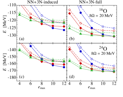
Figure 1: (color online) CCSD (dashed lines) and $\Lambda$CCSD(T) (solid lines) ground-state energies for ${}^{16}\text{O}$ and ${}^{24}\text{O}$ as function of $e_{\max}$ for the two types of Hamiltonians (see column headings) with $E_{3\max}=12$ for SRG flow parameters $\alpha$ set at $0.02\,\text{fm}^{4}$ ($\bullet$), $0.04\,\text{fm}^{4}$ (

$\blacksquare$

), and $0.08\,\text{fm}^{4}$ ($\blacktriangle$).

To assess the overall importance of triply excited clusters in nuclear-structure calculations, in Fig. 1 we compare the CCSD and $\Lambda$CCSD(T) ground-state energies $E^{\rm(CCSD)}$ and $E^{\rm({\Lambda}CCSD(T))}$ using the complete 3$N$ information, as function of $e_{\text{max}}$ for ${}^{16}\text{O}$ and ${}^{24}\text{O}$ and for the two 3$N$ Hamiltonians discussed in the previous section. First, we notice that we are reasonably converged within the model spaces we operate in and we observe the expected faster convergence with respect to model space-size for the softer, further evolved, interactions. Furthermore, the triples correction $\delta E^{\rm(T)}$ provides about 2–5 % of the binding energy for all nuclei considered, where, as expected, the contribution of the triply excited clusters decreases with the SRG flow parameter. Therefore, if one eventually aims at an accuracy in ground-state calculations of about 1 %, the truncation in the cluster operator $T$ is identified as one of the larger sources of error. The CCSD level of theory is not sufficiently accurate, the connected triply excited effects are not negligible, even for the softest interaction considered.

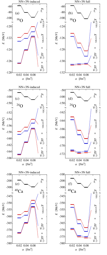
Figure 2: (color online) Anatomy of individual contributions from CCSD and $\Lambda$CCSD(T) to the total binding energy of ${}^{16,24}\text{O}$ and ${}^{40}\text{Ca}$ for the two types of Hamiltonians with $E_{3\max}=12$ and SRG flow parameters $\rm\alpha=0.02,0.04\ and\ 0.08\,\text{fm}^{4}$. For ${}^{16,24}\text{O}$, an $e_{\text{max}}=12$ model space and oscillator frequency $\hbar\Omega=20$ MeV was used, whereas for ${}^{40}\text{Ca}$ we work in an $e_{\text{max}}=10$ model space with $\hbar\Omega=24$ MeV.

Next we address the importance of the residual 3$N$ interaction in CCSD and $\Lambda$CCSD(T) calculations. Our discussion is complicated by the fact that energy values are not only determined by their expressions in terms of the $T^{\rm(CCSD)}$ and $\Lambda^{\rm(CCSD)}$ amplitudes $t^{a}_{i}$, $t^{ab}_{ij}$ and $\lambda^{i}_{a}$, $\lambda^{ij}_{ab}$, but also by the type of equations – with or without inclusion of the $W_{N}$ terms – used to determine the amplitudes. This leads to various possible and reasonable combinations to consider.

In Fig. 2, we show results for a series of increasingly complete calculations of the energy for ${}^{16}\text{O}$, ${}^{24}\text{O}$, and ${}^{40}\text{Ca}$ and for both the $NN+3N$-induced and $NN+3N$-full Hamiltonians. The energy $E_{\rm 2B}^{\rm(CCSD)}$ is calculated in NO2B approximation, i.e., the $W_{N}$ terms are neglected in the equations determining the $T^{\rm(CCSD)}$ amplitudes. For the calculation of all other energies we use $T^{\rm(CCSD)}$ and $\Lambda^{\rm(CCSD)}$ amplitudes determined from their respective amplitude equations including the $W_{N}$ terms. By comparing $E_{\rm 2B}^{\rm(CCSD)}$ with $E^{\rm(CCSD)}$, we obtain a direct quantification of the combined effect of the additional $W_{N}$ terms in the CCSD amplitude equations and energy expression. Note that $E^{\rm(CCSD)}-E_{\rm 2B}^{\rm(CCSD)}\neq\Delta E_{\rm 3B}^{\rm(CCSD)}$ here, due to the use of different amplitudes. The interesting question of whether the $W_{N}$ terms are more important in the determination of the amplitudes or in the energy expression will be adressed further below. Contrary to the previous situation, the same amplitudes are used in the calculation of $\delta E_{\rm 2B}^{\rm(T)}$ and $\delta E_{\rm 3B}^{\rm(T)}$. Therefore, using these numbers we can only quantify how important the $W_{N}$ contributions, given simply by $\delta E_{\rm 3B}^{\rm(T)}$, are in the calculation of the total triples correction $\delta E^{\rm(T)}$, i.e., we can compare the approximate energy expression $\tilde{E}^{\rm({\Lambda}CCSD(T))}$, Eq. (136), with the full form $E^{\rm({\Lambda}CCSD(T))}$, Eq. (131), but we cannot at the same time assess the relevance of $W_{N}$ terms in the respective equations determining the $T^{\rm(CCSD)}$ and $\Lambda^{\rm(CCSD)}$ amplitudes. Particularly for $\delta E_{\rm 2B}^{\rm(T)}$, other choices of where to include $W_{N}$ terms in the amplitude equations seem reasonable. We come back to this issue below but already mention here that for $\delta E_{\rm 2B}^{\rm(T)}$ other choices of amplitude equations lead to practically the same results.

All data shown in Fig. 2 are compiled in Table 3, and in the following we consider ${}^{16}\text{O}$ with the $NN$+3$N$-full Hamiltonian [Fig. 2(b)] at flow parameter values $\alpha$ = 0.02 ${\rm fm}^{4}\$and 0.08 ${\rm fm}^{4}\$as an example. When $\alpha$ increases, more and more of the binding energy is shifted to lower orders of the cluster expansion and the contributions from the higher orders consequently get smaller with the SRG flow: the magnitude of the reference energy $E_{\text{ref}}$ grows from –56.11 MeV to –101.67 MeV, while the CCSD correlation energy $\Delta E^{\rm(CCSD)}$ decreases from –69.03 MeV to –26.52 MeV as we go from $\alpha$ = 0.02 ${\rm fm}^{4}\$to 0.08 ${\rm fm}^{4}\$and the $\Lambda$CCSD(T) energy correction $\delta E^{\rm(T)}$, which we also consider as a measure for the contributions of the omitted cluster operators beyond the three-body level Binder et al. (2013), decreases from –5.54 MeV to –2.34 MeV, corresponding to 4.2 % and 1.8 % of the total binding energy. In the medium-mass regime considered here, these uncertainties related to the cluster truncation are typically the largest in our calculations for a given Hamiltonian, and therefore they determine the overall level of accuracy we aim at Binder et al. (2013).

Examining the contributions from the residual 3$N$ interaction to $\Delta E^{\rm(CCSD)}$ we find that, while the absolute value of $\Delta E^{\rm(CCSD)}$ decreases by about 30 MeV when we evolve the Hamiltonian from $\alpha$ = 0.02 ${\rm fm}^{4}\$further to 0.08 ${\rm fm}^{4}$, $\Delta E^{\rm(CCSD)}-\Delta E_{\rm 2B}^{\rm(CCSD)}$ is only subject to a slight increase from 0.54 MeV to 0.92 MeV, corresponding to 0.4 % and 0.7 % of the total binding energy. Consequently, the relative as well as the absolute importance of the residual 3$N$ interaction to the CCSD correlation energy grows with the SRG flow.

Furthermore, while for the harder Hamiltonian at $\alpha$ = 0.02 ${\rm fm}^{4}\$the $W_{N}$ contributions to $\Delta E^{\rm(CCSD)}$ are about one order of magnitude smaller than the accuracy level set by $\delta E^{\rm(T)}$, for the softer $\alpha$ = 0.08 ${\rm fm}^{4}\$Hamiltonian the $W_{N}$ contributions have an comparable size of about 39 % of the triples correction. Therefore, in order to keep different errors at a consistent level, for soft interactions the residual 3$N$ contributions should be included in CCSD if the triples correction is considered as well.

For the $\Lambda$CCSD(T) triples correction $\delta E^{\rm(T)}$ itself, the $W_{N}$ contributions $\delta E_{\rm 3B}^{\rm(T)}$, despite containing second-order MBPT contributions, have very small values of about –15 keV. This effect is about one order of magnitude smaller than the targeted accuracy given by the size of $\delta E^{\rm(T)}$ and may, therefore, be neglected. From another perspective, the $W_{N}$ contributions to $\delta E^{\rm(T)}$ constitute about 0.1 % of the total binding energy, which clearly is beyond the level of accuracy of any many-body method operating in the medium-mass regime today.

As is apparent from Fig. 2, the situation for the $NN+3N$-induced Hamiltonian and the heavier nuclei ${}^{24}\text{O}$ and ${}^{40}\text{Ca}$ is similar. In the case of ${}^{40}\text{Ca}$ we work in the smaller $e_{\text{max}}=10$ model space in order to keep the computational cost reasonable. In this model space the results are not fully converged with respect to $e_{\text{max}}$, but since the quality of the NO2B approximation is largely independent of $e_{\text{max}}$ Binder et al. (2013) this does not affect the present discussion. For the $NN+3N$-induced Hamiltonian, for example, the relative contribution of $W_{N}$ to the CCSD correlation energy grows from 1.3 % for $\alpha$ = 0.02 ${\rm fm}^{4}\$to 4.2 % for $\alpha$ = 0.08 ${\rm fm}^{4}$, in both cases constituting about 0.6 % of the total binding energy. Again, as the SRG flow parameter increases, the contributions of $W_{N}$ to the CCSD correlation energy on the one hand, and the triples correction on the other hand, become comparable; $\Delta E^{\rm(CCSD)}-\Delta E_{\rm 2B}^{\rm(CCSD)}$ is about 18 % of the size of the triples correction at $\alpha$ = 0.02 ${\rm fm}^{4}\$and already about 48 % at $\alpha$ = 0.08 ${\rm fm}^{4}$. The $W_{N}$ effect on the triples correction is again negligible, about one order of magnitude smaller than the triples correction itself, namely, about 2 % of $\delta E^{\rm(T)}$ for $\alpha$ = 0.02 ${\rm fm}^{4}\$and about 11 % for $\alpha$ = 0.08 ${\rm fm}^{4}$, or 0.1 % and 0.2 % of the total binding energy $E^{\rm({\Lambda}CCSD(T))}$.

It should be noted that the apparent flow-parameter independence of $E^{\rm({\Lambda}CCSD(T))}$ for the $NN+3N$-full Hamiltonian is accidental due to the $E_{3\max}$ cut used in our calculations. Increasing $E_{3\max}$ will move the energies upwards, and for the harder interactions it will do so to a larger extent than for the softer interactions. This leads to a reduction of the flow-parameter dependence of the $NN+3N$-induced results while the flow-parameter dependence of the $NN+3N$-full results is enhanced Binder et al. (2013)..

In summary, for hard interactions, the residual 3$N$ effects to the CCSD correlation energy $E^{\rm(CCSD)}$ are rather small compared to the triples correction $\delta E^{\rm(T)}$, but they become comparable for soft interactions. Therefore, when using soft interactions, the residual 3$N$ interaction should be included in CCSD if the desired accuracy level also demands inclusion of triples excitation effects. For the triples correction, on the other hand, the residual 3$N$ interaction only plays an insignificant role, providing contributions that are shadowed by the considerably larger uncertainties stemming, e.g., from the cluster truncation. This motivates the use of the truncated energy expression $\tilde{E}^{\rm({\Lambda}CCSD(T))}$, Eq. (136), instead of the full form $E^{\rm({\Lambda}CCSD(T))}$, Eq. (131), resulting in only negligible losses in accuracy.

Table 3: Summary of the individual contributions to the $\Lambda$CCSD(T) ground-state energies in MeV for ${}^{16}\text{O}$, ${}^{24}\text{O}$, and ${}^{40}\text{Ca}$ and for the $NN+3N$-induced and $NN+3N$-full Hamiltonians with $E_{3\max}=12$, obtained for ${}^{16}\text{O}$ and ${}^{24}\text{O}$ from an $e_{\text{max}}=12$ model space with oscillator frequency $\hbar\Omega=20$ MeV and for ${}^{40}\text{Ca}$ from an $e_{\text{max}}=10$ model space with $\hbar\Omega=24$ MeV. For the calculation of $\Delta E_{\rm 2B}^{\rm(CCSD)}$, amplitudes from the NO2B approximation have been used, while for the calculation of all other quantities the required amplitudes have been determined from equations including the residual 3$N$ interaction.

NN+3N-	$\alpha\,[\text{fm}^{4}]$	$E^{\rm({\Lambda}CCSD(T))}$	$E_{\text{ref}}$	$\Delta E_{\rm 2B}^{\rm(CCSD)}$	$\Delta E^{\rm(CCSD)}-\Delta E_{\rm 2B}^{\rm(CCSD)}$	$\delta E_{\rm 2B}^{\rm(T)}$	$\delta E_{\rm 3B}^{\rm(T)}$
induced
${}^{16}\text{O}$	0.02	–126.37	–56.47	–66.05	0.67	–4.46	–0.06
	0.04	–124.09	–80.09	–41.93	0.86	–2.83	–0.10
	0.08	–121.78	–96.59	–24.28	0.90	–1.66	–0.15
${}^{24}\text{O}$	0.02	–164.92	–65.41	–93.22	0.89	–7.01	–0.18
	0.04	–161.14	–98.32	–59.23	1.15	–4.56	–0.18
	0.08	–156.97	–120.64	–34.52	1.19	–2.75	–0.24
${}^{40}\text{Ca}$	0.02	–372.25	–186.58	–174.35	2.44	–13.44	–0.31
	0.04	–364.87	–252.67	–106.28	2.78	–8.22	–0.49
	0.08	–353.00	–291.98	–58.32	2.46	–4.56	–0.59
NN+3N-	$\alpha[\text{fm}^{4}]$	$E^{\rm({\Lambda}CCSD(T))}$	$E_{\text{ref}}$	$\Delta E_{\rm 2B}^{\rm(CCSD)}$	$\Delta E^{\rm(CCSD)}-\Delta E_{\rm 2B}^{\rm(CCSD)}$	$\delta E_{\rm 2B}^{\rm(T)}$	$\delta E_{\rm 3B}^{\rm(T)}$
full
${}^{16}\text{O}$	0.02	–130.68	–56.11	–69.57	0.54	–5.39	–0.15
	0.04	–130.61	–81.79	–45.87	0.82	–3.61	–0.16
	0.08	–130.51	–101.67	–27.44	0.92	–2.17	–0.17
${}^{24}\text{O}$	0.02	–171.28	–64.16	–99.53	0.67	–8.01	–0.25
	0.04	–171.82	–101.52	–65.81	1.07	–5.28	–0.28
	0.08	–171.65	–130.43	–39.01	1.18	–3.05	–0.35
${}^{40}\text{Ca}$	0.02	–369.56	–158.28	–194.80	2.12	–17.80	–0.80
	0.04	–375.02	–238.62	–126.64	2.96	–11.86	–0.86
	0.08	–375.82	–298.75	–72.23	2.85	–6.82	–0.87

The above considerations indicate that the residual 3$N$ interaction may be neglected in calculating the $\Lambda$CCSD(T) energy correction $\delta E^{\rm(T)}$ without significantly affecting the overall accuracy, leading to Eq. (136) as an approximate form for $E^{\rm({\Lambda}CCSD(T))}$. From a practitioner’s point of view, discarding the $W_{N}$ contributions to $\delta E^{\rm(T)}$, Eqs. (128)–(129), already leads to significant savings in the implementational effort and computing time which in our calculations requires about half a million CPU hours for one $\delta E^{\rm(T)}$ evaluation for ${}^{16}\text{O}$ calculation at $e_{\text{max}}=12$ using full $W_{N}$ information with $E_{3\max}=12$, which is about two orders of magnitude more computationally expensive than the analogous calculation using the NO2B approximation. However, one still has to solve the CCSD equations determining the $T^{\rm(CCSD)}$ amplitudes $t^{a}_{i}$ and $t^{ab}_{ij}$ as well as the $\Lambda$CCSD equations determining the $\Lambda^{\rm(CCSD)}$ amplitudes $\lambda^{i}_{a}$ and $\lambda^{ij}_{ab}$ with full incorporation of $W_{N}$. Particularly solving the $\Lambda$CCSD equations, for which the similarity-transformed Hamiltonian contributions given in Tables 1 and 2 have to be evaluated, consumes lots of the computing time in our calculations. Therefore, it is also worthwhile to investigate how much of the residual 3$N$ information has to be incluced in solving for the amplitudes of the $T^{\rm(CCSD)}$ and $\Lambda^{\rm(CCSD)}$ operators that enter the energy expressions, in order to obtain accurate results at the lowest possible computational cost.

In order to distinguish different approximation schemes, we introduce the notation in which for energy quantities that only depend on $T^{\rm(CCSD)}$ amplitudes the label in brackets denotes if the $T^{\rm(CCSD)}$ amplitudes were determined from the amplitude equations with (3B) or without residual 3$N$ interaction (2B). Similarly, for quantities that depend on both $T^{\rm(CCSD)}$ and $\Lambda^{\rm(CCSD)}$ amplitudes, the first label denotes the type of equation used to determine the $T^{\rm(CCSD)}$ amplitudes and the second one identifies the $\Lambda$CCSD equations. For example, $\tilde{E}^{\rm({\Lambda}CCSD(T))}{\rm(3B,2B)}$ refers to the energy expression (136), calculated using $T^{\rm(CCSD)}$ amplitudes determined from Eqs. (58), (59), (60) and (61) and the $\Lambda^{\rm(CCSD)}$ amplitudes determined from Eqs. (79) and (80) only.

We consider the following approximation schemes, in which the $W_{N}$ contributions $\delta E_{\rm 3B}^{\rm(T)}$ to the triples correction are always neglected: For the “NO2B” scheme, all $W_{N}$ terms are discarded in both the determination of the $T^{\rm(CCSD)}$ and $\Lambda^{\rm(CCSD)}$ amplitudes and the calculation of the energy $E_{\rm 2B}^{\rm({\Lambda}CCSD(T))}$, Eq. (132),

$$E^{\rm(NO2B)}=E_{\rm 2B}^{\rm({\Lambda}CCSD(T))}{\rm(2B,2B)}\ .$$ (137)

This of course corresponds to an ordinary $\Lambda$CCSD(T) calculation in NO2B approximation. For scheme “A”, we compute $E_{\rm 2B}^{\rm({\Lambda}CCSD(T))}$ as in the NO2B case and also add $\Delta E_{\rm 3B}^{\rm(CCSD)}$ with $T^{\rm(CCSD)}$ amplitudes obtained from the NO2B CCSD calculation,

$$E^{\rm(A)}=E_{\rm 2B}^{\rm({\Lambda}CCSD(T))}{\rm(2B,2B)}+\Delta E_{\rm 3B}^{\rm(CCSD)}{\rm(2B)}\ .$$ (138)

This represents the simplest and most economic way to include $W_{N}$ information, where it only enters in the expression for the energy contribution $\Delta E_{\rm 3B}^{\rm(CCSD)}$, Eq. (66), but not in the considerably more complex equations that determine the amplitudes. In scheme “B”, we include full $W_{N}$ information in the calculation of the CCSD correlation energy, keeping the $W_{N}$ terms in the amplitude equations as well as in the energy expression. The triples correction, however, is calculated without any $W_{N}$ information,

$$E^{\rm(B)}=E^{\rm(CCSD)}{\rm(3B)}+\delta E_{\rm 2B}^{\rm(T)}{\rm(2B,2B)}\ .$$ (139)

This way we keep consistency between the $T^{\rm(CCSD)}$ and $\Lambda^{\rm(CCSD)}$ amplitudes that enter the triples correction, while capturing all residual 3$N$ effects in the CCSD energy $\Delta E^{\rm(CCSD)}$. In scheme “C”, we introduce an inconsistency between the $T^{\rm(CCSD)}$ and $\Lambda^{\rm(CCSD)}$ amplitudes by solving for $T^{\rm(CCSD)}$ with the $W_{N}$ terms present, while neglecting the $W_{N}$ terms in the equations for $\Lambda^{\rm(CCSD)}$, and calculate the energy using Eq. (136),

$$E^{\rm(C)}=\tilde{E}^{\rm({\Lambda}CCSD(T))}{\rm(3B,2B)}\ .$$ (140)

This variant is reasonable since one typically has to solve for the $T^{\rm(CCSD)}$ amplitude equations with $W_{N}$ terms anyway in order to obtain the comparatively large $\Delta E_{\rm 3B}^{\rm(CCSD)}$ contribution to the energy while one would like to avoid to solve for the $\Lambda^{\rm(CCSD)}$ amplitudes in this manner, if the resulting energies do not change much. Finally, in scheme “D”, in which we only neglect the residual 3$N$ interaction terms in the expression for $\delta E^{\rm(T)}$, we use the full, $W_{N}$-containing equations to solve for the $T^{\rm(CCSD)}$ and $\Lambda^{\rm(CCSD)}$ amplitudes and determine the energy via Eq. (136),

$$E^{\rm(D)}=\tilde{E}^{\rm({\Lambda}CCSD(T))}{\rm(3B,3B)}\ .$$ (141)

As in the discussion of Fig. 2, this variant allows to estimate the importance of $W_{N}$ for the $\Lambda^{\rm(CCSD)}$ amplitudes.

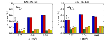
Figure 3: (color online) Comparison of the deviations introduced by the different approximation schemes, Eqs. (137)–(141), described in the text from the full inclusion of the residual $3N$ interaction in all steps involving a CCSD and $\Lambda$CCSD(T) calculation.

In Fig. 3, for the case of ${}^{16}\text{O}$, ${}^{40}\text{Ca}$ and the $NN+3N$-full Hamiltonian, we compare the deviations of all the aforementioned approximation schemes from the complete 3$N$ calculations. For ${}^{24}\text{O}$ and the $NN+3N$-induced Hamiltonian we obtain very similar results. As expected, the “NO2B” scheme shows the largest deviations because the contributions of $W_{N}$ to CCSD are completely missing. Including the $W_{N}$ terms in the energy expression for the CCSD correlation energy but evaluating it using $T^{\rm(CCSD)}$ amplitudes without $W_{N}$ information in scheme “A” virtually does not change the “NO2B” results. Therefore, we can conclude that it is the $W_{N}$ effect on the $T^{\rm(CCSD)}$ amplitudes that is most important for CCSD, and not the additional terms in $\Delta E_{\rm 3B}^{\rm(CCSD)}$. In our calculations, the best approximation to the complete inclusion of residual 3$N$ interactions is provided by scheme “B”, where we use full $W_{N}$ information to determine the CCSD correlation energy, but otherwise no $W_{N}$ information enters the calculation of the triples correction. However, approximation schemes “B”,“C”, and “D” give very similar results, again hinting at the $W_{N}$ effect on the $T^{\rm(CCSD)}$ amplitudes to be the most important ingredient in the inclusion of residual 3$N$ interactions in CCSD and $\Lambda$CCSD(T) calculations.

IV Conclusions

In this article we considered the extension of CC theory with a full treatment of singly and doubly excited clusters and a non-iterative treatment of triply excited clusters to three-body Hamiltonians. The incorporation of 3$N$ interactions into CCSD was previously discussed in detail in Ref. Hagen et al. (2007), so in this article we focused on the corresponding generalization of the non-iterative treatment of triply excited clusters. Among various triples corrections, for this first study we chose the $\Lambda$CCSD(T)-type approach due to its relatively simple structure.

The $\Lambda$CCSD(T) approach requires one to solve the $\Lambda$CCSD equations prior to the computation of the actual energy correction. Thus, in addition to the explicit energy expressions defining the $\Lambda$CCSD(T) approach for three-body Hamiltonians, we also provided a detailed discussion of the inclusion of 3$N$ interactions into the $\Lambda$CCSD equations, listing the complete set of the relevant programmable expressions. The similarity-transformed Hamiltonian is a central quantity of coupled-cluster theory and in this article we give explicit expressions for the contributions of the residual 3$N$ interactions to all one- and two-body components as well as selected three- and four-body components of this Hamiltonian. We derived the $\Lambda$CCSD(T) method as an approximation to the more complete CR-CC(2,3) approach which allows for an easy identification of new terms arising due to the presence of residual 3$N$ interactions, and we provided complete and explicit expressions required in the calculation of the $\Lambda$CCSD(T) energy correction for three-body Hamiltonians.

One of the important outcomes of our analysis is the realization that through the use of explicit 3$N$ interactions in $\Lambda$CCSD(T), compared to the approximate NO2B treatment, contributions of the triply excited clusters are moved from second to first order in MBPT for the wave function, and from fourth to second order for the energy. This is rather easy to account for at the full CCSDT level, which is, unfortunately prohibitively expensive, but is not trivial at all when one tries to account for the $T_{3}$ cluster contributions via corrections to the CCSD energy. The use of the CR-CC(2,3) formalism, which contains the $\Lambda$CCSD(T) approach as an approximation, turned out to be central for properly accounting for the second-order MBPT corrections due to the $T_{3}$ clusters induced by residual 3$N$ interactions and other related terms.

The method was applied to the medium-mass closed-shell nuclei ${}^{16}\text{O}$, ${}^{24}\text{O}$ and ${}^{40}\text{Ca}$ using $NN+3N$ Hamiltonians obtained from chiral EFT. For the total binding energies, the effect of the residual three-body interactions at the level of CCSD can become comparable to the $\Lambda$CCSD(T) correction, particularly for soft interactions, while for the $\Lambda$CCSD(T) correction itself, contributions of the residual 3$N$ interactions were shown to be negligible. Therefore, for the CCSD and $\Lambda$CCSD(T) calculations, by only including explicit 3$N$ interactions at the CCSD level, we can practically eliminate the error introduced by the normal-ordering approximation. We further discussed various combinations of where to include the residual 3$N$ interactions in the determination of the amplitudes from which energies are calculated, and found that the residual 3$N$ interactions have their most significant effect on the cluster amplitudes, i.e., it is important to solve the CCSD equations including residual 3$N$ interactions when determining the CCSD energy, but one can safely neglect these interactions in post-CCSD corrections due to $T_{3}$ clusters.

V Acknowledgments

Numerical calculations have been performed at the Jülich Supercomputing Centre, at the LOEWE-CSC Frankfurt, and at the National Energy Research Scientific Computing Center supported by the Office of Science of the U.S. Department of Energy under Contract No. DE-AC02-05CH11231. Supported by the Deutsche Forschungsgemeinschaft through contract SFB 634, by the Helmholtz International Center for FAIR within the LOEWE program of the State of Hesse, and the BMBF through contracts 06DA9040I and 06DA7047I. Additional support by the Chemical Sciences, Geosciences and Biosciences Division, Office of Basic Energy Sciences, Office of Science, U.S. Department of Energy (Grant No. DE-FG02-01ER15228 to P.P.) is gratefully acknowledged. P.N. acknowledges support from Natural Sciences and Engineering Research Council of Canada (NSERC) Grant No. 401945-2011.

References

- Weinberg (1979) S. Weinberg, Physica A 96, 327 (1979).
- Gasser and Leutwyler (1984) J. Gasser and H. Leutwyler, Ann. Phys. 158, 142 (1984).
- Weinberg (1990) S. Weinberg, Phys. Lett. B 251, 288 (1990).
- Weinberg (1991) S. Weinberg, Nucl. Phys. B 363, 3 (1991).
- van Kolck (1999) U. van Kolck, Prog. Part. Nucl. Phys. 43, 337 (1999).
- Epelbaum et al. (2009) E. Epelbaum, H.-W. Hammer, and U.-G. Meißner, Rev. Mod. Phys. 81, 1773 (2009).
- Machleidt and Entem (2011) R. Machleidt and D. R. Entem, Phys. Rep. 503, 1 (2011).
- Navrátil et al. (2007) P. Navrátil, V. G. Gueorguiev, J. P. Vary, W. E. Ormand, and A. Nogga, Phys. Rev. Lett. 99, 042501 (2007).
- Nogga et al. (2006) A. Nogga, P. Navrátil, B. R. Barrett, and Vary J. P., Phys. Rev. C 73, 064002 (2006).
- Roth et al. (2011) R. Roth, J. Langhammer, A. Calci, S. Binder, and P. Navrátil, Phys. Rev. Lett. 107, 072501 (2011).
- Roth et al. (2012) R. Roth, S. Binder, K. Vobig, A. Calci, J. Langhammer, and P. Navrátil, Phys. Rev. Lett. 109, 052501 (2012).
- Maris et al. (2013) P. Maris, J. P. Vary, and P. Navrátil, Phys. Rev. C 87, 014327 (2013).
- Hergert et al. (2013a) H. Hergert, S. K. Bogner, S. Binder, A. Calci, J. Langhammer, R. Roth, and A. Schwenk, Phys. Rev. C 87, 034307 (2013a).
- Hergert et al. (2013b) H. Hergert, S. Binder, A. Calci, J. Langhammer, and R. Roth, Phys. Rev. Lett. 110, 242501 (2013b).
- Navrátil et al. (2000a) P. Navrátil, J. P. Vary, and B. R. Barrett, Phys. Rev. Lett. 84, 5728 (2000a).
- Navrátil et al. (2000b) P. Navrátil, G. P. Kamuntavicius, and B. R. Barrett, Phys. Rev. C 61, 044001 (2000b).
- Navrátil and Ormand (2002) P. Navrátil and W. E. Ormand, Phys. Rev. Lett. 88, 152502 (2002).
- Roth and Navrátil (2007) R. Roth and P. Navrátil, Phys. Rev. Lett. 99, 092501 (2007).
- Caurier et al. (2005) E. Caurier, G. Martínez-Pinedo, F. Nowacki, A. Poves, and A. Zuker, Rev. Mod. Phys. 55, 427 (2005).
- Navrátil et al. (2009) P. Navrátil, S. Quaglioni, I. Stetcu, and B. Barrett, J. Phys. G: Nucl. Part. Phys. 36, 083101 (2009).
- Roth (2009) R. Roth, Phys. Rev. C 79, 064324 (2009).
- Roth et al. (2009a) R. Roth, J. R. Gour, and P. Piecuch, Phys. Rev. C 79, 054325 (2009a).
- Coester (1958) F. Coester, Nucl. Phys. 7, 421 (1958).
- Coester and Kümmel (1960) F. Coester and H. Kümmel, Nucl. Phys. 17, 477 (1960).
- Kümmel et al. (1978) H. Kümmel, K. H. Lührmann, and J. G. Zabolitzky, Phys. Rep. 36, 1 (1978).
- Čížek (1966) J. Čížek, J. Chem. Phys. 45, 4256 (1966).
- Čížek (1969) J. Čížek, Adv. Chem. Phys. 14, 35 (1969).
- Čížek and Paldus (1971) J. Čížek and J. Paldus, Int. J. Quantum Chem. 5, 359 (1971).
- Paldus et al. (1972) J. Paldus, I. Shavitt, and J. Čížek, Phys. Rev. A 5, 50 (1972).
- Bishop (1998) R. F. Bishop, in Microscopic Quantum Many-Body Theories and Their Applications, edited by J. Navarro and A. Polls (Springer, Berlin, 1998), vol. 510 of Lecture Notes in Physics, pp. 119–206.
- Purvis and Bartlett (1982) G. D. Purvis, III and R. J. Bartlett, J. Chem. Phys. 76, 1910 (1982).
- Cullen and Zerner (1982) J. M. Cullen and M. C. Zerner, J. Chem. Phys. 77, 4088 (1982).
- Kowalski et al. (2004) K. Kowalski, D. J. Dean, M. Hjorth-Jensen, T. Papenbrock, and P. Piecuch, Phys. Rev. Lett. 92, 132501 (2004).
- Dean and Hjorth-Jensen (2004) D. J. Dean and M. Hjorth-Jensen, Phys. Rev. C 69, 054320 (2004).
- Włoch et al. (2005a) M. Włoch, D. J. Dean, J. R. Gour, P. Piecuch, M. Hjorth-Jensen, T. Papenbrock, and K. Kowalski, Eur. Phys. J. A 25, 485 (2005a).
- Włoch et al. (2005b) M. Włoch, J. R. Gour, P. Piecuch, D. J. Dean, M. Hjorth-Jensen, and T. Papenbrock, J. Phys. G: Nucl. Part. Phys. 31, S1291 (2005b).
- Włoch et al. (2005c) M. Włoch, D. J. Dean, J. R. Gour, M. Hjorth-Jensen, K. Kowalski, T. Papenbrock, and P. Piecuch, Phys. Rev. Lett. 94, 212501 (2005c).
- Horoi et al. (2007) M. Horoi, J. R. Gour, M. Włoch, M. D. Lodriguito, B. A. Brown, and P. Piecuch, Phys. Rev. Lett. 98, 112501 (2007).
- Hagen et al. (2008) G. Hagen, T. Papenbrock, D. J. Dean, and M. Hjorth-Jensen, Phys. Rev. Lett. 101, 092502 (2008).
- Hagen et al. (2009a) G. Hagen, T. Papenbrock, D. J. Dean, M. Hjorth-Jensen, and B. V. Asokan, Phys. Rev. C 80, 021306 (2009a).
- Roth et al. (2009b) R. Roth, J. R. Gour, and P. Piecuch, Phys. Lett. B 679, 334 (2009b).
- Hagen et al. (2012) G. Hagen, M. Hjorth-Jensen, G. R. Jansen, R. Machleidt, and T. Papenbrock, Phys. Rev. Lett. 109, 032502 (2012).
- Hagen et al. (2007) G. Hagen, T. Papenbrock, D. J. Dean, A. Schwenk, A. Nogga, M. Włoch, and P. Piecuch, Phys. Rev. C 76, 034302 (2007).
- Binder et al. (2013) S. Binder, J. Langhammer, A. Calci, P. Navrátil, and R. Roth, Phys. Rev. C 87, 021303(R) (2013).
- Raghavachari et al. (1989) K. Raghavachari, G. W. Trucks, J. A. Pople, and M. Head-Gordon, Chem. Phys. Lett. 102, 479 (1989).
- Dean et al. (2005) D. J. Dean, J. R. Gour, G. Hagen, M. Hjorth-Jensen, K. Kowalski, T. Papenbrock, P. Piecuch, and M. Włoch, Nucl. Phys. A 752, 299 (2005).
- Piecuch and Kowalski (2000) P. Piecuch and K. Kowalski, in Computational Chemistry: Reviews of Current Trends, edited by J. Leszczyński (World Scientific, Singapore, 2000), vol. 5, pp. 1–104.
- Kowalski and Piecuch (2000a) K. Kowalski and P. Piecuch, J. Chem. Phys. 113, 18 (2000a).
- Kowalski and Piecuch (2000b) K. Kowalski and P. Piecuch, J. Chem. Phys. 113, 5644 (2000b).
- Piecuch et al. (2002) P. Piecuch, K. Kowalski, I. S. O. Pimienta, and M. J. McGuire, Int. Rev. Phys. Chem. 21, 527 (2002).
- Piecuch et al. (2004) P. Piecuch, K. Kowalski, I. S. O. Pimienta, P.-D. Fan, M. Lodriguito, M. J. McGuire, S. A. Kucharski, T. Kuś, and M. Musiał, Theor. Chem. Acc. 112, 349 (2004).
- Gwaltney and Head-Gordon (2000) S. R. Gwaltney and M. Head-Gordon, Chem. Phys. Lett. 323, 21 (2000).
- Gwaltney and Head-Gordon (2001) S. R. Gwaltney and M. Head-Gordon, J. Chem. Phys. 115, 2014 (2001).
- Hirata et al. (2001) S. Hirata, M. Nooijen, I. Grabowski, and R. J. Bartlett, J. Chem. Phys. 114, 3919 (2001), 115, 3967 (2001) [Erratum].
- Hirata et al. (2004) S. Hirata, P.-D. Fan, A. A. Auer, M. Nooijen, and P. Piecuch, J. Chem. Phys. 121, 12197 (2004).
- Kucharski and Bartlett (1998) S. A. Kucharski and R. J. Bartlett, J. Chem. Phys. 108, 5243 (1998).
- Taube and Bartlett (2008a) A. G. Taube and R. J. Bartlett, J. Chem. Phys. 128, 044110 (2008a).
- Taube and Bartlett (2008b) A. G. Taube and R. J. Bartlett, J. Chem. Phys. 128, 044111 (2008b).
- Hagen et al. (2010) G. Hagen, T. Papenbrock, D. J. Dean, and M. Hjorth-Jensen, Phys. Rev. C 82, 034330 (2010).
- Piecuch and Włoch (2005) P. Piecuch and M. Włoch, J. Chem. Phys. 123, 224105 (2005).
- Piecuch et al. (2006a) P. Piecuch, M. Włoch, J. R. Gour, and A. Kinal, Chem. Phys. Lett. 418, 467 (2006a).
- Włoch et al. (2007) M. Włoch, J. R. Gour, and P. Piecuch, J. Phys. Chem. A 111, 11359 (2007).
- Piecuch et al. (2009) P. Piecuch, J. R. Gour, and M. Włoch, Int. J. Quantum Chem. 109, 3268 (2009).
- Tsukiyama et al. (2011) K. Tsukiyama, S. K. Bogner, and A. Schwenk, Phys. Rev. Lett. 106, 222502 (2011).
- Papenbrock et al. (2006) T. Papenbrock, D. J. Dean, J. R. Gour, G. Hagen, M. Hjorth-Jensen, P. Piecuch, and M. Włoch, Int. J. Mod. Phys. B 20, 5338 (2006).
- Heisenberg and Mihaila (1999) J. H. Heisenberg and B. Mihaila, Phys. Rev. C 59, 1440 (1999).
- Ge et al. (2007) Y. B. Ge, M. S. Gordon, and P. Piecuch, J. Chem. Phys. 127, 174106 (2007).
- Ge et al. (2008) Y. B. Ge, M. S. Gordon, P. Piecuch, M. Włoch, and J. R. Gour, J. Phys. Chem. A 112, 11873 (2008).
- Taube (2010) A. G. Taube, Mol. Phys. 108, 2951 (2010).
- Shen and Piecuch (2012) J. Shen and P. Piecuch, Chem. Phys. 401, 180 (2012).
- Noga and Bartlett (1987) J. Noga and R. J. Bartlett, J. Chem. Phys. 86, 7041 (1987), 89, 3401 (1988) [Erratum].
- Scuseria and Schaefer (1988) G. E. Scuseria and H. F. Schaefer, III, Chem. Phys. Lett. 152, 382 (1988).
- Gauss (1998) J. Gauss, in Encyclopedia of Computational Chemistry, edited by P. v. R. Schleyer, N. L. Allinger, T. Clark, J. Gasteiger, P. A. Kollman, H. F. Schaefer, III, and P. R. Schreiner (Wiley, Chichester, 1998), vol. 1, pp. 615–636.
- Paldus and Li (1999) J. Paldus and X. Li, Adv. Chem. Phys. 110, 1 (1999).
- Piecuch et al. (2006b) P. Piecuch, M. Włoch, M. Lodriguito, and J. R. Gour, in Recent Advances in the Theory of Chemical and Physical Systems, edited by S. Wilson, J.-P. Julien, J. Maruani, E. Brändas, and G. Delgado-Barrio (Springer, Dordrecht, 2006b), vol. 15 of Progress in Theoretical Chemistry and Physics, pp. 45–106.
- Bartlett and Musiał (2007) R. J. Bartlett and M. Musiał, Rev. Mod. Phys. 79, 291 (2007).
- Piecuch et al. (2005) P. Piecuch, M. Włoch, J. R. Gour, D. J. Dean, M. Hjorth-Jensen, and T. Papenbrock, in Nuclei and Mesoscopic Physics: Workshop on Nuclei and Mescopic Physics WNMP 2004, edited by V. Zelevinsky (American Institute of Physics, Melville, New York, 2005), vol. 777 of AIP Conference Proceedings, pp. 28–45.
- Salter et al. (1989) E. A. Salter, G. W. Trucks, and R. J. Bartlett, J. Chem. Phys. 90, 1752 (1989).
- Gauss et al. (1991) J. Gauss, J. F. Stanton, and R. J. Bartlett, J. Chem. Phys. 95, 2623 (1991).
- Stanton and Bartlett (1993) J. F. Stanton and R. J. Bartlett, J. Chem. Phys. 98, 7029 (1993).
- Piecuch and Bartlett (1999) P. Piecuch and R. J. Bartlett, Adv. Quantum Chem. 34, 295 (1999).
- Gour et al. (2006) J. R. Gour, P. Piecuch, M. Hjorth-Jensen, M. Włoch, and D. J. Dean, Phys. Rev. C 74, 024310 (2006).
- Scuseria et al. (1987) G. E. Scuseria, A. C. Scheiner, T. J. Lee, J. E. Rice, and H. F. Schaefer, III, J. Chem. Phys. 86, 2881 (1987).
- Piecuch and Paldus (1989) P. Piecuch and J. Paldus, Int. J. Quantum Chem. 36, 429 (1989).
- Włoch et al. (2005d) M. Włoch, J. R. Gour, K. Kowalski, and P. Piecuch, J. Chem. Phys. 122, 214107 (2005d).
- Urban et al. (1985) M. Urban, J. Noga, S. J. Cole, and R. J. Bartlett, J. Chem. Phys. 83, 4041 (1985).
- Piecuch and Paldus (1990) P. Piecuch and J. Paldus, Theor. Chim. Acta 78, 65 (1990).
- Kucharski and Bartlett (1998) S. Kucharski and R. Bartlett, J. Chem. Phys. 108, 9221 (1998).
- Musiał and Bartlett (2010) M. Musiał and R. J. Bartlett, J. Chem. Phys. 133, 104102 (2010).
- Piecuch et al. (2008) P. Piecuch, M. Włoch, and A. J. C. Varandas, Theor. Chem. Acc. 120, 59 (2008).
- Kowalski and Piecuch (2005) K. Kowalski and P. Piecuch, J. Chem. Phys. 122, 074107 (2005).
- Koch and Jørgensen (1990) H. Koch and P. Jørgensen, J. Chem. Phys. 93, 3333 (1990).
- Arponen (1983) J. S. Arponen, Ann. Phys. 151, 311 (1983).
- Arponen et al. (1987) J. S. Arponen, R. F. Bishop, and E. Pajanne, Phys. Rev. A 36, 2519 (1987).
- Szalay et al. (1995) P. G. Szalay, M. Nooijen, and R. J. Bartlett, J. Chem. Phys. 103, 281 (1995).
- Moszyński and Jeziorski (1993) R. Moszyński and B. Jeziorski, Int. J. Quantum Chem. 48, 161 (1993).
- Bartlett (1995) R. J. Bartlett, in Modern Electronic Structure Theory, Part I, edited by D. R. Yarkony (World Scientific, Singapore, 1995), pp. 1047–1131.
- Löwdin (1962) P.-O. Löwdin, J. Math. Phys. 3, 969 (1962).
- Stanton (1997) J. F. Stanton, Chem. Phys. Lett. 281, 130 (1997).
- Jankowski et al. (1991) K. Jankowski, J. Paldus, and P. Piecuch, Theor. Chim. Acta 80, 223 (1991).
- Entem and Machleidt (2003) D. R. Entem and R. Machleidt, Phys. Rev. C 68, 041001(R) (2003).
- Navrátil (2007) P. Navrátil, Few Body Syst. 41, 117 (2007).
- Jurgenson et al. (2009) E. D. Jurgenson, P. Navrátil, and R. J. Furnstahl, Phys. Rev. Lett. 103, 082501 (2009).
- Roth et al. (2010) R. Roth, T. Neff, and H. Feldmeier, Prog. Part. Nucl. Phys. 65, 50 (2010).
- (105) R. Roth, A. Calci, J. Langhammer, and S. Binder, in preparation.
- Hagen et al. (2009b) G. Hagen, T. Papenbrock, and D. Dean (2009b), arXiv:0905.3167v1 [nucl-th].