Stress concentration near stiff inclusions:
validation of rigid inclusion model and boundary layers
by means of photoelasticity

Abstract

Photoelasticity is employed to investigate the stress state near stiff rectangular and rhombohedral inclusions embedded in a ‘soft’ elastic plate. Results show that the singular stress field predicted by the linear elastic solution for the rigid inclusion model can be generated in reality, with great accuracy, within a material. In particular, experiments: (i.) agree with the fact that the singularity is lower for obtuse than for acute inclusion angles; (ii.) show that the singularity is stronger in Mode II than in Mode I (differently from a notch); (iii.) validate the model of rigid quadrilateral inclusion; (iv.) for thin inclusions, show the presence of boundary layers deeply influencing the stress field, so that the limit case of rigid line inclusion is obtained in strong dependence on the inclusion’s shape. The introduced experimental methodology opens the possibility of enhancing the design of thin reinforcements and of analyzing complex situations involving interaction between inclusions and defects.

Keywords: High-contrast composites; rigid wedge; stiff phases; singular elastic fields, stiffener.

1 Introduction

Experimental stress analysis near a crack or a void has been the subject of an intense research effort (see for instance Lim and Ravi-Chandar, 2007; 2009; Schubnel et al. 2011; Templeton et al. 2009), but the stress field near a rigid inclusion embedded in an elastic matrix, a fundamental problem in the design of composites, has surprisingly been left almost unexplored (Theocaris, 1975; Theocaris and Paipetis, 1976 a; b; Reedy and Guess, 2001) and has never been investigated via photoelasticity.

Though the analytical determination of elastic fields around inclusions is a problem in principle solvable with existing methodologies (Movchan and Movchan, 1995; Muskhelishvili, 1953; Savin, 1961), detailed treatments are not available and the existing solutions lack mechanical interpretation, in the sense that it is not known if these predict stress fields observable in reality. Moreover, from experimental point of view, questions arise whether the bonding between inclusion and matrix can be realized and can resist loading without detachment (which would introduce a crack) and if self-stresses can be reduced to negligible values. In this article we (i.) re-derive asymptotic and full-field solutions for rectangular and rhombohedral rigid inclusions (Section 2) and (ii.) compare these with photoelastic experiments (Section 3).

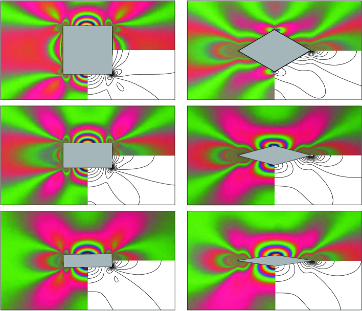
Figure 1: Photoelastic fringes revealing the stress field near stiff (made up of polycarbonate, Young modulus 2350 MPa) rectangular (large edge $l_{x}=$20 mm, edges aspect ratios $l_{y}/l_{x}=\{1;1/2;1/4\}$) and rhombohedral (large axis $l_{x}=$30 mm, axis aspect ratios $l_{y}/l_{x}=\{9/15;4/15;2/15\}$) inclusions embedded in an elastic matrix (a two-component epoxy resin, Young modulus 22 MPa, approximatively 100 times less stiff than the inclusions) and loaded with a remote uniaxial tensile stress $\sigma_{xx}^{\infty}=$0.28 MPa, compared to the elastic solution for rigid inclusions (in plane stress, with Poisson’s ratio equal to 0.49).

Photoelastic fringes obtained with a white circular polariscope are shown in Fig. 1 and indicate that the linear elastic solutions provide an excellent description of the elastic fields generated by inclusions up to a distance so close to the edges of the inclusions that fringes result unreadable (even with the aid of an optical microscope). By comparison of the photos shown in Fig. 1 with Fig. 1 of Noselli et al. (2010), it can be noted that the stress fields correctly tend to those relative to a rigid line inclusion (stiffener), when the aspect ratio of the inclusions decreases, and that the stress fields very close to a thin inhomogeneity are substantially affected by boundary layers depending on the (rectangular or rhombohedral) shape.

2 Theoretical linear elastic fields near rigid polygonal inclusions

The stress/strain fields in a linear isotropic elastic matrix containing a rigid polygonal inclusion are obtained analytically through both an asymptotic approach and a full-field determination. Considering plane stress or strain conditions, the displacement components in the $x-y$ plane are

$$u_{x}=u_{x}(x,y),\qquad u_{y}=u_{y}(x,y),$$ (1)

corresponding to the following in-plane deformations $\varepsilon_{\alpha\beta}$ ($\alpha$, $\beta$=$x$, $y$)

$$\varepsilon_{xx}=u_{x,x},\qquad\varepsilon_{yy}=u_{y,y},\qquad\varepsilon_{xy}=\frac{u_{x,y}+u_{y,x}}{2},$$ (2)

which, for linear elastic isotropic behaviour, are related to the in the in-plane stress components $\sigma_{\alpha\beta}$ ($\alpha$, $\beta$=$x$, $y$) via

$$\varepsilon_{xx}=\frac{(\kappa+1)\sigma_{xx}+(\kappa-3)\sigma_{yy}}{8\mu},\qquad\displaystyle\varepsilon_{yy}=\frac{(\kappa+1)\sigma_{yy}+(\kappa-3)\sigma_{xx}}{8\mu},\qquad\displaystyle\varepsilon_{xy}=\frac{\sigma_{xy}}{2\mu},$$ (3)

where $\mu$ represents the shear modulus and $\kappa\geq 1$ is equal to $3-4\nu$ for plane strain or $(3-\nu)/(1+\nu)$ for plane stress, where $\nu\in(-1,1/2)$ is the Poisson’s ratio. Finally, in the absence of body forces, the in-plane stresses satisfy the equilibrium equation (where repeated indices are summed)

$$\sigma_{\alpha\beta,\beta}=0.$$ (4)

2.1 Asymptotic fields near the corner of a rigid wedge

Near the corner of a rigid wedge the mechanical fields may be approximated by their asymptotic expansions (Williams, 1952). With reference to the polar coordinates $r,\vartheta$ centered at the wedge corner and such that the elastic matrix occupies the region $\vartheta\in[-\alpha,\alpha]$ (while the semi-infinite rigid wedge lies in the remaining part of plane, Fig. 2), the Airy function $F(r,\vartheta)$, automatically satisfying the equilibrium equation (4), is defined as

$$\sigma_{rr}=\displaystyle\frac{1}{r}\left(F_{,r}+\frac{F_{,\vartheta\vartheta}}{r}\right),\qquad\sigma_{\vartheta\vartheta}=\displaystyle F_{,rr},\qquad\sigma_{r\vartheta}=-\displaystyle\left(\frac{F_{,\vartheta}}{r}\right)_{,r}.$$ (5)

The following power-law form of the Airy function satisfies the kinematic compatibility conditions [Barber, 1993, his eq. (11.35)]

$$F(r,\vartheta)=r^{\gamma+2}\left[A_{1}\cos(\gamma+2)\vartheta+A_{2}\sin(\gamma+2)\vartheta+A_{3}\cos\gamma\vartheta+A_{4}\sin\gamma\vartheta\right],$$ (6)

and provides the in-plane stress components as

$$\begin{array}[]{cll}\sigma_{rr}&=&-(\gamma+1)r^{\gamma}[A_{1}(\gamma+2)\cos(\gamma+2)\vartheta+A_{2}(\gamma+2)\sin(\gamma+2)\vartheta\\[11.38109pt] &&+A_{3}(\gamma-2)\cos\gamma\vartheta+A_{4}(\gamma-2)\sin\gamma\vartheta],\\[17.07164pt] \sigma_{\vartheta\vartheta}&=&(\gamma+2)(\gamma+1)r^{\gamma}[A_{1}\cos(\gamma+2)\vartheta+A_{2}\sin(\gamma+2)\vartheta\\[11.38109pt] &&+A_{3}\cos\gamma\vartheta+A_{4}\sin\gamma\vartheta],\\[17.07164pt] \sigma_{r\vartheta}&=&(\gamma+1)r^{\gamma}[A_{1}(\gamma+2)\sin(\gamma+2)\vartheta-A_{2}(\gamma+2)\cos(\gamma+2)\vartheta\\[11.38109pt] &&+A_{3}\gamma\sin\gamma\vartheta-A_{4}\gamma\cos\gamma\vartheta],\end{array}$$ (7)

where $A_{1},A_{2}$ and $A_{3},A_{4}$ are unknown constants defining the symmetric (Mode I) and antisymmetric (Mode II) contributions, respectively, while $\gamma$ represents the unknown power of $r$ for the stress and strain asymptotic fields, $\left\{\sigma_{\alpha\beta},\varepsilon_{\alpha\beta}\right\}\sim r^{\gamma}$, with $\gamma\geq-1/2$.

Imposing the boundary displacement conditions $u_{r}(r,\pm\alpha)=u_{\vartheta}(r,\pm\alpha)=0$ leads to two decoupled homogeneous systems, one for each Mode symmetry condition, so that non-trivial asymptotic fields are obtained when determinant of coefficient matrix is null, namely (Seweryn and Molski, 1996)

$$\begin{array}[]{lll}&(\gamma+1)\sin(2\alpha)-\kappa\sin(2\alpha(\gamma+1))=0,&\mbox{Mode I};\\[11.38109pt] &(\gamma+1)\sin(2\alpha)+\kappa\sin(2\alpha(\gamma+1))=0,&\mbox{Mode II}.\end{array}$$ (8)

Note that, in the limit $\kappa=1$ (incompressible material under plane strain conditions), equations (8) are the same as those obtained for a notch, except that the loading Modes are switched. Furthermore, according to the so-called ‘Dundurs correspondence’ (Dundurs, 1989), when $\kappa=-1$ eqns (8) coincide with those corresponding to a notch.

The smallest negative value of the power $\gamma\geq-1/2$ for each loading Mode, satisfying eqn (8)₁ and (8)₂, represents the leading order term of the asymptotic expansion. These two values (one for Mode I and another for Mode II) are reported in Fig. 2 (left), for different values of $\kappa$, as functions of the semi-angle $\alpha$ and compared with the respective values for a void wedge, Fig. 2 (right).

Figure 2: The higher singularity power $\gamma$ for a rigid wedge (left, angle $\alpha$ is the semi-angle in the matrix enclosing the wedge) and for a notch (right, angle $\alpha$ is the semi-angle in the matrix enclosing the notch) under Mode I and Mode II loading and different values of $\kappa$.

For the rigid wedge, similarly to the notch problem:

• the singularity appears only when $\alpha>\pi/2$ and increases with the increase of $\alpha$;

• a square root singularity ($\sigma_{\alpha\beta}\sim 1/\sqrt{r}$) appears for both mode I and II when $\alpha$ approaches $\pi$ (corresponding to the rigid line inclusion model, see Noselli et al. 2010);

while, differently from the notch problem:

• the singularity depends on the Poisson’s ratio $\nu$ through the parameter $\kappa$;

• the singularity under Mode II condition is stronger than that under Mode I; in particular, a weak singularity is developed under Mode I when, for plane strain deformation, a quasi-incompressible material ($\nu$ close to $1/2$) contains a rigid wedge with $\alpha\in[\frac{1}{2},\frac{3}{4}]\pi$.

Since the intensity of singularity near a corner is strongly affected by the value of the angle $\alpha$, it follows that the stress field close to a rectangular inclusion is substantially different to that close to a rhombohedral one. Therefore, strongly different boundary layers arise when a rectangular or a rhombohedral inclusion approaches the limit of line inclusion.

2.2 Full-field solution for a matrix containing a polygonal rigid inclusion

Solutions in 2D isotropic elasticity can be obtained using the method of complex potentials (Muskhelishvili, 1953), where the generic point ($x,y$) is referred to the complex variable $z=x+\mbox{${\mathrm{i}}$}\,y$ (where ${\mathrm{i}}$ is the imaginary unit) and the mechanical fields are given in terms of complex potentials $\varphi(z)$ and $\psi(z)$ which can be computed from the boundary conditions.

In the case of non-circular inclusions, it is instrumental to introduce the complex variable $\zeta$, related to the physical plane through $z=\omega(\zeta)$ with the conformal mapping function $\omega$ (such that the inclusion boundary becomes a unit circle in the $\zeta$-plane, $\zeta=e^{\mbox{${\mathrm{i}}$}\theta}$), so that the stress and displacement components are given as

$$\left\{\begin{array}[]{l}\displaystyle\sigma_{xx}+\sigma_{yy}=4{\rm Re}\left[\frac{\varphi^{\prime}(\zeta)}{\omega^{\prime}(\zeta)}\right],\\[17.07164pt] \displaystyle\sigma_{yy}-\sigma_{xx}+2\,\mbox{${\mathrm{i}}$}\,\sigma_{xy}=2\left[\frac{\psi^{\prime}(\zeta)}{\omega^{\prime}(\zeta)}+\frac{\overline{\omega(\zeta)}}{\omega^{\prime}(\zeta)^{3}}\left[\varphi^{\prime\prime}(\zeta)\omega^{\prime}(\zeta)-\varphi^{\prime}(\zeta)\omega^{\prime\prime}(\zeta)\right]\right],\\[17.07164pt] \displaystyle 2\mu(u_{x}+\,\mbox{${\mathrm{i}}$}\,u_{y})=\kappa\varphi(\zeta)-\frac{\omega(\zeta)}{\overline{\omega^{\prime}(\zeta)}}\overline{\varphi^{\prime}(\zeta)}-\overline{\psi(\zeta)}.\end{array}\right.$$ (9)

The complex potentials are the sum of the unperturbed (homogeneous) solution and the perturbed (introduced by the inclusion) solution, so that, considering boundary conditions at infinity of constant stress with the only non-null component $\sigma_{xx}^{\infty}$, we may write

$$\varphi(\zeta)=\frac{\sigma_{xx}^{\infty}}{4}\omega(\zeta)+\varphi^{(p)}(\zeta),\qquad\displaystyle\psi(\zeta)=-\frac{\sigma_{xx}^{\infty}}{2}\omega(\zeta)+\psi^{(p)}(\zeta),$$ (10)

where the perturbed potentials $\varphi^{(p)}(\zeta)$ and $\psi^{(p)}(\zeta)$ can be obtained by imposing the conditions on the inclusion boundary, which are defined on a unit circle and for a rigid inclusion are

$$\kappa\varphi^{(p)}(\zeta)-\frac{\omega(\zeta)}{\overline{\omega^{\prime}(\zeta)}}\overline{{\varphi^{(p)}}^{\prime}(\zeta)}-\overline{\psi^{(p)}(\zeta)}=\frac{\sigma_{xx}^{\infty}}{2}\left(\frac{1-\kappa}{2}\omega(\zeta)-\overline{\omega(\zeta)}\right),\qquad\mbox{for}\,\,\zeta=e^{\mbox{${\mathrm{i}}$}\theta},\,\,\theta\in[0,2\pi].$$ (11)

In the case of $n$-polygonal shape inclusions the conformal mapping which maps the interior of the unit disk onto the region exterior to the inclusion is given by the Schwarz-Christoffel integral

$$\omega(\zeta)=\displaystyle Re^{i\alpha_{0}}\int^{\zeta}_{1}\prod^{n}_{j=1}\left(1-\frac{s}{k_{j}}\right)^{1-\alpha_{j}}\frac{ds}{s^{2}}+k_{0},$$ (12)

where $R$, $k_{0}$, and $\alpha_{0}$ are constants representing scaling, translation, and rotation of the inclusion, while $k_{j}$ and $\alpha_{j}$ ($j$=1,…, $n$) are the pre-images of the $j$-th vertex in the $\zeta$ plane and the fraction of $\pi$ of the $j$-th interior angle, respectively. In the following the translation and rotation parameters for the inclusion are taken null, $k_{0}=\alpha_{0}=0$.

Assuming that the perturbed potentials are holomorphic inside the unit circle in the $\zeta$-plane, $\varphi^{(p)}(\zeta)$ can be expressed through Laurent series

$$\varphi^{(p)}(\zeta)=R\,\sigma_{xx}^{\infty}\sum^{\infty}_{j=1}a_{j}\zeta^{j},$$ (13)

where $a_{j}$ ($j$=1,2,3,…) are unknown complex constants. Furthermore, since the integral expression in eqn (12) cannot be computed as closed form for generic polygon, it is expedient to represent the conformal mapping as

$$\omega(\zeta)=R\left(\frac{1}{\zeta}+\sum^{\infty}_{j=1}d_{j}\zeta^{j}\right),$$ (14)

where $d_{j}$ ($j$=1,2,3,…) are complex constants.

In order to obtain an approximation for the solution, the series expansions for $\omega(\zeta)$ and $\varphi^{(p)}(\zeta)$ are truncated at the $M$-th term. Through Cauchy integral theorem, integration over the inclusion boundary of eqn (11) yields a linear system for the $M$ unknown complex constants $a_{j}$, functions of the $M$ constants $d_{j}$, obtained through series expansion of eqn. (12). Once the expression for $\varphi^{(p)}(\zeta)$ is obtained, the integral over the inclusion boundary of the conjugate version of the boundary condition (11) is used to approximate $\psi^{(p)}(\zeta)$, resulting as

$$\psi^{(p)}(\zeta)=\frac{\displaystyle\sum_{j=1}^{M+2}b_{j}\zeta^{j-1}}{\displaystyle\sum_{j=1}^{M+2}c_{j}\zeta^{j-1}}\,\,\displaystyle R\,\sigma_{xx}^{\infty}\,\zeta.$$ (15)

Rectangle

In this case the angle fractions are $\alpha_{j}=1/2$ ($j$=1,…, $4$) while the pre-images are

$$k_{1}=e^{\eta\pi\mbox{${\mathrm{i}}$}},\qquad\displaystyle k_{2}=e^{-\eta\pi\mbox{${\mathrm{i}}$}},\qquad\displaystyle k_{3}=e^{(1+\eta)\pi\mbox{${\mathrm{i}}$}},\qquad\displaystyle k_{4}=e^{(1-\eta)\pi\mbox{${\mathrm{i}}$}},$$ (16)

where $\eta$ (likewise $R$) is a parameter function of the rectangle aspect ratio $l_{y}/l_{x}$, with the inclusion edges $l_{x}$ and $l_{y}$. Parameters $\eta$ and $R$ are given in Tab. 1 for the aspect ratios considered here.

$l_{y}/l_{x}$	1	1/2	1/4
$\eta$	0.2500	0.2003	0.1548
$R/l_{x}$	0.5902	0.4374	0.3539

Table 1: Parameters $\eta$ and $R$ for the considered aspect ratios $l_{y}/l_{x}$ of rectangular rigid inclusions.

The conformal mapping function and perturbed potentials obtained in the case of rectangle with $l_{y}/l_{x}=1/4$ are reported for $M$=15:

$$\begin{array}[]{rll}\omega(\zeta)=&\left(\displaystyle\frac{1}{\zeta}+0.5633\zeta-0.1138\zeta^{3}-0.0385\zeta^{5}-0.0071\zeta^{7}+0.0042\zeta^{9}+0.0052\zeta^{11}\right.\\[8.53581pt] &\left.+0.0022\zeta^{13}-0.0006\zeta^{15}\right)R,\\[14.22636pt] \varphi^{(p)}(\zeta)=&\left(-0.2420-0.0264\zeta^{2}-0.0071\zeta^{4}+0.0003\zeta^{6}+0.0020\zeta^{8}+0.0012\zeta^{10}+0.0002\zeta^{12}\right.\\[8.53581pt] &\left.-0.0001\zeta^{14}\right)\,\,\displaystyle R\,\sigma_{xx}^{\infty}\,\zeta,\\[14.22636pt] \psi^{(p)}(\zeta)=&\displaystyle\left(-2.4454-54.9115\zeta^{2}+6.4081\zeta^{4}+5.5545\zeta^{6}+3.4073\zeta^{8}+0.6051\zeta^{10}-1.3007\zeta^{12}\right.\\[8.53581pt] &\left.-1.0545\zeta^{14}+0.2727\zeta^{16}\right)R\,\sigma_{xx}^{\infty}\,\zeta/\left(109.8986-61.9012\zeta^{2}+37.5162\zeta^{4}+21.1312\zeta^{6}\right.\\[8.53581pt] &\left.+5.4989\zeta^{8}-4.1163\zeta^{10}-6.2272\zeta^{12}-3.1597\zeta^{14}+\zeta^{16}\right).\end{array}$$ (17)

Rhombus

In this case the pre-images are

$$k_{1}=1,\qquad\displaystyle k_{2}=\mbox{${\mathrm{i}}$},\qquad\displaystyle k_{3}=-1,\qquad\displaystyle k_{4}=-\mbox{${\mathrm{i}}$},$$ (18)

while the angle fractions are

$$\alpha_{1}=\alpha_{3}=\frac{2}{\pi}\arctan{(l_{y}/l_{x})},\qquad\alpha_{2}=\alpha_{4}=1-\alpha_{1}.$$ (19)

The scaling parameter $R$ is reported in Tab. 2 for the rhombus aspect ratios $l_{y}/l_{x}$ considered here, where $l_{x}$ and $l_{y}$ are the inclusion axis.

$l_{y}/l_{x}$	9/15	4/15	2/15
$R/l_{x}$	0.3389	0.2841	0.2659

Table 2: Parameter $R$ for the considered aspect ratios $l_{y}/l_{x}$ of rhombohedral rigid inclusions.

The conformal mapping function and perturbed potentials obtained in the case of rhombus with $l_{y}/l_{x}=2/15$ are reported for $M$=15:

$$\begin{array}[]{rll}\omega(\zeta)=&\left(\displaystyle\frac{1}{\zeta}+0.8312\zeta+0.0515\zeta^{3}-0.0086\zeta^{5}+0.0068\zeta^{7}-0.0028\zeta^{9}+0.0025\zeta^{11}\right.\\[8.53581pt] &\left.-0.0013\zeta^{13}+0.0013\zeta^{15}\right)R,\\[14.22636pt] \varphi^{(p)}(\zeta)=&\left(-0.1628+0.0071\zeta^{2}+0.0001\zeta^{4}+0.0009\zeta^{6}+0.0001\zeta^{8}+0.0003\zeta^{10}+0.0001\zeta^{12}\right.\\[8.53581pt] &\left.+0.0002\zeta^{14}\right)\,\,\displaystyle R\,\sigma_{xx}^{\infty}\,\zeta,\\[14.22636pt] \psi^{(p)}(\zeta)=&\displaystyle\left(8.1122+28.1115\zeta^{2}+1.8150\zeta^{4}-0.6928\zeta^{6}+0.4105\zeta^{8}-0.4451\zeta^{10}+0.1665\zeta^{12}\right.\\[8.53581pt] &\left.-0.3417\zeta^{14}+0.2727\zeta^{16}\right)R\,\sigma_{xx}^{\infty}\,\zeta/\left(-53.0727+44.1156\zeta^{2}+8.2012\zeta^{4}-2.2724\zeta^{6}\right.\\[8.53581pt] &\left.+2.5225\zeta^{8}-1.3283\zeta^{10}+1.4453\zeta^{12}-0.9307\zeta^{14}+\zeta^{16}\right).\end{array}$$ (20)

3 Photoelastic elastic fields near rigid polygonal inclusions

Photoelastic experiments with linear and circular polariscope (with quarterwave retarders for 560nm) at white and monochromatic light have been performed on twelve two-component resin (Translux D180 from Axon; mixing ratio by weight: hardener 95, resin 100, accelerator 1.5; the elastic modulus of the resulting matrix has been measured by us to be 22 MPa, while the Poisson’s ratio has been indirectly estimated equal to 0.49) samples containing stiff inclusions, obtained with a solid polycarbonate 3 mm thick sheet (clear 2099 Makrolon UV) from Bayer with elastic modulus equal to 2350 MPa, approximatively 100 times stiffer than the matrix.

Samples have been prepared by pouring the resin (after deaeration, obtained through a 30 minutes exposition at a pressure of -1 bar) into a teflon mold (340 mm $\times$ 120 mm $\times$ 10 mm) to obtain 3$\pm$0.05 mm thick samples. The resin has been kept for 36 hours at constant temperature of 29 ^∘C and humidity of 48%. After mold extraction, samples have been cut to be 320 mm $\times$ 110 mm $\times$ 3 mm, containing rectangular inclusions with wedges 20 mm $\times$ $\left\{20;10;5\right\}$ mm and rhombohedral inclusions with axis 30 mm $\times$ $\left\{18;8;4\right\}$ mm.

Photos have been taken with a Nikon D200 digital camera, equipped with a AF-S micro Nikkor (105 mm, 1:2.8G ED) lens and with a AF-S micro Nikkor (70 180 mm, 1:4.5 5.6 D) lens for details. Monitoring with a thermocouple connected to a Xplorer GLX Pasco^©, temperature near the samples during experiments has been found to lie around 22.5^∘ C, without sensible oscillations. Near-tip fringes have been captured with a Nikon SMZ800 stereozoom microscope equipped with Nikon Plan Apo 0.5x objective and a Nikon DS-Fi1 high-definition color camera head.

The uniaxial stress experiments have been performed at controlled vertical load applied in discrete steps, increasing from 0 to a maximum load of 90 N, except for thin rectangular and rhombohedral inclusions, where the maximum load has been 70 N and 78 N, respectively (loads have been reduced for thin inclusions to prevent failure at the vertex tips). In all cases an additional load of 3.4N has been applied, corresponding to the grasp weight, so that maximum nominal far-field stress of 0.28 MPa has been applied (0.22 MPa and 0.25 MPa for the thin inclusions).

Data have been acquired after 5 minutes from the load application time in order to damp down the largest amount of viscous deformation, noticed as a settlement of the fringes, which follows displacement stabilization. Releasing the applied load after the maximum amount, all the samples at rest showed no perceivably residual stresses in the whole specimen.

Comparison between analytical solutions and experiments is possible through matching of the isochromatic fringe order $N$, which (in linear photoelasticity) is given by (Frocht, 1965)

$$N=\frac{t}{f_{\sigma}}\Delta\sigma,$$ (21)

where $t$ is the sample thickness, $\Delta\sigma=\sigma_{I}-\sigma_{II}$ is the in-plane principal stress difference, and $f_{\sigma}$ is the material fringe constant, measured by us to be equal to 0.203 N/mm (using the so-called ‘Tardy compensation procedure’, see Dally and Riley, 1965). These comparisons are reported in Figs. 3 and 4, where the full-field solution obtained in Section 2.2 has been used under plane stress assumption and $\nu=0.49$. This assumption is consistent with the reduced thickness of the employed samples, much thinner than the thickness of the samples employed by Noselli et al. (2010), who have compared photoelastic experiments considering plane strain.

Figure 3: Monochromatic photoelastic fringes (with order number enclosed in a circle) revealing the in-plane principal stress difference field near stiff rectangular inclusions (made up of polycarbonate, with large edge $l_{x}=$20 mm and aspect ratios $l_{y}/l_{x}=\left\{1;1/2;1/4\right\}$) embedded in an elastic matrix (a two-component ‘soft’ epoxy resin, approximatively 100 times less stiff than the inclusion) compared to the elastic solution for rigid inclusions (in plane stress, with Poisson’s ratio equal to 0.49), at remote uniaxial stress $\sigma_{xx}^{\infty}=$0.28 MPa (0.22 MPa for the lower part).

Figure 4: Monochromatic photoelastic fringes (with order number enclosed in a circle) revealing the in-plane principal stress difference field near stiff rhombohedral inclusions (made up of polycarbonate, with large axes 30 mm and axis aspect ratios $l_{y}/l_{x}=\left\{9/15;4/15;2/15\right\}$) embedded in an elastic matrix (a two-component ‘soft’ epoxy resin, approximatively 100 times less stiff than the inclusion) compared to the elastic solution for rigid inclusions (in plane stress, with Poisson’s ratio equal to 0.49), at remote uniaxial stress $\sigma_{xx}^{\infty}=$0.28 MPa (0.25 MPa for the lower part).

The results show an excellent agreement between theoretical predictions and photoelastic measures, with some discrepancies near the contact with the inclusions where, the plane stress assumption becomes questionable due to the out-of-plane constraint imposed by the contact with the rigid phase. Moreover, microscopical views (at 31.5$\times$) near the vertices of the inclusions, shown in the inselts of Figs. 3 and 4, reveal that the stress fields are in good agreement even close to the corners, where a strong stress magnification is evidenced near acute corners, while no singularity is observed near obtuse corners.

The near-corner stress magnifications and comparisons with the full field solution (evaluated with $M$ =15) are provided in Fig. 5, where the in-plane stress difference (divided by the far field stress) is plotted along the major axis of the thin and thick rhombohedral inclusions (Fig. 5, upper and central parts, respectively) and along a line tangent to the corner (and inclined at an angle $\pi/6$) of the rectangular thin inclusion. In particular, magnification factors of 5.3 (upper part, $l_{y}/l_{x}=2/15$ and $\alpha\approx 23\pi/24$), 3.8 (central part, $l_{y}/l_{x}=9/15$ and $\alpha\approx 5\pi/6$), and 2.7 (lower part, $l_{y}/l_{x}=1/4$ and $\alpha=3\pi/4$) have been measured.

It is interesting to note that according to the theoretical prediction (Section 2.1, Fig. 2), the singularity is stronger for acute than for obtuse inclusion’s angles and that the stress fields tend to those corresponding to a zero-thickness rigid inclusion (a ‘stiffener’, see Noselli et al. 2010), when the rectangular (Fig. 3) and the rhombohedral (Fig. 4) inclusions become narrow (from the upper part to the lower part of the figures).

According to results shown in Fig. 2, we observe from Figs. 3, 4, and 5 the following.

• For Mode I loading the stress concentration becomes weak for angles $\alpha$ within $[\pi/2,3\pi/4]$, see Fig. 4 (compare the fields near the two different vertices).

• For Mode II loading the stress concentration is much stronger than for Mode I. Stress concentrations generated for mixed-mode at an angle $\alpha=3\pi/4$ are visible in Fig. 3 near the corners of rectangular inclusions. These concentrations are visibly stronger than those near the wider corner in Fig. 4 (upper part), which is subject to Mode I;

• The stress fields evidence boundary layers close to the inhomogeneity, see lower part of Figs. 3 and 4: These boundary layers are crucial in defining detachment mechanisms and failure modes. Therefore, the shape of a thin inclusion has an evident impact in limiting the working stress of a mechanical piece in which it is embedded. This conclusion has implications in the design of material with thin and stiff reinforcements, which can be enhanced through an optimization of the inclusion shape.

Figure 5: Near-corner stress magnification (in-plane stress difference divided by the far field stress) for rhombohedral (upper and central parts, respectively $\{l_{y}/l_{x}=2/15;\alpha\approx 23\pi/24\}$ and $\{l_{y}/l_{x}=9/15;\alpha\approx 5\pi/6\}$) and rectangular (lower part, $l_{y}/l_{x}=1/4$ and $\alpha=3\pi/4$) rigid inclusions. Experimental results are compared with the full-field elastic solution, evaluated with $M=15$. Magnification factors of 5.3 (upper part), 3.8 (central part), and 2.7 (lower part) are visible.

4 Conclusions

Photoelastic experimental investigations have been presented showing that the stress field near a stiff inclusion embedded in a soft matrix material can effectively be calculated by employing the model of rigid inclusion embedded in a linear elastic isotropic solid. The results provide also the experimental evidence of boundary layers, depending on the inhomogeneity shape, which affect the stress fields and therefore define detachment mechanisms and failure modes. Finally, the presented methodology paves the way to the experimental stress analysis of more complex situations, for instance involving interaction between cracks or pores and inclusions as induced by mechanical and thermal loading.

Acknowledgments DM and DB acknowledge support from EU grant PIAP-GA-2011-286110. FDC and SS acknowledge support from EU grant PIAPP-GA-2013-609758.

References

- [1] Barber, J.R. (1993) Elasticity, Kluwer.
- [2] Bigoni, D. (2012) Nonlinear Solid Mechanics. Bifurcation Theory and Material Instability. Cambridge University Press.
- [3] Chang and Conway (1968) A parametric study of the complex variable method for analyzing the stresses in an infinite plate containing a rigid rectangular inclusion. Int. J. Solids Structures 4 (11) 1057–66.
- [4] Dal Corso, F. and Bigoni, D. (2009) The interactions between shear bands and rigid lamellar inclusions in a ductile metal matrix. Proc. R. Soc. A, 465, 143–163.
- [5] Dal Corso, F. and Bigoni, D. (2010) Growth of slip surfaces and line inclusions along shear bands in a softening material. Int. J. Fracture, 166, 225–237.
- [6] Dal Corso, F., Bigoni, D. and Gei, M. (2008) The stress concentration near a rigid line inclusion in a prestressed, elastic material. Part I. Full field solution and asymptotics. J. Mech. Phys. Solids , 56, 815-838.
- [7] Dally, J.W. and Riley W.F. (1965) Experimental stress analysis. McGraw-Hill.
- [8] Dundurs, J. (1989) Cavities vis-a-vis rigid inclusions and some related general results in plane elasticity. J. Appl. Mech. 56, 786–790.
- [9] Evan-Iwanowski, R.M. (1956) Stress solutions for an infinite plate with triangular inlay. J. Appl. Mech. 23, 336.
- [10] Frocht, M.M. (1965) Photoelasticity. J. Wiley and Sons, London.
- [11] Gdoutos, E.E. (1982) Photoelastic analysis of the stress field around cuspidal points of rigid inclusions. J. Appl. Mech. 49, 236–238.
- [12] Ishikawa H., Kohno Y. (1993) Analysis of stress singularities at the corner point of square hole and rigid square inclusion in elastic plates by conformal mapping, Int. J. Engng. Scie. 31, 1197–1213.
- [13] Kohno Y., Ishikawa H. (1994) Analysis of stress singularities at the corner point of lozenge hole and rigid lozenge inclusion in elastic plates by conformal mapping, Int. J. Engng. Scie. 32, 1749–1768.
- [14] Movchan, A.B. and Movchan, N.V. (1995) Mathematical Modeling of Solids with Nonregular Boundaries, CRC Press.
- [15] Muskhelishvili, N.I. (1953) Some Basic Problems of the Mathematical Theory of Elasticity. P. Nordhoff Ltd., Groningen.
- [16] Noselli, G., Dal Corso, F. and Bigoni, D. (2010). The stress intensity near a stiffener disclosed by photoelasticity. Int. J. Fracture, 166, 91–103.
- [17] Piccolroaz, A., Mishuris, G., Movchan, A., and Movchan, N. (2012) Perturbation analysis of Mode III interfacial cracks advancing in a dilute heterogeneous material. Int. J. Solids Structures 49, 244-255.
- [18] Piccolroaz, A., Mishuris, G., Movchan, A., and Movchan, N. (2012) Mode III crack propagation in a bimaterial plane driven by a channel of small line defects. Comput. Materials Sci. 64, 239-243.
- [19] Lim, J. and Ravi-Chandar K. (2007) Photomechanics in dynamic fracture and friction studies. Strain 43, 151 -165.
- [20] Lim, J. and Ravi-Chandar, K. (2009) Dynamic Measurement of Two Dimensional Stress Components in Birefringent Materials. Exper. Mech. 49, 403-416.
- [21] Panasyuk V.V., Berezhnitskii L.T., Trush I.I. (1972) Stress distribution about defects such as rigid sharp-angled inclusions, Problemy Prochnosti, 7, 3-9.
- [22] Reedy, E.D. and Guess, T.R. (2001) Rigid square inclusion embedded within an epoxy disk: asymptotic stress analysis. Int. J. Solids Structures 38, 1281-1293.
- [23] Rosakis, A.J. and Zehnder, A.T. (1985) On the method of caustics: An exact analysis based on geometrical optics, J. Elasticity, 15, 347-367.
- [24] Savin, G.N. (1961) Stress concentration around holes. Pergamon Press.
- [25] Schubnel, A., Nielsen, S., Taddeucci, J., Vinciguerra., S. and Rao, S. (2011) Photo-acoustic study of subshear and supershear ruptures in the laboratory, Earth Planetary Sci. Letters 308, 424-432.
- [26] Seweryn, A., Molski, K. (1996) Elastic stress singularities and corresponding generalized stress intensity factors for angular corners under various boundary conditions. Eng. Fract. Mech. 55 529–556.
- [27] Templeton, E. L., Baudet, A., Bhat, H.S., Dmowska, R., Rice, J.R., Rosakis, A.J. and Rousseau, C.-E. (2009), Finite element simulations of dynamic shear rupture experiments and dynamic path selection along kinked and branched faults, J. Geophys. Res., 114, B08304.
- [28] Theocaris, P.S. (1975) Stress and displacement singularities near corners. J. Appl. Math. Phys. (ZAMP) 26, 77-98.
- [29] Theocaris, P.S., Paipetis S.A. (1976a) State of stress around inhomogeneities by the method of caustics. Fibre Science and Technology 9, 19-39.
- [30] Theocaris, P.S., Paipetis S.A. (1976b) Constrained zones at singular points of inclusion contours. Int. J. Mech. Scie., 18, 581-587.
- [31] M. Valentini, S.K. Serkov, D. Bigoni and A.B. Movchan (1999) Crack propagation in a brittle elastic material with defects. J. Appl. Mech. 66, 79-86.
- [32] Williams M.L. (1952). Stress singularities resulting from various boundary conditions in angular corners of plates in extension. J. Appl. Mech., 19, 526-528.