Physics of Rheologically-Enhanced Propulsion: Different Strokes in Generalized Stokes

Abstract

Shear-thinning is an important rheological property of many biological fluids, such as mucus, whereby the apparent viscosity of the fluid decreases with shear. Certain microscopic swimmers have been shown to progress more rapidly through shear-thinning fluids, but is this behavior generic to all microscopic swimmers, and what are the physics through which shear-thinning rheology affects a swimmer’s propulsion? We examine swimmers employing prescribed stroke kinematics in two-dimensional, inertialess Carreau fluid: shear-thinning “Generalized Stokes” flow. Swimmers are modeled, using the method of femlets, by a set of immersed, regularized forces. The equations governing the fluid dynamics are then discretized over a body-fitted mesh and solved with the finite element method. We analyze the locomotion of three distinct classes of microswimmer: (1) conceptual swimmers comprising sliding spheres employing both one- and two-dimensional strokes, (2) slip-velocity envelope models of ciliates commonly referred to as “squirmers” and (3) monoflagellate pushers, such as sperm. We find that morphologically identical swimmers with different strokes may swim either faster or slower in shear-thinning fluids than in Newtonian fluids. We explain this kinematic sensitivity by considering differences in the viscosity of the fluid surrounding propulsive and payload elements of the swimmer, and using this insight suggest two reciprocal sliding sphere swimmers which violate Purcell’s Scallop theorem in shear-thinning fluids. We also show that an increased flow decay rate arising from shear-thinning rheology is associated with a reduction in the swimming speed of slip-velocity squirmers. For sperm-like swimmers, a gradient of thick to thin fluid along the flagellum alters the force it exerts upon the fluid, flattening trajectories and increasing instantaneous swimming speed. Montenegro-Johnson et al., Phys. Fluids 25, 081903 (2013); http://dx.doi.org/10.1063/1.4818640. ©2013 Author(s). All article content, except where otherwise noted, is licensed under a Creative Commons Attribution 3.0 Unported License.

1 Introduction

Microscopic swimmers pervade the natural world, from bacteria and algae to the sperm cells of animals, and the study of their swimming is pertinent to numerous problems in medicine and industry, for example in reproductive science and biofuel production. Microscopic self-propulsion has been a rich area of applied mathematics for the past 60 years, motivating the development of singularity methods such as slender body theory ¹, ² and the method of regularized stokeslets ³.

Because of the small length-scales of microscopic flows, viscous forces dominate inertia. As such, there is no time dependence in the equations that govern microscopic flow, and any periodic swimming stroke that generates net displacement must be non-reciprocal, i.e. distinguishable from its time-reversal. Thus, many swimming strokes that are effective at macroscopic length-scales, such as the opening and closing of a clam shell, do not generate progress at microscopic scales, as famously described by Taylor ⁴ and Purcell ⁵.

Microswimmers may employ a wide variety of kinematic behaviors (figure 1) in order to progress. For instance, sperm swim by propagating a bending wave down a single active flagellum, whereas ciliates “squirm” forward through the coordinated beating of many surface cilia. Motivated by the question of what would constitute the simplest microswimmer, Purcell ⁵ considered three linked hinges undergoing periodic, irreversible motion, which continues to inspire research, see for example Tam and Hosoi ⁶, Passov and Or ⁷.

A new avenue was opened for the study of simple, conceptual microswimmers by Najafi and Golestanian ⁸, who showed that a swimmer comprising three sliding, collinear spheres could progress through viscous fluid. Such models provide insight into the physics of viscous propulsion for more complicated models ⁹, ¹⁰, and may also be instructive in the design of artificial microswimmers ¹¹, and microfluidic pumps.

Many microscopic swimmers must progress through biological fluids, for example cervical mucus ¹² and bacterial extracellular slime ¹³, ¹⁴, that are suspensions of long polymer chains. These suspended polymers endow biological fluids with complex non-Newtonian flow properties that may impact a swimmer’s ability to progress through them. One such property that has received much recent study, both theoretical ¹⁵, ¹⁶, ¹⁷, ¹⁸ and experimental ¹⁹, is viscoelasticity, whereby the fluid retains an elastic memory of its recent flow history. In viscoelastic fluids, those swimmers exhibiting small-amplitude oscillations are hindered ²⁰, ²¹, ²² whereas flagellates exhibiting large-amplitude waveforms can gain propulsive advantages by timing their stroke with the fluid elastic recoil ²³. Additionally, reciprocal swimmers that cannot progress in simple fluids may progress through viscoelastic fluids, in violation of Purcell’s Scallop theorem ¹⁷.

Another important rheological property biological fluids is shear-thinning ²⁴, whereby the viscosity of the fluid decreases with flow shear. This behavior arises from the tendency of the suspended polymers that constitute the fluid to align locally with flow, decreasing the apparent viscosity of the fluid. However, after early progress with modified resistive force theories ²⁵ the effects of shear-thinning on microscopic swimming have only recently begun to be reexamined ²⁶, ²⁷, ²⁸.

Montenegro-Johnson et al. ²⁸ showed that the progress of two particular swimmers, a three-sphere swimmer and a sperm-like swimmer, was enhanced by shear-thinning rheology. This raises two questions: do all swimmers progress more quickly in shear-thinning fluids, and what are the physical mechanisms through which shear-thinning interacts with a swimmer’s kinematics? Furthermore, if reciprocal swimmers can progress in viscoelastic fluids, might this also be true in shear-thinning fluids?

In this paper, we will show that other model swimmers, including the much-studied treadmilling squirmer, may instead be hindered by shear-thinning rheology. We will also give quantitative and qualitative explanations of the physical mechanisms that underlie the interactions of shear-thinning rheology with conceptual sliding sphere swimmers, slip-velocity squirmers and sperm-like swimmers (figure 1). Finally, based upon these mechanisms, we suggest reciprocal sliding sphere swimmers that are able to progress through shear-thinning fluids. We will begin by briefly describing our mathematical and numerical modeling, which was introduced by Montenegro-Johnson et al. ²⁸.

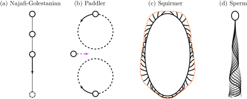
Figure 1: Swimming techniques in inertialess flows that are examined in this study. Conceptual swimmers may comprise sliding spheres that have simple kinematics, such as (a) the collinear motion of the Najafi-Golestanian swimmer and (b) paddling motion. These swimmers can provide insight into more complex biological systems ⁹. (c) Ciliates beat many surface cilia in a coordinated fashion. This is often modeled mathematically with envelope methods, either as a small perturbation to the cell morphology (dashed), or through a surface slip velocity. (d) Sperm, an archetypal “monoflagellate pusher”, propagate a bending wave down a single flagellum, shown here in a time-lapse manner.

2 Mathematical modeling

2.1 Fluid mechanics of microscopic swimming

Newtonian fluid modeling has provided important insights into the mechanisms underlying viscous propulsion. However, the need for detailed study of non-Newtonian swimming has long been recognized ²⁹, ³⁰, and experimental observations of sperm in methylcellulose medium suggest ³¹ that non-Newtonian effects may be important. We will adopt a continuum approach to modeling swimming in biological fluids, as used in for instance Lauga ²⁰, Fu et al. ²¹, Teran et al. ²³, Zhu et al. ²², whereby the nanoscale structure of suspended polymers has been averaged into bulk flow properties.

At microscopic length-scales, viscous forces dominate inertia. We will examine microscopic swimmers in inertialess generalized Stokes flow ³². The equations governing the dynamics of such flow are

$$\nabla\cdot\left(2\mu_{\mathrm{eff}}(\dot{\gamma})\boldsymbol{\varepsilon}(\mathbf{u})\right)-\nabla p+\mathbf{F}=0,\quad\nabla\cdot\mathbf{u}=0,$$ (1)

for $\mathbf{u}$ the fluid velocity field, $\mu_{\mathrm{eff}}$ the effective, or apparent, viscosity of the flow, $p$ the pressure, $\mathbf{F}$ any body forces and $\boldsymbol{\varepsilon}(\mathbf{u})=(\mathbf{\nabla}\mathbf{u}+\mathbf{\nabla}\mathbf{u}^{T})/2$, the strain rate tensor.

A model of shear-thinning polymer suspensions is given by the four-parameter Carreau constitutive law ³³

$$\mu_{\mathrm{eff}}^{\mathrm{car}}(\dot{\gamma})=\mu_{\infty}+(\mu_{0}-\mu_{\infty})(1+(\lambda\dot{\gamma})^{2})^{(n-1)/2},\quad 0<n\leq 1,$$ (2)

for shear rate $\dot{\gamma}=\left(2\varepsilon_{ij}(\mathbf{u})\varepsilon_{ij}(\mathbf{u})\right)^{1/2}$. The effective viscosity $\mu_{\mathrm{eff}}$ of the flow decreases monotonically between a zero shear viscosity, $\mu_{0}$, and an infinite shear viscosity $\mu_{\infty}$. As the time parameter $\lambda$ increases, lower shear rates are required to thin the fluid.

For swimmers with prescribed strokes, a characteristic velocity is given by $U=\omega L$, where $\omega$ is the angular frequency of the swimmer’s stroke and $L$ is a characteristic length, for instance the length of the flagellum. Upon substitution of the viscosity (2) into equations (1) and non-dimensionalizing, we derive the dimensionless equations,

$$\hat{\nabla}\cdot\left[2\left(1+\left[\frac{\mu_{0}}{\mu_{\infty}}-1\right]\left[1+\left(\lambda\omega\hat{\dot{\gamma}}\right)^{2}\right]^{(n-1)/2}\right)\hat{\boldsymbol{\varepsilon}}({\hat{\mathbf{u}}})\right]-\hat{\nabla}\hat{p}+\hat{\mathbf{F}} =0,$$ (3a)

$$\hat{\nabla}\cdot\hat{\mathbf{u}} =0.$$ (3b)

Thus, for swimmers exhibiting prescribed beat kinematics, trajectories are dependent only on three dimensionless quantities: the viscosity ratio $\mu_{0}/\mu_{\infty}$, the power-law index $n$ and the shear index $\mathrm{Sh}=\lambda\omega$ (referred to as $\mathrm{De}$ by Montenegro-Johnson et al. ²⁸). The parameter $\mathrm{Sh}$ has the physical interpretation of the ratio of the fluid’s time parameter to the swimmer’s beat period. Newtonian flow is recovered if any of $\mu_{0}/\mu_{\infty}=1,n=1$ or $\mathrm{Sh}=0$.

This non-dimensionalization reduces the number of free parameters from four to three. In contrast, Newtonian flow arising from prescribed boundary motion has no free parameters. As such, the trajectories of swimmers with prescribed kinematics in Newtonian Stokes flow exhibit no dependency on the absolute value of the viscosity. These values only become important when considering the magnitude of the forces on the swimmer.

When prescribing the kinematics of a swimming stroke, it is convenient to employ the swimmer’s intrinsic ‘body frame’ ³⁴, in which its body neither rotates nor translates. The configuration and deformation of the swimmer are specified by a mathematical function relative to the body frame, and these are transformed into the global ‘lab frame’ coordinates in which we solve the governing equations. This transformation entails use of the a priori unknown translational velocity $\mathbf{U}$ and angular velocity $\mathbf{\Omega}$ of the swimmer. The swimming velocities $\mathbf{U}$ and $\mathbf{\Omega}$ result from the swimmer’s body frame kinematics at any particular time, and are constrained by the conditions that zero net force ³⁵ and torque ³⁶ act on the swimmer. A schematic showing the relationship between the body and lab frames is shown in figure 2a, along with the computational domain used for this study (figure 2b).

It is well-known that in two-dimensional, inertialess Newtonian flow, no solution is possible for the flow arising from translating rigid bodies in unbounded fluid domains. This is known as Stokes’ Paradox, and arises because the flow resulting from a point force in two dimensions diverges as $\log r$ far from the force ³⁷. However, the swimmers we will model are force-free; no net forces or torques act upon them. Furthermore, since we model swimmers in channels, the far-field decays at least as quickly as $\mathcal{O}(1/r)$. Many cells swim close to boundaries, so that finite domain modeling can be used to give a faithful representation of their environment. It is highly instructive ²³, ³⁸, ³⁹ to consider two-dimensional flow models of swimming and thus we will present results for swimmers in finite, two-dimensional domains.

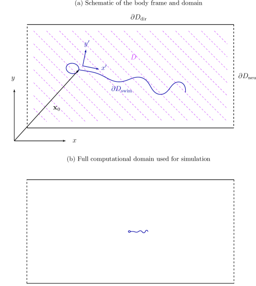
Figure 2: (a) A schematic of the fluid domain $D$ containing a model human sperm $\partial D_{\mathrm{swim}}$, showing no-slip channel walls $\partial D_{\mathrm{dir}}$ and open boundaries $\partial D_{\mathrm{neu}}$. The relationship between the lab frame, $(x,y)$ and the body frame, $(x^{\prime},y^{\prime})$ is also shown, where the body frame origin $\mathbf{x}_{0}$ is a fixed point on the swimmer. Femlets are distributed along the boundary $\partial D_{\mathrm{swim}}$, shown here as a sperm head and flagellum. (b) The full computational domain used in this study. The domain and swimmer are shown to scale.

2.2 The method of femlets

In order to solve microscopic swimming problems in fluids with shear dependent viscosity, the method of femlets was developed by Montenegro-Johnson et al. ²⁸. Drawing inspiration from the method of regularized stokeslets ³ and the Immersed Boundary Method ⁴⁰, ⁴¹, the method of femlets represents the interaction of the swimmer with the fluid through a set of concentrated ‘blob’ forces of unknown strength and direction, with spatial variation prescribed by a cut-off function (figure 3). While the method of regularized stokeslets reduces the problem to finding the coefficients in a linear superposition of velocity solutions of known form, the method of femlets proceeds by applying the finite element method to solve for the fluid velocity field and strength and direction of the forces simultaneously.

For a one-dimensional filament of length $L$ and centerline parameterization $\boldsymbol{\xi}(s,t)$, the force exerted by the filament on the fluid is given by

$$\mathbf{F}(\mathbf{x},t)=\int_{0}^{L}\delta(\mathbf{x}-\boldsymbol{\xi}(s,t))\mathbf{f}(s,t)\,\mathrm{d}s,$$ (4)

where $\mathbf{f}(s,t)$ is a force per unit length determined by the swimmer’s velocity. In the method of femlets, we discretize equation (4) by a set of regularized forces

$$\mathbf{F}(\mathbf{x},t)\approx\sum_{k=1}^{N}g^{\sigma_{x},\sigma_{y}}\left\{\mathbf{R}(s_{k})\cdot[\mathbf{x}-\boldsymbol{\xi}(s_{k})]\right\}\mathbf{f}(s_{k}).$$ (5)

The rotation $\mathbf{R}(s_{k})$ is chosen such that the axis $\mathbf{R}(s_{k})\cdot[\mathbf{x}-\boldsymbol{\xi}(s_{k})]=(x_{k}^{\mathrm{loc}},y_{k}^{\mathrm{loc}})^{T}$ is aligned locally to the swimmer’s tangent at the location of each femlet, and $\sigma_{x},\sigma$ are anisotropic regularization parameters. For this study, we choose an elongated Gaussian cut-off function, as in Montenegro-Johnson et al. ²⁸,

$$g^{\sigma_{x},\sigma_{y}}\{\mathbf{x}^{\mathrm{loc}}\}=\exp\left\{-\left[\frac{(x^{\mathrm{loc}})^{2}}{2\sigma^{2}_{x}}+\frac{(y^{\mathrm{loc}})^{2}}{2\sigma^{2}_{y}}\right]\right\}.$$ (6)

The regularization parameter $\sigma_{x}$ is chosen to give a smooth representation along the swimmer of the force (figure 3b), while reducing $\sigma_{y}$ produces a closer approximation to a line force (equation (4)). A validation of the method of femlets is provided in appendix A.

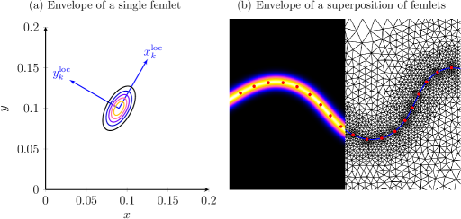
Figure 3: The envelope function of the force exerted by the flagellum on the fluid. The function is approximately zero in the black regions, and increases as the colors lighten. (a) An example elongated femlet cut-off function, given by a two-dimensional elongated Gaussian, oriented by a coordinate transform to align locally with the swimmer’s body. (b) A plot showing the smooth force distribution envelope generated by a sum of such cut-off functions when projected on a finite element mesh; femlet centroids are marked by dots.

We will model swimmers in the truncated channel $D$ shown in figure 2. On the channel walls $\partial D_{\mathrm{dir}}$ we specify Dirichlet velocity conditions, for example the no-slip condition $\mathbf{u}_{\mathrm{dir}}=\mathbf{0}$, and at the truncated boundary $\partial D_{\mathrm{neu}}$ we apply the zero normal stress condition $\boldsymbol{\sigma}\cdot\mathbf{n}=\mathbf{0}$. The swimmer $\partial D_{\mathrm{swim}}$ is not a Dirichlet boundary, but rather a manifold of points within $D$ on which we specify the swimmer’s body frame velocity. This is where the femlets are distributed.

For the two-dimensional problem, $2$ degrees of freedom are associated with each femlet $k$, the lab frame force of the femlet in the $x$ and $y$ directions $(f_{1k},f_{2k})$. This produces $2N_{f}$ additional scalar variables. To calculate the $2N_{f}$ force unknowns, we enforce $2N_{f}$ constraints in the form of Dirichlet velocity conditions $\mathbf{u}_{s}$ given by the swimmer’s velocity in the body frame and applied at the location of each femlet.

3 Results and analysis

3.1 Sliding sphere swimmers

In the results that follow, the fluid domain is given by a channel of length $10L$ and height $5L$, where $L$ is a characteristic length for the swimmer, normalized here to $L=1$ unit. To ensure the independence of the results from the truncation length of the channel, swimmers were also tested in a channel of length $20L$.

We will begin by examining the effects of shear-thinning rheology on a class of model viscous swimmers comprising sliding collinear spheres that oscillate out of phase. The first such swimmer was proposed by Najafi and Golestanian ⁸; it is formed of three spheres which move with the four-stage beat pattern shown in figure 4. The kinematics of the beat is divided into two “effective” strokes, during which the swimmer travels in the direction of net progress, and two “recovery” strokes, during which the swimmer readjusts its configuration to reinitiate an effective stroke. Whilst performing a recovery stroke, the swimmer moves in the opposite direction to the direction of net progress.

We refer to the swimmer’s “progress” as the distance it travels over an effective stroke, “regress” as the distance it travels over a recovery stroke. The swimmer’s “net progress” is the distance travelled over an entire beat cycle. The net progress can be seen as the sum of the distances travelled over all effective strokes minus the sum of the distances travelled over all recovery strokes. In other words,

$$\mbox{net progress}=\sum_{i=1}^{N_{\mathrm{eff}}}\mbox{progress}_{i}-\sum_{i=1}^{N_{\mathrm{rec}}}\mbox{regress}_{i}$$ (7)

for $N_{\mathrm{eff}},N_{\mathrm{rec}}$ the number of effective and recovery strokes respectively.

Figure 4 shows that at any instant, the swimmer can be thought of as comprising a propulsive element and a drag-inducing “payload” element. By force balance, leftward relative motion of an outer sphere results in rightward motion of the remaining spheres through the fluid, and vice-versa. The principle underlying the propulsion of collinear sphere swimmers is that the total drag on the two payload spheres is reduced if they are brought closer together. Thus, the swimmer shown in figure 4 will exhibit overall leftward progress.

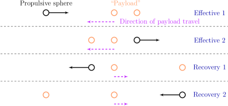
Figure 4: A complete beat cycle of the Najafi-Golestanian swimmer showing the position of the outer spheres relative to the central sphere, the direction in which the propulsive sphere moves (solid arrow) relative to the payload, and the direction and magnitude of swimming (dashed arrow).

Montenegro-Johnson et al. ²⁸ found that a version of the Najafi-Golestanian swimmer with smoothed kinematics progressed more rapidly through shear-thinning fluid. However, the physics behind this enhanced progression were not apparent. We will now consider the simpler original Najafi-Golestanian swimmer, for which the outer spheres move at constant speed during each portion of the four-stage beat cycle shown in figure 4. The body frame positions of the three spheres $i=1,2,3$ are given as a function of time $t$ in table 1, where $d=0.5,a=0.25$ in our model.

Najafi-Golestanian swimmer
Stroke	$x_{1}$	$x_{2}$	$x_{3}$	time $t$
Eff $1$	$-(d+a)+8at$	$0$	$d-a$	$[0,1/4)$
Eff $2$	$-(d-a)$	$0$	$d-a+8a(t-1/4)$	$[1/4,1/2)$
Rec $1$	$-(d-a)-8a(t-1/2)$	$0$	$d+a$	$[1/2,3/4)$
Rec $2$	$-(d+a)$	$0$	$d+a-8a(t-3/4)$	$[3/4,1)$

Table 1: The body frame positions of the three spheres of the Najafi-Golestanian swimmer we will model, for $d=0.5,a=0.25$, over each portion of its beat cycle.

Figure 5 shows the effects of shear-thinning rheology upon the Najafi-Golestanian swimmer for varying power-law index $n$. As $n$ is decreased from the Newtonian case $n=1$, the swimmer’s progress over its effective strokes (figure 5a) and regress over recovery strokes (figure 5b) are both decreased. At all moments during its beat cycle, the swimmer swims more slowly in shear-thinning fluid. This effect is slight: for $n=0.5$, the swimmer’s speed is approximately $3\%$ lower during the effective strokes and $5\%$ lower during the recovery strokes than for $n=1$ (Newtonian fluid). However, since swimming velocity is reduced more during the recovery strokes, the result is in fact an increase in net progress, shown in figure 5c. This behavior is demonstrated in figure 6, which shows the position of the swimmer over five complete beat cycles in Newtonian and shear-thinning fluid.

Figure 5: The effects of shear-thinning on the Najafi-Golestanian swimmer with the four-stage beat pattern given in table 1. (a) The progress during each effective stroke and (b) the regress during each recovery stroke as functions of the power-law index $n$. Since the decrease in regress is greater for $n<1$, the overall effect of shear-thinning is an increase in net progress as $n$ decreases (c). In each panel, the case corresponding to Newtonian fluid is marked in lighter gray (orange online).

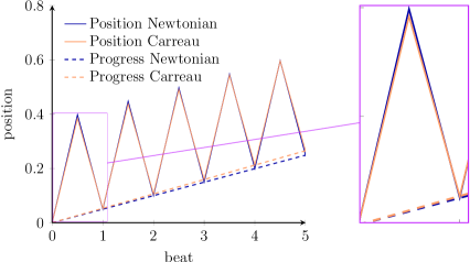
Figure 6: Simulation results of the position of the Najafi-Golestanian swimmer over five beat cycles, demonstrating how decreasing the instantaneous swimming speed at all times in shear-thinning fluid can lead to an increase in overall progress, provided swimming speed is decreased more during the recovery stroke. The rheological parameters of the Carreau fluid are $\mu_{0}/\mu_{\infty}=2,n=0.5$ and $\mathrm{Sh}=1$.

The swimmer’s progress and regress are reduced by shear-thinning, but regress is reduced more and hence overall progress is increased. But what is responsible for this decrease in instantaneous swimming speed, and why is this effect enhanced during the recovery stroke?

Figure 7 shows the effective viscosity of the fluid surrounding the swimmer at time $t=0$ for rheological parameters $\mu_{0}/\mu_{\infty}=2,n=0.5$ and $\mathrm{Sh}=1$. The effective viscosity of the fluid surrounding the propulsive sphere is significantly lower than that surrounding the payload. In the lab frame, the propulsive sphere moves more quickly than the payload, thereby thinning the surrounding fluid to a greater extent.

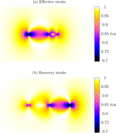
Figure 7: The effective viscosity of Carreau fluid, normalized to $\mu_{0}=1$, surrounding the Najafi-Golestanian swimmer (table 1) at (a) the start of effective stroke $1$ and (b) the start of recovery stroke $2$ for $\mu_{0}/\mu_{\infty}=2,n=0.5$ and $\mathrm{Sh}=1$. The fluid around the propulsive sphere is thinner than that around the payload.

The drag on a sphere moving in inertialess Newtonian fluid is proportional to the viscosity of the fluid. Whilst Carreau fluid is non-Newtonian, this observation is key to understanding the effects of shear-thinning rheology. If fluid is relatively thicker around the payload spheres, the resistance coefficient of those spheres will be relatively higher than that of the propulsive sphere. Thus, the instantaneous velocity of the swimmer will be reduced.

We examine this effect by calculating the average viscosity of the flow at points on a small circle, of radius $\epsilon$ say, surrounding each sphere $i$ centered at $(x_{i},y_{i})$

$$\bar{\mu}_{i}=\bar{\mu}_{\mathrm{eff}}(\dot{\gamma}(\mathbf{u}(r_{i}))),$$ (8)

for $r_{i}$ coordinates $(x,y)$ such that $(x-x_{i})^{2}+(y-y_{i})^{2}=\epsilon^{2}$. The average for each sphere is calculated from $20$ azimuthal coordinates. We then split the set of viscosities into the viscosities of the fluid surrounding propulsive $\mu^{\mathrm{prop}}_{i}$ and drag-inducing payload $\mu^{\mathrm{drag}}_{i}$ spheres. We then calculate the “viscosity differential”

$$\mu_{\mathrm{diff}}=\frac{1}{N_{\mathrm{prop}}}\sum_{i=1}^{N_{\mathrm{prop}}}\mu^{\mathrm{prop}}_{i}-\frac{1}{N_{\mathrm{drag}}}\sum_{i=1}^{N_{\mathrm{drag}}}\mu^{\mathrm{drag}}_{i},$$ (9)

for $N_{\mathrm{prop}}$ and $N_{\mathrm{drag}}$ the number of propulsive and drag-inducing spheres respectively. For the Najafi-Golestanian swimmer, $N_{\mathrm{prop}}=1$ and $N_{\mathrm{drag}}=2$, and the propulsive and payload spheres change according to the portion of the beat cycle, as demonstrated in figure 4. The decrease in the Najafi-Golestanian swimmer’s instantaneous velocity is shown as a function of the viscosity differential (9) in figure 8.

At time $t=0$, the swimmer initiates an effective stroke. The velocity of the swimmer at $t=0$, relative to the Newtonian case, is shown as a function of $\mu_{\mathrm{diff}}$ in figure 8a, for varying $n$ (light gray, orange online), $\mu_{0}/\mu_{\infty}$ (dark gray, blue online) and $\mathrm{Sh}$ (medium gray, magenta online). This figure shows that the result of varying these parameters is approximately equivalent with respect to the viscosity differential. Furthermore, figure 8a demonstrates that the reduction in velocity arising from shear-thinning rheology is approximately proportional to the viscosity differential. This proportionality is to be expected, because the the drag coefficients of the spheres are approximately proportional to the viscosity of the fluid surrounding them.

However, the coefficient of proportionality between the relative instantaneous velocity and the viscosity differential is greater during the recovery stroke (figure 8b). This increase entails that the velocity is decreased more during the recovery stroke, and must arise not from the viscosity at the surface of the spheres, but in some way from the rate at which the viscosity field increases away from each sphere.

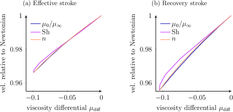
Figure 8: The velocity relative to the Newtonian case of the Najafi-Golestanian swimmer when initiating an effective stroke (a) and a recovery stroke (b) as a function of the viscosity differential $\mu_{\mathrm{diff}}$. The velocity has been calculated while varying the three rheological parameters of Carreau flow for $n=0.5,\mu_{0}/\mu_{\infty}\in[1,2],\mathrm{Sh}=0.5$ (dark gray, blue online), $n=0.5,\mu_{0}/\mu_{\infty}=2,\mathrm{Sh}\in[0,0.5]$ (medium gray, magenta online) and $n\in[0.5,1],\mu_{0}/\mu_{\infty}=2,\mathrm{Sh}=0.5$ (light gray, orange online). This figure demonstrates an apparent proportionality between the velocity and the viscosity differential, and that the viscosity differential is enhanced during the recovery stroke.

These results raise three interesting questions: (1) is the viscosity differential always negative, reducing instantaneous velocity, for three-sphere swimmers, (2) will the coefficient of proportionality between the instantaneous velocity and the viscosity differential always be greater during the recovery stroke and (3) how does the rate at which viscosity increases away from the swimmer affect progress? To answer these questions, we will first consider a morphologically identical three-sphere swimmer with different beat kinematics.

3.2 A three-sphere “paddler”

Drescher et al. ⁴² showed that the far-field flow induced by the the biflagellate green alga Chlamydomonas Reinhardtii may be approximated by three stokeslets: two outer stokeslets exerted a backwards force, representing the flagella, balanced by a central stokeslet, representing the cell body. Inspired by this approximation, one could consider a paddling three-sphere swimmer ⁹ exhibiting the kinematics shown in figure 9a.

The central sphere is stationary in the body frame, and represents the swimmer’s body, or payload. The two outer spheres move along closed, non-intersecting curves in the same plane as the body, such that these curves are a mirror image of one another. The behavior of this swimmer in Newtonian fluid was analyzed by Polotzek and Friedrich ⁹; it was shown that the direction the swimmer travels is dependent upon the loci of the outer swimming spheres.

We will consider a swimmer for which the swimming spheres move along rectangles, centered in line with body sphere. The effective stroke occurs when the outer spheres are nearer the body, so that the swimmer shown in figure 9a will generate a net displacement downwards. Since no net motion of the swimmer occurs whilst the swimming arms are moving directly towards or away from one another, we may consider only the two parts of the stroke given in table 2.

Three sphere paddler
Stroke	$(x_{1},y_{1})$	$(x_{2},y_{2})$	$(x_{3},y_{3})$	time $t$
Rec	$d-4dt,y_{\mathrm{rec}}$	$0,0$	$d-4dt,-y_{\mathrm{rec}}$	$[0,1/2)$
Eff	$-d+4d(t-1/2),y_{\mathrm{eff}}$	$0,0$	$-d+4d(t-1/2),-y_{\mathrm{eff}}$	$[1/2,1)$

Table 2: The body frame positions of the three spheres for the paddling swimmer over the effective and recovery stroke, where in our model $d=0.5,y_{\mathrm{rec}}=0.75$ and $y_{\mathrm{eff}}=0.25$.

For $d=0.5,y_{\mathrm{rec}}=0.75$ and $y_{\mathrm{eff}}=0.25$, figures 9b and 9c show the swimmer’s progress and regress over its effective and recovery strokes respectively. In contrast to the Najafi-Golestanian swimmer considered above, shear-thinning increases the instantaneous swimming speed of this paddler. Progress is increased by around $1\%$, and regress by around $2\%$. The result is a decrease in net progress (figure 9d). Thus, despite swimming more quickly at all times, this swimmer is hindered by shear-thinning flow. This behavior is demonstrated in figure 10, which shows the position of the swimmer over five complete beat cycles in Newtonian and shear-thinning fluid.

As with the Najafi-Golestanian swimmer, the effect of shear-thinning is small for the parameters considered. However, these effects are sensitive to kinematics. The Najafi-Golestanian swimmer and the paddler both comprise three sliding spheres, but through their kinematics they are affected by shear-thinning in opposite manners.

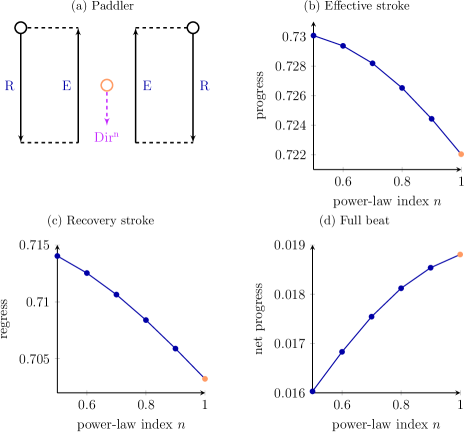
Figure 9: The effects of shear-thinning on the paddler (a) with the two-stage beat pattern given in table 2. During the portions of the beat represented by the dashed black lines, the swimmer does not progress and as such they are not considered here. The dashed arrow shows the swimming direction. (b) The progress during the effective stroke and (c) the regress during the recovery stroke as functions of the power-law index $n$. The greater increase in regress results in a decrease in net progress with shear-thinning rheology, (d). In each panel, the case corresponding to Newtonian fluid is marked in lighter gray (orange online).

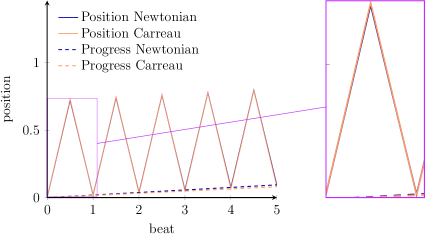
Figure 10: Simulation results of the position of the paddler over five beat cycles, demonstrating how increasing the instantaneous swimming speed at all times in shear-thinning fluid can lead to an decrease in net progress, provided swimming speed is decreased more during the recovery stroke. The observed effect is exactly opposite to that of the Najafi-Golestanian swimmer, summarized in figure 6. The rheological parameters of the Carreau fluid are $\mu_{0}/\mu_{\infty}=2,n=0.5$ and $\mathrm{Sh}=1$.

To balance the forces induced by the two propulsive spheres, the lab frame velocity of the drag-inducing sphere is greater than the lab frame velocity of the propulsive spheres. Thus in shear-thinning flow, fluid will be relatively thinner around the drag-inducing sphere than around the propulsive spheres (figure 11). Accordingly, the viscosity differential for this swimmer is positive, in contradistinction to the Najafi-Golestanian swimmer above, and thus the swimmer’s instantaneous velocity is increased by shear-thinning rheology. But why is this effect enhanced during the recovery stroke when the spheres are further apart?

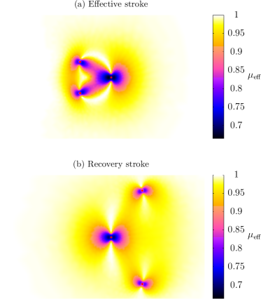
Figure 11: The effective viscosity of Carreau fluid, normalized to $\mu_{0}=1$, surrounding the paddler (table 2) at (a) the start of the effective stroke and (b) the start of the recovery stroke for $\mu_{0}/\mu_{\infty}=2,n=0.5$ and $\mathrm{Sh}=1$. The fluid around the propulsive sphere is thinner than that around the payload.

Figure 12 shows the velocity of the swimmer relative to the Newtonian case as a function of the viscosity differential at a moment during an effective stroke (figure 12a) and a recovery stroke (figure 12b). During the recovery stroke, the velocity relative to the Newtonian case is again approximately proportional to the viscosity differential. The constant of proportionality is approximately half that for the Najafi-Golestanian swimmer (figure 8), which may be because there are twice as many propulsive elements.

However, this proportionality fails during the effective stroke, when the spheres are close to one another. Each sphere thins a significant region of fluid, and these regions overlap substantially, decreasing the effect of the viscosity differential. This decrease is apparent when considering the shear-index data in figure 12a. For low values of $\mathrm{Sh}$, high shear is required to thin the flow. Thus, the viscosity fields generated by the spheres that comprise the swimmer do not interact, and the proportionality between the viscosity index and the increase in velocity is equal to that during the recovery stroke (figure 12b), for which the spheres are further apart. When the value of $\mathrm{Sh}$ increases past a critical value, despite increases in the viscosity differential velocity is in fact decreased. After a further critical value, the viscosity differential is in fact decreased by increasing $\mathrm{Sh}$.

The envelope of thinned fluid surrounding the swimmer during the effective stroke inhibits its progress. Increasing the shear index past the optimum increases the size of this envelope, further hindering swimming. This result is consistent with the existence of an optimum value of $\mathrm{Sh}$ for the progress of the Najafi-Golestanian swimmer considered by Montenegro-Johnson et al. ²⁸.

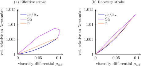
Figure 12: The velocity relative to the Newtonian case of the paddler at the commencement of (a) an effective stroke and (b) a recovery stroke as functions of the viscosity differential $\mu_{\mathrm{diff}}$. The velocity has been calculated while varying the three rheological parameters of Carreau flow for $n=0.5,\mu_{0}/\mu_{\infty}\in[1,2],\mathrm{Sh}=0.5$ (dark gray, blue online), $n=0.5,\mu_{0}/\mu_{\infty}=2,\mathrm{Sh}\in[0,0.5]$ (medium gray, magenta online) and $n\in[0.5,1],\mu_{0}/\mu_{\infty}=2,\mathrm{Sh}=0.5$ (light gray, orange online). During the recovery stroke (b), spheres are far apart and there is approximate proportionality between the increase in velocity and the viscosity differential. During the effective stroke (a), however, interactions between the viscosity fields of the spheres reduce the effect of the viscosity differential. For low values of $\mathrm{Sh}$ (medium gray, magenta online), more shear is required to thin the flow. Thus, proportionality between velocity increase and viscosity differential is maintained with the same constant for effective and recovery strokes due to decreased viscosity field interactions.

Thus, in the limit of large separation between spheres, the envelopes of thinned fluid surrounding each sphere do not interact, and instantaneous velocity is approximately proportional to the viscosity differential. If spheres are close enough to generate an envelope of thinned fluid surrounding the whole swimmer, that envelope hinders swimming, reducing the constant of proportionality between swimming velocity and the viscosity differential. To examine the effects of the envelope of thinned fluid further, we will now consider squirming models of ciliates.

3.3 Slip velocity squirmers

Much like sphere swimmers, cilia utilized for locomotion typically beat with an asymmetric effective-recovery stroke pattern ⁴³. They perform an effective stroke when fully extended, moving through the fluid perpendicular to their centerline, and then recover by moving tangentially to their centerline (figure 13).

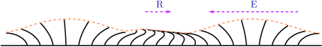
Figure 13: A schematic of a ciliated surface. Cilia beat with an effective-recovery stroke pattern, marked with E and R respectively, pushing fluid locally in the direction shown. The cilia are activated in a coordinated, metachronal fashion. The envelope of this motion is given by the dashed green line.

Ciliated swimmers generally express a large number of cilia which beat with a phase difference between neighbors ⁴⁴. Examples are the protozoa Opalina and Paramecium ⁴⁵ and the alga Volvox Carteri. This type of swimming motivates ‘envelope’ modeling approaches ⁴⁶ whereby the array of cilia are represented by either a slip velocity condition on the cell surface, or by small ‘squirming’ deformations of the cell body ⁴⁷, ⁴⁸.

We will analyze a model swimmer with a time independent stroke, the effects of coordinated ciliary beating being time averaged over a beat as a constant slip velocity. The tangential slip velocity is typically decomposed into ‘swimming modes’ of spherical harmonics ⁴⁹

$$u_{\theta}(\theta)=\sum_{n=1}^{\infty}\alpha_{n}K_{n}(\cos\theta),$$ (10)

for

$$K_{n}(\cos\theta)=\frac{(2n+1)\sin\theta}{n(n+1)}L_{n}^{\prime}(\cos\theta),$$ (11)

with $L_{n}(\cos\theta)$ the $n$-th Legendre polynomial. Thus, slip velocity squirmers are characterized by the coefficients $\alpha_{n}$ of the modes of their swimming.

The simplest two-dimensional squirmer has a single mode, i.e. $\alpha_{n}=0$ for all $n\geq 2$. This ‘treadmilling’ squirmer has a radius $r=L/2$ and generates a time independent tangential slip velocity in the body frame of

$$u_{\theta}=(1/2)\sin\theta\ \mbox{on}\ r=L/2.$$ (12)

A treadmilling squirmer is shown alongside an image of Volvox Carteri, in figure 14. Since swimmer kinematics and the fluid domain are symmetric about the line $y=0$, the squirmer swims purely in the positive $x$ direction.

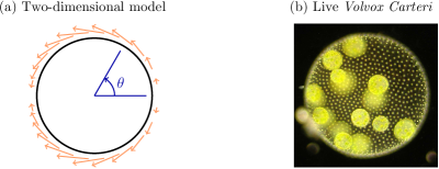
Figure 14: (a) A schematic of a two-dimensional treadmilling squirmer, along with (b) a micrograph of a Volvox Carteri colony, showing surface cilia that beat in a coordinated fashion to propel the colony forwards. This cell also shows a number of characteristic ‘daughter’ colonies within it. Image taken by Prof. Raymond E. Goldstein, University of Cambridge.

Shear-thinning decreases the velocity of this squirmer (figure 15). This result draws an interesting parallel with the work of Zhu et al. ²², who found that spherical squirmers were also hindered by a different non-Newtonian fluid property, viscoelasticity. Figure 15c shows a striking apparently linear dependence of the swimming velocity upon the power-law index $n$. The decrease in velocity is small; for $\mu_{0}/\mu_{\infty}=2,n=0.5$ and $\mathrm{Sh}=1$, the velocity is reduced by a little over $3\%$.

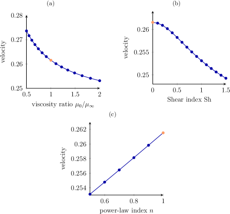
Figure 15: The velocity of the treadmilling squirmer with slip velocity given by equation (12) as a function of (a) the viscosity ratio $\mu_{0}/\mu_{\infty}$ with $n=0.5$ and $\mathrm{Sh}=1$, (b) the shear index $\mathrm{Sh}$ with $n=0.5$ and $\mu_{0}/\mu_{\infty}=2$ and (c) the power-law index $n$ with $\mu_{0}/\mu_{\infty}=2$ and $\mathrm{Sh}=1$. In each panel, the case corresponding to Newtonian fluid is marked in lighter gray (orange online).

The effective viscosity field of the flow has a simple form; even relatively near to the swimmer, contours of equi-viscosity are approximately circular, centered on the swimmer (figure 16). However, very near to the surface, the fluid surrounding the propulsive elements of the treadmilling squirmer is relatively thicker than that surrounding the drag-inducing portions. Thus, the viscosity differential for this squirmer is positive, yet its velocity is decreased by shear-thinning, demonstrating that slip velocity models differ from no-slip multiple sphere swimmers in this respect. The reduction in velocity arises from the envelope of thinned fluid surrounding the squirmer.

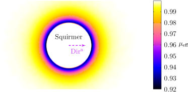
Figure 16: The effective viscosity $\mu_{\mathrm{eff}}$ of Carreau fluid, normalized to $\mu_{0}=1$, surrounding the treadmilling squirmer for $\mu_{0}/\mu_{\infty}=2,n=0.5$ and $\mathrm{Sh}=0.5$. These parameter values are the extremal values used for the data in figures 17 and 18. Away from the swimmer surface, contours of equi-viscosity are approximately circular. On the surface, fluid is relatively thicker surrounding the propulsive portions of the swimmer. The squirmer is aligned to the positive $x$-axis, as in figure 14a, and the direction of travel is indicated by the dashed arrow.

Figure 17 shows the radial variation in the effective viscosity of the fluid surrounding the squirmer. As $n$ decreases, the viscosity immediately surrounding the swimmer decreases, but the rate at which the viscosity approaches the zero-shear value increases. As a result of this increase, the size of the envelope of thinned fluid surrounding the swimmer varies little with changes in rheological parameters (figure 17a). For any fixed value of the radial coordinate $r$, with $r=0.5$ being the squirmer’s surface, the effective viscosity at that point decreases approximately linearly with $n$ (figure 17b).

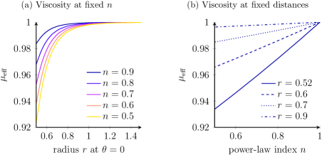
Figure 17: The effective viscosity of the fluid envelope surrounding the treadmilling squirmer. (a) Changes in the viscosity field as a function of the radial coordinate $r$ for different values of the power-law index $n$. The swimmer surface is given by $r=0.5$. (b) For fixed values of $r$, the effective viscosity exhibits a near linear dependence upon the power-law index $n$.

Since the decrease in swimming velocity also exhibits a linear dependence upon the power-law index $n$, we examine the dependence of swimming velocity on the effective viscosity of the fluid surrounding the squirmer. Figure 18a shows the decrease in swimming velocity relative to the Newtonian case as a function of the effective viscosity of the fluid envelope at $r=0.52$, a small distance from the squirmer’s surface, for varying viscosity ratio, shear index and power-law index. This figure demonstrates a strong linear correlation between the effective viscosity of the fluid a small distance from the swimmer’s surface and the swimmer’s velocity.

However, whilst the absolute values of viscosity do not affect swimmers with prescribed kinematics, the envelope of thinned fluid shields the far field flow from the flow generated by the squirmer. As fluid becomes relatively thinner around the squirmer, the decay rate of the near-field flow increases. This draws an interesting parallel with the work of Zhu et al. ²², who found a similar effect for viscoelastic (Giesekus) fluids. In the near-field, along the line $\theta=0$, the velocity of the flow is approximately

$$u\approx\frac{A}{r^{\alpha}},\quad\therefore\log u\approx\log A-\alpha\log r.$$ (13)

Thus, the flow decay rate is given by

$$\alpha=-\frac{\Delta\log u}{\Delta\log r}.$$ (14)

Close to the squirmer’s surface, the Newtonian flow decay rate $\alpha_{\mathrm{newt}}=1.95$.

Figure 18b shows the swimming velocity of the squirmer as a function of this decay rate at $r=0.52,\theta=0$, a small distance from the squirmer’s surface, relative to the Newtonian case for varying rheological parameters $\mu_{0}/\mu_{\infty},n$ and $\mathrm{Sh}$. The decrease in velocity and increase in flow decay exhibit a linear relationship, and are the same magnitude; the slope of the curve is close to $-1$. This observation motivates the following argument: The squirmer generates an envelope of thinned fluid around itself when swimming through Carreau fluid. This envelope increases the decay rate of flow away from the squirmer’s surface. Thus, prescribed motion on the surface moves relatively less fluid, which decreases the swimming velocity.

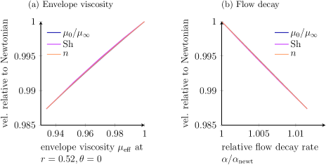
Figure 18: The velocity relative to the Newtonian case of the treadmilling squirmer as a function of (a) the effective viscosity on the contour $r=0.52$ and (b) the rate of decay $\alpha$ of the velocity from the surface of the squirmer relative to the Newtonian case $\alpha_{\mathrm{newt}}$. The velocity has been calculated while varying the three rheological parameters of Carreau flow for $n=0.5,\mu_{0}/\mu_{\infty}\in[1,2],\mathrm{Sh}=0.5$ (dark gray, blue online), $n=0.5,\mu_{0}/\mu_{\infty}=2,\mathrm{Sh}\in[0,0.5]$ (medium gray, magenta online) and $n\in[0.5,1],\mu_{0}/\mu_{\infty}=2,\mathrm{Sh}=0.5$ (light gray, orange online). This figure demonstrates a striking proportionality between the velocity and the decay rate of the fluid.

However, models of squirmers exhibiting surface velocity distribution may neglect effects arising from rheological interactions at the scale of individual cilia. These interactions may be captured more effectively by squirming models for which the surface is subject to small deformations. For many ciliates, such as the protozoa Opalina, surface deformation provides a better representation of the swimmer than slip velocity modeling. It may be that rheologically-enhanced propulsion at the cilium scale is captured by envelope models with surface deformation.

3.4 Monoflagellate pushers

We will now examine the effects of shear-thinning rheology on the swimming of a two-dimensional model sperm with prescribed waveform. Since the trajectories of such swimmers are two-dimensional, we will analyze their shape using variables from Computer Aided Semen Analysis (CASA), see for example Mortimer ⁵⁰. Our usage will differ slightly, in that CASA variables are statistical averages over many beat cycles determined from video microscopy of living cells sampled at a given frequency, whereas we will generate a smooth, time periodic waveform and thus our parameters will be measured over a single beat. The variables we will consider are demonstrated for an example trajectory over one beat cycle in figure 19.

Sperm do not exhibit an effective-recovery stroke pattern, but rather swim by propagating a travelling wave along the flagellum. As such, we now refer to a swimmer’s ‘progress’ as the distance between its start and end points over a beat. We will also consider its straight line velocity $\mathrm{VSL}=\mathrm{progress}/T$ and its curvilinear, or instantaneous, velocity $\mathrm{VCL}$, the velocity of the cell at any given point in time. The amplitude of the cell’s lateral head displacement $\mathrm{ALH}$, is given by the difference between the maximum and minimum $y$ values on the trajectory. We also consider the path length $\mathrm{PL}$ of the trajectory, that is the total distance travelled, as well as the straightness of the path $\mathrm{STR}=\mathrm{progress}/\mathrm{PL}$.

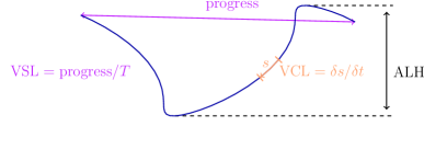
Figure 19: Swimming parameters for the trajectory (dark gray, blue online) of a swimmer moving from right to left over one beat cycle of period $T$. The instantaneous velocity is the derivative of arclength $s$ along the path with respect to time.

The swimmer is propelled by a single flagellum that propagates a bending wave along its length, generating the forces required to move the cell forward. We parameterize the flagellum in terms of its shear angle $\psi(s,t)$ given in the body frame. A shear angle of the form

$$\psi(s,t)=Cs\cos[2\pi(ks-\omega t)],$$ (15)

represents a bending wave propagating down the flagellum, steepening towards the less stiff distal end with a linear envelope. This shear angle produces a waveform representative of sperm swimming in high viscosity fluids ³¹, shown in figure 20. The lab frame position of the flagellum is then given by rotating the centerline in the body frame by the swimmer’s orientation, and translating by the current head position.

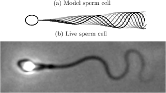
Figure 20: (a) The flagellar waveform generated by shear angle (15) and (b) a micrograph of a human sperm in medium containing $1\%$ methylcellulose, a fluid with comparable viscosity to that of cervical mucus.

Length scales are normalized to the flagellum length, so that one length unit corresponds to $55\,\mu\mathrm{m}$, and one time unit corresponds to a single beat of the flagellum. Thus, for a tail beating at $10\,\mathrm{Hz}$ one time unit corresponds to $0.1\,\mathrm{s}$.

Montenegro-Johnson et al. ²⁸ showed that particular sperm-like swimmer progressed further in shear-thinning fluids. In this study, we will show that this behavior arises for other sperm-like swimmers, and examine the interplay between physical mechanisms and morphological changes in swimming trajectory that cause it.

We will examine the trajectories of swimmers with waveforms generated by the shear angle (15) for maximum shear angle $A=0.45\pi$ and wavenumber $k=2.5$, i.e. $2.5$ waves on the flagellum. We have also examined waveforms produced by other parameter values, and found that the effects of shear-thinning were consistent for all values considered. The cell head will be given by an ellipse of fixed eccentricity, but different area, given in table 3.

Sperm head morphologies
$a_{x}$	$a_{y}$	Area	Circumference
0.045	0.036	0.0016$\pi$	0.255
0.05	0.04	0.002$\pi$	0.284
0.055	0.044	0.0024$\pi$	0.312

Table 3: Elliptical head morphologies of constant eccentricity, but different area scaled with flagellum length, corresponding to the data in figure 22. These morphologies, from top to bottom correspond with dark to light plots.

Figure 21 shows the trajectories of an example sperm for three values of the viscosity ratio. From this figure, it is apparent that shear-thinning increases the progress of sperm-like swimmers significantly; for $\mu_{0}/\mu_{\infty}=4,n=0.5$ and $\mathrm{Sh}=1$, this increase is around $40\%$ over the Newtonian case. However, it is not immediately apparent how much of the increase in progress is associated with increased path straightness ($\mathrm{STR}$) and how much arises from increased instantaneous velocity ($\mathrm{VCL}$).

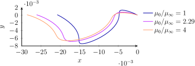
Figure 21: Trajectories of the body frame origin $\mathbf{x}_{0}$, given by the head-flagellum junction, of a two-dimensional sperm-like swimmer in Carreau fluid for different values of the viscosity ratio $\mu_{0}/\mu_{\infty}$, showing an increase in progress and a decrease in $\mathrm{ALH}$ as $\mu_{0}/\mu_{\infty}$ increases.

Figure 22 demonstrates the effects of shear-thinning on the shape of the swimming trajectory for sperm with the three different head sizes given in table 3. The trajectories that these swimmers with different head sizes follow in Stokes flow are shown in figure 22a, showing that increasing head size leads to a small decrease in progress, due to increased drag. Shear-thinning increases progress (figure 22b) by reducing the side-to-side motion of the cell $\mathrm{ALH}$ (figure 22c) but increasing its instantaneous velocity $\mathrm{VCL}$, as reflected by increased path length $\mathrm{PL}$ (figure 22d). This increases the swimmer’s path straightness, $\mathrm{STR}$, shown in figure 22e, which is apparent when the trajectories of a single swimmer, with $a_{x}=0.05$ and $a_{y}=0.04$, for various values of the viscosity ratio are plotted together (figure 21).

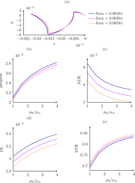
Figure 22: (a) Trajectories of the cells with head morphologies given in table 3, swimming in Stokes flow with $n=0.5$, $\mu_{0}/\mu_{\infty}=4$ and $\mathrm{Sh}=1$. For $n=0.5$ and $\mathrm{Sh}=1$, the effect of varying the viscosity ratio $\mu_{0}/\mu_{\infty}$ on (b) the swimmers’ progress, (c) the amplitude of the swimmers’ lateral head displacement, (d) the path length of the swimmers’ trajectories and (e) the swimmers’ path straightness.

These effects are robust to morphological and kinematic changes. Varying the eccentricity of the cell head or the wavenumber changes the swimmer’s trajectory, but the rheological effects that we show are consistent with changes in these parameters. To understand the increase in cell progress, we will now examine the viscosity field surrounding the swimmer, and the force generated by the flagellum.

The viscosity field surrounding the swimmer is shown for four values of the shear index $\mathrm{Sh}$ in figure 23. Fluid is thickest around the cell head, and there is a gradient of thick to thin fluid along the flagellum, as well as the slightly less obvious feature of a gradient of thick to thin fluid across the swimmer which alternates in sign at local maxima of the shear angle $\psi$. As $\mathrm{Sh}$ is increased to an optimum value these gradients are enhanced, after which they decrease because the fluid becomes thinned substantially at the head end of the flagellum. Montenegro-Johnson et al. ²⁸ found an optimal value of $\mathrm{Sh}$ for a particular sperm-like swimmer’s progress. We now find that this optimal progress is associated with maximal gradients along the flagellum.

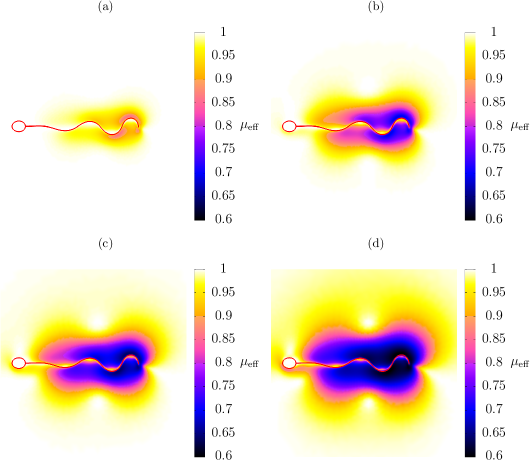
Figure 23: The impact of varying $\mathrm{Sh}=\lambda\omega$ on the effective viscosity $\mu_{\mathrm{eff}}$ of Carreau fluid surrounding a two-dimensional sperm-like swimmer at (a) $\mathrm{Sh}=0.2$, (b) $\mathrm{Sh}=0.8$, (c) $\mathrm{Sh}=1.5$ and (d) $\mathrm{Sh}=3$ with $\mu_{0}/\mu_{\infty}=2$ and $n=0.5$. In these figures, the area of the cell head is $0.002\pi$, the wavenumber $k=2.5$ and the maximum shear angle $A=0.45\pi$.

We examine the forces exerted by the flagellum on the fluid at five equally spaced instants over half its beat cycle for varying viscosity ratio. At each moment, the gradient of thick to thin fluid along the flagellum that arises in shear-thinning fluids entails that forces generated in the proximal (near to head) portion of the flagellum have greater magnitude relative to those in the distal (near to tip) portion, when compared to the Newtonian case (figure 24). Thus, shear-thinning induces a redistribution of force from the distal to the proximal end of the flagellum. This redistribution has the effect of making the force distribution more symmetric about the body axis, and thus straightens the trajectory. This effect is shown in figure 25, where the magnitude and direction of swimming have been plotted for a sperm aligned with the negative $x-$axis at times $t=0,0.1,\dots 0.4$ for changing values of the viscosity ratio. Figure 25 also demonstrates the increase in the magnitude of instantaneous velocity resulting from shear-thinning rheology. The increased instantaneous velocity acts in concert with the straightened path to yield significant increases in progress.

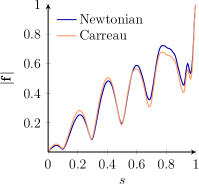
Figure 24: The magnitude of the force that the flagellum exerts upon the fluid at time $t=0$ for Newtonian (dark gray, blue online) and Carreau (light gray, orange online) fluids with $\mu_{0}/\mu_{\infty}=2,n=0.5$ and $\mathrm{Sh}=0.8$, close to the optimal value of $\mathrm{Sh}$ found by Montenegro-Johnson et al. ²⁸.

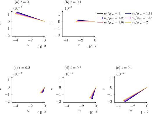
Figure 25: The magnitude and direction of swimming of a sperm oriented in the negative $x$ direction with wavenumber $k=2.5$ and maximum shear angle $A=0.45\pi$ at times $t=0,0.1,0.2,0.3,0.4$, for varying viscosity ratio. These times span half a complete beat cycle. This figure demonstrates that shear-thinning results in straighter swimming and increased instantaneous velocity.

4 Discussion

We have analyzed the effects of shear-thinning rheology on three distinct classes of microscopic swimmer with prescribed kinematics in Carreau fluid. This continuum approach to modeling biological fluids may not be appropriate when the swimmer and the suspended fibers are of a comparable length, as with bacteria in mucus ¹², but it can still provide insight into important effects.

Whilst our modeling is two-dimensional, the observed physical effects are likely to be present for three-dimensional swimmers: sliding spheres exert stresses on the fluid, thereby thinning a surrounding envelope. The Najafi-Golestanian swimmer payload travels more slowly through the fluid than its propulsive sphere. Consequently, fluid surrounding the propulsive sphere is thinned more than fluid surrounding the payload spheres, resulting in a decrease in instantaneous velocity. By contrast, the paddler payload moves more quickly through the fluid than the propulsive elements, fluid around the payload is relatively thinner, thereby increasing instantaneous velocity. The relatively higher decay rate of three-dimensional flow will be associated with an increased decay of the viscosity field around each sphere. This decay will in turn reduce the asymmetry between the effects of shear-thinning on the effective and recovery strokes. So while shear-thinning will decrease both the progress and regress of a Najafi-Golestanian swimmer, we therefore predict that the increase in net progress will be relatively less than for an equivalent two-dimensional swimmer.

The squirmer in three dimensions will again thin an envelope of surrounding fluid, enhancing flow decay rate and thereby decreasing swimming velocity in shear-thinning fluids. For sperm-like swimmers, the prescribed waveforms we considered increase in velocity to the distal portion of the flagellum, and are therefore likely to generate a gradient of thick to thin fluid along the flagellum as in the two-dimensional case. However, in three dimensions, fluid can also pass over the flagellum, and so this gradient may be reduced.

The effects found also give insight into sliding sphere swimmers that may violate Purcell’s Scallop theorem. Since the instantaneous velocity of the sliding sphere swimmers analyzed is approximately proportional to the viscosity differential, an asymmetry between the body frame speed of effective and recovery strokes should allow a reciprocal swimmer to progress through inertialess Carreau fluid. Net progress is made possible because faster motion thins the fluid to a greater extent, thereby inducing an asymmetry between the effective and recovery flow viscosity fields. In Newtonian fluid, no such asymmetry arises, and due to the time independence in the governing equations, such reciprocal motion will not result in net progress.

Two such reciprocal swimmers may be formed from each of the Najafi-Golestanian swimmer and the three-sphere paddler, as shown in figure 26. We refer to these models as the speed-asymmetric collinear swimmer and paddler respectively. For each speed-asymmetric swimmer, a “pusher” and “puller” version of the swimmer may be modeled: pushers are swimmers whose payload is pushed from behind, such as most animal sperm, whereas pullers, such as algae are pulled from the front.

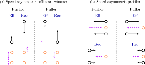
Figure 26: Reciprocal sliding sphere swimmers that cannot progress through inertialess Newtonian fluid, but may progress through inertialess Carreau fluid. These swimmers are pusher and puller versions of (a) the Najafi-Golestanian swimmer and (b) the paddler, showing the effective and recovery strokes with an indication of the velocity of the propulsive sphere (solid arrow) and the magnitude and direction of progress over each stroke (dashed arrow).

The net propulsion due to stroke speed asymmetry is, however, very slight. For the speed-asymmetric collinear pusher described in table 4, simulations in a channel of length $20L$ were performed to minimize boundary truncation effects, and for fixed $\mathrm{Sh}=1,\mu_{0}/\mu_{\infty}=2$, net progress over a beat was maximized at $0.001L$ for $n=0.7$, which is approximately $0.2\%$ of the body frame beat amplitude. This is in contrast to the Najafi-Golestanian swimmer given in table 1, which progresses approximately $10\%$ of its amplitude per beat. The difference between pushers and pullers was not discernible to within the resolution of our method.

Speed-asymmetric collinear pusher
Stroke	$x_{1}$	$x_{2}$	$x_{3}$	time $t$
Eff	$-(d-a)-8at/3$	$0$	$d-a$	$[0,3/4)$
Rec	$-(d+a)+8a(t-3/4)$	$0$	$d-a$	$[3/4,1)$

Table 4: The body frame positions of the three spheres of the speed-asymmetric collinear pusher over its effective stroke, which lasts for $3/4$ of the beat period, and the recovery stroke, which lasts for $1/4$ of the beat period.

Instead of a kinematic description, sliding sphere swimmers may also be defined in terms of a prescribed force. Whilst we will not fully examine this question in this work, it is interesting to consider how shear-thinning would affect such a swimmer. The above reasoning and methodology can be used to provide insight into these effects. For example, during the effective stroke of a Najafi-Golestanian swimmer, the swimming arm exerts a prescribed force on the fluid which is independent of viscosity. By force balance, this propulsive force is equal to the drag force on the payload. However, in shear-thinning fluid, the payload thins an envelope of surrounding fluid, which decreases is drag coefficient, thereby increasing the swimming speed for a given drag force. Thus, our results suggest that the instantaneous velocity of a prescribed force Najafi-Golestanian swimmer may increase with shear-thinning: the opposite behavior to that of the prescribed kinematic swimmer. More complex regulation of swimmer beating will be an interesting avenue of future research.

5 Conclusions

Shear-thinning is an important property of many biological fluids. In this paper, we found that its effects upon microscopic swimmers are highly sensitive to the swimming stroke employed. The collinear sliding sphere swimmer experiences decreases in instantaneous velocity during both effective and recovery strokes, but increases in net progress; the opposite effect occurs for the paddler. A slip-velocity squirmer was hindered by shear-thinning, and sperm-like swimmers were aided by it. The magnitudes of these effects were small (of order $3\%$) for sliding sphere swimmers and squirmers, but could be larger (of order $10\%$) for sperm-like swimmers.

The effects of shear-thinning on sliding sphere swimmers can be understood by considering the viscosity differential, provided the spheres are sufficiently separated. Positive viscosity differential entails thicker fluid around the propulsive spheres relative to the payload, increasing instantaneous velocity and vice-versa. When spheres are closer together, the envelope of thinned fluid surrounding the swimmer hinders swimming, as with the squirmer. This envelope resulted in a smaller increase in velocity during the effective stroke than during the recovery stroke of the paddler, reducing net progress. The same effect induced a greater decrease in velocity during the recovery stroke of the Najafi-Golestanian swimmer, increasing net progress.

The envelope of thinned fluid surrounding the squirmer was shown to reduce the swimmer’s instantaneous velocity. This reduction was associated with enhanced flow decay within the thinned envelope. However, the envelope approach of time-averaging the coordinated action of many cilia into a surface slip velocity might neglect rheological interactions that occur on the scale of each cilium, and thus it may be desirable in the future to consider squirming models exhibiting small surface deformations, or models incorporating discrete cilia.

Sperm-like swimmers induced a gradient of thick to thin fluid along their flagellum, which was associated with both a flattening of the swimming trajectory and an increase in instantaneous velocity. These effects were complementary, leading to significant increases in progress per beat.

Finally, we suggested two model reciprocal swimmers comprising sliding spheres which achieve progression through Carreau fluid by manipulating the viscosity differential. This effect results from speed asymmetry between the effective and recovery strokes. However, the net progress achieved over a beat is slight; the net progress of the speed-asymmetric collinear pusher considered was approximately $0.2\%$ of the body frame beat amplitude, in contrast to $10\%$ for the Najafi-Golestanian swimmer.

The viscosity differential, rheologically-enhanced flow decay and surface gradients of viscosity provide insight into the effects of shear-thinning on microswimmers. While idealized, our models show that shear-thinning has both significant and subtle effects on the trajectories and speeds of migratory cells, emphasizing the need to take such properties into account when investigating the physics of microswimming in complex fluids.

Acknowledgements

TDMJ is funded by Engineering and Physical Sciences Research Council First Grant EP/K007637/1 to DJS. A portion of this work was completed while TDMJ was funded by an EPSRC Doctoral Training Studentship and DJS by a Birmingham Science City Fellowship. Micrograph 11(b) was taken in collaboration with Dr Hermes Gadêlha and Dr Jackson Kirkman-Brown, and micrograph 8(b) was taken by Prof. Raymond E. Goldstein, University of Cambridge. The authors would like to thank Prof. John Blake for discussions and mentorship. We also acknowledge the anonymous referees for their valuable suggestions.

Appendix A A validation of the method of femlets

To validate the method of femlets, we will begin by comparing the flow arising from an isolated, two-dimensional blob force in an enclosed circular domain of Newtonian fluid as calculated by: (i) the method of femlets, (ii) the established method of regularized stokeslets ³. For a cut-off function of the form,

$$g^{\epsilon}(\mathbf{x})=\frac{3\epsilon^{3}}{2\pi(|\mathbf{x}|^{2}+\epsilon^{2})^{5/2}},$$ (16)

the fluid flow field arising from a single regularized stokeslet $g^{\epsilon}(\mathbf{x}-\mathbf{x}_{k})\mathbf{f}_{k}$ located at $\mathbf{x}_{k}$ is given by,

$$\mathbf{u}(\mathbf{x})= \frac{-\mathbf{f}_{k}}{4\pi\mu}\left[\ln\left(\sqrt{r_{k}^{2}+\epsilon^{2}}+\epsilon\right)-\frac{\epsilon\left(\sqrt{r_{k}^{2}+\epsilon^{2}}+2\epsilon\right)}{\left(\sqrt{r_{k}^{2}+\epsilon^{2}}+\epsilon\right)\sqrt{r_{k}^{2}+\epsilon^{2}}}\right]$$

$$+\frac{1}{4\pi\mu}[\mathbf{f}_{k}\cdot(\mathbf{x}-\mathbf{x}_{k})](\mathbf{x}-\mathbf{x}_{k})\left[\frac{\sqrt{r_{k}^{2}+\epsilon^{2}}+2\epsilon}{\left(\sqrt{r_{k}^{2}+\epsilon^{2}}+\epsilon\right)^{2}\sqrt{r_{k}^{2}+\epsilon^{2}}}\right],$$

$$= \ \mathbf{S}^{\epsilon}(\mathbf{x},\mathbf{x}_{k})\cdot\mathbf{f}_{k},$$ (17)

for $r_{k}=|\mathbf{x}-\mathbf{x}_{k}|$. The outer boundary $\partial D$ is given by $r=10$, and a single regularized stokeslet is placed at the origin. The flow field in domain $D$ is then given by

$$\mathbf{u}(\mathbf{x})=\oint_{\partial D}\mathbf{S}^{\epsilon_{1}}(\mathbf{x},\boldsymbol{\xi}(s))\cdot\mathbf{f}(s)\,\mathrm{d}s+\mathbf{S}^{\epsilon_{2}}(\mathbf{x},\mathbf{0})\cdot\mathbf{f}_{0}.$$ (18)

for $\boldsymbol{\xi}(s)$ a parameterization of the boundary in terms of arclength $s$. The outer boundary is discretized by $60$ equal length, constant force elements ⁵¹, which correspond to the edge elements of the finite element mesh. Each element comprises $210$ quadrature points, the force per unit length exerted by each element on the fluid is constant, and the regularization of the boundary stokeslets ${\epsilon_{1}}=0.001$. The outer boundary is given the no-slip velocity condition $\mathbf{u}_{\mathbf{dir}}=\mathbf{0}$. A single regularized stokeslet with ${\epsilon_{2}}=0.1$ is placed at the origin, where the velocity is specified to be $\mathbf{u}=(1,0)$, giving a total of $61$ degrees of freedom.

Calculating the fluid flow in the domain with the method of regularized stokeslets is a two-stage process. Firstly, forces are calculated by specifying velocities for each element and the central stokeslet and inverting a matrix system. Then, these forces are used to calculate the flow at each point in the finite element mesh. In contrast, the method of femlets calculates the forces and flow simulataneously, and thus entails $7042$ degrees of freedom for this example. Here, we implement the method of femlets with the same regularized stokeslet cut-off function (16), and Dirichlet conditions are specified on the outer boundary.

Figure 27a shows the speed of the flow driven by the immersed force over the whole domain as calculated by the method of femlets, while figure 27b shows the absolute difference between the femlet and regularized stokeslet calculations of the speed as evaluated at the finite element mesh points. The difference is $\mathcal{O}(10^{-4})$, which is within acceptable accuracy. Hence we conclude that the method of femlets satisfactorily calculates the forces required to drive a specified flow.

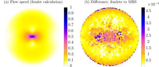
Figure 27: (a) The speed of the flow arising from a regularized force of the form (16), with $\epsilon=0.1$, situated at the origin in a no-slip circular cavity of radius $10$ as calculated by the method of femlets and (b) the absolute difference between the flow speed as calculated by the method of femlets and the method of regularized stokeslets.

We also wish to check that as the regularization of femlets is decreased, the femlet solution converges to that of an equivalent moving boundary. For the two-dimensional treadmilling squirmer of radius $r=L/2$ with slip velocity $u_{\theta}=A\sin\theta$ on $r=L/2$, in infinite fluid, the swimming velocity is given by $U=A/2$ ⁵². Whilst the finite element method is only applicable for finite domains, by taking a large enough open channel we may closely approximate a free swimmer in an infinite domain. For a channel of length $20L$ and height $10L$, the treadmilling squirmer is modeled by femlets with a Gaussian cut-off function, and the regularization parameters $\sigma_{x},\sigma_{y}$ varied.

The calculated swimming velocity in Newtonian fluid is given as a function of the regularizing parameters $\sigma_{x},\sigma_{y}$ in table 5. These results show that the difference associated with approximating a moving boundary by femlets decreases linearly with both $\sigma_{x}$ and $\sigma_{y}$.

Squirmer speed
# femlets	$\sigma_{x}$	$\sigma_{y}$	Velocity	Rel. error	$\mathrm{err}/\sigma_{y}$
$100$	$0.0222$	$0.0111$	$0.25897$	$0.0359$	$3.23$
$100$	$0.0222$	$0.00555$	$0.25462$	$0.0185$	$3.33$
$100$	$0.0222$	$0.00278$	$0.25246$	$0.00984$	$3.54$
$50$	$0.0444$	$0.0111$	$0.26067$	$0.0427$	$3.85$
$200$	$0.0111$	$0.00555$	$0.25421$	$0.0168$	$3.03$
$400$	$0.00555$	$0.00278$	$0.25192$	$0.00768$	$2.76$

Table 5: The velocity of the treadmilling squirmer as calculated with the method of femlets as a function of the regularization parameters $\sigma_{x},\sigma_{y}$, showing that the error associated in approximating a moving Dirichlet boundary by femlets decreases as approximately $\mathcal{O}(\sigma_{y})$.

The velocity field driven by the treadmilling squirmer in infinite fluid is given in cylindrical polar coordinates by ⁵²,

$$u_{r}(r,\theta)= \frac{1}{2}A\frac{(L/2)^{2}}{r^{2}}\cos\theta,$$ (19a)

$$u_{\theta}(r,\theta)= \frac{1}{2}A\frac{(L/2)^{2}}{r^{2}}\sin\theta.$$ (19b)

The relative error in the numerically calculated flow speed for $\sigma_{x}=0.0222,\sigma_{y}=0.00278$ is shown in figure 28. The error is approximately $\mathcal{O}(\sigma_{y})$, and is largest in the near field where the approximation of the boundary as an immersed regularized force driving the flow is most apparent.

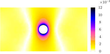
Figure 28: Relative error in the calculated speed of the flow induced by the treadmilling squirmer in Newtonian fluid, compared with the analytical solution of Blake ⁵² for an infinite fluid. The maximum relative error close to the squirmer is $1.2\%$, and is approximately $0.2\%$ throughout the majority of the domain.

References

- Hancock 1953 G. J. Hancock. The self-propulsion of microscopic organisms through liquids. Proc. Roy. Soc. Lond. A, 217:96–121, 1953.
- Johnson and Brokaw 1979 R. E. Johnson and C. J. Brokaw. Flagellar hydrodynamics. A comparison between Resistive-Force Theory and Slender-Body Theory. Biophys. J., 25(1):113–127, 1979.
- Cortez 2001 R. Cortez. The method of regularized Stokeslets. SIAM J. Sci. Comput., 23:1204–1225, 2001.
- Taylor 1967 G. I. Taylor. Low-Reynolds number flows. National Committee for Fluid Mechanics Films, available from http://web.mit.edu/hml/ncfmf.html, 1967.
- Purcell 1977 E. M. Purcell. Life at low Reynolds number. Amer. J. Phys., 45:3–11, 1977.
- Tam and Hosoi 2007 D. Tam and A. E. Hosoi. Optimal stroke patterns for Purcell’s three-link swimmer. Phys. Rev. Lett., 98(6):68105, 2007.
- Passov and Or 2012 E. Passov and Y. Or. Dynamics of Purcell’s three-link microswimmer with a passive elastic tail. Euro. Phys. J. E, 35(8):1–9, 2012.
- Najafi and Golestanian 2004 A. Najafi and R. Golestanian. Simple swimmer at low Reynolds number: three linked spheres. Phys. Rev. E, 69:062901, 2004.
- Polotzek and Friedrich 2012 K. Polotzek and B. M. Friedrich. A three-sphere swimmer for flagellar synchronization. arXiv preprint arXiv:1211.5981, 2012.
- Ledesma-Aguilar et al. 2012 R. Ledesma-Aguilar, H. Loewen, and J. M. Yeomans. A circle swimmer at low Reynolds number. Euro. Phys. J. E., 35(8):1–9, 2012.
- Ogrin et al. 2008 F. Y. Ogrin, P. G. Petrov, and C. P. Winlove. Ferromagnetic microswimmers. Phys. Rev. Lett., 100:218102–218106, 2008.
- Lai et al. 2009 S. K. Lai, Y. Y. Wang, D. Wirtz, and J. Hanes. Micro-and macrorheology of mucus. Adv. Drug Del. Rev., 61(2):86–100, 2009.
- Hall-Stoodley et al. 2004 L. Hall-Stoodley, J. W. Costerton, and P. Stoodley. Bacterial biofilms: from the natural environment to infectious diseases. Nat. Rev. Microbiol., 2(2):95–108, 2004.
- Verstraeten et al. 2008 N. Verstraeten, K. Braeken, B. Debkumari, M. Fauvart, J. Fransaer, J. Vermant, and J. Michiels. Living on a surface: swarming and biofilm formation. Trends Microbiol., 16(10):496–506, 2008.
- Fulford et al. 1998 G. R. Fulford, D. F. Katz, and R. L. Powell. Swimming of spermatozoa in a linear viscoelastic fluid. Biorheol., 35:295–310, 1998.
- Normand and Lauga 2008 T. Normand and E. Lauga. Flapping motion and force generation in a viscoelastic fluid. Phys. Rev. E, 78(6):061907, 2008.
- Lauga 2009 E. Lauga. Life at high Deborah number. Europhys. Lett., 86:64001, 2009.
- Elfring et al. 2010 G. J. Elfring, O. S. Pak, and E. Lauga. Two-dimensional flagellar synchronization in viscoelastic fluids. J. Fluid Mech., 646:505, 2010.
- Shen and Arratia 2011 X. N. Shen and P. E. Arratia. Undulatory swimming in viscoelastic fluids. Phys. Rev. Lett., 106(20):208101, 2011.
- Lauga 2007 E. Lauga. Propulsion in a viscoelastic fluid. Phys. Fluids, 19:083104–083117, 2007.
- Fu et al. 2009 H. C. Fu, C. W. Wolgemuth, and T. R. Powers. Swimming speeds of filaments in nonlinearly viscoelastic fluids. Phys. Fluids, 21:033102–033112, 2009.
- Zhu et al. 2012 L. Zhu, E. Lauga, and L. Brandt. Self-propulsion in viscoelastic fluids: Pushers vs. pullers. Phys. Fluids, 24(5):051902–051919, 2012.
- Teran et al. 2010 J. Teran, L. Fauci, and M. Shelley. Viscoelastic fluid response can increase the speed and efficiency of a free swimmer. Phys. Rev. Lett., 104:38101–38105, 2010.
- Lai et al. 2007 S. K. Lai, D. E. O’Hanlon, S. Harrold, S. T. Man, Y. Y. Wang, R. Cone, and J. Hanes. Rapid transport of large polymeric nanoparticles in fresh undiluted human mucus. Proc. Natl. Acad. Sci., 104(5):1482, 2007.
- Katz and Berger 1980 D. F Katz and S. A Berger. Flagellar propulsion of human sperm in cervical mucus. Biorheol., 17(1-2):169, 1980.
- Balmforth et al. 2010 N. J. Balmforth, D. Coombs, and S. Pachmann. Microelastohydrodynamics of swimming organisms near solid boundaries in complex fluids. Quart. J. Mech. App. Math., 63(3):267–294, 2010.
- Shen et al. 2012 X. Shen, D. Gagnon, and P. Arratia. Undulatory swimming in shear-thinning fluids. Bull. Amer. Phys. Soc., 57, 2012.