Comment on “Ratchet universality in the presence of thermal noise”

Abstract

A recent paper [Phys. Rev. E 87, 062114 (2013)] presents numerical simulations on a system exhibiting directed ratchet transport of a driven overdamped Brownian particle subjected to a spatially periodic, symmetric potential. The authors claim that their simulations prove the existence of a universal waveform of the external force which optimally enhances directed transport, hence confirming the validity of a previous conjecture put forward by one of them in the limit of vanishing noise intensity. With minor corrections due to noise, the conjecture holds even in the presence of noise, according to the authors. On the basis of their results the authors claim that all previous theories, which predict a different optimal force waveform, are incorrect. In this comment we provide sufficient numerical evidence showing that there is no such universal force waveform and that the evidence obtained by the authors otherwise is due to a fortunate choice of the parameters. Our simulations also suggest that previous theories correctly predict the shape of the optimal waveform within their validity regime, namely when the forcing is weak. On the contrary, the aforementioned conjecture is shown to be wrong.

The authors of Ref. Martínez and Chacón (2013a) (see also the erratum Martínez and Chacón (2013b)) simulate the equation

$$\begin{split}&\dot{x}+\sin x=\sqrt{\sigma}\xi(t)+\gamma F_{\text{bihar}}(t),\\ &F_{\text{bihar}}(t)=\eta\sin(\omega t)+2(1-\eta)\sin(2\omega t+\phi),\end{split}$$ (1)

where $\gamma$ is the global amplitude of the force; $0\leqslant\eta\leqslant 1$ and $\phi$ account for the relative amplitude and initial phase difference of the two harmonics, respectively; $\xi(t)$ is a Gaussian white noise with zero mean and $\langle\xi(t)\xi(t+s)\rangle=\delta(s)$; and $\sigma$ is proportional to the temperature of the system. This system exhibits ratchet transport if the external force breaks both, a time-shift symmetry, namely if $F_{\text{bihar}}(t)\neq-F_{\text{bihar}}(t+T/2)$ ($T$ being the period of $F_{bihar}$), and time-reversal, i.e., $F_{\text{bihar}}(t)\neq-F_{\text{bihar}}(-t)$. This happens for all $0<\eta<1$ and all $\phi\neq 0,\pi$. If initially the particle starts at $x(t_{0})=x_{0}$, the ratchet current can be obtained as

$$v=\lim_{t\to\infty}\frac{\langle x(t)\rangle-x_{0}}{t-t_{0}},$$ (2)

where $\langle\cdot\rangle$ represents an ensemble average over all trajectories satisfying the same initial condition.

Obviously the ratchet current $v$ will be a function of the parameters of the system, in particular of those that define the external force. Since for $\eta=0$, $1$ or $\phi=0$, $\pi$ the force neither breaks the time-shift symmetry nor the time-reversal symmetry (hence $v=0$), it is easily foreseen that for a certain combination of the parameters of the force $v$ must be maximal (in absolute value).

Based on a conjecture proposed by one of the authors Chacón (2010), $v$ should be optimal when the force maximally breaks the symmetries. For $\sigma=0$ this happens for $\eta=4/5$ irrespective of the value of $\gamma$ and of $\phi$ (as long as $\phi\neq 0,\pi$) Martínez and Chacón (2013a). An argument based on an affine transformation of the force leads the authors to conclude that this optimal shape of the force will hold even for $\sigma>0$ —albeit some deviations are to be expected.

This result is universal in the sense that is independent of $\gamma$ and $\phi$. Figure 1(a) of Martínez and Chacón (2013b) confirms that this is an accurate prediction even for the high intensities of the noise they use in their simulations ($\sigma=2$, $3$, $4$). The other parameters are set to $\omega=0.08\pi$, $\phi=\pi/2$, and $\gamma=2$ throughout their paper.

They go on to claim that, since all previous theories Hänggi and Marchesoni (2009); Flach et al. (2000); Denisov et al. (2002); Wonneberger and Breymayer (1981); Marchesoni (1986); Quintero et al. (2010) predict a form of the ratchet current given by Martínez and Chacón (2013b)

$$v\propto\gamma^{3}\eta^{2}(1-\eta),$$ (3)

they all predict that $v$ is optimal for $\eta=2/3$, a value certainly far away from the simulation results.

Accordingly the two main conclusions of this work are: (i) the conjecture of a universal force waveform which optimizes the current is confirmed even in the presence of strong noise —albeit with some deviations—, and (ii) all previous theories must be incorrect because they incorrectly predict this form.

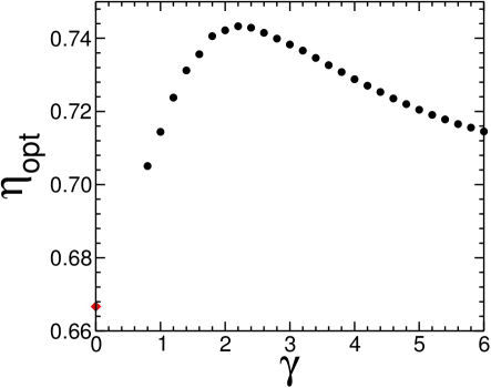
Figure 1: (Color online) Values of the parameter $\eta$ defining the relative amplitudes of the two harmonics of the external force $F_{\text{bihar}}(t)$ [c.f. Eq. (1)], for which the ratchet velocity $v$ reaches its maximum absolute value, plotted as a function of the global amplitude of the external force $\gamma$ (full black dots). The remaining parameters are chosen as in Fig. 1 of Martínez and Chacón (2013a) (actually of the erratum Martínez and Chacón (2013b)): $\omega=0.08\pi$, $\sigma=2$, $\phi=\pi/2$. The red diamond at $(0,2/3)$ represents the theoretical prediction of previous theories Hänggi and Marchesoni (2009); Flach et al. (2000); Denisov et al. (2002); Wonneberger and Breymayer (1981); Marchesoni (1986); Quintero et al. (2010), which should hold in the limit $\gamma\to 0$.

We have carried out extensive simulations of the same system (1) and with the same parameter as the authors of Martínez and Chacón (2013a, b), but instead of limiting ourselves to the single value of the global amplitude $\gamma=2$ used in their simulations we have covered a wider range of values, from $\gamma=6$ down to $\gamma=0.8$. Below this value simulations are prohibitively long because the high values of the noise intensity demand a very large number of realizations to achieve reliable results. The outcome of these simulations is summarized in Fig. 1, which represents the value of $\eta$ (henceforth $\eta_{\text{opt}}$) which optimizes $v$ as a function of the global amplitude of the external force $\gamma$.

There are three main conclusions that we can extract from this figure. First of all, there is no such thing as an optimal force waveform. The values of $\eta_{\text{opt}}$ range from near $0.69$ up to near $0.75$. The predicted universal value $\eta_{\text{opt}}=4/5$ is reached at no value of $\gamma$, and the closest it gets to it is at $\gamma\approx 2$ —precisely the value used in the simulations of Ref. Martínez and Chacón (2013a, b). We need to make clear at this point that setting $\gamma=2$ in our simulations our results reproduce accurately the plots of Fig. 1(a) of this work. This leads us to our second conclusion, namely that the authors of this work have been misled by their specific choice of the simulation parameters. Finally, although we cannot decrease $\gamma$ below $0.8$ without introducing too much uncertainty, the figure clearly illustrates that the trend of the value of $\eta$ which optimizes $v$ is toward the value $2/3$ which all theories predict in their range of validity, i.e., in the limit of weak external forces.

On the basis of this evidence we conclude that the conjecture put forward in Chacón (2010) is wrong, no matter how appealing it may sound. The reasoning leading from maximum symmetry breaking of the external force to a maximum response of the system is of a “linear response” style, and does not hold for the kind of nonlinear behavior that ratchet current generation represents.

For the sake of reproducibility we provide the details of the numerical procedure we have followed to obtain Fig. 1. Simulations of the stochastic differential equation (1) have been performed using the 2nd order weak predictor-corrector method Kloeden and Platen (1995) with time-step $\Delta t=0.01$, initial condition $x(0)=0$, and a final integration time $t_{f}=200\pi/\omega$. The ratchet velocity $v$ has been computed using formula (2) averaging over 5000 realizations of the noise. For each $\gamma$ in Fig. 1 we have obtained an entire curve $v(\eta)$ for $100$ values of $\eta$ in the interval $[0,1]$.

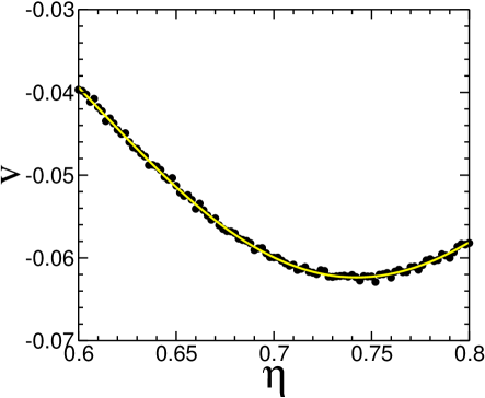
Figure 2: (Color online) Value of the ratchet current $v$ as a function of the parameter $\eta$ defining the relative amplitudes of the two harmonics of the external force $F_{\text{bihar}}(t)$ [c.f. Eq. (1)]. Parameters: $\gamma=2$, $\omega=0.08\pi$, $\sigma=2$, $\phi=\pi/2$. Bullets are the results from simulations averaged over 5000 realizations of the noise. The yellow curve is a fourth order polynomial fit to these results ($v=-3.7188+22.068\eta-48.018\eta^{2}+44.984\eta^{3}-15.366\eta^{4}$; correlation coefficient $r=0.99$). This fit is used to determine $\eta_{\text{opt}}$. Notice that the minimum of the fit (at $\eta=0.742$) does not coincide with the value of $\eta$ for which the largest absolute value of $v$ occurs because of the fluctuations in the ratchet current.

Despite the average over such a large number of realizations, the resulting curves are still quite noisy —too much to reliably determine the value $\eta_{\text{opt}}$. For this reason we have recalculated the curves $v(\eta)$ for another $100$ values of $\eta$ in a narrower interval that clearly contains $\eta_{\text{opt}}$, and have fitted a fourth degree polynomial to the results (see Fig. 2 for an example). The value of $\eta_{\text{opt}}$ is obtained by optimizing this polynomial. This is how the points of Fig. 1 have been obtained.

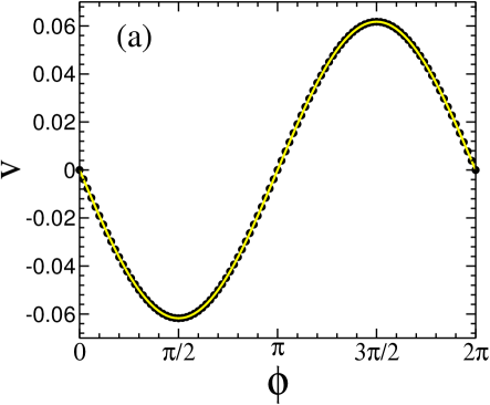
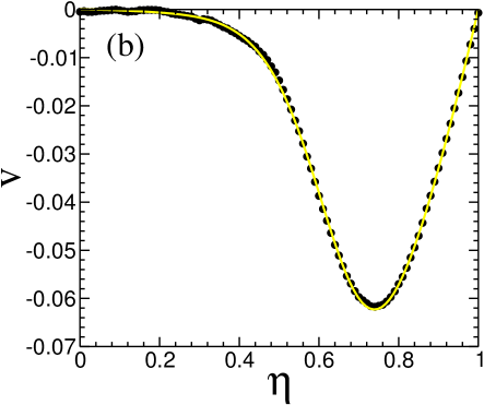
Figure 3: (Color online) (a) $v$ as a function of $\phi$ for $\eta=2/3$, (b) ratchet current $v$ as a function of $\eta$, for $\phi=\pi/2$. Bullets are the numerical simulations of Eq. (1) with parameters $\omega=0.08\pi$, $\sigma=2$, and $\gamma=2$. The yellow solid line in (a) is a fit to a sinusoidal function ($v=-0.062\sin\phi$). The yellow solid line in (b) is a fit to $-\eta^{2}(1-\eta)A(\eta)$, where $A(\eta)$ is the $(2,2)$-Padé approximant $A(\eta)=(0.025-0.113\eta+0.212\eta^{2})(1-2.662\eta+2.011\eta^{2})^{-1}$.

As for the second conclusion of Ref. Martínez and Chacón (2013a), aside from the evidence provided by Fig. 1 that the numerical results are consistent with the $\eta_{\text{opt}}=2/3$ prediction of the theories in the limit of weak external forces, we can actually go further and show that a recent extension of the theory developed in Ref. Quintero et al. (2010), valid for arbitrarily large forces Cuesta et al. (2013), fits perfectly with the results presented in Martínez and Chacón (2013a, b). For the case of harmonic mixing represented by Eq. (1), the theory predicts that $v$ is given by the harmonic expansion

$$v=\sum_{n=0}^{\infty}A_{n}(\gamma,\eta)\gamma^{6n+3}\eta^{4n+2}(1-\eta)^{2n+1}\sin[(2n+1)\phi],$$ (4)

where the coefficients $A_{n}(\gamma,\eta)$ are functions of the squares of the amplitudes of the forcing harmonics, i.e., of $\gamma^{2}\eta^{2}$ and $\gamma^{2}(1-\eta)^{2}$. This implies that, if the current is well described by one sinusoidal function, then

$$v=A_{0}(\gamma,\eta)\gamma^{3}\eta^{2}(1-\eta)\sin\phi+O(\gamma^{9}),$$ (5)

and $A_{0}(\gamma,\eta)$ should be well described by a bivariate quadratic polynomial —or any other approximant of an equivalent order— in $\gamma^{2}\eta^{2}$ and $\gamma^{2}(1-\eta)^{2}$.

Figure 3 (top) shows a fit of a sinusoidal function to the simulation data for $v$ as a function of $\phi$ obtained from Eq. (1) for $\eta=2/3$ and the other parameters as in Fig. 1 of Martínez and Chacón (2013b). It clearly shows that retaining only the first harmonic in (4) is enough to accurately reproduce the data. Thus $v$ should conform to (5). Accordingly, we set $\phi=\pi/2$ and fit the simulation results of $v$ vs. $\eta$ to a function of the form $-\eta^{2}(1-\eta)A(\eta)$, where we take for $A(\eta)$ a $(2,2)$-Padé approximant . The result is plotted in Fig. 3 (bottom) to show that this fit is a very accurate description of $v(\eta)$ —and therefore correctly predicts the deviation of $\eta_{\text{opt}}$ from its weak force approximation $\eta_{\text{opt}}=2/3$.

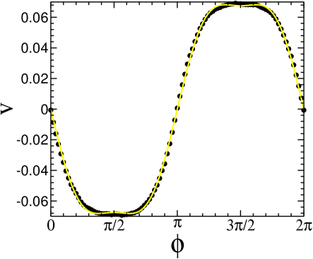
Figure 4: (Color online) $v$ as a function of $\phi$ for $\eta=2/3$, $\gamma=6$, $\omega=0.08\pi$, and $\sigma=2$. Bullets are the numerical simulations of Eq. (1). The yellow solid line in the top panel is a fit to the two first harmonics of Eq. (4) ($v=-0.079\sin\phi-0.011\sin 3\phi$).

Finally we would like to point out that the idea of an optimal shape of the external force is very difficult to reconcile with the current shape given by Eq. (4), because as soon as the amplitude of the force $\gamma$ becomes sufficiently large, new harmonics will start modulating the shape of the current (Fig. 4 clearly illustrates this effect). In this regime, only a very specific dependence of the coefficients $A_{n}$ with $\gamma$ —which does not occur in the case of Eq. (1)— would yield the universality claimed in Chacón (2010); Martínez and Chacón (2013a, b).