Hierarchical equations of motion for impurity solver in dynamical mean-field theory

Abstract

A nonperturbative quantum impurity solver is proposed based on a formally exact hierarchical equations of motion (HEOM) formalism for open quantum systems. It leads to quantitatively accurate evaluation of physical properties of strongly correlated electronic systems, in the framework of dynamical mean-field theory (DMFT). The HEOM method is also numerically convenient to achieve the same level of accuracy as that using the state-of-the-art numerical renormalization group impurity solver at finite temperatures. The practicality of the novel HEOM+DMFT method is demonstrated by its applications to the Hubbard models with Bethe and hypercubic lattice structures. We investigate the metal-insulator transition phenomena, and address the effects of temperature on the properties of strongly correlated lattice systems.

I Introduction

Strongly correlated electronic systems (SCS) generally refer to materials with d- or f-electrons. These localized electrons strongly interact with each other and with the surrounding itinerant electrons, leading to various intriguing many-body phenomena, such as Kondo phenomena, metal-insulator transition in transition metal oxides, and heavy fermion in rare-earth compounds. SCS quickly becomes an active research area in condensed matter physics.Ful95

Exact treatment of SCS for classic band theory and model methods is difficult because of the nonperturbative many-body nature and the complexity of SCS materials. Since the proposal of investigating SCS in the limit of infinite dimension in 1989,Met89324 the dynamical mean-field theory (DMFT)Jar92168 ; Geo926479 ; Geo9613 has been rapidly developed and applied, leading to a dramatic progress in understanding the properties of SCS. In this limit, the self-energy is local, so that the spatial fluctuations in strongly correlated systems can be neglected while only the on-site Coulomb interaction is taken into consideration. As a result, the many-body lattice problem is mapped to an effective impurity problem, in which the correlated electrons on the impurity site interacts with a frequency dependent mean field. This mean field is then updated in a self-consistent way via the solution of the impurity model in order to obtain the self-energy of the lattice Green’s function.

The DMFT method was firstly used with Hubbard model, and revealed the three-peak spectral function induced by the strong electron-electron correlation.Jar92168 ; Geo926479 These three peaks are comprised of one central quasi-particle peak around the Fermi energy and two single-particle Hubbard peaks. In some transition metal oxides, the central quasi-particle peak gradually transfers its weight to the Hubbard peaks with increasing Coulomb interaction,Zha931666 finally leading to metal-insulator transition, which is usually referred to as Mott transition.Geb97 It is one of the most fascinating phenomena of SCS that has been observed in various transition metal oxides,Ima981039 and extensively investigated by DMFT methods.Geo937167 ; Roz9410181 ; Roz993498 ; Bul99136 ; Bul01045103 ; Dai05045111 ; Ono03035119 ; Flo02165111 In recent years, the DMFT methods have been extended to the investigations of some complicated SCS with multi orbital, nonlocal Coulomb and exchange interaction, or taking into account spatial correlations.Si963391 ; Chi003678 ; Kot2001 ; Drc0561 ; Kus06054713 ; Tos07045118 Especially, the combination of DMFT method with density functional theory makes it possible to simulate complicated real compounds with strong electron correlations.Ani977359 ; Kot06865 The DMFT method has already been a powerful tool for the investigation of strongly correlated physics.

The accuracy and efficiency of DMFT calculation is determined by the key component, the impurity solver, that solves the effective impurity problem. A vast amount of theoretical efforts have been devoted to achieving this goal. The perturbative methods such as the iterated perturbation theoryKaj9616214 and non-crossing approximationBic87845 sum the perturbative series of interaction diagrams to different orders, resulting in different levels of accuracy. Extensions of these methods to away from half filling (iterated perturbation theory) or to very low temperature regime (non-crossing approximation) are technically complicated, which largely limit the applications of these methods. The currently used nonperturbative methods include the exact diagonalization approach,Dag94763 ; Caf941545 ; Si942761 quantum Monte Carlo approach,Hir862521 ; Gul11349 and numerical renormalization group (NRG) method.Wil75773 ; Bul08395 ; Hof001508 ; Wei07076402 ; Pet06245114

Although the existing methods have been successfully used in characterizing the fundamental characteristics of SCS, they have their own limitations.And6141 ; Hub63238 ; Lee8699 Both the exact diagonalization approach and the configuration interaction methods diagonalize the Hamiltonian in a finite dimensional Hilbert space. In DMFT applications, the continuous bath degrees of freedom are discretized and a small number of bath sites (orbitals) are chosen to represent the full bath. Consequently, the local density of states is composed of discrete peaks which are then broadened artificially. The energy resolution in the spectrum depends on the number of bath sites. Therefore, although the quasiparticle weight $Z$ can be extracted from the Matsubara Green’s function, it is difficult to obtain the real frequency quantities,Ani2010 including the low energy Kondo peak and the high energy Hubbard peaks; see for instance, Fig. S11 in the Supplemental Material of Ref. Li12266403, . The computational cost of some quantum Monte Carlo (QMC) approaches, including the Hirsch-Fye algorithm and the continuous time QMC, increases dramatically as the temperature decreases. Moreover, numerical methods such as the maximum entropy method are often required to extract real frequency spectral function from the imaginary time domain via some analytic continuation operation. This may introduce additional errors.Jar96133 In recent years the NRG method has achieved significant progress, thanks to the improvement of its algorithm and advancement of computer hardware. However, some of its basic features have remained unchanged: It utilizes logarithmic discretization and truncation of energy spectrum during iterative diagonalization. Therefore, quantities produced by the NRG method are less accurate at high energy or high temperatures than at low energy or low temperatures.Bul08395 Therefore, an accurate and efficient DMFT impurity solver for the investigation of the strong correlation effects at finite temperatures is highly desirable.

In this work we propose to use a hierarchical equations of motion (HEOM) approachJin08234703 as the impurity solver of DMFT. The HEOM method treats quantum impurity systems from the perspective of open dissipative dynamics. As will be discussed in Sec. II.1, in principle the HEOM formalism is formally exact, as long as the bath environment satisfies Gaussian statistics, which is true for noninteracting electron reservoirs. The HEOM theory can be established based on the Feynman–Vernon path-integral formalism,Jin08234703 ; Fey63118 ; Kle09 ; Xu05041103 ; Xu07031107 in which all the system-bath correlations are taken into consideration.

In practice, the HEOM method is implemented without invoking any approximation or any tricky controlling parameter. The numerical results are quantitatively accurate for a wide range of impurity systems, as long as they converge with respect to the increasing truncation level $L$.

Usually, the HEOM results converge uniformly and rapidly with the increasing $L$. A higher $L$ is needed to achieve numerical convergence at a lower temperature. Consequently, the computational cost increases substantially as the temperature lowers. Currently for a symmetric single impurity Anderson model, the HEOM approach reaches quantitatively accuracy for temperature $T\geqslant 0.1\,T_{\rm K}$ (Kondo temperature) with the computational resources at our disposal.Li12266403 In particular, the HEOM approach remains accurate at high temperature and large frequency (energy) range. For all the results presented in this work, $L$ is chosen to be sufficiently large so that numerical convergence is always guaranteed.

The HEOM approach is applicable to a general quantum impurity system. It is capable of treating strongly correlated impurities with more than one orbitals. The applicability of HEOM approach to various equilibrium and nonequilibrium properties of quantum dot systems has been demonstrated.Zhe08184112 ; Wan13035129 These include the studies on dynamical Coulomb blockadeZhe08093016 and dynamical Kondo transitions in quantum dots.Zhe09164708 ; Zhe13086601 Previous studies have shown that the HEOM approach is capable of achieving the accuracy of the latest high-level NRG approach, as demonstrated by the impurity spectral functionsLi12266403 and the local magnetic susceptibilityWan13035129 of Anderson impurity model systems at finite temperatures. All these successful applications suggest that the HEOM approach is very suitable to be used as an impurity solver in the framework of DMFT method.

The remainder of this paper is organized as follows. The HEOM based impurity solver is introduced in Sec. II, together with its main features and current limitations. In Sec. III, the results for the Mott transition from DMFT using HEOM impurity solver are systematically compared with previous NRG results to show its accuracy and efficiency. Concluding remarks are finally given in Sec. IV.

II Hierarchical equations of motion based DMFT impurity solver

II.1 A formally exact HEOM formalism for quantum impurity systems

The HEOM approach is based on quantum dissipation theory, which can be used to characterize the quantum impurity systems as open systems embedded in surrounding environments composed of itinerant electron reservoirs. The derivation of the HEOM formalism has been detailed in Refs. Jin08234703, , Zhe09164708, , and Zhe121129, . Here, we introduce some of its basic features.

The Hamiltonian of the quantum impurity system can be expressed as

$$H_{{\rm total}}=H_{\text{\scriptsize sys}}+H_{\text{\scriptsize res}}+H_{\text{\scriptsize sys-res}},$$ (1)

where $H_{\text{\scriptsize sys}}$ represents the quantum impurity systems containing strong correlation interactions, $H_{\text{\scriptsize res}}=\sum_{k}\epsilon_{k}\hat{d}^{\dagger}_{k}\hat{d}_{k}$ is the noninteracting electron reservoirs, and $H_{\text{\scriptsize sys-res}}=\sum_{\mu k}(t_{\mu k}\,\hat{a}^{\dagger}_{\mu}\hat{d}_{k}+{\rm H.c.})$ accounts for the impurity-reservoir couplings. In these terms, $\hat{a}_{\mu}^{\dagger}$ and $\hat{a}_{\mu}$ are the creation and annihilation operators for the impurity state $|\mu\rangle$; $\hat{d}_{k}^{\dagger}$ and $\hat{d}_{k}$ are those for the reservoir state $|k\rangle$ of energy $\epsilon_{k}$. The hybridization functions of the electron reservoir are defined as $\Delta_{\mu\nu}(\omega)\equiv\pi\sum_{k}t_{\mu k}t^{\ast}_{\nu k}\,\delta(\omega-\epsilon_{k})$.

In the quantum dissipation theory, the quantity of primary interest is the reduced density matrix of the impurity system, $\rho(t)\equiv{\rm tr}_{\text{\scriptsize res}}\,\rho_{{\rm total}}(t)$. Here, $\rho_{{\rm total}}(t)$ is the density matrix of the total system (impurity plus electron reservoir); and ${\rm tr}_{\text{\scriptsize res}}$ denotes the trace over all reservoir’s degrees of freedom. The dynamics of the reduced density matrix can be characterized by a Liouville-space quantum propagator $\mathcal{U}(t,t_{0})$ as follows,

$$\rho(t)=\mathcal{U}(t,t_{0})\rho(t_{0}).$$ (2)

The specific form of $\mathcal{U}(t,t_{0})$ can be expressed using the Feynmann–Vernon path integral representation ofFey63118

$$\mathcal{U}(t,t_{0})=\int_{t_{0}}^{t}\mathcal{D}\psi\int_{t_{0}}^{t}\mathcal{D}\psi^{\prime}\,e^{iS[\psi]}\,\mathcal{F}[\psi,\psi^{\prime}]\,e^{-iS[\psi^{\prime}]}.$$ (3)

Here, $S[\psi]$ is the classical action functional associated with $H_{\text{\scriptsize sys}}$. For the convenience of evaluating expectation values, usually an initial factorization ansatz is adopted for the total system at $t_{0}=-\infty$:

$$\rho_{{\rm total}}(t_{0})=\rho(t_{0})\otimes\rho_{\text{\scriptsize res}}^{\rm eq},$$ (4)

with $\rho_{\text{\scriptsize res}}^{\rm eq}$ being the equilibrium reduced density matrix of reservoir environment. We emphasize that the uncorrelated total system at $t_{0}=-\infty$ is chosen only as a reference for the construction of $\mathcal{U}(t,t_{0})$. For the calculation of any physical quantity or process, we first solve for the fully correlated stationary state $\rho(t_{0}^{\prime})$ at a finite time $t_{0}^{\prime}$, and then use $\rho(t_{0}^{\prime})$ as the initial condition for subsequent dynamics of the impurity system.

It is $\mathcal{F}[\psi,\psi^{\prime}]$ that accounts for the influence of the dissipative reservoir environment to the properties of the impurity, and it is thus termed as the influence functional, which has the following form:Jin08234703

$$\mathcal{F}[\psi,\psi^{\prime}] \equiv\exp\left\{-\int_{t_{0}}^{t}d\tau\,\mathcal{R}[\tau;\psi,\psi^{\prime}]\right\},$$ (5)

$$\mathcal{R}[t;\psi,\psi^{\prime}] =\sum_{\sigma\mu}a_{\mu}^{\bar{\sigma}}(\psi(t))\left[B^{\sigma}_{\mu}(t;\psi)-B^{\prime\sigma}_{\mu}(t;\psi^{\prime})\right]-$$

$$\qquad\left[B^{\sigma}_{\mu}(t;\psi)-B^{\prime\sigma}_{\mu}(t;\psi^{\prime})\right]a_{\mu}^{\bar{\sigma}}(\psi^{\prime}(t)),$$ (6)

$$B^{\sigma}_{\mu}(t;\psi) \equiv\sum_{\nu}\int^{t}_{t_{0}}d\tau\,C^{\sigma}_{\mu\nu}(t,\tau)\,a^{\sigma}_{\nu}(\psi(\tau)),$$ (7)

$$B^{\prime\sigma}_{\mu}(t;\psi^{\prime}) \equiv\sum_{\nu}\int^{t}_{t_{0}}d\tau\,C^{\bar{\sigma}\ast}_{\mu\nu}(t,\tau)\,a^{\sigma}_{\nu}(\psi^{\prime}(\tau)),$$ (8)

where $\sigma=+/-$ and $\bar{\sigma}=-\sigma$. It should be emphasized that the above Eq. (6) is an exact formula, as long as the reservoir environment satisfies Gaussian statistics, which is true for reservoirs consisting of noninteracting electrons.Jin08234703

Although $\mathcal{F}[\psi,\psi^{\prime}]$ has a rather complicated form, it is apparent that the impurity-reservoir coupling $H_{\text{\scriptsize sys-res}}$ enters (exclusively) through the reservoir correlation function (or memory kernel) $C^{\sigma}_{\mu\nu}(t,\tau)$. Therefore, with the exact $C^{\sigma}_{\mu\nu}(t,\tau)$ at hand, we can obtain the exact Liouville propagator $\mathcal{U}(t,t_{0})$ and hence the exact $\rho(t)$ via the path integral of Eq. (3).

For a noninteracting reservoir, the correlation function $C^{\sigma}_{\mu\nu}(t,\tau)$ is fully determined by the reservoir hybridization function $\Delta_{\mu\nu}(\omega)$ via the following fluctuation-dissipation theorem:

$$C^{\sigma}_{\mu\nu}(t,\tau) =\exp\left\{\bar{\sigma}i\int_{\tau}^{t}dt^{\prime}\,V(t^{\prime})\right\}\,\tilde{C}^{\sigma}_{\mu\nu}(t-\tau),$$

$$\tilde{C}^{\sigma}_{\mu\nu}(t) =\int_{-\infty}^{\infty}d\omega\,e^{\sigma i\omega t}f^{\sigma}_{\beta}(\omega)\Delta^{\sigma}_{\mu\nu}(\omega).$$ (9)

Here, $V(t)$ is the time-dependent bias voltage applied to the reservoir, $\Delta^{+}_{\nu\mu}(\omega)=\Delta^{-}_{\mu\nu}(\omega)=\Delta_{\mu\nu}(\omega)$. $f^{\sigma}_{\beta}(\omega)=1/[1+e^{\sigma\beta(\omega-\epsilon_{f})}]$ is the Fermi function for electron ($\sigma=+$) or hole ($\sigma=-$), $\beta=1/k_{B}T$, and $\epsilon_{f}$ is the equilibrium chemical potential of reservoir. In fact, $\tilde{C}^{\sigma}_{\mu\nu}(t)$ are exactly equivalent to the “embedding” self energies: $\tilde{C}^{+}_{\mu\nu}(t)=i[\Sigma^{<}_{\mu\nu}(t)]^{\ast}$ and $\tilde{C}^{-}_{\mu\nu}(t)=i\Sigma^{>}_{\mu\nu}(t)$.Jin08234703

Clearly, $\mathcal{U}(t,t_{0})$ can be obtained via the formally exact path integral formalism by combining Eqs. (3)–(9). The only requirement is the reservoir should consist of noninteracting electrons, and hence the reservoir environment satisfies Gaussian statistics. With the resulted $\rho(t)$, the expectation value of any system operator $\hat{A}$ can then be calculated as $\langle\hat{A}\rangle={\rm tr}[\hat{A}\rho(t)]$.

In practice, the path integral formalism will lead to an integro-differential quantum master equation for $\rho(t)$, and hence very difficult to solve. To circumvent this problem, an HEOM formalism is instead proposed. In the HEOM formalism, the integro-differential equation is replaced by a hierarchical set of linear differential equations. As a consequence, the numerical calculations become much more convenient.

The central step towards the establishment of HEOM is the decomposition of reservoir memory kernel $\tilde{C}^{\sigma}_{\mu\nu}(t)$ into exponential functions, i.e.,

$$\tilde{C}^{\sigma}_{\mu\nu}(t)=\sum_{m=1}^{M}\eta^{\sigma}_{\mu\nu m}\,e^{-\gamma^{\sigma}_{\mu\nu m}t},$$ (10)

where $1/{\rm Re}[\gamma^{\sigma}_{\mu\nu m}]$ is the characteristic memory time of $m$th dissipation mode. A number of memory decomposition schemes have been developed, including the conventional Matsubara decomposition scheme,Jin08234703 a hybrid spectrum decomposition and frequency dispersion scheme,Zhe09164708 the partial fraction decomposition scheme,Cro09073102 and the Padé spectrum decomposition scheme.Oza07035123 ; Hu10101106 ; Hu11244106

Most of the existing memory decomposition schemes are based on a contour integral algorithm for Eq. (9) with the use of a residual theorem,Zhe09164708 and each exponential term in Eq. (10) corresponds to a pole of complex function $f^{\sigma}_{\beta}(z)$ or $\Delta_{\mu\nu}(z)$ in Eq. (9), via the following expansions:

$$f^{\sigma}_{\beta}(z) \simeq\frac{1}{2}-\sigma\frac{1}{\beta}\sum_{p=1}^{P}\left(\frac{1}{z+z_{p}}-\frac{1}{z-z_{p}}\right),$$ (11)

$$\Delta_{\mu\nu}(z) \approx\sum_{i=1}^{N}\frac{\eta_{\mu\nu,i}}{(z-\Omega_{\mu\nu,i})^{2}+(W_{\mu\nu,i})^{2}}.$$ (12)

Therefore, the total number of memory components is $M=P+N$, with $P$ and $N$ being the number of poles for $f^{\sigma}_{\beta}(z)$ and $\Delta^{\sigma}_{\mu\nu}(z)$ in the upper or lower $z$-plane, respectively.

Note that Eq. (11) is a formal expansion of the Fermi function, and the choice of $\{z_{p}\}$ is not unique. At any finite temperature, $P$ can always be chosen so that the right-hand side of Eq. (11) and their contributions to $\tilde{C}^{\sigma}_{\mu\mu}(t)$ converge to a preset precision. To the best of our knowledge, the Padé expansion of $f^{\sigma}_{\beta}(z)$ requires a smallest $P$, and thus is by far the most efficient scheme for Eq. (11).Hu11244106 In contrast, Eq. (12) is realized by a least square fit of $\Delta_{\mu\nu}(\omega)$ to a linear combination of Lorentzian functions, with $\{\eta_{\mu\nu,i},\Omega_{\mu\nu,i},W_{\mu\nu,i}\}$ being the fitted parameters. The accuracy of the resulted memory decomposition is determined by the quality of the least square fit. For a continuous $\Delta_{\mu\nu}(\omega)$ the fitting of Eq. (12) is usually satisfactory; see for instance Fig. 2 in Sec. II.4. Therefore, the combined Padé-Lorentzian schemeWan13205126 achieves an accurate and efficient exponential decomposition of $\tilde{C}^{\sigma}_{\mu\nu}(t)$ via Eq. (10).

With the exponential decomposition of reservoir memory, the HEOM can be cast into a compact form asJin08234703

$$\dot{\rho}^{(n)}_{j_{1}\cdots j_{n}}= -\Big{(}i{\cal L}+\sum_{r=1}^{n}\gamma_{j_{r}}\Big{)}\rho^{(n)}_{j_{1}\cdots j_{n}}-i\sum_{j}\!{\cal A}_{\bar{j}}\,\rho^{(n+1)}_{j_{1}\cdots j_{n}j}$$

$$-i\sum_{r=1}^{n}(-)^{n-r}\,{\cal C}_{j_{r}}\,\rho^{(n-1)}_{j_{1}\cdots j_{r-1}j_{r+1}\cdots j_{n}}.$$ (13)

Here, $\rho^{(0)}(t)=\rho(t)\equiv{\rm tr}_{\text{\scriptsize res}}\,\rho_{{\rm total}}(t)$ is the reduced density matrix, and $\{\rho^{(n)}_{j_{1}\cdots j_{n}}(t);n=1,\cdots,L\}$ are the auxiliary density matrices, with $L$ being the truncation level. The multi-component index $j\equiv(\sigma\mu\nu m)$. The Grassmann superoperators ${\cal A}_{\bar{j}}\equiv{\cal A}^{\bar{\sigma}}_{\mu}$ and ${\cal C}_{j}\equiv{\cal C}^{\sigma}_{\mu\nu m}$ are defined via their actions on a fermionic/bosonic operator $\hat{O}$ as ${\cal A}^{\bar{\sigma}}_{\mu}\hat{O}\equiv[\hat{a}^{\bar{\sigma}}_{\mu},\hat{O}]_{\mp}$ and ${\cal C}^{\sigma}_{\mu\nu m}\hat{O}\equiv\eta^{\sigma}_{\mu\nu m}\hat{a}^{\sigma}_{\nu}\hat{O}\pm(\eta^{\bar{\sigma}}_{\mu\nu m})^{\ast}\hat{O}\hat{a}^{\sigma}_{\nu}$, respectively, with $\bar{\sigma}$ denoting the opposite sign of $\sigma=+/-$. The electron correlation interaction is contained in the Liouvillian of impurities, $\mathcal{L}\,\cdot\equiv[H_{\text{\scriptsize sys}},\cdot\,]$.

Moreover, the subscript index set ($j_{1}\cdots j_{n}$) in an $n^{\rm th}$-level auxiliary density matrix $\rho^{(n)}_{j_{1}\cdots j_{n}}$ belongs to an ordered set of $n$ distinct $j$-indices. The number of distinct $j$-indices, $K$, is equal to not only the number of the first-level auxiliary density matrices in total, but also the maximum hierarchical level ($L_{\rm max}=K$). Therefore, the number of the $n^{\rm th}$-level auxiliary density matrices is $\frac{K!}{n!(K-n)!}$. Then, the total number of unknowns to solve ${\cal N}(K,L)$, which dominates the computational cost of the HEOM approach, is the summation over all the truncation level, $\sum_{n=0}^{L}\frac{K!}{n!(K-n)!}\leqslant 2^{K}$, as $L\leqslant K$. In this expression, $K$ can be evaluated by $K=2MN_{\mu}$, in which $M$ is determined by the resolution of the bath memory, and $N_{\mu}$ is the number of the system states (orbitals) that couple directly to electron reservoirs. This scheme provides an optimal basis to exploit the different characteristic time scales associated with system-reservoir dissipation processes. The hierarchy terminates automatically at $L=2$ for noninteracting $H_{\text{\scriptsize sys}}$;Jin08234703 while for $H_{\text{\scriptsize sys}}$ involving electron correlation interactions, the solution of Eq. (II.1) must go through systematic tests to confirm its convergence versus $L$. In practice, recent investigations on a general quantum impurity system have indicated that a relatively low $L$ ($\simeq 4$) is usually sufficient to yield quantitatively converged results.Li12266403

In the framework of HEOM, the density matrix of the total system $\rho_{{\rm total}}(t)$ is effectively “folded” into the impurity subsystem – represented by the reduced density matrix $\rho(t)=\rho^{(0)}(t)$ along with all the auxiliary density matrices $\{\rho^{(n)}_{j_{1}\cdots j_{n}}(t);n=1,\cdots,L\}$. The influence of reservoir environment is fully accounted for by the reservoir memory kernel $C^{\sigma}_{\mu\nu}(t,\tau)$. As long as the reservoir environment ($H_{\text{\scriptsize res}}$) is noninteracting (and hence satisfies Gaussian statistics), the HEOM formalism is formally exact, without any approximation.

In practice, the numerical results of HEOM approach achieve quantitative accuracy as long as they converge with respect to the number of memory components $M$ (of Eq. (10)) and the truncation level $L$. There is no other controlling parameter. For all the results presented in this work, the numerical convergence has been affirmed.

II.2 Linear response theory via the HEOM dynamics

The HEOM (II.1) formally define a quantum Liouville propagator $\bm{\mathcal{G}}(t,\tau)$, which associates the reduced and the auxiliary density matrices at time $t$ to those at time $\tau$:

$$\bm{\rho}(t)=\bm{\mathcal{G}}(t,\tau)\bm{\rho}(\tau).$$ (14)

Here, a bold symbol denotes a quantity in the HEOM Liouville space defined by Eq. (II.1). For instance, $\bm{\rho}(t)$ is a vector in the HEOM space and is comprised of all the density matrices involved in Eq. (II.1), i.e., $\bm{\rho}(t)\equiv\big{\{}\rho^{(n)}_{j_{1}\cdots j_{n}}(t);\,n=0,\cdots\!,L\}$.

Denote $\bm{\rho}^{\rm eq}(T)\equiv\big{\{}\rho^{(n);\,{\rm eq}}_{j_{1}\cdots j_{n}}(T);\,n=0,\cdots\!,L\big{\}}$ as an equilibrium-state solution of Eq. (II.1) at a given temperature $T$. The auxiliary density matrices are nonzero, $\rho^{(n>0);\,{\rm eq}}_{j_{1}\cdots j_{n}}(T)\neq 0$, which reflect the presence of correlations between the impurity and reservoirs. Consider an impurity system initially at thermal equilibrium, its dynamics starts with $\bm{\rho}(t_{0})=\bm{\rho}^{\rm eq}(T)$. In the absence of any probe field, the system equilibrium propagator satisfies the translational invariance in time, $\bm{\mathcal{G}}(t,\tau)=\bm{\mathcal{G}}(t-\tau)$, and hence $\bm{\rho}(\tau^{\prime})=\bm{\mathcal{G}}(\tau^{\prime}-t_{0})\bm{\rho}(t_{0})=\bm{\rho}^{\rm eq}(T)$.

If a probe field is applied to the impurity (the perturbation Hamiltonian is $H_{\rm pr}(t)$ and the corresponding HEOM Liouvillian is $\delta\bm{\mathcal{L}}_{\rm pr}(t)$), the response of the reduced and auxiliary density matrices $\delta\bm{\rho}(t)\equiv\big{\{}\delta\rho^{(n)}_{j_{1}\cdots j_{n}}(t);\,n=0,\cdots\!,L\big{\}}$ can be obtained formally as

$$\delta{\bm{\rho}}(t)=\sum_{n=1}^{\infty}(-i)^{n}\int_{-\infty}^{t}\!\!d\tau_{n}\cdots\!\int_{-\infty}^{\tau_{2}}\!\!d\tau_{1}\,{\bm{\mathcal{G}}}(t-\tau_{n})\delta\bm{{\cal L}}_{\rm pr}(\tau_{n}){\bm{\mathcal{G}}}(\tau_{n}-\tau_{n-1})\cdots\delta\bm{{\cal L}}_{\rm pr}(\tau_{1})\bm{\rho}^{\rm eq}(T)\,.$$ (15)

Equation (15) is formally analogous to the celebrated Hilbert-space time-dependent perturbation theory in the interaction picture. Such formal analogy highlights a straightforward equivalence mapping between the conventional Hilbert-space and the HEOM Liouville-space formulations for the response properties of quantum impurity systems.

Consider, for example, the equilibrium-state two-time correlation function between two arbitrary dynamical variables $\hat{A}$ and $\hat{B}$ of the impurity system. We have

$$\check{C}_{AB}(t)= \big{\langle}\hat{A}(t)\hat{B}(0)\big{\rangle}=\big{\langle}\big{\langle}\hat{A}(t)\big{|}\hat{B}\rho^{\text{eq}}_{\text{total}}(T)\big{\rangle}\big{\rangle}$$

$$= \big{\langle}\big{\langle}\hat{\bm{A}}(t)\big{|}\hat{\bm{B}}{\bm{\rho}}^{\text{eq}}(T)\big{\rangle}\big{\rangle}\,.$$ (16)

Here, $\langle\langle\cdot|\cdot\rangle\rangle$ denotes inner product between vectors. The application of Eq. (15) leads to the evaluation of correlation and response functions of impurity systems via the linear response theory in the HEOM Liouville space.

Regarding the linear response theory, we are primarily interested in how system properties (such as the expectation value of a system observable $\hat{A}$) respond to an external perturbation in the physical subspace of the system. Suppose the perturbation Hamiltonian assumes the form of

$$H_{\rm pr}(t)=-\hat{B}\epsilon_{\rm pr}(t),$$ (17)

where $\hat{B}$ is a Hermitian system operator, and $\epsilon_{\rm pr}(t)$ is the time-dependent perturbative field which is turned on from $t_{0}$. The induced variation of the expectation value of a system observable $\hat{A}$ due to the presence of $H_{\rm pr}(t)$ is

$$\delta\hat{A}(t)={\rm tr}_{\text{\scriptsize sys}}\big{[}\hat{A}\,\delta\rho(t)\big{]}=\big{\langle}\big{\langle}\hat{\bm{A}}|\delta{\bm{\rho}}(t)\big{\rangle}\big{\rangle}.$$ (18)

Here, $\hat{\bm{A}}=\hat{\bm{A}}(0)=\{\hat{A},0,\ldots,0\}$ has the same vector form as $\bm{\rho}^{\rm eq}(T)$ and $\delta\bm{\rho}(t)$. Note that all $n>0$ components of the vector $\hat{\bm{A}}$ are zero.

Taking the first-order term of Eq. (15), we arrive at

$$\delta\bm{\rho}(t)=-i\int_{0}^{t}d\tau\,\bm{\mathcal{G}}(t-\tau)\,\delta\bm{\mathcal{L}}_{\textrm{pr}}(\tau)\bm{\rho}^{\textrm{eq}}(T).$$ (19)

We then define the time-independent HEOM-space superoperator $\hat{\bm{\mathcal{B}}}$ as

$$\hat{\bm{\mathcal{B}}}\equiv-\delta\bm{\mathcal{L}}_{\textrm{pr}}(t)/\epsilon_{\textrm{pr}}(t),$$ (20)

whose action can be determined as

$$\hat{\bm{\mathcal{B}}}\bm{\rho}=[\hat{B},\;\bm{\rho}].$$ (21)

Inserting Eq.(21) into (19), we have

$$\delta\hat{A}(t)=i\int_{0}^{t}d\tau\,\big{\langle}\big{\langle}\hat{\bm{A}}(0)|\bm{\mathcal{G}}(t-\tau)|\hat{\bm{\mathcal{B}}}\bm{\rho}^{\textrm{eq}}(T)\big{\rangle}\big{\rangle}\,\epsilon_{\textrm{pr}}(\tau),$$ (22)

from which we obtain the response function in the HEOM space as

$$\chi_{AB}(t,\tau)=i\,\big{\langle}\big{\langle}\hat{\bm{A}}(0)|\bm{\mathcal{G}}(t-\tau)|\hat{\bm{\mathcal{B}}}\bm{\rho}^{\textrm{eq}}(T)\big{\rangle}\big{\rangle}.$$ (23)

We also obtain the correlation function in the HEOM space as

$$\check{C}_{AB}(t,\tau)=\big{\langle}\big{\langle}\hat{\bm{A}}(0)|\bm{\mathcal{G}}(t-\tau)|\hat{\bm{B}}\bm{\rho}^{\textrm{eq}}(T)\big{\rangle}\big{\rangle}.$$ (24)

Here, the same propagator $\bm{\mathcal{G}}(t-\tau)$ as that used in Eq. (14) is applied to the HEOM-space vector $\hat{\bm{B}}\bm{\rho}^{\rm eq}(T)\equiv\{\hat{B}\rho^{(n);{\rm eq}}_{j_{1}\cdots j_{n}};n=0,1,\ldots,L\}$. This amounts to taking the $\hat{\bm{B}}\bm{\rho}^{\rm eq}$ as the initial condition at time $\tau$ and then solving Eq. (II.1) for the final state vector at time $t$. Then, the expectation value of the system observable $\hat{A}$ is evaluated with such a final state. By setting $\tau=0$ while noting $\hat{\bm{A}}(t)=\hat{\bm{A}}(0)\bm{\mathcal{G}}(t)$, Eq. (24) recovers Eq. (II.2) immediately.

In this work, the dynamical observables of our primary interest are Green’s function and spectral function of the impurity. The spectral function is associated with the system correlation function through the fluctuation-dissipation theorem at thermal equilibrium. Consider the retarded single-electron Green’s functions in terms of the correlation functions,

$$G_{AB}^{r}(t)= -i\theta(t)\big{\langle}\big{\{}\hat{A}(t),\>\hat{B}\big{\}}\big{\rangle}$$

$$= -i\theta(t)\left[\check{C}_{AB}(t)+\check{C}_{BA}(-t)\right],$$ (25)

where the Green’s function is defined for two arbitrary operators $\hat{A}$ and $\hat{B}$. We now focus on cases in which $\hat{A}=\hat{B}^{\dagger}$ (e.g., $\hat{A}=\hat{a}$ and $\hat{B}=\hat{a}^{\dagger}$ for conventional fermionic Green’s functions). In such circumstances, $\check{C}_{AB}(t)=[\check{C}_{B^{\dagger}A^{\dagger}}(-t)]^{\ast}$ follows by definition. We can further define the spectral function $J_{AB}(\omega)$ as

$$J_{AB}(\omega)\equiv-\frac{1}{\pi}\,\mathbf{\mathrm{Im}}\left[G_{AB}^{r}(\omega)\right],$$ (26)

in which $G_{AB}^{r}(\omega)$ is obtained by Fourier transform of $G_{AB}^{r}(t)$

To summarize, within the framework of HEOM the system Green’s functions are obtained through the following procedures: (1) Solve HEOM (II.1) for the equilibrium state vector $\bm{\rho}^{\rm eq}(T)$ consisting of all the reduced and auxiliary density matrices. (2) Construct the HEOM-space vector $\hat{\bm{B}}\bm{\rho}^{\rm eq}$. (3) Propagate the HEOM (II.1) from $\tau=0$ to time $t$ by using the vector $\hat{\bm{B}}\bm{\rho}^{\rm eq}$ as the initial condition. (4) Evaluate the expectation value of the system observable $\hat{A}$ to obtain the correlation function $\check{C}_{AB}(t-\tau)$. (5) The system Green’s functions are obtained by combining the correlation functions, such as via Eq. (25). Clearly, the evaluation of system Green’s functions is exactly based on the linear response theory, and no approximation is made throughout the above procedures.

II.3 HEOM evaluation of dynamical quantities

The system dynamical observable for strongly correlated electronic systems, such as the spectral function $A(\omega)\equiv J_{\hat{a}\hat{a}^{\dagger}}(\omega)$, can also be evaluated separately for each frequency point. This is achieved by the half-Fourier transform of the correlation function via,

$$\bar{C}_{AB}(\omega) \equiv\int_{0}^{\infty}dt\,\check{C}_{AB}(t)\,e^{i\omega t}$$

$$=\int_{0}^{\infty}dt\,\langle\langle\hat{\bm{A}}|\,\bm{\mathcal{G}}(t)|\hat{\bm{B}}\bm{\rho}^{\rm eq}(T)\,\rangle\rangle\,e^{i\omega t}$$

$$=\int_{0}^{\infty}dt\,\langle\langle\hat{\bm{A}}|e^{(i\omega-\bm{\Lambda})t}|\hat{\bm{B}}\bm{\rho}^{\rm eq}\rangle\rangle$$

$$=-\langle\langle\hat{\bm{A}}|\big{(}i\omega-\bm{\Lambda}\big{)}^{-1}|\hat{\bm{B}}\bm{\rho}^{\rm eq}\rangle\rangle\equiv\langle\langle\bm{A}|\bm{X}\rangle\rangle.$$ (27)

Here, the HEOM propagator is formally cast into the form of $\bm{\mathcal{G}}(t)=e^{-\bm{\Lambda}t}$. At a fixed frequency $\omega$, the HEOM-space vector $\bm{X}$ is determined by solving the following linear problem with the quasi-minimal residual algorithm:Fre91315 ; Fre93470

$$\big{(}i\omega-\bm{\Lambda}\big{)}\bm{X}=-\hat{\bm{B}}\bm{\rho}^{\rm eq}.$$ (28)

The system spectral function is then

$$A_{\mu}(\omega)=\frac{1}{\pi}\,{\rm Re}\Big{[}\bar{C}_{\hat{a}_{\mu}\hat{a}_{\mu}^{\dagger}}(\omega)+\bar{C}_{\hat{a}_{\mu}^{\dagger}\hat{a}_{\mu}}(-\omega)\Big{]}.$$ (29)

Usually, the band width of the total system is finite.Ani2010 Consequently, a finite number of frequency points within the bandwidth are sufficient to accurately characterize the system observables. In this work, the number of frequency points used ranges from 64 to 128. Moreover, calculations on each individual frequency points are parallelized to improve the efficiency of HEOM solver.

The retarded Green’s function of the impurity system can be evaluated as follows.

$$G^{\rm imp}_{\mu}(\omega)=-i\left\{\bar{C}_{\hat{a}_{\mu}\hat{a}_{\mu}^{\dagger}}(\omega)+[\bar{C}_{\hat{a}_{\mu}^{\dagger}\hat{a}_{\mu}}(-\omega)]^{\ast}\right\}.$$ (30)

Apparently, one can recast Eq. (29) as

$$A_{\mu}(\omega)=-\frac{1}{\pi}{\rm Im}[G^{\rm imp}_{\mu}(\omega)].$$ (31)

II.4 HEOM for a DMFT impurity solver

The simplest model to investigate the correlation effect in lattice systems is the one-band Hubbard model

$$H_{\rm lattice}=-\sum_{ij\sigma}t_{ij}(c^{\dagger}_{i\sigma}c_{j\sigma}+c^{\dagger}_{j\sigma}c_{i\sigma})+U\sum_{i}c^{\dagger}_{i\uparrow}c_{i\uparrow}c^{\dagger}_{i\downarrow}c_{i\downarrow},$$ (32)

where $c^{\dagger}_{i\sigma}(c_{i\sigma})$ represents creation (annihilation) of an electron on site $i$ with spin $\sigma$, and $t_{ij}$ is the hopping parameter between site $i$ and $j$. Under the approximation of infinite dimension, the hopping parameter $t$ is scaled as $t=\tilde{t}/\sqrt{Z}$ with $Z$ being the lattice dimension or the number of nearest neighbors and $\tilde{t}$ a constant. Meanwhile, the electron-electron self-energy becomes local, which is represented by $\Sigma^{\rm loc}_{\rm ee}(\omega)$. Then the local Green’s function of the lattice model is

$$G^{\rm loc}(\omega)=\sum_{k}\frac{1}{\left[G^{0}_{k}(\omega)\right]^{-1}-\Sigma^{\rm loc}_{\rm ee}(\omega)},$$ (33)

where $G^{0}_{k}(\omega)=(\omega+i\eta-\epsilon_{k})^{-1}$, with $\eta$ being a positive minimal, is the noninteracting lattice Green’s function component of the specified energy $\epsilon_{k}$. Considering the corresponding density of states $A_{0}(\epsilon)=\sum_{k}\delta(\epsilon-\epsilon_{k})$, the above local Green’s function can be also calculated by the integration over energy variable

$$G^{\rm loc}(\omega)=\int d\epsilon\frac{A_{0}(\epsilon)}{\omega+i\eta-\Sigma^{\rm loc}_{\rm ee}(\omega)-\epsilon}.$$ (34)

The locality of the lattice Green’s function makes it possible to map the lattice problem to effective impurity problem with exactly the same on-site electron-electron self-energy. Kot2001 The Hamiltonian of the single impurity model is expressed as

$$H^{\rm imp} =\sum_{\sigma}\epsilon\,a^{\dagger}_{\sigma}a_{\sigma}+Ua^{\dagger}_{\uparrow}a_{\uparrow}a^{\dagger}_{\downarrow}a_{\downarrow}$$

$$\quad+\sum_{k\sigma}\left[\epsilon_{k}d^{\dagger}_{k\sigma}d_{k\sigma}+t_{k}\left(d^{\dagger}_{k\sigma}a_{\sigma}+a^{\dagger}_{\sigma}d_{k\sigma}\right)\right].$$ (35)

In the HEOM formalism the effects of coupling reservoir dynamics, as from the last term of Eq. (II.4), are accounted for by the hybridization function $\Delta(\omega)$. This is just the imaginary part of the reservoir self-energy, $\Sigma^{\rm imp}_{\rm res}(\omega)$, that can also be evaluated from the noninteracting Green’s function $G^{\rm imp}_{0}(\omega)=[\omega+i\eta-\Sigma^{\rm imp}_{\rm res}(\omega)]^{-1}$. The impurity Green’s function is given by $[G^{\rm imp}(\omega)]^{-1}=[G^{\rm imp}_{0}(\omega)]^{-1}-\Sigma^{\rm imp}_{\rm ee}(\omega)$, where $\Sigma^{\rm imp}_{\rm ee}(\omega)$ denotes electron-electron self-energy. By mapping the lattice model to an effective impurity model, the following relations should be satisfied:Ani2010

$$G^{\rm loc}(\omega)=G^{\rm imp}(\omega),\quad\Sigma^{\rm loc}_{\rm ee}(\omega)=\Sigma^{\rm imp}_{\rm ee}(\omega).$$ (36)

In this way the self-consistent equations can be derived as

$$\begin{split}&G^{\rm loc}(\omega)=\int d\epsilon\frac{A_{0}(\epsilon)}{\omega+i\eta-\Sigma_{\rm ee}(\omega)-\epsilon}=G^{\rm imp}(\omega),\\ &{[G^{\rm imp}_{0}(\omega)]}^{-1}=[G^{\rm imp}(\omega)]^{-1}+\Sigma^{\rm imp}_{\rm ee}(\omega).\end{split}$$ (37)

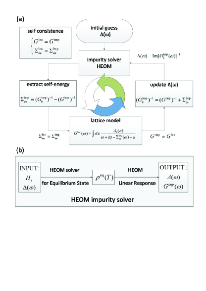
Figure 1: (Color online). (a) Flow chart of the HEOM based DMFT approach. (b) Schematic diagram of the HEOM impurity solver.

The overall framework of HEOM-based DMFT is presented in the flow chart of Fig. 1(a), while the numerical procedures involved in the HEOM impurity solver is sketched in Fig. 1(b). The HEOM impurity solver starts with the pre-determined system Hamiltonian $H_{s}$ and the input hybridization function $\Delta(\omega)$. First, the HEOM of Eq. (II.1) is solved to obtain the equilibrium-state reduced density matrix and auxiliary density matrices $\bm{\rho}^{\rm eq}(T)\equiv\big{\{}\rho^{(n);\,{\rm eq}}_{j_{1}\cdots j_{n}}(T);\,n=0,\cdots\!,L\big{\}}$. Then, the system correlation functions can be obtained by solving the HEOM-space linear problem of Eq. (28) for each frequency point. Finally, the impurity spectral function and Green’s function are evaluated through Eqs. (29) and (30), which are used to construct a new hybridization function via the lattice Green’s function.

For achieving the optimal efficiency of HEOM, a multi-Lorentzian decomposition schemeZhe10114101 ; Xie12044113 for the hybridization function $\Delta(\omega)$ is adopted. In this way, the hybridization function is spanned by a set of Lorentzian functions $\Delta(\omega)\equiv\sum_{i=1}^{N}\Delta_{i}(\omega)=\sum_{i=1}^{N}\frac{\Gamma_{i}W_{i}^{2}}{(\omega-\Omega_{i})^{2}+W_{i}^{2}}$. The parameters $\Omega_{i},\Gamma_{i}$ and $W_{i}$ for each Lorentzian function are obtained by a least square fit. As the hybridization function is updated in each DMFT iteration, the number of the Lorentzian functions $N$ is tuned case by case to find the minimal $N$ with sufficient fitting accuracy.

Figure 2: (Color online). The Lorentzian fit of the hybridization function. The number of Lorentzian functions used is $N=9$ for (a) and $N=16$ for (b).

As shown in Fig. 2, two typical hybridization functions are fitted by Lorentzian functions. For a hybridization function with a well-defined peak structure, $N=9$ is sufficient to reach a reasonable accuracy; see Fig. 2(a). However, for a hybridization function possessing a complex peak structure, a larger $N$ is necessary to reach the same level of fitting accuracy. As shown in Fig. 2(b), the presence of a small and narrow peak at the Fermi energy requires $N=16$ for an accurate fitting. At present, the major bottleneck of the HEOM approach is the physical memory required to store all the auxiliary density matrices (rather than the CPU time), with the total number of ${\cal N}(K,L)=\sum_{n=0}^{L}\frac{K!}{n!(K-n)!}$, where $K=4M$, as described earlier (see Sec. II.1) for single impurity systems, with $M$ being the number of the Lorentzian function plus the number of Padé decomposition term for the Fermi function. For a typical calculation in this work, the maximum memory required using Lorentzian number $N=9$ is about 2361 MB, while the memory required for $N=18$ is 11366 MB (see Table 1).

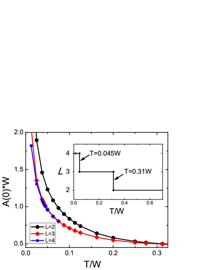
Figure 3: (Color online). Spectral function $A(\omega=0)$ as a function of temperature for truncation level $L=2\sim 4.$ The inset shows the minimal $L$ that is necessary to achieve quantitative convergence at different temperatures.

The nonperturbative feature of HEOM ensures it is applicable to SCS of a wide range of system parameters. It goes with a well-defined convergence scheme determined by the truncation level $L$, without any tricky parameters to deal with. The convergence of the dynamical quantities for quantum impurity systems is guaranteed once convergence with respect to truncation level $L$ is reached. The minimal truncation level $L$ required to achieve convergence is closely dependent on the system configuration and the surrounding environment, such as the strength of electron correlation, the system-reservoir coupling, and the temperature. It is difficult to have an a priori estimation for the required minimal $L$. In practice, the convergence of HEOM with respect to $L$ is tested case by case. In Fig. 3, we demonstrate such a convergence test for different temperatures. The spectral function $A(\omega=0)$ is monitored for various combinations of $L$ and $T$. For the lowest temperature $T=0.0125W$ involved in this work, $L=4$ is necessary (data for $L=5$ are not shown). As the temperature increases to $T=0.045W$ and $T=0.31W$, $L=3$ and $L=2$ are sufficient for convergence, respectively. In this work, all the results presented are affirmed as already converged at $L\leqslant 4$.

In fact, the HEOM solver retains its accuracy and becomes even more efficient at high temperatures. In practice, the HEOM solver is applicable to an arbitrary finite temperature, provided with sufficient computational resources. Therefore, it is possible to investigate temperature sensitive electron correlation effects by continuously varying the temperature. Furthermore, the HEOM approach works in the real frequency domain, and hence avoids invoking the numerically ill-defined analytical continuation problems for approaches working in the imaginary frequency domain.

$\qquad L$	$\qquad N$	CPU time (s)	Memory (MB)
1	9	2	0.2
2	9	34	9
3	9	959	175
4	9	48934	2361
5	9	302174	21378
4	14	99356	5584
4	18	1637256	11366

Table 1: CPU time (in unit of second) and memory (in unit of megabyte) used for typical HEOM calculations on a PC with a 3.0GHz frequency CPU. $L$ is the truncation level, and $N$ is number of the Lorentzian functions used for the decomposition of system-reservoir hybridization function.

The major limitation of the current HEOM implementation is that the computational cost increases dramatically as the system temperature decreases. This is because for a lower temperature, a larger number of memory components ($M$ in Eq. (10)) and a higher truncation level ($L$) are necessary to ensure numerical convergence, leading to a rapid growth of the total number ${\cal N}(K,L)$ of auxiliary density matrices involved in the HEOM formalism. In Table 1, we collect the CPU time and memory usage information for some typical HEOM impurity solver calculations. In practical calculations, parallel programming techniques have been employed to reduce the computational time. The lowest temperature we are able to access with the computational resources at our disposal is $T=0.0125W$, in which $W$ is the effective bandwidth of the noninteracting lattice density of states. Actually, the current HEOM implementation is mainly limited by the insufficient physical memory to store all the auxiliary density matrices (rather than CPU time), as mentioned earlier. Fortunately, it is possible to improve substantially the efficiency of HEOM by removing part of the auxiliary density matrices those are exactly zero based on physical consideration. This forthcoming improvement may realize the investigations of SCS using the HEOM based DMFT at further lower temperatures.

III results and discussions

The Mott metal-insulator transition is one of the best test beds for the accuracy and efficiency of the DMFT implementation. In this work we focus on the Mott transition in the half-filling paramagnetic phase at finite temperature. Employing our developed DMFT approach using the HEOM impurity solver, we calculate the spectral functions of SCS, and compare our results with those obtained by Bulla et al.Bul99136 ; Bul01045103 who used an NRG impurity solver along with a “patching method” for the evaluation of spectral functions.

The calculations are performed on both the hypercubic lattice with infinite dimension and the Bethe lattice with infinite coordination number. The noninteracting density of states for these two lattices are

$$A_{0}^{\rm h}(\epsilon)=\frac{1}{\tilde{t}\sqrt{2\pi}}\exp(-\frac{\epsilon^{2}}{2{\tilde{t}}^{2}}),$$ (38)

and

$$A_{0}^{\rm B}(\epsilon)=\frac{1}{2\pi{\tilde{t}}^{2}}\sqrt{4{\tilde{t}}^{2}-\epsilon^{2}};\qquad|\epsilon|\leqslant 2\tilde{t}.$$ (39)

The effective bandwidth, defined as $W\equiv 4[{\int d\epsilon A_{0}(\epsilon)\epsilon^{2}}]^{\frac{1}{2}}$, is calculated to be $W=4\tilde{t}$ for both the hypercubic and the Bethe lattices.Bul99136 In this work, $\tilde{t}$ is set to unity, and $W=4$ is set as the energy scale. To ensure the half-filling of the impurity system, a symmetric Anderson impurity model is employed, and the chemical potential is set to zero.

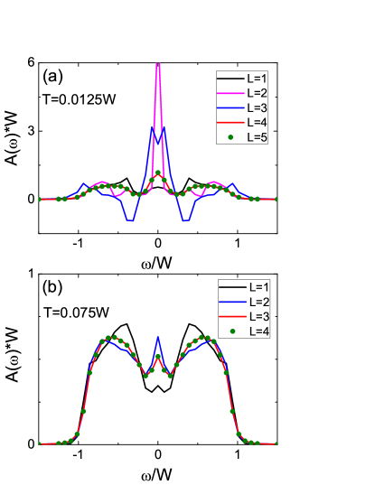
Figure 4: (Color online). The convergence of the spectral function with respect to the truncation level $L$ for Bethe lattice at (a) $T=0.0125W$ and (b) $T=0.075W$. Here, $U=W$ with $W$ being the effective bandwidth.

The convergence of the DMFT method using the HEOM impurity solver versus the truncation level $L$ is examined, and shown in Fig. 4. At the lowest temperature performed in our study, $T=0.0125W$, the calculated spectral function is converged at $L=4$. At a truncation level lower than ($L<4$), the resulted $A(\omega)$ are not accurate enough, even qualitatively. Sometimes even unphysical results may appear, such as the negative spectral function at $L=3$. The typical time for a single DMFT iteration at truncation level $L=4$ is about 6 hours on a PC with a 3.0GHz frequency CPU. When the temperature increases to $T=0.075W$, $L=3$ is sufficient for the convergence of the resulting spectral function. At this truncation level, the typical time for a single DMFT iteration dramatically decreases to less than 30 minutes. In this work, the convergence of all the data represented has been carefully checked.

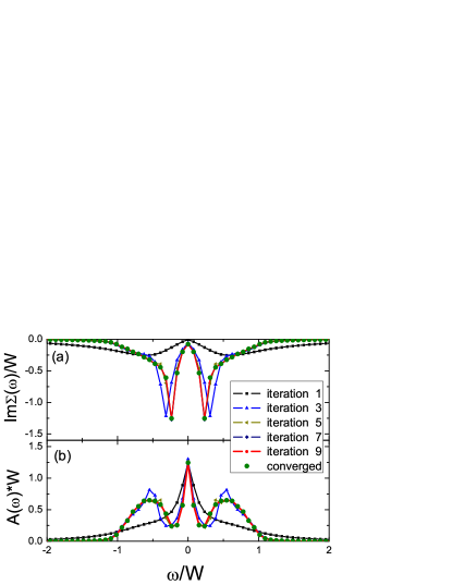
Figure 5: (Color online). The convergence of (a) the self-energy and (b) the spectral function for a hypercubic lattice by iteration. The parameters are $U=W$ and $T=0.0125W$, where $W$ is the effective bandwidth.

The DMFT iteration, calculated by using the proposed method, is usually converged within 10 iterations for systems away from the metal-insulator transition region. As an example, we show in Fig. 5 the convergence of the spectral function and self-energy in hypercubic lattice by iteration, with the parameter $U=W$ and $T=0.0125W$. The initial hybridization function can be obtained by setting the initial electron-electron self-energy to zero. Alternatively, in this work we choose to use the initial hybridization in the form of a single Lorentzian function centered at the Fermi level. We have confirmed that they converge to the same final self-energy and spectral function. By adopting the single Lorentzian type initial hybridization function, numerical convergence is reached within 10 DMFT iterations. However, more iterations are necessary to achieve convergence when the system is near to the phase transition area.

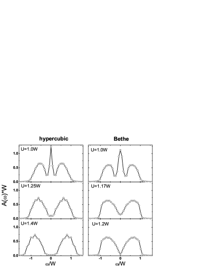
Figure 6: Spectral functions of the hypercubic lattice and the Bethe lattice with different values of $U$. The temperature is $T=0.0125W$, where $W$ is the effective bandwidth.

We report in Fig. 6 the spectral functions $A(\omega)$, with different values of $U$ at finite temperature $T=0.0125W$, for both the hypercubic lattice and the Bethe lattice. These two lattices have similar behaviors. For $U=W$ both show metallic three-peak characteristics, with a quasi-particle peak at the Fermi level. Further increasing the values of $U$, the height of quasi-particle peak decreases abruptly to a nearly zero value at a critical $U_{c}$ (see the $T=0.0125W$ line in the inset of Fig. 9), leading to a transition from metal to insulator. The transition behavior is very similar to the zero temperature spectral function,Bul99136 except for that the quasi-particle peaks are slightly broadened and lowered at finite temperature.

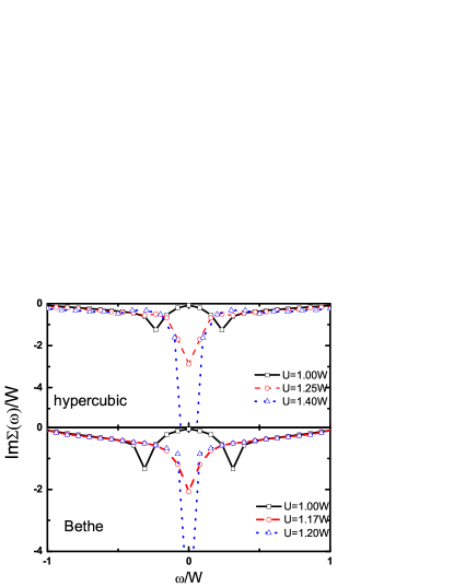
Figure 7: (Color online). The imaginary part of the self-energy of hypercubic (upper panel) and Bethe (lower panel) lattices at different values of $U$. The temperature is $T=0.0125W$, where $W$ is the effective bandwidth.

The corresponding converged self-energies are shown in Fig. 7 for both the hypercubic and the Bethe lattice systems at the same temperature. For $U=W$, the two-peak structure of the imaginary part of the self-energy gives rise to the three-peak structure in the spectral function. This is because the peaks in the imaginary part of the self-energy induce dips in the spectral function. With the increase of the value of $U$, the peaks in the imaginary self-energy around the Fermi energy show up, leading to the vanishing of the quasi-particle peaks in the spectral function. The peaks around the Fermi energy in the imaginary self-energy are also broadened by the finite temperature. Thus the critical value of $U$ for metal-insulator transition would not depend on temperature.Bul01045103

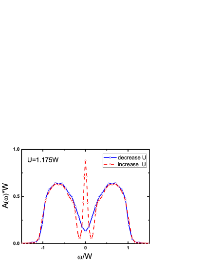
Figure 8: (Color online). Existence of dual solution for the spectral function at $T=0.0125W$ and $U=1.175W$. The two solutions are obtained by increasing and decreasing the value of $U$ gradually to $1.175W$, respectively.

For the numerical aspect, the computational cost (time and memory) of present HEOM approach grows rapidly with the lowered $T$ as higher truncation level is needed for convergence. Currently the lowest temperature that is available for the present HEOM algorithm as DMFT impurity solver is $T=0.0125W$.

As will be shown in the following part of this section, this currently HEOM achievable temperature is already lower than the critical temperature $T_{\rm c}\approx 0.02W$ for first-order Mott-Hubbard metal-insulator transition of the Bethe lattice.Bul01045103 One of the main feature for $T<T_{\rm c}$ is the coexistence of both the metallic and insulating solutions within a certain range of $U$.Bul01045103 ; Fel04136405 This phenomenon is also found in our calculation, as shown in Fig. 8. When $U=1.175W$ at $T=0.0125W$, a metallic three-peak spectral function is obtained if the initial spectral function is also metallic. In this case, the converged spectral function of a lattice system with a smaller $U$ is used as the initial guess. Whereas if a converged insulating spectral function corresponding to a lattice system with a larger $U$ is feeded as the initial guess, the resulted spectral function has a dramatically depressed component around the Fermi energy. It is noted that for the “insulating” solution in Fig. 8, the spectral function around the Fermi energy is nonzero although the value is very small. This is possibly because that the finite temperature of $T=0.0125W$ is very close to $T_{\rm c}$.

One of the advantages of the HEOM approach is that it is even more convenient to achieve quantitative accuracy at higher temperatures. This feature ensures the continuous variation of the temperature to investigate possible temperature sensitive phase transitions. It should be noted that when the temperature increases, the efficiency of the HEOM approach is dramatically enhanced. For example, the calculation speed for single DMFT iteration at $T=0.075W$ is more than ten times faster than that at $T=0.0125W$. Figure 9 depicts the spectral functions $A(\omega)$ and both the real and imaginary parts of the self-energies of Bethe lattice. The value of $U$ is fixed to $U=W$, while the temperature is varied from $T=0.0125W$ to $T=0.1W$. At $T=0.0125W$, the spectral function has the typical three-peak feature. When the temperature increases, the quasi-particle peak shrinks continuously. This change is also reflected in the corresponding self-energy. For example, by increasing the temperature, the two peaks in the imaginary part of the self-energy at low temperature become smaller and move toward the Fermi energy. Finally, these peaks disappear at high temperature $T=0.1W$, and a peak around the Fermi energy shows up.

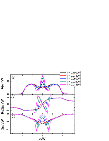
Figure 9: (Color online). (a) Spectral function $A(\omega)$, (b) real part of self-energy, and (c) imaginary part of self-energy at different temperatures for a Bethe lattice. Here, $U=W$ with $W$ being the effective bandwidth.

Although the quasi-particle peak shrinks in the spectral function as shown in Fig. 9, the system of $U=W$ remains in the metallic state. However, by tuning the values of $U$, metal-insulator transition may occur as the temperature varies.

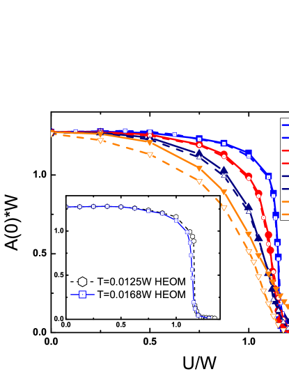
Figure 10: (Color online). Comparison of $A(\omega=0)$ vs $U$ between DMFT methods using HEOM and NRG impurity solvers. Various temperatures are examined. The inset shows the HEOM obtained $A(\omega=0)$ versus $U$ for temperature $T=0.0168W$ and $T=0.0125W$. The NRG data are extracted from Ref. Bul01045103, .

In the following, we focus on the $U$ dependence of the spectral function at the Fermi energy $A(\omega=0)$ at different temperatures, and compare to the results obtained by the NRG method.Bul01045103 The comparison is shown in Fig. 10. At some low temperatures, for instance, $T=0.0168W$ or $T=0.0276W$, the HEOM results agree quantitatively with those obtained by the NRG method. As $U$ increases from zero, $A(\omega=0)$ decreases to zero at a certain value of $U$. Such a value depends on the temperature. Moreover, as shown in the inset, while the HEOM calculated $A(\omega=0)$ gradually decreases to zero at $T=0.0168W$, at $T=0.0125W$ the curve exhibits an abrupt decrease around $U=1.17W$. This indicates a first-order phase transition at $T=0.0125W$.

As the temperature increases further, the HEOM results start to deviate from the NRG data; see Fig. 10. The deviation is one-sided, meaning that the HEOM calculated $A(\omega=0)$ is always smaller than that obtained by the NRG method, and the magnitude of deviation increases consistently versus temperature.

It has been elaborated in the Sec. II that the HEOM approach is in principle numerically exact. Meanwhile, the NRG method is also considered as a numerically exact impurity solver. Therefore, it is intriguing why the two in-principle exact approaches would give different results at the somewhat high temperature $T=0.0741W$. To clarify this issue, we emphasize here that the numerical exactness of a certain approach is achieved only when the computation results converge quantitatively with respect to all the involving parameters.

To understand the discrepancy between the HEOM and NRG results obtained at the high temperature, we now check the numerical convergence of both impurity solvers, for the same system and with the same hybridization function.

For the HEOM approach, there are only two controlling parameters, the memory component $M$ in Eq. (10) and the truncation level $L$. Its convergence with respect to these two parameters have already been affirmed; see Figs. 2, 3 and 4. It can be seen that the convergence of the HEOM approach is much easier at high temperature than that at low temperature, as by construction it is intrinsically more favorable at higher temperature cases. The convergence of all the HEOM results shown in Fig. 10 and Fig. 11 have also been carefully checked.

In contrast, the NRG approach used in Ref. Bul01045103, involves several controlling parameters. The most important two are the discretization parameter $\Lambda$ and the number of kept states $M_{s}$. The NRG results are considered to be numerically exact if they converge as $\Lambda\rightarrow 1$ and $M_{s}\rightarrow\infty$. However, it is usually very difficult to reach at high temperature, due to the exponential increase of the computational cost. The NRG dataBul01045103 we cited in Fig. 10 were obtained under $\Lambda=1.64$, and the convergence was not reported. Therefore, we carry out a check of its convergence for both low and high temperatures; see Fig. 11.

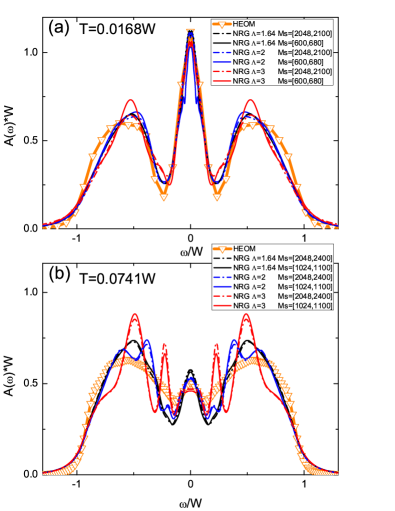
Figure 11: (Color online). Spectral functions obtained by the NRG approach used in Ref. Bul01045103, with different values of the controlling parameters $\Lambda$ and $M_{s}$, at $T=$ (a) $0.0168W$ and (b) $0.0741W$. The expression $M_{s}=[a,b]$ with numbers $b>a$ means that the actual value of $M_{s}$ is chosen in the interval $[a,b]$ with the largest energy gap. The hybridization functions are extracted from the HEOM converged results, and are used for both impurity solvers. The corresponding HEOM calculated spectral functions are also shown for comparison.

Figure 11 shows that the NRG results converge rapidly with respect to $\Lambda$ and $M_{s}$ at low temperature, but rather slowly at high temperature, which is very different (or opposite to) the HEOM approach. At the low temperature $T=0.0168W$, the overall shape of the best NRG curve with $\Lambda=1.64$ and $M_{s}=[2048,2100]$ is very close to the HEOM converged spectral function, which is consistent with the fact that at low temperature the data in Fig. 10 are almost identical. Here $M_{s}=[2048,2100]$ means that the actual value of $M_{s}$ is chosen between 2048 and 2100 with the largest energy gap. At high temperature $T=0.0741W$, the best NRG spectral function with $\Lambda=1.64$ and $M_{s}=[2048,2400]$ in our calculation is still not guaranteed to be converged. Moreover, its overall shape dramatically differs from the converged HEOM one. It indicates that large uncertainties reside in the $T=0.0741W$ NRG data shown in Fig. 10.

It should be pointed out that the NRG data of Ref. Bul01045103, used for the comparison in Fig. 10 do not represent the best possible NRG results. In the past decade, the quality of the spectral function produced by NRG has been improved dramatically by the new algorithms such as the density matrix NRGHof001508 and the full density matrix NRG.Wei07076402 ; Pet06245114 We have also checked the convergence of the corresponding spectral function at $T=0.0741W$ using the full density matrix NRG approach; see Supplemental Material.Sup The resulted spectral function is overall much closer to the HEOM counterpart, including the heights of the Kondo and the Hubbard peaks, and the overall line shape of the dip between them.Sup

At this stage, the origin of the remaining difference between the HEOM and NRG spectral functions displayed in Fig. 11(a) is unclear. Clarifying this issue requires a more careful and comprehensive assessment of the NRG methods (since the HEOM data have converged). However, this could be technically very difficult, and is beyond the scope of this paper. Therefore, this problem is left open for further investigations.

IV Concluding Remarks

To summarize, the HEOM approach is used as the impurity solver for DMFT method. This method is employed to investigate the Mott-Hubbard metal-insulator transition in both the hypercubic and the Bethe lattices at finite temperature. At low temperatures the results obtained by the HEOM based DMFT method agree well with those using the NRG method as the impurity solver. At higher temperatures, the HEOM approach becomes much more efficient. Thus the HEOM approach provides a complement to the NRG impurity solver, in the sense that it is highly efficient and converges rapidly at finite temperatures.

Currently the developed approach is limited to a temperature no lower than $T=0.0125W$. The reason is that at lower temperature the numeric convergence requires larger truncation level. It is however possible to design more efficient reservoir memory decomposition schemes to dramatically reduce the computational resources requirements. The Lorentzian fit scheme for evaluating the hybridization function may also introduce minor residual error under certain circumstances. For example, the quasi-particle peak at the Fermi level becomes quite narrow when the system is very near to the metal-insulator transition point. To distinguish this type of peak in the process of Lorentzian fit, much finer frequency meshes near the Fermi level is necessary. It will sometimes lead to minor fitting error for the narrow quasi-particle peak.

The HEOM approach adopts a general form of the system Hamiltonian. It is quite convenient to extend the current HEOM+DMFT approach to systems other than the half-filled single-band situation. For example, the system occupation number can be tuned away from half-filling by the adjustment of the chemical potential, to simulate the influence of charge doping to SCS. In this situation, the asymmetric Anderson impurity model is to be employed in the HEOM impurity solver, and an additional search is required for the correct chemical potential that reproduces the true occupation number on a lattice site.

The HEOM approach is also applicable to complicated multi-orbital impurity models. For instance, the HEOM approach has been applied to a three-impurity Anderson model; see Fig. S8 in the Supplemental Material of Ref. Li12266403, . This confirms the potential applicability of the HEOM method to more complex systems. Moreover, it is possible to improve further the efficiency of HEOM approach based on physical considerations and making use of the sparse nature of HEOM. This may extend further the applicability of HEOM+DMFT method to further complex strongly correlated systems.

- (1) P. Fulde, Electron Correlations in Molecules and Solids, Springer-Verlag, Berlin Heidelberg, 1991.
- (2) W. Metzner and D. Vollhardt, Phys. Rev. Lett. 62, 324 (1989).
- (3) M. Jarrell, Phys. Rev. Lett. 69, 168 (1992).
- (4) A. Georges and G. Kotliar, Phys. Rev. B 45, 6479 (1992).
- (5) A. Georges, G. Kotliar, W. Krauth, and M. J. Rozenberg, Rev. Mod. Phys. 68, 13 (1996).
- (6) X. Y. Zhang, M. J. Rozenberg, and G. Kotliar, Phys. Rev. Lett. 70, 1666 (1993).
- (7) F. Gebhard, The Mott Metal-Insulator Transition: Models and Methods. (Springer Tracts in Modern Physics), Springer-Verlag, Berlin Heidelberg, 1997.
- (8) M. Imada, A. Fujimori, and Y. Tokura, Rev. Mod. Phys. 70, 1039 (1998).
- (9) A. Georges and W. Krauth, Phys. Rev. B 48, 7167 (1993).
- (10) M. J. Rozenberg, G. Kotliar, and X. Y. Zhang, Phys. Rev. B 49, 10181 (1994).
- (11) M. J. Rozenberg, R. Chitra, and G. Kotliar, Phys. Rev. Lett. 83, 3498 (1999).
- (12) R. Bulla, Phys. Rev. Lett. 83, 136 (1999).
- (13) R. Bulla, T. A. Costi, and D. Vollhardt, Phys. Rev. B 64, 045103 (2001).
- (14) X. Dai, K. Haule, and G. Kotliar, Phys. Rev. B 72, 045111 (2005).
- (15) Y. Ōno, M. Potthoff, and R. Bulla, Phys. Rev. B 67, 035119 (2003).
- (16) S. Florens and A. Georges, Phys. Rev. B 66, 165111.
- (17) Q. Si and J. L. Smith, Phys. Rev. Lett. 77, 3391 (1996).
- (18) R. Chitra and G. Kotliar, Phys. Rev. Lett. 84, 3678 (2000).
- (19) G. Kotliar and S. Savrasov, in New Theoretical Approaches to Strongly Correlated Systems, edited by A. M. Tsvelik, pages 259–301, Kluwer Academic, Dordrecht, 2001.
- (20) V. Drchal, V. Jani, J. Kudrnovsk, V. S. Oudovenko, X. Dai, K. Haule, and G. Kotliar, J. Phys.: Condens. Matter 17, 61 (2005).
- (21) H. Kusunose, Journal of the Physical Society of Japan 75, 054713 (2006).
- (22) A. Toschi, A. A. Katanin, and K. Held, Phys. Rev. B 75, 045118 (2007).
- (23) V. Anisimov, A. Poteryaev, M. Korotin, A. Anokhin, and G. Kotliar, Journal of Physics: Condensed Matter 9, 7359 (1997).
- (24) G. Kotliar, S. Y. Savrasov, K. Haule, V. S. Oudovenko, O. Parcollet, and C. A. Marianetti, Rev. Mod. Phys. 78, 865 (2006).
- (25) H. Kajueter, G. Kotliar, and G. Moeller, Phys. Rev. B 53, 16214 (1996).
- (26) N. E. Bickers, Rev. Mod. Phys. 59, 845 (1987).
- (27) E. Dagotto, Rev. Mod. Phys. 66, 763 (1994).
- (28) M. Caffarel and W. Krauth, Phys. Rev. Lett. 72, 1545 (1994).
- (29) Q. Si, M. J. Rozenberg, G. Kotliar, and A. E. Ruckenstein, Phys. Rev. Lett. 72, 2761 (1994).
- (30) J. E. Hirsch and R. M. Fye, Phys. Rev. Lett. 56, 2521 (1986).
- (31) E. Gull, A. J. Millis, A. I. Lichtenstein, A. N. Rubtsov, M. Troyer, and P. Werner, Rev. Mod. Phys. 83, 349 (2011).
- (32) K. G. Wilson, Rev. Mod. Phys. 47, 773 (1975).
- (33) R. Bulla, T. A. Costi, and T. Pruschke, Rev. Mod. Phys. 80, 395 (2008).
- (34) W. Hofstetter, Phys. Rev. Lett. 85, 1508 (2000).
- (35) A. Weichselbaum and J. von Delft, Phys. Rev. Lett. 99, 076402 (2007).
- (36) R. Peters, T. Pruschke, and F. B. Anders, Phys. Rev. B 74, 245114 (2006).
- (37) P. W. Anderson, Phys. Rev. 124, 41 (1961).
- (38) J. Hubbard, Proc. Roy. Soc. A 276, 238 (1963).
- (39) P. A. Lee, T. M. Rice, J. W. Serene, L. J. Sham, and J. W. Wilkins, Comments on Cond. Matter Phys. 12, 99 (1986).
- (40) V. Anisimov and Y. Izyumov, Electronic Structure of Strongly Correlated Materials, Springer-Verlag, Berlin Heidelberg, 2010.
- (41) Z. H. Li, N. H. Tong, X. Zheng, D. Hou, J. H. Wei, J. Hu, and Y. J. Yan, Phys. Rev. Lett. 109, 266403 (2012).
- (42) M. Jarrell and J. Gubernatis, Phys. Rep. 269, 133 (1996).
- (43) J. S. Jin, X. Zheng, and Y. J. Yan, J. Chem. Phys. 128, 234703 (2008).
- (44) R. P. Feynman and F. L. Vernon, Jr., Ann. Phys. 24, 118 (1963).
- (45) H. Kleinert, Path Integrals in Quantum Mechanics, Statistics, Polymer Physics, and Financial Markets, World Scientific, Singapore, 2009, 5th ed.
- (46) R. X. Xu, P. Cui, X. Q. Li, Y. Mo, and Y. J. Yan, J. Chem. Phys. 122, 041103 (2005).
- (47) R. X. Xu and Y. J. Yan, Phys. Rev. E 75, 031107 (2007).
- (48) X. Zheng, J. S. Jin, and Y. J. Yan, J. Chem. Phys. 129, 184112 (2008).
- (49) S. K. Wang, X. Zheng, J. S. Jin, and Y. J. Yan, Phys. Rev. B 88, 035129 (2013).
- (50) X. Zheng, J. S. Jin, and Y. J. Yan, New J. Phys. 10, 093016 (2008).
- (51) X. Zheng, J. S. Jin, S. Welack, M. Luo, and Y. J. Yan, J. Chem. Phys. 130, 164708 (2009).
- (52) X. Zheng, Y. J. Yan, and M. Di Ventra, Phys. Rev. Lett. 111, 086601 (2013).
- (53) X. Zheng, R. X. Xu, J. Xu, J. S. Jin, J. Hu, and Y. J. Yan, Prog. Chem. 24, 1129 (2012).
- (54) A. Croy and U. Saalmann, Phys. Rev. B 80, 073102 (2009).
- (55) T. Ozaki, Phys. Rev. B 75, 035123 (2007).
- (56) J. Hu, R. X. Xu, and Y. J. Yan, J. Chem. Phys. 133, 101106 (2010).
- (57) J. Hu, M. Luo, F. Jiang, R. X. Xu, and Y. J. Yan, J. Chem. Phys. 134, 244106 (2011).
- (58) R. Wang, D. Hou, and X. Zheng, Physical Review B 88, 205126 (2013).
- (59) R. W. Freund and N. M. Nachtigal, SIAM J. Numer. Math. 60, 315 (1991).
- (60) R. W. Freund, SIAM J. Sci. Comput. 14, 470 (1993).
- (61) X. Zheng, G. Chen, Y. Mo, S. K. Koo, H. Tian, C. Y. Yam, and Y. J. Yan, J. Chem. Phys. 133, 114101 (2010).
- (62) H. Xie, F. Jiang, H. Tian, X. Zheng, Y. Kwok, S. Chen, C. Y. Yam, Y. J. Yan, and G. Chen, J. Chem. Phys. 137, 044113 (2012).
- (63) M. Feldbacher, K. Held, and F. F. Assaad, Phys. Rev. Lett. 93, 136405 (2004).
- (64) See Supplemental Material xxx for a comparison between the HEOM and full density matrix NRG impurity solvers.